跳到论文正文
W Papers独立论文阅读器 arXiv:1412.3395 论文正文 计算阅读时间 · 0%
引用这篇论文根据当前论文元数据生成,正式投稿前建议核对。


License: arXiv.org perpetual non-exclusive license
arXiv:1412.3395v2 [hep-th] 29 Aug 2016

DESY 14-236
HU-Mathematik-35-2014
HU-EP-14/57

Toda 3-Point

Functions
From Topological Strings II

Mikhail Isachenkova, Vladimir Mitevb, Elli Pomonia,c

aDESY Hamburg, Theory Group,
Notkestrasse 85, D–22607 Hamburg, Germany

bInstitut für Mathematik und Institut für Physik,
Humboldt-Universität zu Berlin
IRIS Haus, Zum Großen Windkanal 6, 12489 Berlin, Germany

cPhysics Division, National Technical University of Athens,
15780 Zografou Campus, Athens, Greece

mikhail.isachenkov@desy.de
mitev@math.hu-berlin.de
elli.pomoni@desy.de

Abstract

In [1] we proposed a formula for the 3-point structure constants of generic primary fields in the Toda field theory, derived using topological strings and the AGT-W correspondence from the partition functions of the non-Lagrangian TNT_{N} theories on S4S^{4}. In this article, we obtain from it the well-known formula by Fateev and Litvinov and show that the degeneration on a first level of one of the three primary fields on the Toda side corresponds to a particular Higgsing of the TNT_{N} theories.

1 Introduction

Two-dimensional conformal field theories (CFTs) include many models with important physical applications and have provided a rich playground for exact solutions of CFTs. Even though extensive methods have been developed for rational CFTs throughout the years [2], non-rational 2D CFTs are much less understood. So far, all non-rational CFTs that have been solved are versions of Liouville. A CFT is solved when its two and three point correlation functions are obtained and a crucial step in doing this for the Liouville CFT was the proposal of the 3-point function by Dorn-Otto-Zamolodchikov-Zamolodchikov (DOZZ) [3, 4] based on insightful and powerful consistency checks. This proposal was rigorously derived by Teschner [5] who showed that the DOZZ 3-point function is a solution of the crossing symmetry equation.

The next natural step is to study multifield non-rational CFTs, a prototype of which is the Toda CFT. Obtaining the 3-point functions of the Toda CFT is a long-standing problem in mathematical physics. Attacking this problem purely by using 2D CFT techniques is a notoriously difficult task and results exist only for particular specializations of the external momenta. The state of the art can be found in the works of Fateev and Litvinov [6, 7, 8], who obtained the 3-point functions of primary operators if one of them is appropriately degenerate.

In a previous publication [1], we presented a formula for the 3-point functions of three arbitrary primaries of the Toda CFT. Our formula (16) was obtained using techniques of a very different nature than [6, 7, 8], namely topological stings, 5-brane web physics and the AGT-W correspondence. The purpose of the present paper is to push forward the program of further understanding and checking it. We begin with (16), specialize appropriately one of the external momenta and obtain the formula of Fateev-Litvinov [6] after a direct calculation, thus presenting a highly non-trivial check of our proposal. Specializing means that the Verma module for the primary field has a null-vector descendant at level one. In the rest of the paper, we will refer to them as semi-degenerate11 1 A representation of WN can contain a null vector at some level higher than one. Such representations are called semi-degenerate as well. The 3-point functions containing one primary belonging to such representation and two generic ones will not be considered in the present paper., as opposed to the completely degenerate ones, containing N−1N-1 linearly independent null-vectors. Furthermore, we believe that the techniques of [1] will provide the solution not only for the 3-points functions of WN\textbf{W}_{N} primaries, but also for those involving descendent fields. We leave this for a future work.

The quirks of our formula for the 3-point functions (16) stem from the strategy employed in [1] to derive it. A key element was the AGT-W correspondence [9, 10], which is a relation between 4D 𝒩=2\mathcal{N}=2 SU​(N)\text{SU}(N) quiver gauge theories and the 2D WN\textbf{W}_{N} Toda CFT. Specifically, upon an appropriate identification of the parameters, the correlation functions of the 2D Toda CFT are equal to the partition functions of the corresponding 4D 𝒩=2\mathcal{N}=2 gauge theories. The conformal blocks of the 2D CFTs are given by the instanton partition functions of Nekrasov [9, 10], while the 3-point structure constants are obtained by the partition functions of the TNT_{N} superconformal theories [11, 12]. The TNT_{N} theories have no Lagrangian description and thus their partition functions were unknown until recently [1, 12, 13]. The sole exception was the W2≡𝐕𝐢𝐫{}_{2}\equiv\bf{Vir} case, i.e. the Liouville case, whose 3-point structure constants are given by the famous DOZZ formula [3, 4] and equal to the partition function of four free hypermultiplets [14, 12].

We were able to bypass the fact that the TNT_{N} theories have no known Lagrangian description by using a generalized version of AGT-W: a relation between 5D gauge theories compactified on S1S^{1} and 2D qq-deformed Liouville/Toda CFT [15, 16, 17, 18, 19, 20, 21, 12, 22, 23, 24, 25, 26, 27, 28], where the circumference β\beta of the S1S^{1} corresponds to the deformation parameter q=e−βq=e^{-\beta} of the CFT. In 5D, the partition functions can be computed not only using localization, which requires a Lagrangian, but also by using the powerful tool of topological strings [29]. Employing this technology, we calculated in [12] (see also [13]) the partition functions of the 5D TNT_{N} theories and suggested that they should be interpreted as the 3-point structure constants of the qq-deformed Toda. Subsequently, we showed in [1] how to take the 4D limit, corresponding to β→0\beta\rightarrow 0 or equivalently to q→1q\rightarrow 1, thus obtaining the partition function (21) of the 4D TNT_{N} theories. We want to stress that taking this limit is a tricky business, as the expression (16) includes non-trivial multiple sums and integrals. This is the reason why we will always work with the qq-deformed formulas and take the limit only at the end.

This article is organized as follows. After briefly reminding the reader of the essentials of Toda CFTs, we recall the formula by Fateev and Litvinov for a special class of 3-point functions of Toda primaries, as well as its straightforward generalization to the conjectural qq-deformed Toda theory. We then conclude section 2 by quoting our general proposal for generic 3-point functions of Toda primaries. To spell out the details of it, we will need some basics of the AGT dictionary collected in section 3. In the next section 4, the discussion temporarily deviates from the CFT matters focusing rather on the interplay between the moduli spaces of the corresponding gauge theories and 5-brane web physics. We argue that the semi-degeneration of a primary field on the (qq-deformed) CFT side mirrors a Higgsing of the TNT_{N} theory on the 4D (5D) side. A more CFT-oriented reader can skip this section, with the exception of 4.3. The AGT genesis of Fateev-Litvinov formula for W3 Toda 3-point function, via pinching an integration contour by a particular residue of the corresponding integrand and applying non-trivial summation theorems, is what section 5 focuses upon. With the details of W4 computation deferred to the appendix C, we then proceed to a discussion of the general WN case in section 6. The conclusion and the outlook follow, whereas the remaining appendices are devoted to overview of notations and special functions, most importantly to describing and elaborating on the properties of the Kaneko-Macdonald-Warnaar sl​(N)\text{sl}(N) hypergeometric functions which play a major role in our calculations.

2 Toda CFT: a recap and a proposal

In this section we briefly summarize some relevant facts about the Toda CFT, closely following [6, 7, 8]. Furthermore, we spell out the Fateev-Litvinov formula for a special subset of Toda structure constants and present our proposal for the Toda 3-point functions of generic primary fields.

The Lagrangian of the AN−1A_{N-1} Toda CFT is given by

L=18​π​(∂νφ,∂νφ)+μ​∑k=1N−1eb⁡(ek,φ),L=\frac{1}{8\pi}\left(\partial_{\nu}\varphi,\partial^{\nu}\varphi\right)+\mu\sum_{k=1}^{N-1}e^{b\left(e_{k},\varphi\right)}, (1)

where φ:⁣=∑i=1N−1φiωi\varphi\mathrel{\mathchoice{\vbox{\hbox{$\displaystyle:$}}}{\vbox{\hbox{$\textstyle:$}}}{\vbox{\hbox{$\scriptstyle:$}}}{\vbox{\hbox{$\scriptscriptstyle:$}}}{=}}\sum_{i=1}^{N-1}\varphi_{i}\omega_{i}, with eke_{k}, ωk\omega_{k} being the simple roots and the fundamental weights of sl(N)(N) respectively. The definition of the inner product (⋅,⋅)\left(\cdot,\cdot\right) along with other useful Lie-algebraic definitions and notations are collected in appendix A.2 for the convenience of the reader. The parameter μ\mu is called the cosmological constant, in analogy to the Liouville case (N=2N=2) where it determines the constant curvature of a surface described by the classical equation of motion. The normalization of the Lagrangian is chosen in such a way that

φi​(z,z¯)​φj​(0,0)=−δi​j​log​|z|2+⋯\displaystyle\varphi_{i}(z,\bar{z})\,\varphi_{j}(0,0)=-\delta_{ij}\,\text{log}|z|^{2}+\cdots  at ​z→0.\displaystyle\hskip 11.38109pt\text{ at }z\rightarrow 0. (2)

Following [7, 8], we consider the correlators on a two-sphere, which prescribes putting a background charge at the north pole in order to render the Toda action finite:

φ⁡(z,z¯)=−𝒬​log​|z|+⋯\displaystyle\varphi(z,\bar{z})=-\mathbf{\mathcal{Q}}\,\text{log}|z|+\cdots  at ​z→∞,\displaystyle\hskip 11.38109pt\text{ at }z\rightarrow\infty, (3)

where 𝒬:⁣=Qρ=(b+b−1)ρ\mathbf{\mathcal{Q}}\mathrel{\mathchoice{\vbox{\hbox{$\displaystyle:$}}}{\vbox{\hbox{$\textstyle:$}}}{\vbox{\hbox{$\scriptstyle:$}}}{\vbox{\hbox{$\scriptscriptstyle:$}}}{=}}Q\rho=(b+b^{-1})\rho with the Weyl vector ρ\rho defined in (A.8).

Analyzing the path integral of the theory (1), one can argue that the Toda CFT must have an exchange symmetry b↔b−1b\leftrightarrow b^{-1} on a quantum level which simultaneously sends the cosmological constant to its dual μ~\tilde{\mu}, defined as

(π​μ~​γ​(b−2))b=!(π​μ​γ​(b2))1b⟹μ~=(π​μ​γ​(b2))1/b2π​γ​(1/b2),\left(\pi\tilde{\mu}\gamma(b^{-2})\right)^{b}\stackrel{{\scriptstyle!}}{{=}}\left(\pi\mu\gamma(b^{2})\right)^{\frac{1}{b}}\Longrightarrow\tilde{\mu}=\frac{\left(\pi\mu\gamma(b^{2})\right)^{\nicefrac{{1}}{{b^{2}}}}}{\pi\gamma(\nicefrac{{1}}{{b^{2}}})}, (4)

where γ(x):⁣=Γ⁡(x)Γ⁡(1−x)\gamma(x)\mathrel{\mathchoice{\vbox{\hbox{$\displaystyle:$}}}{\vbox{\hbox{$\textstyle:$}}}{\vbox{\hbox{$\scriptstyle:$}}}{\vbox{\hbox{$\scriptscriptstyle:$}}}{=}}\frac{\Gamma(x)}{\Gamma(1-x)}. As we mentioned in the introduction, the Toda CFT also has a WN higher spin chiral symmetry generated by the fields W2≡TW_{2}\equiv T, W3,…,WNW_{3},\ldots,W_{N} of spins 2,…,N2,\dots,N. The primaries under the full symmetry algebra WN×W¯N\textbf{W}_{N}\times\overline{\textbf{W}}_{N} are the exponential fields of spin zero labeled by a weight of sl(N)(N):

V𝜶:⁣=e(𝜶,φ).V_{\boldsymbol{\alpha}}\mathrel{\mathchoice{\vbox{\hbox{$\displaystyle:$}}}{\vbox{\hbox{$\textstyle:$}}}{\vbox{\hbox{$\scriptstyle:$}}}{\vbox{\hbox{$\scriptscriptstyle:$}}}{=}}e^{\left(\boldsymbol{\alpha},\varphi\right)}. (5)

In what follows, we will parametrize the fundamental weight decomposition of a weight 𝜶i\boldsymbol{\alpha}_{i} as

𝜶i=N​∑j=1N−1αij​ωj.\boldsymbol{\alpha}_{i}=N\sum_{j=1}^{N-1}\alpha_{i}^{j}\omega_{j}. (6)

By looking at the corresponding OPEs, one reads off the central charge cc of the Toda CFT and the conformal dimensions Δ⁡(α)\Delta(\alpha) of its primary fields:

c=N−1+12​(𝒬,𝒬)=(N−1)​(1+N⁡(N+1)​Q2),Δ⁡(α)=(2​𝒬−𝜶,𝜶)2,c=N-1+12\left(\mathbf{\mathcal{Q}},\mathbf{\mathcal{Q}}\right)=(N-1)\left(1+N(N+1)Q^{2}\right),\qquad\Delta(\alpha)=\frac{\left(2\mathbf{\mathcal{Q}}-\boldsymbol{\alpha},\boldsymbol{\alpha}\right)}{2}, (7)

with the anti-holomorphic conformal dimensions of the primary fields being equal to the holomorphic ones.

The conformal dimension, as well as the eigenvalues of all the other higher spin currents WkW_{k} are invariant under the affine22 2 One should not confuse the affine Weyl transformation, i.e. Weyl reflections accompanied by two translations, with Weyl reflections belonging to the Weyl group of the affine Lie algebra. Weyl transformations (A.13) of the weights 𝜶i\boldsymbol{\alpha}_{i}, which roughly means that several exponential fields correspond to the same ’physical’ field. The primary fields of Toda CFT transform under an affine Weyl transformations 𝜶→𝗐∘𝜶\boldsymbol{\alpha}\rightarrow\mathsf{w}\circ\boldsymbol{\alpha} given in (A.13) as

V𝗐∘𝜶=𝖱𝗐​(𝜶)​V𝜶V_{\mathsf{w}\circ\boldsymbol{\alpha}}=\mathsf{R}^{\mathsf{w}}(\boldsymbol{\alpha})V_{\boldsymbol{\alpha}} (8)

with the reflection amplitude 𝖱\mathsf{R} given by the expression

𝖱𝗐(𝜶):⁣=𝖠⁡(𝜶)𝖠⁡(𝗐∘𝜶)\mathsf{R}^{\mathsf{w}}(\boldsymbol{\alpha})\mathrel{\mathchoice{\vbox{\hbox{$\displaystyle:$}}}{\vbox{\hbox{$\textstyle:$}}}{\vbox{\hbox{$\scriptstyle:$}}}{\vbox{\hbox{$\scriptscriptstyle:$}}}{=}}\frac{\mathsf{A}(\boldsymbol{\alpha})}{\mathsf{A}(\mathsf{w}\circ\boldsymbol{\alpha})}\, (9)

in terms of the function

𝖠(𝜶):⁣=(πμγ(b2))(𝜶−𝒬,ρ)b∏e>0Γ(1−b(𝜶−𝒬,e))Γ(−b−1(𝜶−𝒬,e)).\mathsf{A}(\boldsymbol{\alpha})\mathrel{\mathchoice{\vbox{\hbox{$\displaystyle:$}}}{\vbox{\hbox{$\textstyle:$}}}{\vbox{\hbox{$\scriptstyle:$}}}{\vbox{\hbox{$\scriptscriptstyle:$}}}{=}}\left(\pi\mu\gamma(b^{2})\right)^{\frac{\left(\boldsymbol{\alpha}-\mathbf{\mathcal{Q}},\rho\right)}{b}}\prod_{e>0}\Gamma\left(1-b\left(\boldsymbol{\alpha}-\mathbf{\mathcal{Q}},e\right)\right)\Gamma\left(-b^{-1}\left(\boldsymbol{\alpha}-\mathbf{\mathcal{Q}},e\right)\right). (10)

The two-point correlation functions of primary fields are fixed by conformal invariance and by the normalization (5). They read

⟨V𝜶1​(z1,z¯1)​V𝜶2​(z2,z¯2)⟩=(2​π)N−1​δ​(𝜶1+𝜶2−2​𝒬)+Weyl-reflections|z1−z2|4​Δ​(𝜶1),\left\langle V_{\boldsymbol{\alpha}_{1}}(z_{1},\bar{z}_{1})V_{\boldsymbol{\alpha}_{2}}(z_{2},\bar{z}_{2})\right\rangle=\frac{(2\pi)^{N-1}\delta(\boldsymbol{\alpha}_{1}+\boldsymbol{\alpha}_{2}-2\mathbf{\mathcal{Q}})+\text{Weyl-reflections}}{|z_{1}-z_{2}|^{4\Delta(\boldsymbol{\alpha}_{1})}}, (11)

where “Weyl-reflections” stands for additional δ\delta-contributions that come from the field identifications (8).

The coordinate dependence of 3-point functions of primary fields (5) is fixed by conformal symmetry up to an overall coefficient C⁡(𝜶1,𝜶2,𝜶3)C(\boldsymbol{\alpha}_{1},\boldsymbol{\alpha}_{2},\boldsymbol{\alpha}_{3}) called the 3-point structure constant:

⟨V𝜶1​(z1,z¯1)​V𝜶2​(z2,z¯2)​V𝜶3​(z3,z¯3)⟩=C⁡(𝜶1,𝜶2,𝜶3)|z12|2​(Δ1+Δ2−Δ3)​|z13|2​(Δ1+Δ3−Δ2)​|z23|2​(Δ2+Δ3−Δ1),\left\langle V_{\boldsymbol{\alpha}_{1}}(z_{1},\bar{z}_{1})V_{\boldsymbol{\alpha}_{2}}(z_{2},\bar{z}_{2})V_{\boldsymbol{\alpha}_{3}}(z_{3},\bar{z}_{3})\right\rangle=\frac{C(\boldsymbol{\alpha}_{1},\boldsymbol{\alpha}_{2},\boldsymbol{\alpha}_{3})}{|z_{12}|^{2(\Delta_{1}+\Delta_{2}-\Delta_{3})}|z_{13}|^{2(\Delta_{1}+\Delta_{3}-\Delta_{2})}|z_{23}|^{2(\Delta_{2}+\Delta_{3}-\Delta_{1})}}\,, (12)

where zi​j:⁣=zi−zjz_{ij}\mathrel{\mathchoice{\vbox{\hbox{$\displaystyle:$}}}{\vbox{\hbox{$\textstyle:$}}}{\vbox{\hbox{$\scriptstyle:$}}}{\vbox{\hbox{$\scriptscriptstyle:$}}}{=}}z_{i}-z_{j} and Δi\Delta_{i} is the conformal dimension of the primary V𝜶iV_{\boldsymbol{\alpha}_{i}}.

Up to now, the CFT machinery has produced expressions only for a restricted subset of 3-point functions, as well as for some interesting physical limits of those, see [6, 7, 8] for the state of the art. The formula of Fateev and Litvinov [6] which we will quote in a moment gives the Toda structure constants for the particular semi-degenerate case when one of the fields contains a null-vector at level one, implying that the corresponding weight becomes proportional to the first ω1\omega_{1} or to the last ωN−1\omega_{N-1} fundamental weight of sl(N)(N). Specifically, if one sets33 3 We use a slightly different convention than [6]. One has to rescale ϰ→ϰN\varkappa\rightarrow\frac{\varkappa}{N} to match the expressions. 𝜶1=N​ϰ​ωN−1\boldsymbol{\alpha}_{1}=N\varkappa\omega_{N-1}, the structure constants read

C⁡(N​ϰ​ωN−1,𝜶2,𝜶3)=(πμγ(b2)b2−2​b2)(2​𝒬−∑i=13𝜶i,ρ)b××Υ′​(0)N−1​Υ​(N​ϰ)​∏e>0Υ⁡((,,,))​Υ​((,,,))∏i,j=1NΥ⁡(ϰ+(𝜶2−𝒬,hi)+(𝜶3−𝒬,hj)),\begin{split}C(N\varkappa\omega_{N-1},\boldsymbol{\alpha}_{2},\boldsymbol{\alpha}_{3})=&\left(\pi\mu\gamma(b^{2})b^{2-2b^{2}}\right)^{\frac{\left(2\mathbf{\mathcal{Q}}-\sum_{i=1}^{3}\boldsymbol{\alpha}_{i},\rho\right)}{b}}\times\\ &\times\frac{\Upsilon^{\prime}(0)^{N-1}\Upsilon(N\varkappa)\prod_{e>0}\Upsilon(\left(\mathbf{\mathcal{Q}}-\boldsymbol{\alpha}_{2},e\right))\Upsilon(\left(\mathbf{\mathcal{Q}}-\boldsymbol{\alpha}_{3},e\right))}{\prod_{i,j=1}^{N}\Upsilon(\varkappa+\left(\boldsymbol{\alpha}_{2}-\mathbf{\mathcal{Q}},h_{i}\right)+(\boldsymbol{\alpha}_{3}-\mathbf{\mathcal{Q}},h_{j}))}\,,\end{split} (13)

where the function Υ\Upsilon is an entire function defined in appendix A.3.

Before presenting our formula for the 3-point functions, we need to introduce the qq-deformed Toda theory. Albeit no Lagrangian description of the qq-deformed version of Toda field theory has been found yet, many quantities of this conjectural deformation are algebraically well-defined, in full analogy to the Toda CFT (see [30] and references therein). While the qq-deformed Toda CFTs are vastly unexplored, for the qq-deformed Liouville case a bit more is known [15, 16, 17, 18, 19, 20, 21, 12, 22, 23, 24, 25, 26, 27, 28]. The details of our working definition for the qq-deformed Toda are presented in section 3.4 of [1]. The building blocks of our proposal are qq-deformed functions who reproduce the known limit as q:⁣=e−β→1q\mathrel{\mathchoice{\vbox{\hbox{$\displaystyle:$}}}{\vbox{\hbox{$\textstyle:$}}}{\vbox{\hbox{$\scriptstyle:$}}}{\vbox{\hbox{$\scriptscriptstyle:$}}}{=}}e^{-\beta}\rightarrow 1, keep the same symmetries and transformation properties as well as the poles and zeros44 4 To be more precise, the qq-deformed functions have a whole tower of zeroes/poles for each zero/pole of the undeformed function. The tower is generated by beginning with the undeformed zero/pole and translating it by r​2​π​ilog⁡q=−r​2​π​iβr\frac{2\pi i}{\log q}=-r\frac{2\pi i}{\beta}, where rr is a positive integer. of the undeformed ones. In the Toda CFT, the dependence on the cosmological constant μ\mu is fully fixed by a Ward identity coming from the path integral formulation. The absence of a path integral formulation for the qq-deformed Toda implies that such quantities as structure constants of the theory are ambiguous up to a function of μ\mu, bb and qq. Due to this, we define the qq-deformed structure constants here up to the π​μ​γ​(b2)\pi\mu\gamma(b^{2}) term, having qq-deformed only the part respecting the symmetry b↔b−1b\leftrightarrow b^{-1}:

Cq​(N​ϰ​ωN−1,𝜶2,𝜶3)≅((1−qb)2​(1−qb−1)2​b2(1−q)2​(1+b2))(2​𝒬−∑i=13𝜶i,ρ)b×Υq′​(0)N−1​Υq​(N​ϰ)​∏e>0Υq​((,,,))​Υq​((,,,))∏i,j=1NΥq​(ϰ+(𝜶2−𝒬,hi)+(𝜶3−𝒬,hj)),\begin{split}C_{q}(N\varkappa\omega_{N-1},\boldsymbol{\alpha}_{2},\boldsymbol{\alpha}_{3})\cong&\left(\frac{\big(1-q^{b}\big)^{2}\big(1-q^{b^{-1}}\big)^{2b^{2}}}{(1-q)^{2(1+b^{2})}}\right)^{\frac{\left(2\mathbf{\mathcal{Q}}-\sum_{i=1}^{3}\boldsymbol{\alpha}_{i},\rho\right)}{b}}\\ &\times\frac{\Upsilon_{q}^{\prime}(0)^{N-1}\Upsilon_{q}(N\varkappa)\prod_{e>0}\Upsilon_{q}(\left(\mathbf{\mathcal{Q}}-\boldsymbol{\alpha}_{2},e\right))\Upsilon_{q}(\left(\mathbf{\mathcal{Q}}-\boldsymbol{\alpha}_{3},e\right))}{\prod_{i,j=1}^{N}\Upsilon_{q}(\varkappa+\left(\boldsymbol{\alpha}_{2}-\mathbf{\mathcal{Q}},h_{i}\right)+\left(\boldsymbol{\alpha}_{3}-\mathbf{\mathcal{Q}},h_{j}\right))}\,,\end{split} (14)

where the function Υq\Upsilon_{q} is a qq-deformation of Υ\Upsilon, also defined in appendix A.3. To match with the undeformed Toda structure constants in the limit q→1q\rightarrow 1, one has to set, respectively:

Cq​(𝜶1,𝜶2,𝜶3)⟶q→1(π​μ​γ​(b2))−(2​𝒬−∑i=13𝜶i,ρ)b​C​(𝜶1,𝜶2,𝜶3).C_{q}(\boldsymbol{\alpha}_{1},\boldsymbol{\alpha}_{2},\boldsymbol{\alpha}_{3})\stackrel{{\scriptstyle q\rightarrow 1}}{{\longrightarrow}}\left(\pi\mu\gamma(b^{2})\right)^{-\frac{\left(2\mathbf{\mathcal{Q}}-\sum_{i=1}^{3}\boldsymbol{\alpha}_{i},\rho\right)}{b}}C(\boldsymbol{\alpha}_{1},\boldsymbol{\alpha}_{2},\boldsymbol{\alpha}_{3})\,. (15)

In our calculations, we will reproduce the qq-deformed Fateev-Litvinov formula (14) which then gives the undeformed one (13) upon taking the limit q→1q\rightarrow 1 and reintroducing the μ\mu-dependence as in (15).

We finish this section with our proposal for the 3-point function of of generic primary fields of the Toda theory

C⁡(𝜶1,𝜶2,𝜶3)=const×(π​μ​γ​(b2)​b2−2​b2)(2​𝒬−∑i=13𝜶i,ρ)b×limβ→0β−2Q∑i=13(𝜶i,ρ)∮∏i=1N−2∏j=1N−1−i[d​A~i(j)2​π​i​A~i(j)|M(𝔱,𝔮)|2]|𝒵Ntop|2C(\boldsymbol{\alpha}_{1},\boldsymbol{\alpha}_{2},\boldsymbol{\alpha}_{3})=\,\text{const}\times\left(\pi\mu\gamma(b^{2})b^{2-2b^{2}}\right)^{\frac{\left(2\mathbf{\mathcal{Q}}-\sum_{i=1}^{3}\boldsymbol{\alpha}_{i},\rho\right)}{b}}\\ \times\lim_{\beta\rightarrow 0}\beta^{-2Q\sum_{i=1}^{3}\left(\boldsymbol{\alpha}_{i},\rho\right)}\oint\prod_{i=1}^{N-2}\prod_{j=1}^{N-1-i}\left[\frac{d\tilde{A}_{i}^{(j)}}{2\pi i\tilde{A}_{i}^{(j)}}\left|M(\mathfrak{t},\mathfrak{q})\right|^{2}\right]\left|\mathcal{Z}_{N}^{\text{top}}\right|^{2} (16)

where by “const” we mean an overall function of only bb that is independent of the weights of the CFT primaries. To spell out the details of the right-hand side, in particular the topological string amplitude 𝒵Ntop\mathcal{Z}_{N}^{\text{top}}, we require some notions and notations which will come in the next section. The impatient reader may skip the explanations and proceed straight to the formulae (23), (29), (31), (32), (33), (A.1) consulting also appendices A.3, A.4 for definitions of the encountered special functions.

3 AGT dictionary

According to the AGT-W correspondence [9, 10], the correlation functions of the 2D Toda CFT are obtained from the partition functions of the corresponding 4D 𝒩=2\mathcal{N}=2 gauge theories as

𝒵S4=∫[da]|𝒵Nek4D(a,m,τ,ϵ1,2)|2∝⟨V𝜶1(z1)⋯V𝜶n(zn)⟩Toda,\displaystyle\mathcal{Z}^{S^{4}}=\int[da]\Big|\mathcal{Z}_{\textrm{Nek}}^{\textrm{4D}}(a,m,\tau,\epsilon_{1,2})\Big|^{2}\propto\langle V_{\boldsymbol{\alpha}_{1}}(z_{1})\cdots V_{\boldsymbol{\alpha}_{n}}(z_{n})\rangle_{\textrm{Toda}}\,, (17)

where the Omega deformation parameters are related to the Toda coupling constant55 5 We also use the notation ϵ+=ϵ1+ϵ2\epsilon_{+}=\epsilon_{1}+\epsilon_{2}. When we specialize ϵ1=b\epsilon_{1}=b and ϵ2=b−1\epsilon_{2}=b^{-1} in order to connect the topological string expressions to the Toda expressions, we have ϵ+=b+b−1=Q\epsilon_{+}=b+b^{-1}=Q. via ϵ1=b\epsilon_{1}=b and ϵ2=b−1\epsilon_{2}=b^{-1}. Moreover, aa stands for the set of Coulomb moduli of the theory, mm for the masses of the hypermultiplets and τ\tau for the coupling constants. The correspondence relates the masses mm to the weights 𝜶i\boldsymbol{\alpha}_{i} and the couplings constants τ\tau to the insertion points ziz_{i} of the primary fields. In particular, the conformal blocks of the 2D CFTs are given by the appropriate Nekrasov instanton partition functions [9, 10] and the 3-point structure constants by the partition functions of the TNT_{N} superconformal theories on S4S^{4} [11, 12].

A similar relation between 5D gauge theories and 2D qq-CFT exists [15, 16, 17, 18, 19, 20, 21, 12, 22, 23, 24, 25, 26, 27, 28], which relates the 5D Nekrasov partition functions on S4×S1S^{4}\times S^{1} to correlation functions the of qq-deformed Liouville/Toda field theory:

𝒵S4×S1=∫[da]|𝒵Nek5D(a,m,τ,β,ϵ1,2)|2∝⟨V𝜶1(z1)⋯V𝜶n(zn)⟩q​-Toda,\displaystyle\mathcal{Z}^{S^{4}\times S^{1}}=\int[da]\Big|\mathcal{Z}_{\textrm{Nek}}^{\textrm{5D}}(a,m,\tau,\beta,\epsilon_{1,2})\Big|^{2}\propto\langle V_{\boldsymbol{\alpha}_{1}}(z_{1})\cdots V_{\boldsymbol{\alpha}_{n}}(z_{n})\rangle_{q\textrm{-Toda}}\,, (18)

where β=−log⁡q\beta=-\log q is the circumference of the S1S^{1}. The exponentiated Omega background parameters

𝔮=e−β​ϵ1,𝔱=eβ​ϵ2,\mathfrak{q}=e^{-\beta\epsilon_{1}}\,,\qquad\mathfrak{t}=e^{\beta\epsilon_{2}}\,, (19)

are used in this case. The partition function on S4×S1S^{4}\times S^{1} is the 5D superconformal index, which as discussed in [29] can also be computed using topological string theory techniques

𝒵S4×S1=∫[𝑑a]​|𝒵Nek5D​(a)|2∝∫[𝑑a]​|𝒵top​(a)|2.\mathcal{Z}^{S^{4}\times S^{1}}=\int[da]\,|\mathcal{Z}_{\textrm{Nek}}^{\textrm{5D}}(a)|^{2}\propto\int[da]\,|\mathcal{Z}_{\textrm{top}}(a)|^{2}\,. (20)

In [12] we computed the partition functions of the 5D TNT_{N} theories on S4×S1S^{4}\times S^{1} (see also [13]) and suggested that they should be interpreted as the 3-point structure constants of qq-deformed Toda. We read them off from the toric-web diagrams of the TNT_{N} junctions of [31] by employing the refined topological vertex formalism of [32, 33]. In a subsequent paper [1], part one of the present series of papers, we showed how the 4D limit, corresponding to β→0\beta\rightarrow 0 or q→1q\rightarrow 1, is to be taken. We thus obtained the partition function of the 4D TNT_{N} theories on S4S^{4}

𝒵NS4=const×limβ→0β−χNϵ1​ϵ2​𝒵NS4×S1,\mathcal{Z}_{N}^{S^{4}}=\text{const}\times\lim_{\beta\rightarrow 0}\beta^{-\frac{\chi_{N}}{\epsilon_{1}\epsilon_{2}}}\mathcal{Z}_{N}^{S^{4}\times S^{1}}\,, (21)

where by “const” we mean a function of ϵ1\epsilon_{1}, ϵ2\epsilon_{2} that is independent of the mass parameters of the theory. The degree of divergence was determined as proportional to the quadratic Casimir of SU​(N)3\text{SU}(N)^{3}

χN=−∑1≤i<j≤N[(mi−mj)2+(nj−ni)2+(li−lj)2]=−N∑i=13(𝜶i−𝒬,𝜶i−𝒬),\chi_{N}=-\sum_{1\leq i<j\leq N}\left[(m_{i}-m_{j})^{2}+(n_{j}-n_{i})^{2}+(l_{i}-l_{j})^{2}\right]=-N\sum_{i=1}^{3}\left(\boldsymbol{\alpha}_{i}-\mathbf{\mathcal{Q}},\boldsymbol{\alpha}_{i}-\mathbf{\mathcal{Q}}\right)\,, (22)

where 𝒬:⁣=Qρ=(b+b−1)ρ\mathbf{\mathcal{Q}}\mathrel{\mathchoice{\vbox{\hbox{$\displaystyle:$}}}{\vbox{\hbox{$\textstyle:$}}}{\vbox{\hbox{$\scriptstyle:$}}}{\vbox{\hbox{$\scriptscriptstyle:$}}}{=}}Q\rho=(b+b^{-1})\rho with the SU​(N)\text{SU}(N) Weyl vector ρ\rho defined in (A.8). After the first equality of (22), we have introduced the mass parameters mim_{i}, nin_{i} and lil_{i} of the TNT_{N} theory, which, as shown in figure 1, are connected to the Toda theory parameters [1]

Refer to caption
Figure 1: This figure depicts the identification of the 𝛂\boldsymbol{\alpha} weights appearing on the Toda CFT side with the position of the flavor branes on the TNT_{N} side, here drawn for the case N=5N=5.
mi=(𝜶1−𝒬,hi)=N​∑j=iN−1α1j−∑j=1N−1j​α1j−N+1−2​i2​Q,ni=−(𝜶2−𝒬,hi)=−N∑j=iN−1α2j+∑j=1N−1jα2j+N+1−2​i2Q,li=−(𝜶3−𝒬,hN+1−i)=−N∑j=N+1−iN−1α3j+∑j=1N−1jα3j−N+1−2​i2Q.\begin{split}m_{i}&=\left(\boldsymbol{\alpha}_{1}-\mathbf{\mathcal{Q}},h_{i}\right)=N\sum_{j=i}^{N-1}\alpha_{1}^{j}-\sum_{j=1}^{N-1}j\alpha_{1}^{j}-\frac{N+1-2i}{2}Q\,,\\ n_{i}&=-\left(\boldsymbol{\alpha}_{2}-\mathbf{\mathcal{Q}},h_{i}\right)=-N\sum_{j=i}^{N-1}\alpha_{2}^{j}+\sum_{j=1}^{N-1}j\alpha_{2}^{j}+\frac{N+1-2i}{2}Q\,,\\ l_{i}&=-\left(\boldsymbol{\alpha}_{3}-\mathbf{\mathcal{Q}},h_{N+1-i}\right)=-N\sum_{j=N+1-i}^{N-1}\alpha_{3}^{j}+\sum_{j=1}^{N-1}j\alpha_{3}^{j}-\frac{N+1-2i}{2}Q\,.\end{split} (23)

It is important to note, that the mass parameters are not all independent, but obey

∑i=1Nmi=∑i=1Nni=∑i=1Nli=0,\sum_{i=1}^{N}m_{i}=\sum_{i=1}^{N}n_{i}=\sum_{i=1}^{N}l_{i}=0\,, (24)

which is reflected in the fact that the sum of the weights hih_{i} of the fundamental SU​(N)\text{SU}(N) representation is zero. Then the structure constants of three primary operators in the qq-Toda theory are given by the TNT_{N} partition functions on S4×S1S^{4}\times S^{1} as

Cq​(𝜶1,𝜶2,𝜶3)=const×[∏j=13Yq​(𝜶j)]​(1−q)−χN​𝒵NS4×S1,\displaystyle C_{q}(\boldsymbol{\alpha}_{1},\boldsymbol{\alpha}_{2},\boldsymbol{\alpha}_{3})=\text{const}\times\left[\prod_{j=1}^{3}Y_{q}(\boldsymbol{\alpha}_{j})\right](1-q)^{-\chi_{N}}\mathcal{Z}_{N}^{S^{4}\times S^{1}}\,, (25)

where by “const” we mean a function of ϵ1\epsilon_{1}, ϵ2\epsilon_{2} and β\beta that is independent of the mass parameters of the theory. We stress that the superconformal index 𝒵NS4×S1\mathcal{Z}_{N}^{S^{4}\times S^{1}} is invariant under the affine Weyl transformations (A.12) and that all the non-trivial Weyl transformation properties of the structure constants are captured by the following special functions:

Yq(𝜶):⁣=[(1−qb)2​b−1​(1−qb−1)2​b(1−q)2​Q]−(𝜶,ρ)∏e>0Υq((𝒬−𝜶,e)),Y_{q}(\boldsymbol{\alpha})\mathrel{\mathchoice{\vbox{\hbox{$\displaystyle:$}}}{\vbox{\hbox{$\textstyle:$}}}{\vbox{\hbox{$\scriptstyle:$}}}{\vbox{\hbox{$\scriptscriptstyle:$}}}{=}}\left[\frac{\big(1-q^{b}\big)^{2b^{-1}}\big(1-q^{b^{-1}}\big)^{2b}}{(1-q)^{2Q}}\right]^{-\left(\boldsymbol{\alpha},\rho\right)}\prod_{e>0}\Upsilon_{q}\left(\left(\mathbf{\mathcal{Q}}-\boldsymbol{\alpha},e\right)\right)\,, (26)

with the functions Υq\Upsilon_{q} defined in (A.34) and the product taken over all positive roots ee of SU​(N)\text{SU}(N). The partition function on S4×S1S^{4}\times S^{1}, or the superconformal index, for the TNT_{N} theory is given by an integral over the refined topological string amplitude with an integration measure containing the refined MacMahon function66 6 See (A.40) for the definition of the refined MacMahon function M⁡(𝔱,𝔮)M(\mathfrak{t},\mathfrak{q}). M⁡(𝔱,𝔮)M(\mathfrak{t},\mathfrak{q}) [29]

𝒵NS4×S1:⁣=∮∏i=1N−2∏j=1N−1−i[d​A~i(j)2​π​i​A~i(j)|M(𝔱,𝔮)|2]|𝒵Ntop𝒵Ndec|2.\mathcal{Z}_{N}^{S^{4}\times S^{1}}\mathrel{\mathchoice{\vbox{\hbox{$\displaystyle:$}}}{\vbox{\hbox{$\textstyle:$}}}{\vbox{\hbox{$\scriptstyle:$}}}{\vbox{\hbox{$\scriptscriptstyle:$}}}{=}}\oint\prod_{i=1}^{N-2}\prod_{j=1}^{N-1-i}\left[\frac{d\tilde{A}_{i}^{(j)}}{2\pi i\tilde{A}_{i}^{(j)}}\left|M(\mathfrak{t},\mathfrak{q})\right|^{2}\right]\left|\frac{\mathcal{Z}_{N}^{\text{top}}}{\mathcal{Z}_{N}^{\text{dec}}}\right|^{2}\,. (27)

Here, we have removed the decoupled degrees of freedom, referred to as “non-full spin content” in [12],

|𝒵Ndec|2:⁣=∏1≤i<j≤N|ℳ(M~iM~j−1)ℳ(𝔱/𝔮N~iN~j−1)ℳ(L~iL~j−1)|2=const×∏k=13(1−q)N⁡(𝜶k,𝜶k−2​𝒬)​((1−qb)2​b−1​(1−qb−1)2​b)(𝜶k,ρ)​Yq​(𝜶k),\begin{split}\left|\mathcal{Z}_{N}^{\text{dec}}\right|^{2}&\mathrel{\mathchoice{\vbox{\hbox{$\displaystyle:$}}}{\vbox{\hbox{$\textstyle:$}}}{\vbox{\hbox{$\scriptstyle:$}}}{\vbox{\hbox{$\scriptscriptstyle:$}}}{=}}\prod_{1\leq i<j\leq N}\Big|\mathcal{M}(\tilde{M}_{i}\tilde{M}_{j}^{-1})\mathcal{M}(\nicefrac{{\mathfrak{t}}}{{\mathfrak{q}}}\tilde{N}_{i}\tilde{N}_{j}^{-1})\mathcal{M}(\tilde{L}_{i}\tilde{L}_{j}^{-1})\Big|^{2}\\ &=\text{const}\times\prod_{k=1}^{3}\left(1-q\right)^{N\left(\boldsymbol{\alpha}_{k},\boldsymbol{\alpha}_{k}-2\mathbf{\mathcal{Q}}\right)}\left(\big(1-q^{b}\big)^{2b^{-1}}\big(1-q^{b^{-1}}\big)^{2b}\right)^{\left(\boldsymbol{\alpha}_{k},\rho\right)}Y_{q}(\boldsymbol{\alpha}_{k})\,,\end{split} (28)

where the function ℳ\mathcal{M} is defined in (A.29).

Refer to caption
Figure 2: The figure illustrates the desired Higgsing procedure for the general TNT_{N} diagram. We denote 77-branes by crossed circles. The left part of the figure shows the original TNT_{N} 5-brane web diagram, while the right one depicts the web diagram obtained by letting N−1N-1 of the left 5-branes terminate on the same 7-brane.

Interestingly enough, as noted in [1], these degrees of freedom are responsible for the Weyl covariance of the Toda structure constants. Here and elsewhere, we shall use the shorthand notation

|f(U1,…,Ur;𝔱,𝔮)|2:⁣=f(U1,…,Ur;𝔱,𝔮)f(U1−1,…,Ur−1;𝔱−1,𝔮−1).|f(U_{1},\ldots,U_{r};\mathfrak{t},\mathfrak{q})|^{2}\mathrel{\mathchoice{\vbox{\hbox{$\displaystyle:$}}}{\vbox{\hbox{$\textstyle:$}}}{\vbox{\hbox{$\scriptstyle:$}}}{\vbox{\hbox{$\scriptscriptstyle:$}}}{=}}f(U_{1},\ldots,U_{r};\mathfrak{t},\mathfrak{q})f(U_{1}^{-1},\ldots,U_{r}^{-1};\mathfrak{t}^{-1},\mathfrak{q}^{-1})\,. (29)

Inserting (27) into (25), we find the nice expression

Cq​(𝜶1,𝜶2,𝜶3)=const×∮∏i=1N−2∏j=1N−1−i[d​A~i(j)2​π​i​A~i(j)​|M⁡(𝔱,𝔮)|2]​|𝒵Ntop|2.C_{q}(\boldsymbol{\alpha}_{1},\boldsymbol{\alpha}_{2},\boldsymbol{\alpha}_{3})=\text{const}\times\oint\prod_{i=1}^{N-2}\prod_{j=1}^{N-1-i}\left[\frac{d\tilde{A}_{i}^{(j)}}{2\pi i\tilde{A}_{i}^{(j)}}\left|M(\mathfrak{t},\mathfrak{q})\right|^{2}\right]\left|\mathcal{Z}_{N}^{\text{top}}\right|^{2}\,. (30)

The topological string amplitude is 𝒵Ntop\mathcal{Z}_{N}^{\text{top}} obtained from the TNT_{N} web-diagram by using the refined topological vertex formalism and reads

𝒵Ntop=𝒵Npert​𝒵Ninst,\mathcal{Z}_{N}^{\text{top}}=\mathcal{Z}_{N}^{\text{pert}}\mathcal{Z}_{N}^{\text{inst}}\,, (31)

where the ‘‘perturbative’’ partition function77 7 We put the words “perturbative” and “instanton” inside quotation marks because for the TNT_{N} there is no notion of instanton expansion, since there is no coupling constant. is

𝒵Npert\displaystyle\mathcal{Z}_{N}^{\text{pert}} :⁣=∏r=1N−1∏1≤i<j≤N−rℳ⁡(A~i(r−1)​A~j(r−1)A~i−1(r−1)​A~j+1(r−1))ℳ⁡(𝔱𝔮​A~i(r−1)​A~j−1(r)A~i−1(r−1)​A~j(r))​ℳ​(𝔱𝔮​A~i(r)​A~j(r−1)A~i−1(r)​A~j+1(r−1))∏1≤i<j≤N−r−1ℳ(𝔱𝔮A~i(r)​A~j(r)A~i−1(r)​A~j+1(r)),\displaystyle\mathrel{\mathchoice{\vbox{\hbox{$\displaystyle:$}}}{\vbox{\hbox{$\textstyle:$}}}{\vbox{\hbox{$\scriptstyle:$}}}{\vbox{\hbox{$\scriptscriptstyle:$}}}{=}}\prod_{r=1}^{N-1}\prod_{1\leq i<j\leq N-r}\frac{\mathcal{M}\Big(\frac{\tilde{A}_{i}^{(r-1)}\tilde{A}_{j}^{(r-1)}}{\tilde{A}_{i-1}^{(r-1)}\tilde{A}_{j+1}^{(r-1)}}\Big)}{\mathcal{M}\Big(\sqrt{\frac{\mathfrak{t}}{\mathfrak{q}}}\frac{\tilde{A}_{i}^{(r-1)}\tilde{A}_{j-1}^{(r)}}{\tilde{A}_{i-1}^{(r-1)}\tilde{A}_{j}^{(r)}}\Big)\mathcal{M}\Big(\sqrt{\frac{\mathfrak{t}}{\mathfrak{q}}}\frac{\tilde{A}_{i}^{(r)}\tilde{A}_{j}^{(r-1)}}{\tilde{A}_{i-1}^{(r)}\tilde{A}_{j+1}^{(r-1)}}\Big)}\prod_{1\leq i<j\leq N-r-1}\mathcal{M}\Big(\frac{\mathfrak{t}}{\mathfrak{q}}\frac{\tilde{A}_{i}^{(r)}\tilde{A}_{j}^{(r)}}{\tilde{A}_{i-1}^{(r)}\tilde{A}_{j+1}^{(r)}}\Big), (32)

and the “instanton” one is

𝒵Ninst\displaystyle\mathcal{Z}_{N}^{\text{inst}} :⁣=\displaystyle\mathrel{\mathchoice{\vbox{\hbox{$\displaystyle:$}}}{\vbox{\hbox{$\textstyle:$}}}{\vbox{\hbox{$\scriptstyle:$}}}{\vbox{\hbox{$\scriptscriptstyle:$}}}{=}}
∑𝝂∏r=1N−1∏i=1N−r(N~r​L~N−rN~r+1​L~N−r+1)|νi(r)|2∏r=1N−1∏1≤i≤j≤N−r[Nνi(r−1)​νj(r)β​(ai(r−1)+aj−1(r)−ai−1(r−1)−aj(r)−ϵ+/2)Nνi(r−1)​νj+1(r−1)β​(ai(r−1)+aj(r−1)−ai−1(r−1)−aj+1(r−1))\displaystyle\sum_{\boldsymbol{\nu}}\prod_{r=1}^{N-1}\prod_{i=1}^{N-r}\left(\frac{\tilde{N}_{r}\tilde{L}_{N-r}}{\tilde{N}_{r+1}\tilde{L}_{N-r+1}}\right)^{\frac{|\nu_{i}^{(r)}|}{2}}\prod_{r=1}^{N-1}\prod_{1\leq i\leq j\leq N-r}\left[\frac{\textsf{N}^{\beta}_{\nu_{i}^{(r-1)}\nu_{j}^{(r)}}\Big(a_{i}^{(r-1)}+a_{j-1}^{(r)}-a_{i-1}^{(r-1)}-a_{j}^{(r)}-\nicefrac{{\epsilon_{+}}}{{2}}\Big)}{\textsf{N}^{\beta}_{\nu_{i}^{(r-1)}\nu_{j+1}^{(r-1)}}\Big(a_{i}^{(r-1)}+a_{j}^{(r-1)}-a_{i-1}^{(r-1)}-a_{j+1}^{(r-1)}\Big)}\right.
×Nνi(r)​νj+1(r−1)β​(ai(r)+aj(r−1)−ai−1(r)−aj+1(r−1)−ϵ+/2)Nνi(r)​νj(r)β​(ai(r)+aj−1(r)−ai−1(r)−aj(r)−ϵ+)],\displaystyle\times\left.\frac{\textsf{N}^{\beta}_{\nu_{i}^{(r)}\nu_{j+1}^{(r-1)}}\Big(a_{i}^{(r)}+a_{j}^{(r-1)}-a_{i-1}^{(r)}-a_{j+1}^{(r-1)}-\nicefrac{{\epsilon_{+}}}{{2}}\Big)}{\textsf{N}^{\beta}_{\nu_{i}^{(r)}\nu_{j}^{(r)}}\Big(a_{i}^{(r)}+a_{j-1}^{(r)}-a_{i-1}^{(r)}-a_{j}^{(r)}-\epsilon_{+}\Big)}\right], (33)

where the ai(j)a_{i}^{(j)} are defined via A~i(j)=e−β​ai(j)\tilde{A}_{i}^{(j)}=e^{-\beta a_{i}^{(j)}}, while the Nλ​μβ\textsf{N}^{\beta}_{\lambda\mu} are given in (A.46). The summation goes over N⁡(N−1)2\frac{N(N-1)}{2} partitions νi(r)\nu_{i}^{(r)}, r=1,…,N−1r=1,\dots,N-1, i=1,…,N−ri=1,\dots,N-r. The “interior” Coulomb moduli A~j(i)=e−β​ai(j)\tilde{A}_{j}^{(i)}=e^{-\beta a_{i}^{(j)}} are independent, while the “border” ones are given by

A~i(0)=∏k=1iM~k,A~0(i)=∏k=1iN~k,A~i(N−i)=∏k=1iL~k,\tilde{A}_{i}^{(0)}=\prod_{k=1}^{i}\tilde{M}_{k}\,,\qquad\tilde{A}_{0}^{(i)}=\prod_{k=1}^{i}\tilde{N}_{k}\,,\qquad\tilde{A}_{i}^{(N-i)}=\prod_{k=1}^{i}\tilde{L}_{k}\,, (34)

where M~k:⁣=e−β​mk\tilde{M}_{k}\mathrel{\mathchoice{\vbox{\hbox{$\displaystyle:$}}}{\vbox{\hbox{$\textstyle:$}}}{\vbox{\hbox{$\scriptstyle:$}}}{\vbox{\hbox{$\scriptscriptstyle:$}}}{=}}e^{-\beta m_{k}} and similarly for N~k\tilde{N}_{k} and L~k\tilde{L}_{k}. See appendix A for more details on the parametrization of the TNT_{N} junction.

Refer to caption
Figure 3: On the left we depict the sphere with three full punctures that corresponds to the un-Higgsed TNT_{N} with SU​(N)3\text{SU}(N)^{3} global symmetry. On the right we show the sphere with two full punctures and one L-shaped {N−1,1}\{N-1,1\} puncture. This particular Higgsing of TNT_{N} leads to a theory with with SU​(N)×SU​(N)×U​(1)\text{SU}(N)\times\text{SU}(N)\times\text{U}(1) global symmetry. The partition function of this theory will lead to the Toda 3-point function with one semi-degenerate primary insertion.

The formula (16) (correspondingly, (25)) for the structure constants of three primary fields of (qq-deformed) Toda CFT, has the correct symmetry properties, the zeros that it should and, for N=2N=2, gives the known answer for the Liouville CFT [1]. However, it is very implicit, requiring to perform N⁡(N−1)2\frac{N(N-1)}{2} sums over the partitions νi(j)\nu_{i}^{(j)}, followed by a (N−1)​(N−2)2\frac{(N-1)(N-2)}{2}-dimensional88 8 It is the number of faces of the left diagram in figure 2. integral over the Coulomb moduli A~i(j)\tilde{A}_{i}^{(j)} and finally to take the 4D (q→1q\rightarrow 1) limit (21). In the subsequent parts of the paper we will show how to derive the special case (13), known due to Fateev and Litvinov [6, 7, 8], from our formula (16). This provides a strong check of our general proposal.

4 Semi-degeneration from Higgsing the TNT_{N} theories

Refer to caption
Figure 4: On the left part of this figure, we see NN 5-branes ending on nn 7-branes in bunches of ℓ1,…,ℓn\ell_{1},\ldots,\ell_{n} 5-branes each. On the right side of the figure, we depict the Young diagram {ℓ1′,ℓ2′,…,ℓn′}\{\ell^{\prime}_{1},\ell^{\prime}_{2},\dots,\ell^{\prime}_{n}\} that gives the flavor symmetry of the corresponding puncture. Having nn bunches of 5-branes, each ending of a 7-brane leads to a puncture in the Gaiotto curve with flavor symmetry S(U(k1)×⋯×U(kr))S(\text{U}(k_{1})\times\cdots\times\text{U}(k_{r})), where the widths kik_{i} of the boxes are equal to the numbers of stacks with the same number of branes per stack.

In this section we argue that a particular way of Higgsing the TNT_{N} theories, as depicted in figure 2, corresponds to the degeneration with one simple and two full punctures. On the Toda side, this is equivalent to the semi-degeneration of Fateev and Litvinov. On the gauge theory side, the partition function of the theory with one simple and two full punctures is the partition function of N2N^{2} free hypermultiplets. Our discussion is based on the physics of (p,q)(p,q) 5-brane webs and their symmetries. In particular, we identify which Higgsing mechanism corresponds to the Fateev and Litvinov semi-degeneration by introducing 7-branes on the 5-brane web. Finally, in this section, we discuss the domain in which the mass parameters, or Toda weights, take value, which will dictate the contour for the integral (16).

In the next sections we will use the intuition acquired here to explicitly substitute the values dictated by the web diagram, (44) and (40), in (25) so as to obtain the formula (13) by Fateev and Litvinov.

4.1 Higgsing the TNT_{N} - Review

The physics of the (p,q)(p,q) 5-brane webs that we will need in the context of this section is studied in [31, 13, 34, 35]. We give a short review of their relevant results. A very useful way of realizing 4D 𝒩=2\mathcal{N}=2 quiver gauge theories in string theory is by using type IIA string theory and the Hanany-Witten construction [36] of D4 branes suspended between NS5 branes [37]. This configuration can be lifted to M-theory, where both the D4 and the NS5 branes become a single M5 brane with non-trivial topology, physically realizing the Seiberg-Witten curve in which all the low energy data are encoded [37]. Similarly, 5D 𝒩=1\mathcal{N}=1 gauge theories can be realized using type IIB string theory with D5 branes suspended between NS5 branes forming (p,q)(p,q) 5-brane webs [38, 39]. A large class of 𝒩=2\mathcal{N}=2 SCFTs, called class 𝒮\mathcal{S}, can be reformulated (from the realization in [37] with a single M5 brane with non-trivial topology) as a compactification of NN M5 branes on a sphere [40]. This point of view is very useful since intersections of these NN M5 branes with other M5 branes can be thought of as insertions of defect operators on the world volume of the M5 branes and thus punctures on the sphere. The name simple puncture is used for defects that are obtained from the intersection of the original NN M5 branes with a single M5 brane (originating from D4’s ending on an NS5 in the Hanany-Witten construction), while full or maximal punctures stem from defects corresponding to intersections with NN semi-infinite M5 branes (external flavor semi-infinite D4’s in [37]).

More general punctures, naturally labeled by Young diagrams consisting of NN boxes, are also possible [40, 41]. In the (p,q)(p,q) 5-brane web language, they can be described when additional 7-branes are introduced [31]. Semi-infinite (p,q)(p,q) 5-branes are equivalent to (p,q)(p,q) 5-branes ending on (p,q)(p,q) 7-branes [42]. Consider NN 5-branes and let them end on nn 7-branes, as shown on the left of figure 4. The jthj^{\text{th}} 7-brane carries ℓj\ell_{j} 5-branes. We define the numbers ℓj′\ell_{j}^{\prime} as a permutation of the ℓj\ell_{j} such that they are ordered

ℓ1′≥ℓ2′≥⋯≥ℓn′,\ell^{\prime}_{1}\geq\ell^{\prime}_{2}\geq\cdots\geq\ell_{n}^{\prime}\,, (35)

and arrange them as the columns of a Young diagram99 9 In this article, we draw the Young diagrams in the English notation. By {c1,…,cr}\{c_{1},\ldots,c_{r}\} we mean a Young diagram with rr columns for which the jj-th column has cjc_{j} boxes, j=1,…,rj=1,\ldots,r. Furthermore, we use the notation {ab}\{a^{b}\} for the partition {a,…,a}\{a,\ldots,a\} with bb columns. {ℓ1′,ℓ2′,…,ℓn′}\{\ell^{\prime}_{1},\ell^{\prime}_{2},\dots,\ell^{\prime}_{n}\}, see the right hand side of figure 4. As we started with NN 5-branes, the ℓj′\ell_{j}^{\prime}s must obey the condition ∑j=1nℓj′=N\sum_{j=1}^{n}\ell_{j}^{\prime}=N. The integers kak_{a} are defined recursively

ka={#ℓj′:ℓj′=ℓk1+⋯ka−1+1′},k_{a}=\{\#\,\ell_{j}^{\prime}:\ell_{j}^{\prime}=\ell^{\prime}_{k_{1}+\cdots k_{a-1}+1}\}\,, (36)

and are equal to the number of columns of equal height. Since the diagonal U​(1)\text{U}(1) of the whole set of the NN 5-branes is not realized on the low energy theory [42], the flavor symmetry of the corresponding puncture in the Gaiotto curve is S(U(k1)×⋯×U(kr))\text{S}(\text{U}(k_{1})\times\cdots\times\text{U}(k_{r})) [40].

The Coulomb branch of the TNT_{N} theories, corresponding to normalizable deformations of the web which do not change its shape at infinity, has dimension equal to the number of faces in the TNT_{N} web diagram, see the left part of figure 2, and has dimension (N−1)​(N−2)2\frac{(N-1)(N-2)}{2}, as it should [41]. Moreover, the dimension of the Higgs branch of the TNT_{N} theories, known to be 3​N2−N−22\frac{3N^{2}-N-2}{2} [41], was obtained by terminating all the external semi-infinite 5-branes on 7-branes and counting the independent degrees of freedom for moving them around on the web-plane [31]. Finally, the global symmetry SU​(N)3\text{SU}(N)^{3} of the TNT_{N} theories is realized on the 7-branes.

Refer to caption
Figure 5: In this figure we present the dot diagrams of T4T_{4} with three different Higgsings. On the left we have the un-Higgsed dot diagram with three full punctures, SU​(4)3\text{SU}(4)^{3} global symmetry and three Coulomb moduli. In the middle, the four D5 branes end on two D7 branes with two D5 branes on each, which corresponds to the Young diagram {2,2}\{2,2\}. This theory has apparent global symmetry SU​(4)2×SU​(2)\text{SU}(4)^{2}\times\text{SU}(2) and one closed polygon corresponding to one leftover Coulomb modulus. Finally, on the right we have the fully-Higgsed theory with three D5 branes on the first D7 brane and one D5 brane on the second D7. This theory has no Coulomb moduli left.

Higgsed TNT_{N} theories can also be understood in this way [31]. Beginning with the TNT_{N} 5-brane webs which correspond to the sphere with three full punctures (labeled by the Young diagrams {1N}\{1^{N}\}) and grouping the NN parallel 5 branes of the punctures into smaller bunches (labeled by the Young diagrams {ℓ1′,ℓ2′,…,ℓn′}\{\ell^{\prime}_{1},\ell^{\prime}_{2},\dots,\ell^{\prime}_{n}\}), 5-brane configurations which realize 5D theories with E6,7,8E_{6,7,8} flavor symmetry were obtained. These theories have Coulomb and Higgs branches of smaller dimension than the original TNT_{N} which can be counted using a generalization of the s-rule [43, 44, 45] from the so-called dot diagrams1010 10 The dot diagrams are the dual graphs of the web diagrams with the additional information about the 7-branes encoded in white and black dots., see also [13, 34, 35]. For us, the important result from [31] is that the dimension of the Higgs moduli space of a puncture corresponding to the Young diagram depicted in figure 4 is

dimℍ​ℳHp=∑j=1n(j−1)​ℓj,\mbox{dim}_{\mathbb{H}}\mathcal{M}^{p}_{H}=\sum^{n}_{j=1}\left(j-1\right)\ell_{j}\,, (37)

and that the Coulomb branch is the number of closed dual polygons in the dot diagram.

4.2 The Fateev-Litvinov degeneration from Higgsing

We need to decide which puncture (Young diagram {ℓ1′,ℓ2′,…,ℓn′}\{\ell^{\prime}_{1},\ell^{\prime}_{2},\dots,\ell^{\prime}_{n}\}) corresponds to the Fateev-Litvinov semi-degenerate primary operator. This puncture should have only U​(1)\text{U}(1) symmetry (for N>2N>2). Thus, it can be obtained by grouping the NN\,5-branes in two bunches of unequal number of 5-branes, N−1N-1 and 11 respectively, forming the L-shaped Young diagram {N−1,1}\{N-1,1\} shown in figure 3. For N=2N=2, the puncture has an SU​(2)\text{SU}(2) flavor symmetry, while for N≥3N\geq 3 the flavor symmetry gets reduced to U​(1)\text{U}(1), as required for the semi-degenerate field. This Young diagram {N−1,1}\{N-1,1\} corresponds to the simple punctures discussed before. The Higgs moduli space of this configuration has dimℍ​ℳHsemi-deg=1\mbox{dim}_{\mathbb{H}}\mathcal{M}^{\mbox{\footnotesize{semi-deg}}}_{H}=1 which is consistent with the fact that we have only one parameter ϰ\varkappa in the CFT side. Finally, the dot diagrams tell us that the dimension of the Coulomb branch in this case is zero, which, as we will see later, is consistent with what one gets by just substituting (41) in (25).

Now, let us discuss what happens with the Kähler moduli that parametrize the TNT_{N} partition functions as we bring together N−1N-1 parallel horizontal external D5 branes on a single D7 brane. These we will then translate in the language of mass parameters mi,ni,lim_{i},n_{i},l_{i} (i=1,…,Ni=1,\dots,N) and Coulomb moduli ara_{r} (r=1,…,(N−1)​(N−2)/2r=1,\dots,\nicefrac{{(N-1)(N-2)}}{{2}}) using the dictionary of appendix A.1 and in particular equation (A.4) and, finally, to the Toda weights 𝜶1,2,3\boldsymbol{\alpha}_{1,2,3} using (23). We follow closely the discussion in [34]. For simplicity, we begin with two parallel D5 branes that originally end on different D7 branes. This process is depicted in figure 6. First we need to shrink u2u_{2} of U2=e−β​u2U_{2}=e^{-\beta u_{2}} to zero while still having two 7-branes. In the process of sending the u1u_{1} of U1=e−β​u1U_{1}=e^{-\beta u_{1}} to zero, one of the two D7 branes will meet a D5 brane and the two parallel D5 branes will fractionate on the D7 branes. After moving the cut piece to infinity it effectively decouple from the rest of the web.

For the unrefined topological strings, i.e. for ϵ2=−ϵ1\epsilon_{2}=-\epsilon_{1}, shrinking the length of a 5-brane that is parametrized1111 11 The parameter uu in the exponent is the length of the 5-brane segment. by U=e−β​uU=e^{-\beta u} corresponds to setting U=1U=1. This is not true any more in the case of the refined topological string where zero size will correspond either to U=𝔱/𝔮U=\sqrt{\nicefrac{{\mathfrak{t}}}{{\mathfrak{q}}}} or U=𝔮/𝔱U=\sqrt{\nicefrac{{\mathfrak{q}}}{{\mathfrak{t}}}} [46, 47, 48, 49]. It turns out that both choices are equivalent as is extensively discussed in [34]. In this paper we wish to consider only the parameter space that corresponds to Toda CFT with Q=ϵ1+ϵ2>0Q=\epsilon_{1}+\epsilon_{2}>0, i.e. 𝔱/𝔮>1\nicefrac{{\mathfrak{t}}}{{\mathfrak{q}}}>1, and thus we have to pick U=𝔱/𝔮U=\sqrt{\nicefrac{{\mathfrak{t}}}{{\mathfrak{q}}}}.

Refer to caption
Figure 6: This figure shows the way two 5-branes are brought on the same 7-brane [13].

For the T3T_{3} case the situation is exactly the same as the simple example depicted in figure 6. The following two Kähler parameters

Qm;1(1)=A−1​M~1​N~1andQl;1(1)=A​M~2−1​N~1−1Q_{m;1}^{(1)}=\textbf{A}^{-1}\tilde{M}_{1}\tilde{N}_{1}\quad\mbox{and}\quad Q_{l;1}^{(1)}=\textbf{A}\tilde{M}_{2}^{-1}\tilde{N}_{1}^{-1} (38)

are the ones we have to shrink, where A≡A~1(1)\textbf{A}\equiv\tilde{A}_{1}^{(1)} is the Coulomb modulus of T3T_{3}. See appendix A.1 for notations and figure 9 for the web diagram of T3T_{3}. Thus, we have to set

Qm;1(1)=Ql;1(1)=𝔱𝔮.Q_{m;1}^{(1)}=Q_{l;1}^{(1)}=\sqrt{\frac{\mathfrak{t}}{\mathfrak{q}}}\,.\, (39)

In general for TNT_{N} as depicted in figure 13 we must tune

Qm;i(j)=Ql;i(j)=𝔱𝔮withi=1,…,N−2,j=1,…,N−1−i.Q_{m;i}^{(j)}=Q_{l;i}^{(j)}=\sqrt{\frac{\mathfrak{t}}{\mathfrak{q}}}\qquad\mbox{with}\qquad i=1,\ldots,N-2,\quad j=1,\ldots,N-1-i\,. (40)

Going back to the Toda side, we wish to semi-degenerate the weight 𝜶1\boldsymbol{\alpha}_{1}, i.e. set it to

𝜶1=NϰωN−1⟺mi={ϰ−N+1−2​i2​Qi=1,…,N−1,−(N−1)​ϰ+N−12​Qi=N,\boldsymbol{\alpha}_{1}=N\varkappa\omega_{N-1}\qquad\Longleftrightarrow\qquad m_{i}\,=\,\left\{\begin{array}[]{ll}\varkappa-\frac{N+1-2i}{2}Q&\,i=1,\ldots,N-1\,,\\ -(N-1)\varkappa+\frac{N-1}{2}Q&\,i=N\,,\end{array}\right. (41)

where the implications from (23) of the semi-degeneration on the mass parameters are written on the right. For the T3T_{3} case that implies for the exponentiated mass parameters that

M~1=𝔱𝔮​K~=e−β⁡(ϰ−Q)andM~2=K~\tilde{M}_{1}=\frac{\mathfrak{t}}{\mathfrak{q}}\tilde{K}=e^{-\beta(\varkappa-Q)}\qquad\mbox{and}\qquad\tilde{M}_{2}=\tilde{K} (42)

which is consistent with (38) and (39) when the Coulomb moduli is tuned to the value

A=𝔱𝔮​K~​N~1.\textsf{A}=\sqrt{\frac{\mathfrak{t}}{\mathfrak{q}}}\tilde{K}\tilde{N}_{1}\,. (43)

This is compatible with the statement that after Higgsing, the T3T_{3} the dimension of the Coulomb branch is zero, and also with the fact that we will discuss in next section, the contour integral gets pinched once one substitutes (41) in (25). In the general TNT_{N} case, Higgsing forces the Coulomb parameters to become

A~i(j)=(𝔱𝔮)i⁡(N−i−j)2​K~i​∏k=1jN~k,\tilde{A}_{i}^{(j)}=\left(\frac{\mathfrak{t}}{\mathfrak{q}}\right)^{\frac{i(N-i-j)}{2}}\tilde{K}^{i}\prod_{k=1}^{j}\tilde{N}_{k}\,, (44)

where i,j=1,…,N−2i,j=1,\ldots,N-2, i+j≤N−1i+j\leq N-1 and K~=e−β​ϰ\tilde{K}=e^{-\beta\varkappa}. This implies that the Kähler parameters obey (40).

At the level of partition functions, the Fateev-Litvinov formula for the special 3-point functions can be identified with the partition function of N2N^{2} free hypermultiplets, after removal of the decoupled degrees of freedom (28). We know from [14, 12], that the partition function of a single free hypermultiplet is given by

𝒵free hyperS4\displaystyle\mathcal{Z}_{\text{free hyper}}^{S^{4}} =1Υ⁡(m−ϵ+2),\displaystyle=\frac{1}{\Upsilon(m-\frac{\epsilon_{+}}{2})}\,,
𝒵free hyperS4×S1\displaystyle\mathcal{Z}_{\text{free hyper}}^{S^{4}\times S^{1}} =1|ℳ⁡(e−β​m​𝔱𝔮)|2=(1−q)−m2ϵ1​ϵ2|ℳ⁡(𝔱𝔮,𝔱,𝔮)|2​1Υq​(m−ϵ+2).\displaystyle=\frac{1}{|\mathcal{M}(e^{-\beta m}\sqrt{\frac{\mathfrak{t}}{\mathfrak{q}}})|^{2}}=\frac{(1-q)^{-\frac{m^{2}}{\epsilon_{1}\epsilon_{2}}}}{\left|\mathcal{M}\left(\sqrt{\frac{\mathfrak{t}}{\mathfrak{q}}};\mathfrak{t},\mathfrak{q}\right)\right|^{2}}\frac{1}{\Upsilon_{q}(m-\frac{\epsilon_{+}}{2})}\,. (45)

Thus, the 5D superconformal index of N2N^{2} free hypermultiplets is the product of N2N^{2} such partition functions

𝒵N2​ free hypersS4×S1=1∏i,j=1N|ℳ⁡(𝔱𝔮​e−β​mi​j)|2.\mathcal{Z}_{N^{2}\text{ free hypers}}^{S^{4}\times S^{1}}=\frac{1}{\prod_{i,j=1}^{N}\left|\mathcal{M}\left(\sqrt{\frac{\mathfrak{t}}{\mathfrak{q}}}e^{-\beta m_{ij}}\right)\right|^{2}}\,. (46)

Up to factors that for now we drop and using (28), we can identify

Cq​(N​ϰ​ωN−1,𝜶2,𝜶3)|𝒵Ndec|2∼1∏i,j=1NΥq​(ϰ+(𝜶2−𝒬,hi)+(𝜶3−𝒬,hj))∼𝒵N2​ free hypersS4×S1.\frac{C_{q}(N\varkappa\omega_{N-1},\boldsymbol{\alpha}_{2},\boldsymbol{\alpha}_{3})}{\left|\mathcal{Z}_{N}^{\text{dec}}\right|^{2}}\sim\frac{1}{\prod_{i,j=1}^{N}\Upsilon_{q}(\varkappa+\left(\boldsymbol{\alpha}_{2}-\mathbf{\mathcal{Q}},h_{i}\right)+(\boldsymbol{\alpha}_{3}-\mathbf{\mathcal{Q}},h_{j}))}\sim\mathcal{Z}_{N^{2}\text{ free hypers}}^{S^{4}\times S^{1}}\,. (47)

From this knowledge, one could go ahead and guess some of the complicated summation formulas like (68), as was done by [34] for the T3T_{3} case.

4.3 The domain of the parameters restricts the contour

An important step we will have to take is to perform the contour integral in (16). For that we need to carefully discuss the domain in which our parameters take values. On the Toda side, this type of conditions is obtained by considering the physicality of the WN Toda weights 𝜶\boldsymbol{\alpha} is in order. Denoting by Δ⁡(𝜶)\Delta(\boldsymbol{\alpha}) the conformal dimension of the primary field V𝜶V_{\boldsymbol{\alpha}}, the formula for the 2-point functions

⟨V𝜶′​(z′,z¯′)​V𝜶​(z,z¯)⟩=(2​π)N−1​δ​(𝜶+𝜶′−2​𝒬)+Weyl-reflections|z−z′|4​Δ​(𝜶),\left\langle V_{\boldsymbol{\alpha}^{\prime}}(z^{\prime},\bar{z}^{\prime})V_{\boldsymbol{\alpha}}(z,\bar{z})\right\rangle=\frac{(2\pi)^{N-1}\delta(\boldsymbol{\alpha}+\boldsymbol{\alpha}^{\prime}-2\mathbf{\mathcal{Q}})+\text{Weyl-reflections}}{|z-z^{\prime}|^{4\Delta(\boldsymbol{\alpha})}}\,, (48)

tells us that requiring that V𝜶′V_{\boldsymbol{\alpha}^{\prime}} be the conjugate field to V𝜶V_{\boldsymbol{\alpha}} leads to the following reality condition1212 12 See section 4 and 11 of [5] for a detailed discussion of the physicality condition in the Liouville case.

ℜ(𝜶)=𝒬⟺mi,ni,li∈iℝ.\Re(\boldsymbol{\alpha})=\mathbf{\mathcal{Q}}\qquad\Longleftrightarrow\qquad m_{i},n_{i},l_{i}\in i\mathbb{R}\,. (49)

The physicality condition for the Toda weights (49) implies through the dictionary (23) that the mass parameters are purely imaginary. On the (p,q)(p,q) 5-brane web diagram side, distances are measured by the real part of the mass parameters, see equations (2.7-2.12) of [20] for a review of our conventions. When the 5-branes are on top of each other, i.e. when their distance is zero1313 13 In the refined topological vertex, the Seiberg-Witten curve is replaced by its quantum version in which zero distance is understood as integer multiples of ϵ+\epsilon_{+}., TNT_{N} has SU​(N)3\text{SU}(N)^{3} symmetry [31] and we can have physical Toda theory states. Since 𝒬=Q​∑i=1N−1ωi\mathbf{\mathcal{Q}}=Q\sum_{i=1}^{N-1}\omega_{i} and since semi-degeneration requires that 𝜶=N​ϰ​ωN−1\boldsymbol{\alpha}=N\varkappa\omega_{N-1}, we see that semi-degeneration/Higgsing is incompatible with the physicality condition (49). This agrees with a CFT intuition [5].

Refer to caption
Figure 7: The figure illustrates the change of the Käher parameters upon flopping.

We wish to conclude this section by stressing that the formulas we are dealing with have different domains with different convergent expansions depending on the values of the masses, just like in (A.29). In the topological string language they correspond to different geometries that are related to each other by flopping. For each Kähler parameter UU, we distinguish between the region |U|>1|U|>1 and the one with |U|<1|U|<1; to each we associate a different (p,q)(p,q) 5-brane web diagram. Going from one region to the other involves “flopping” which transforms the Kähler parameters as depicted in figure 7. See [50] for a recent discussion of the topic. In the next section, we explain how the contour in (25) is to be chosen and we argue that the contour is dictated by the choice of the flopping frame.

5 The semi-degenerate W3\textbf{W}_{3} 3-point functions

In this section we explicitly derive the Fateev-Litvinov result for the semi-degenerate 3-point functions of the sl(3)(3) Toda theory from our general formula. To succeed in this calculation, we need to do two things: to evaluate the contour integral in (30) and to perform the sum in (33). For general values of the parameters, infinitely many poles contribute to the contour integral, but luckily in the semi-degeneration limit only two of them do for the sl(3)(3) case. This is due to a phenomenon known as “pinching”, which we illustrate in the beginning of the section with a very simple example. Then, we show that in the sl(3)(3) case, there are two possible poles where the contour can be pinched, each of them corresponding to a different flopping frame of the T3T_{3} geometry. From this observation, we infer three different possible choices for the contour in (30). We compute the integral for each of them and find the same result. Finally, we show that for the particular residues that contribute it is possible to compute the sum in the “instanton” factor.

Let us first make a simple example to illustrate pinching. Let gg be a meromorphic function in a domain D⊂ℂD\subset\mathbb{C} that has only simple poles at the points aa, bb and pip_{i}, meaning that it can be written as

g⁡(z)=f⁡(z)(z−a)​(z−b)​∏i(z−pi),g(z)=\frac{f(z)}{(z-a)(z-b)\prod_{i}(z-p_{i})}, (50)

where ff is a holomorphic function in DD. Let 𝒞\mathcal{C} be a closed contour in DD that encircles aa as well as the pip_{i} but not bb. We write a=p+δa=p+\delta and b=p−δb=p-\delta and take the limit δ→0\delta\rightarrow 0, thus letting the two points aa and bb collide on the contour 𝒞\mathcal{C} on both sides, as depicted in figure 8.
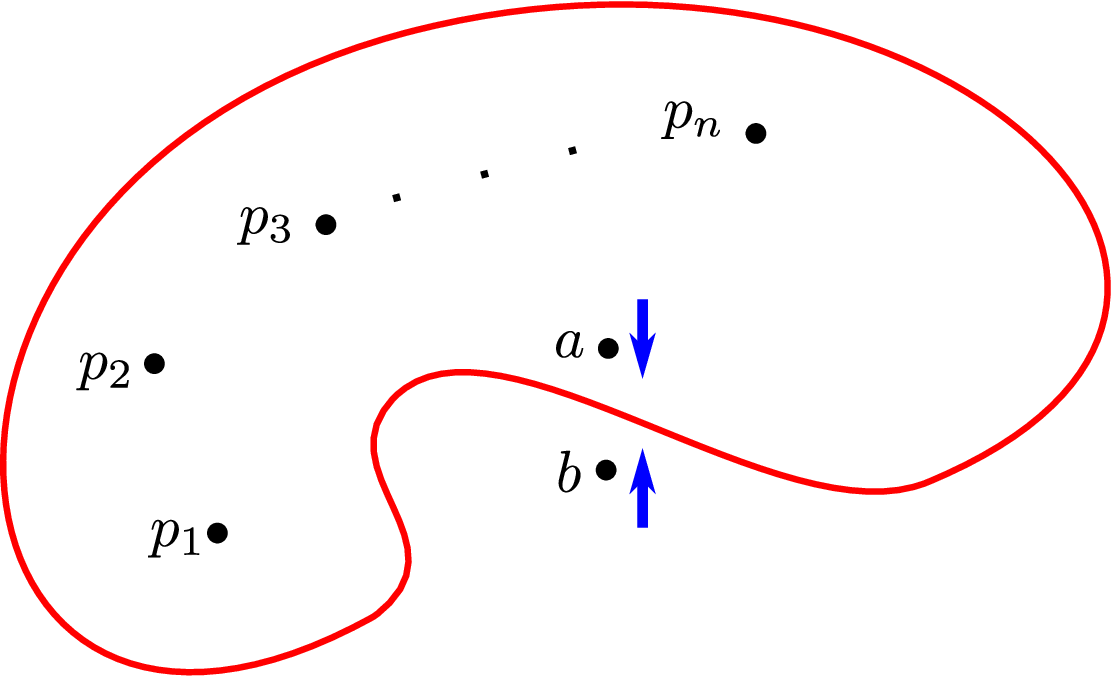
Refer to caption
Figure 8: The figure shows an example of contour pinching. As the poles at aa and at bb collide, the contour integral diverges, which is why we regulate it by multiplying with a−ba-b. In the limit a→ba\rightarrow b, the integral is given by a single residue.

If we now compute the contour integral of gg around 𝒞\mathcal{C} and multiply it by a−ba-b, we obtain

(a−b)​∮𝒞d​z2​π​i​g​(z)\displaystyle(a-b)\oint_{\mathcal{C}}\frac{dz}{2\pi i}g(z) =\displaystyle= f⁡(a)∏i(a−pi)+∑i(a−b)​f​(pi)(pi−a)​(pi−b)​∏j≠i(pi−pj)\displaystyle\frac{f(a)}{\prod_{i}(a-p_{i})}+\sum_{i}\frac{(a-b)f(p_{i})}{(p_{i}-a)(p_{i}-b)\prod_{j\neq i}(p_{i}-p_{j})} (51)
⟶δ→0\displaystyle\stackrel{{\scriptstyle\delta\rightarrow 0}}{{\longrightarrow}} f⁡(p)∏i(p−pi)=lima→b[(a−b)​Res​(g⁡(z),a)].\displaystyle\frac{f(p)}{\prod_{i}(p-p_{i})}=\lim_{a\rightarrow b}\left[(a-b)\text{Res}(g(z),a)\right]\,.

Thus, in the limit a→ba\rightarrow b, the contour gets pinched at the point a=b=pa=b=p and the integral is given by a single residue. This is essentially the contour integral version of the identity limε→0ε(x+i​ε)​(x−i​ε)=π​δ​(x)\lim_{\varepsilon\rightarrow 0}\frac{\varepsilon}{(x+i\varepsilon)(x-i\varepsilon)}=\pi\delta(x). This example can also be easily generalized to the case in which gg has not only simple poles, but we will not need it.

We now want to explain how this simple example applies to our integral formulas for the correlation functions of sl(3)(3).

Refer to caption
Figure 9: This figure shows the two flopping frames for T3T_{3}. One can obtain the right geometry from the left one by applying two flopping moves, see figure 7, to the encircled segments.

In the sl(3)(3) case, our contour integral formula (30) for the structure constants reads

Cq​(𝜶1,𝜶2,𝜶3)=const×∮d​A2​π​i​A​|M⁡(𝔱,𝔮)|2​|𝒵3top|2,C_{q}(\boldsymbol{\alpha}_{1},\boldsymbol{\alpha}_{2},\boldsymbol{\alpha}_{3})=\text{const}\times\oint\frac{d\textbf{A}}{2\pi i\textbf{A}}\left|M(\mathfrak{t},\mathfrak{q})\right|^{2}|\mathcal{Z}_{3}^{\text{top}}|^{2}\,, (52)

where A1(1)≡A=e−β​aA_{1}^{(1)}\equiv\textbf{A}=e^{-\beta\textbf{a}} while the integrand is

|𝒵3top|2=|𝒵3pert|2​|𝒵3inst|2=|∏1≤i<j≤3ℳ⁡(M~iM~j)∏k=13[ℳ(𝔱𝔮AM~kL~3)ℳ(𝔱𝔮AM~k​N~1)]​ℳ⁡(A2​L~3N~1)​ℳ​(N~1A2​L~3)ℳ⁡(𝔱𝔮​A​N~2L~1)​ℳ​(𝔱𝔮​A​N~3L~2)|2\displaystyle|\mathcal{Z}_{3}^{\text{top}}|^{2}=|\mathcal{Z}_{3}^{\text{pert}}|^{2}|\mathcal{Z}_{3}^{\text{inst}}|^{2}=\left|\frac{\prod_{1\leq i<j\leq 3}\mathcal{M}\left(\frac{\tilde{M}_{i}}{\tilde{M}_{j}}\right)}{\prod_{k=1}^{3}\biggl[\mathcal{M}\left(\sqrt{\frac{\mathfrak{t}}{\mathfrak{q}}}\textbf{A}\tilde{M}_{k}\tilde{L}_{3}\right)\mathcal{M}\left(\sqrt{\frac{\mathfrak{t}}{\mathfrak{q}}}\frac{\textbf{A}}{\tilde{M}_{k}\tilde{N}_{1}}\right)\biggl]}\frac{\mathcal{M}\left(\frac{\textbf{A}^{2}\tilde{L}_{3}}{\tilde{N}_{1}}\right)\mathcal{M}\left(\frac{\tilde{N}_{1}}{\textbf{A}^{2}\tilde{L}_{3}}\right)}{\mathcal{M}\left(\sqrt{\frac{\mathfrak{t}}{\mathfrak{q}}}\frac{\textbf{A}\tilde{N}_{2}}{\tilde{L}_{1}}\right)\mathcal{M}\left(\sqrt{\frac{\mathfrak{t}}{\mathfrak{q}}}\frac{\textbf{A}\tilde{N}_{3}}{\tilde{L}_{2}}\right)}\right|^{2}
×|∑𝝂(N~1​L~2N~2​L~3)|ν1(1)|+|ν2(1)|2(N~2​L~1N~3​L~2)|ν1(2)|2∏k=13[Nν1(1)​∅β​(a−mk−n1−Q/2)​N∅​ν2(1)β​(a+mk+l3−Q/2)]Nν1(1)​ν1(1)β​(0)​Nν2(1)​ν2(1)β​(0)​Nν1(2)​ν1(2)β​(0)\displaystyle\times\,\left|\sum_{\boldsymbol{\nu}}\,\left(\frac{\tilde{N}_{1}\tilde{L}_{2}}{\tilde{N}_{2}\tilde{L}_{3}}\right)^{\frac{|\nu_{1}^{(1)}|+|\nu_{2}^{(1)}|}{2}}\left(\frac{\tilde{N}_{2}\tilde{L}_{1}}{\tilde{N}_{3}\tilde{L}_{2}}\right)^{\frac{|\nu_{1}^{(2)}|}{2}}\frac{\prod_{k=1}^{3}\left[\textsf{N}^{\beta}_{\nu_{1}^{(1)}\emptyset}\left(\textbf{a}-m_{k}-n_{1}-\nicefrac{{Q}}{{2}}\right)\textsf{N}^{\beta}_{\emptyset\nu_{2}^{(1)}}\left(\textbf{a}+m_{k}+l_{3}-\nicefrac{{Q}}{{2}}\right)\right]}{\textsf{N}^{\beta}_{\nu_{1}^{(1)}\nu_{1}^{(1)}}\left(0\right)\textsf{N}^{\beta}_{\nu_{2}^{(1)}\nu_{2}^{(1)}}\left(0\right)\textsf{N}^{\beta}_{\nu_{1}^{(2)}\nu_{1}^{(2)}}\left(0\right)}\right.
×Nν1(1)​ν1(2)β​(a+n2−l1−Q/2)​Nν1(2)​ν2(1)β​(a+n3−l2−Q/2)Nν1(1)​ν2(1)β​(2​a−n1+l3)​Nν2(1)​ν1(1)β​(−2​a+n1−l3)|2,\displaystyle\times\,\left.\frac{\textsf{N}^{\beta}_{\nu_{1}^{(1)}\nu_{1}^{(2)}}\left(\textbf{a}+n_{2}-l_{1}-\nicefrac{{Q}}{{2}}\right)\textsf{N}^{\beta}_{\nu_{1}^{(2)}\nu_{2}^{(1)}}\left(\textbf{a}+n_{3}-l_{2}-\nicefrac{{Q}}{{2}}\right)}{\textsf{N}^{\beta}_{\nu_{1}^{(1)}\nu_{2}^{(1)}}\left(2\textbf{a}-n_{1}+l_{3}\right)\textsf{N}^{\beta}_{\nu_{2}^{(1)}\nu_{1}^{(1)}}\left(-2\textbf{a}+n_{1}-{l_{3}}\right)}\right|^{2}, (53)

with the sum going over all partitions 𝝂={ν1(1),ν2(1),ν1(2)}\boldsymbol{\nu}=\{\nu_{1}^{(1)},\nu_{2}^{(1)},\nu_{1}^{(2)}\}. Since we wish to evaluate the contour integral (52) in the semi-degenerate limit 𝜶1=3​ϰ​ω2\boldsymbol{\alpha}_{1}=3\varkappa\omega_{2}, we introduce a regulator δ\delta and parametrize the three masses labeling the positions of the branes on the left as

m1=ϰ+δ−Q,m2=ϰ−δ,m3=−2​ϰ+Q,m_{1}=\varkappa+\delta-Q\,,\qquad m_{2}=\varkappa-\delta\,,\qquad m_{3}=-2\varkappa+Q\,, (54)

which implies that the exponentiated masses M~i=e−β​mi\tilde{M}_{i}=e^{-\beta m_{i}} are

M~1=𝔱𝔮​K~​e−β​δ,M~2=K~​eβ​δ,M~3=𝔮𝔱​K~−2,\tilde{M}_{1}=\frac{\mathfrak{t}}{\mathfrak{q}}\tilde{K}e^{-\beta\delta}\,,\qquad\tilde{M}_{2}=\tilde{K}e^{\beta\delta}\,,\qquad\tilde{M}_{3}=\frac{\mathfrak{q}}{\mathfrak{t}}\tilde{K}^{-2}\,, (55)

with K~=e−β​ϰ\tilde{K}=e^{-\beta\varkappa}. The semi-degenerate limit then corresponds to δ→0\delta\rightarrow 0. For these values of the masses, the numerator of |𝒵3top|2|\mathcal{Z}_{3}^{\text{top}}|^{2} in (53) goes to zero, just like the term a−ba-b in the simple example (51) above, since

|ℳ⁡(M~1​M~2−1)|2=(1−e−2​β​δ)×reg.≈δ×reg.,|\mathcal{M}(\tilde{M}_{1}\tilde{M}_{2}^{-1})|^{2}=(1-e^{-2\beta\delta})\times\text{reg.}\approx\delta\times\text{reg.}\,, (56)

where “reg” are terms that don’t vanish for δ→0\delta\rightarrow 0.

The next step is to analyze the poles in the integrand of (53) and determine which ones will contribute in the semi-degenerate limit. We make the assumption1414 14 This can be supported by a following simple observation. The integral in our formula (16) for the Toda three-point function should be regarded as a complicated deformation of a conventional Mellin-Barnes contour integral of ratio of gamma functions multiplying a hypergeometric function. The “perturbative” part of the integrand corresponds to the deformed gamma functions, whereas the “instanton” part is the analogue of the hypergeometric function. As the usual hypergeometric function is an entire function of its parameters, it cannot give residue contributions to the value of the Mellin-Barnes integral. It is natural to expect the same property for its deformation. that only poles from the “perturbative” part, i.e. the first line of (53), are relevant for this computation, which will be justified by the final result.

Due to the vanishing of the numerator (56), we need to have pinching in order to get a non-zero answer. As we learned from the simple example at the beginning of the section, we need to find poles that lie on different sides of the contour and that collide when the regulator is removed. The poles in the integrand come from the zeroes of the functions |ℳ⁡(U)|2|\mathcal{M}(U)|^{2} in the first line of (53). Since, in order to obtain the Toda theory from topological strings we wish to have b>0b>0, so that |𝔮|<1|\mathfrak{q}|<1 and |𝔱|>1|\mathfrak{t}|>1, we get from (A.29) the expression

|ℳ⁡(U,𝔱,𝔮)|2=ℳ⁡(U,𝔱,𝔮)​ℳ​(U−1,𝔱−1,𝔮−1)=∏i,j=1∞(1−U​𝔱−i​𝔮j)​(1−U−1​𝔱1−i​𝔮j−1).|\mathcal{M}(U;\mathfrak{t},\mathfrak{q})|^{2}=\mathcal{M}(U;\mathfrak{t},\mathfrak{q})\mathcal{M}(U^{-1};\mathfrak{t}^{-1},\mathfrak{q}^{-1})=\prod_{i,j=1}^{\infty}(1-U\mathfrak{t}^{-i}\mathfrak{q}^{j})(1-U^{-1}\mathfrak{t}^{1-i}\mathfrak{q}^{j-1})\,. (57)

Thus, the zeroes of |ℳ⁡(U)|2|\mathcal{M}(U)|^{2} are to be found on the points

U=𝔱−m​𝔮n,U=𝔱m+1​𝔮−n−1,U=\mathfrak{t}^{-m}\mathfrak{q}^{n}\,,\qquad U=\mathfrak{t}^{m+1}\mathfrak{q}^{-n-1}\,, (58)

for m,n∈ℕ0={0,1,2,…}m,n\in\mathbb{N}_{0}=\{0,1,2,\ldots\}. We see that there are two classes of poles of |𝒵top|2|\mathcal{Z}^{\text{top}}|^{2}, namely those that condense around zero in the A complex plane and those that condense around infinity.

When we then take the limit δ→0\delta\rightarrow 0, some poles from the exterior of the contour integral with coincide with some from the interior, leading to a divergence that will cancel the zero of (57), just like in the simple example of equation (51). We easily see that the relevant terms in the denominator of the first line of (53) are

|ℳ⁡(𝔱𝔮​A​M~1−1​N~1−1)​ℳ​(𝔱𝔮​A​M~2−1​N~1−1)​ℳ​(𝔱𝔮​A​M~1​L~3)​ℳ​(𝔱𝔮​A​M~2​L~3)|2.\left|\mathcal{M}\left(\sqrt{\frac{\mathfrak{t}}{\mathfrak{q}}}\textbf{A}\tilde{M}_{1}^{-1}\tilde{N}_{1}^{-1}\right)\mathcal{M}\left(\sqrt{\frac{\mathfrak{t}}{\mathfrak{q}}}\textbf{A}\tilde{M}_{2}^{-1}\tilde{N}_{1}^{-1}\right)\mathcal{M}\left(\sqrt{\frac{\mathfrak{t}}{\mathfrak{q}}}\textbf{A}\tilde{M}_{1}\tilde{L}_{3}\right)\mathcal{M}\left(\sqrt{\frac{\mathfrak{t}}{\mathfrak{q}}}\textbf{A}\tilde{M}_{2}\tilde{L}_{3}\right)\right|^{2}\,. (59)

The other zeroes in the denominator will not pinch the integral once the regulator δ\delta is set to zero and can be ignored, just like the pip_{i} terms in (51). Numbering the functions ℳ\mathcal{M} as 11 to 44 in (59) from left to right, using (58) and the parametrization (54), we know that we have first order poles in the integrand if

(1)\displaystyle(1) A=K~​N~1​e−β​δ​𝔱−m+12​𝔮n−12,\displaystyle\textbf{A}=\tilde{K}\tilde{N}_{1}e^{-\beta\delta}\mathfrak{t}^{-m+\frac{1}{2}}\mathfrak{q}^{n-\frac{1}{2}}\,, (1¯)\displaystyle(\bar{1}) A=K~​N~1​e−β​δ​𝔱m+32​𝔮−n−32,\displaystyle\textbf{A}=\tilde{K}\tilde{N}_{1}e^{-\beta\delta}\mathfrak{t}^{m+\frac{3}{2}}\mathfrak{q}^{-n-\frac{3}{2}}\,,
(2)\displaystyle(2) A=K~​N~1​eβ​δ​𝔱−m−12​𝔮n+12,\displaystyle\textbf{A}=\tilde{K}\tilde{N}_{1}e^{\beta\delta}\mathfrak{t}^{-m-\frac{1}{2}}\mathfrak{q}^{n+\frac{1}{2}}\,, (2¯)\displaystyle(\bar{2}) A=K~​N~1​eβ​δ​𝔱m+12​𝔮−n−12,\displaystyle\textbf{A}=\tilde{K}\tilde{N}_{1}e^{\beta\delta}\mathfrak{t}^{m+\frac{1}{2}}\mathfrak{q}^{-n-\frac{1}{2}}\,,
(3)\displaystyle(3) A=K~−1​L~3−1​eβ​δ​𝔱−m−32​𝔮n+32,\displaystyle\textbf{A}=\tilde{K}^{-1}\tilde{L}_{3}^{-1}e^{\beta\delta}\mathfrak{t}^{-m-\frac{3}{2}}\mathfrak{q}^{n+\frac{3}{2}}\,, (3¯)\displaystyle(\bar{3}) A=K~−1​L~3−1​eβ​δ​𝔱m−12​𝔮−n+12,\displaystyle\textbf{A}=\tilde{K}^{-1}\tilde{L}_{3}^{-1}e^{\beta\delta}\mathfrak{t}^{m-\frac{1}{2}}\mathfrak{q}^{-n+\frac{1}{2}}\,,
(4)\displaystyle(4) A=K~−1​L~3−1​e−β​δ​𝔱−m−12​𝔮n+12,\displaystyle\textbf{A}=\tilde{K}^{-1}\tilde{L}_{3}^{-1}e^{-\beta\delta}\mathfrak{t}^{-m-\frac{1}{2}}\mathfrak{q}^{n+\frac{1}{2}}\,, (4¯)\displaystyle(\bar{4}) A=K~−1​L~3−1​e−β​δ​𝔱m+12​𝔮−n−12,\displaystyle\textbf{A}=\tilde{K}^{-1}\tilde{L}_{3}^{-1}e^{-\beta\delta}\mathfrak{t}^{m+\frac{1}{2}}\mathfrak{q}^{-n-\frac{1}{2}}\,, (60)

for m,n∈ℕ0m,n\in\mathbb{N}_{0}. We have labeled with a ⋅¯\bar{\cdot} those sets of poles that coalesce around A=∞\textbf{A}=\infty. We see in figure 10 that there are two places where the towers of poles collide, namely where the first pole of the tower 11 hits the first pole of the tower 2¯\bar{2} and where the first pole of the tower 33 hits the first of the tower 4¯\bar{4}. Now the time has come for us to choose the form of the contour. Given the fact that we need to pinch the contour, we have three possible options, depicted in  10. We will compute the integral for each of the three choices.

We begin with the first contour, see figure 10, passing between the towers 11 and 2¯\bar{2} but avoiding the pinching of the towers 33 and 4¯\bar{4}.

Refer to caption
Figure 10: As the variable δ\delta is sent to zero, the contour gets pinched between two zeroes and the contributions are given by finite number of residues, indicated by circles. The set of poles are labeled according to (60). The first contour picks up a single residue from the line of poles 11, the second one a single residue from the line of poles 33, while the third one, shown on the right, picks both of these residues.

We see that, due to set of poles 11 colliding with the set of poles 2¯\bar{2} for m=n=0m=n=0, the integral gets pinched as δ→0\delta\rightarrow 0 and that the result is given by the residue at

A=𝔱𝔮​K~​N~1​e−β​δ.\textbf{A}=\sqrt{\frac{\mathfrak{t}}{\mathfrak{q}}}\tilde{K}\tilde{N}_{1}e^{-\beta\delta}\,. (61)

It is very important as a guiding principle to note that this first contour corresponds to Higgsing in the flopping frame of figure 11.

Refer to caption
Figure 11: The figure shows the Higgsed geometry corresponding to the residue (61). For this residue, the Kähler parameters take the values (39).

We furthermore see that for the choice of contour in figure 10, the fact that for δ→0\delta\rightarrow 0 we get an overlap between a pole from 33 and a pole from 4¯\bar{4} is of no consequence since they both lie of the same side of the contour.

Let us now compute the residue of |𝒵3top|2|\mathcal{Z}^{\text{top}}_{3}|^{2} at (61) directly. We first need a couple of technical results. We can use the fact that for a function ff that has no pole at B​𝔱k​𝔮lB\mathfrak{t}^{k}\mathfrak{q}^{l}, we have

Res​(f⁡(A)A​|ℳ⁡(A​B−1)|2,A=B​𝔱k​𝔮l)=g−k,l|M⁡(𝔱,𝔮)|2​f​(B​𝔱k​𝔮l).\displaystyle\text{Res}\left(\frac{f(\textbf{A})}{\textbf{A}|\mathcal{M}(\textbf{A}B^{-1})|^{2}},\textbf{A}=B\mathfrak{t}^{k}\mathfrak{q}^{l}\right)=\frac{\textsf{g}_{-k,l}}{\left|M(\mathfrak{t},\mathfrak{q})\right|^{2}}f(B\mathfrak{t}^{k}\mathfrak{q}^{l})\,. (62)

Here |M⁡(𝔱,𝔮)|2\left|M(\mathfrak{t},\mathfrak{q})\right|^{2} is the norm squared of the refined MacMahon function defined in (A.40) and the function gk​l\textsf{g}_{kl} is defined as

gk​l(𝔱,𝔮):⁣=limU→1|ℳ⁡(U)|2|ℳ⁡(U​𝔱−k​𝔮l)|2=∏i=1k(𝔱−i​𝔮l+1,𝔮)∞(𝔱i​𝔮−l,𝔮)∞∏j=1l(𝔱−1​𝔮j,𝔱−1)∞(𝔮−j,𝔱−1)∞,\textsf{g}_{kl}(\mathfrak{t},\mathfrak{q})\mathrel{\mathchoice{\vbox{\hbox{$\displaystyle:$}}}{\vbox{\hbox{$\textstyle:$}}}{\vbox{\hbox{$\scriptstyle:$}}}{\vbox{\hbox{$\scriptscriptstyle:$}}}{=}}\lim_{U\rightarrow 1}\frac{\left|\mathcal{M}(U)\right|^{2}}{\left|\mathcal{M}(U\mathfrak{t}^{-k}\mathfrak{q}^{l})\right|^{2}}=\prod_{i=1}^{k}\frac{(\mathfrak{t}^{-i}\mathfrak{q}^{l+1};\mathfrak{q})_{\infty}}{(\mathfrak{t}^{i}\mathfrak{q}^{-l};\mathfrak{q})_{\infty}}\prod_{j=1}^{l}\frac{(\mathfrak{t}^{-1}\mathfrak{q}^{j};\mathfrak{t}^{-1})_{\infty}}{(\mathfrak{q}^{-j};\mathfrak{t}^{-1})_{\infty}}\,, (63)

where we have used the shift properties (A.33) of the ℳ\mathcal{M} functions and the last equality is only valid for k,l∈ℕ0k,l\in\mathbb{N}_{0}. The above expression can be continued for negative kk and ll with gk​l=−g−k−1,−l−1\textsf{g}_{kl}=-\textsf{g}_{-k-1,-l-1}. In particular g−n,0=g0,−n=0\textsf{g}_{-n,0}=\textsf{g}_{0,-n}=0 for n≥1n\geq 1. Thus, we can now finally write down the residue for the pole (61) using (62)

limδ→0∮d​A2​π​i​A​|M⁡(𝔱,𝔮)|2​|𝒵3top|2\displaystyle\lim_{\delta\rightarrow 0}\oint\frac{d\textbf{A}}{2\pi i\textbf{A}}\left|M(\mathfrak{t},\mathfrak{q})\right|^{2}|\mathcal{Z}_{3}^{\text{top}}|^{2} =|M⁡(𝔱,𝔮)|2​Res​(|𝒵3top|2,A=𝔱𝔮​K~​N~1​e−β​δ)\displaystyle=\left|M(\mathfrak{t},\mathfrak{q})\right|^{2}\text{Res}\left(|\mathcal{Z}_{3}^{\text{top}}|^{2},\textbf{A}=\sqrt{\frac{\mathfrak{t}}{\mathfrak{q}}}\tilde{K}\tilde{N}_{1}e^{-\beta\delta}\right) (64)
=|ℳ⁡(K~−3)|2|∏k=13ℳ⁡(N~k​L~4−kK~)|2|Zinst3|2|A=𝔱𝔮K~N~1.\displaystyle=\frac{\left|\mathcal{M}(\tilde{K}^{-3})\right|^{2}}{\left|\prod_{k=1}^{3}\mathcal{M}\big(\frac{\tilde{N}_{k}\tilde{L}_{4-k}}{\tilde{K}}\big)\right|^{2}}\left|Z^{\text{inst}}_{3}\right|^{2}_{\big|\textbf{A}=\sqrt{\frac{\mathfrak{t}}{\mathfrak{q}}}\tilde{K}\tilde{N}_{1}}\,.

One can observe that due to (A.48), the sum over ν1(1)\nu_{1}^{(1)} in |𝒵inst3|2|A=𝔱𝔮K~N~1\left|\mathcal{Z}^{\text{inst}}_{3}\right|^{2}_{\big|\textbf{A}=\sqrt{\frac{\mathfrak{t}}{\mathfrak{q}}}\tilde{K}\tilde{N}_{1}} drops out and we obtain the following result for the “instanton” partition function

(𝒵inst3)|A=𝔱𝔮K~N~1=∑ν1,ν2(N~2​L~1N~3​L~2)|ν1|2(N~1​L~2N~2​L~3)|ν2|2×Nν1​∅β​(n3+l1−ϰ)​Nν2​ν1β​(n2+l2−ϰ)​N∅​ν2β​(n1+l3−ϰ)Nν1​ν1β​(0)​Nν2​ν2β​(0),\left(\mathcal{Z}^{\text{inst}}_{3}\right)_{\big|\textbf{A}=\sqrt{\frac{\mathfrak{t}}{\mathfrak{q}}}\tilde{K}\tilde{N}_{1}}=\sum_{\nu_{1},\nu_{2}}\left(\frac{\tilde{N}_{2}\tilde{L}_{1}}{\tilde{N}_{3}\tilde{L}_{2}}\right)^{\frac{|\nu_{1}|}{2}}\left(\frac{\tilde{N}_{1}\tilde{L}_{2}}{\tilde{N}_{2}\tilde{L}_{3}}\right)^{\frac{|\nu_{2}|}{2}}\\ \times\frac{\textsf{N}^{\beta}_{\nu_{1}\emptyset}(n_{3}+l_{1}-\varkappa)\textsf{N}^{\beta}_{\nu_{2}\nu_{1}}(n_{2}+l_{2}-\varkappa)\textsf{N}^{\beta}_{\emptyset\nu_{2}}(n_{1}+l_{3}-\varkappa)}{\textsf{N}^{\beta}_{\nu_{1}\nu_{1}}(0)\textsf{N}^{\beta}_{\nu_{2}\nu_{2}}(0)}\,, (65)

where we denoted ν1(2)≡ν1\nu_{1}^{(2)}\equiv\nu_{1}, ν2(1)≡ν2\nu_{2}^{(1)}\equiv\nu_{2}.

Next, we also need to compute the the contour integral for the second contour, depicted in blue in figure 10. We find that the result is given by the residue of |𝒵3top|2\left|\mathcal{Z}_{3}^{\text{top}}\right|^{2} at

A=𝔮𝔱​K~−1​L~3−1​e−β​δ,\textbf{A}=\sqrt{\frac{\mathfrak{q}}{\mathfrak{t}}}\tilde{K}^{-1}\tilde{L}_{3}^{-1}e^{-\beta\delta}\,, (66)

which, together with (54) implies for δ→0\delta\rightarrow 0 the Higgsed geometry shown in figure 12.

Refer to caption
Figure 12: The figure shows the Higgsed geometry corresponding to the residue (66).

Computing the residue, we find that the “perturbative” contribution, i.e. the prefactor of |𝒵3inst|2\left|\mathcal{Z}_{3}^{\text{inst}}\right|^{2} in (65), is the same as before. Furthermore, we find after relabeling ν2(1)↔ν1(1)\nu_{2}^{(1)}\leftrightarrow\nu_{1}^{(1)} and using (A.49) that the “instanton” contribution in (65) is unchanged, i.e.

(𝒵3inst)|A=𝔱𝔮K~N~1=(𝒵3inst)|A=𝔮𝔱K~−1L~3−1.\left(\mathcal{Z}^{\text{inst}}_{3}\right)_{\big|\textbf{A}=\sqrt{\frac{\mathfrak{t}}{\mathfrak{q}}}\tilde{K}\tilde{N}_{1}}=\left(\mathcal{Z}^{\text{inst}}_{3}\right)_{\big|\textbf{A}=\sqrt{\frac{\mathfrak{q}}{\mathfrak{t}}}\tilde{K}^{-1}\tilde{L}_{3}^{-1}}\,. (67)

Finally, for the third contour, shown on the right hand side of figure 10, we simply find the sum of the results of contour one and two.

In order to complete the computation, we need to calculate the sum in (65) over the two remaining partitions. For this purpose, we shall use the following identity that we shall state in full generality in section 6 and prove in appendix B:

∑ν1,ν2(V1​U1​U2)|ν1|​(V2​U2​U3)|ν2|​Nν1​∅β​(u1−Q/2)​Nν2​ν1β​(u2−Q/2)​N∅​ν2β​(u3−Q/2)Nν1​ν1β​(0)​Nν2​ν2β​(0)\displaystyle\sum_{\nu_{1},\nu_{2}}\left(V_{1}\sqrt{U_{1}U_{2}}\right)^{|\nu_{1}|}\left(V_{2}\sqrt{U_{2}U_{3}}\right)^{|\nu_{2}|}\frac{\textsf{N}^{\beta}_{\nu_{1}\emptyset}\left(u_{1}-\nicefrac{{Q}}{{2}}\right)\textsf{N}^{\beta}_{\nu_{2}\nu_{1}}\left(u_{2}-\nicefrac{{Q}}{{2}}\right)\textsf{N}^{\beta}_{\emptyset\nu_{2}}\left(u_{3}-\nicefrac{{Q}}{{2}}\right)}{\textsf{N}^{\beta}_{\nu_{1}\nu_{1}}\left(0\right)\textsf{N}^{\beta}_{\nu_{2}\nu_{2}}\left(0\right)} (68)
=ℳ⁡(U1​V1)​ℳ​(𝔱𝔮​V1​U2)​ℳ​(U2​V2)​ℳ​(𝔱𝔮​V2​U3)​ℳ​(U1​V1​U2​V2)​ℳ​(𝔱𝔮​V1​U2​V2​U3)ℳ⁡(𝔱𝔮​V1)​ℳ​(𝔱𝔮​V2)​ℳ​(𝔱𝔮​U1​V1​U2)​ℳ​(𝔱𝔮​V1​U2​V2)​ℳ​(𝔱𝔮​U2​V2​U3)​ℳ​(𝔱𝔮​U1​V1​U2​V2​U3),\displaystyle=\frac{\mathcal{M}\big(U_{1}V_{1}\big)\mathcal{M}\big(\frac{\mathfrak{t}}{\mathfrak{q}}V_{1}U_{2}\big)\mathcal{M}\big(U_{2}V_{2}\big)\mathcal{M}\big(\frac{\mathfrak{t}}{\mathfrak{q}}V_{2}U_{3}\big)\mathcal{M}\big(U_{1}V_{1}U_{2}V_{2}\big)\mathcal{M}\big(\frac{\mathfrak{t}}{\mathfrak{q}}V_{1}U_{2}V_{2}U_{3}\big)}{\mathcal{M}\big(\sqrt{\frac{\mathfrak{t}}{\mathfrak{q}}}V_{1}\big)\mathcal{M}\big(\sqrt{\frac{\mathfrak{t}}{\mathfrak{q}}}V_{2}\big)\mathcal{M}\big(\sqrt{\frac{\mathfrak{t}}{\mathfrak{q}}}U_{1}V_{1}U_{2}\big)\mathcal{M}\big(\sqrt{\frac{\mathfrak{t}}{\mathfrak{q}}}V_{1}U_{2}V_{2}\big)\mathcal{M}\big(\sqrt{\frac{\mathfrak{t}}{\mathfrak{q}}}U_{2}V_{2}U_{3}\big)\mathcal{M}\big(\sqrt{\frac{\mathfrak{t}}{\mathfrak{q}}}U_{1}V_{1}U_{2}V_{2}U_{3}\big)},

where Ui:=e−β​uiU_{i}:=e^{-\beta u_{i}}. Upon making the following substitutions in (68)

Uk=𝔮𝔱​N~4−k​L~kK~,V1=𝔱𝔮​K~N~3​L~2,V2=𝔱𝔮​K~N~2​L~3,U_{k}=\sqrt{\frac{\mathfrak{q}}{\mathfrak{t}}}\frac{\tilde{N}_{4-k}\tilde{L}_{k}}{\tilde{K}},\qquad V_{1}=\sqrt{\frac{\mathfrak{t}}{\mathfrak{q}}}\frac{\tilde{K}}{\tilde{N}_{3}\tilde{L}_{2}},\qquad V_{2}=\sqrt{\frac{\mathfrak{t}}{\mathfrak{q}}}\frac{\tilde{K}}{\tilde{N}_{2}\tilde{L}_{3}}, (69)

where k=1,2,3k=1,2,3, we arrive at

(𝒵3inst)|A=𝔱𝔮K~N~1=ℳ⁡(L~1L~2)​ℳ​(L~2L~3)​ℳ​(L~1L~3)​ℳ​(𝔱𝔮​N~1N~2)​ℳ​(𝔱𝔮​N~2N~3)​ℳ​(𝔱𝔮​N~1N~3)ℳ⁡(N~1​L~1K~)​ℳ​(N~1​L~2K~)​ℳ​(N~2​L~1K~)​ℳ​(𝔱𝔮​K~N~2​L~3)​ℳ​(𝔱𝔮​K~N~3​L~2)​ℳ​(𝔱𝔮​K~N~3​L~3).\left(\mathcal{Z}^{\text{inst}}_{3}\right)_{\big|\textbf{A}=\sqrt{\frac{\mathfrak{t}}{\mathfrak{q}}}\tilde{K}\tilde{N}_{1}}=\frac{\mathcal{M}\big(\frac{\tilde{L}_{1}}{\tilde{L}_{2}}\big)\mathcal{M}\big(\frac{\tilde{L}_{2}}{\tilde{L}_{3}}\big)\mathcal{M}\big(\frac{\tilde{L}_{1}}{\tilde{L}_{3}}\big)\mathcal{M}\big(\frac{\mathfrak{t}}{\mathfrak{q}}\frac{\tilde{N}_{1}}{\tilde{N}_{2}}\big)\mathcal{M}\big(\frac{\mathfrak{t}}{\mathfrak{q}}\frac{\tilde{N}_{2}}{\tilde{N}_{3}}\big)\mathcal{M}\big(\frac{\mathfrak{t}}{\mathfrak{q}}\frac{\tilde{N}_{1}}{\tilde{N}_{3}}\big)}{\mathcal{M}\big(\frac{\tilde{N}_{1}\tilde{L}_{1}}{\tilde{K}}\big)\mathcal{M}\big(\frac{\tilde{N}_{1}\tilde{L}_{2}}{\tilde{K}}\big)\mathcal{M}\big(\frac{\tilde{N}_{2}\tilde{L}_{1}}{\tilde{K}}\big)\mathcal{M}\big(\frac{\mathfrak{t}}{\mathfrak{q}}\frac{\tilde{K}}{\tilde{N}_{2}\tilde{L}_{3}}\big)\mathcal{M}\big(\frac{\mathfrak{t}}{\mathfrak{q}}\frac{\tilde{K}}{\tilde{N}_{3}\tilde{L}_{2}}\big)\mathcal{M}\big(\frac{\mathfrak{t}}{\mathfrak{q}}\frac{\tilde{K}}{\tilde{N}_{3}\tilde{L}_{3}}\big)}. (70)

Inserting the above into (64), we arrive at

limδ→0∮d​A2​π​i​A​|M⁡(𝔱,𝔮)|2​|𝒵3top|2\displaystyle\lim_{\delta\rightarrow 0}\oint\frac{d\textbf{A}}{2\pi i\textbf{A}}\left|M(\mathfrak{t},\mathfrak{q})\right|^{2}|\mathcal{Z}_{3}^{\text{top}}|^{2} =\displaystyle= |ℳ⁡(K~−3)​∏1≤i<j≤3ℳ⁡(N~j/N~i)​ℳ​(L~i/L~j)|2|∏i,j=13ℳ⁡(N~i​L~j​K~−1)|2\displaystyle\,\frac{\left|\mathcal{M}(\tilde{K}^{-3})\prod_{1\leq i<j\leq 3}\mathcal{M}\left(\nicefrac{{\tilde{N}_{j}}}{{\tilde{N}_{i}}}\right)\mathcal{M}\left(\nicefrac{{\tilde{L}_{i}}}{{\tilde{L}_{j}}}\right)\right|^{2}}{\left|\prod_{i,j=1}^{3}\mathcal{M}(\tilde{N}_{i}\tilde{L}_{j}\tilde{K}^{-1})\right|^{2}} (71)
=\displaystyle= (1−q)φ3Λ2​Υq​(3​ϰ)​∏1≤i<j≤3Υq​(ni−nj)​Υq​(l4−i−l4−j)∏i,j=13Υq​(ϰ−ni−l4−j),\displaystyle\,\frac{(1-q)^{\varphi_{3}}}{\Lambda^{2}}\frac{\Upsilon_{q}(3\varkappa)\prod_{1\leq i<j\leq 3}\Upsilon_{q}(n_{i}-n_{j})\Upsilon_{q}(l_{4-i}-l_{4-j})}{\prod_{i,j=1}^{3}\Upsilon_{q}(\varkappa-n_{i}-l_{4-j})},

where we have used (A.34), (A.35) and defined the exponent

φ3\displaystyle\varphi_{3} =(Q2−3​ϰ)2+∑1≤i<j≤3[(Q2+nj−ni)2+(Q2+l4−j−l4−i)2]−∑i,j=13(Q2+ni+l4−j−ϰ)2\displaystyle=\left(\frac{Q}{2}-3\varkappa\right)^{2}+\sum_{1\leq i<j\leq 3}\left[\left(\frac{Q}{2}+n_{j}-n_{i}\right)^{2}+\left(\frac{Q}{2}+l_{4-j}-l_{4-i}\right)^{2}\right]-\sum_{i,j=1}^{3}\left(\frac{Q}{2}+n_{i}+l_{4-j}-\varkappa\right)^{2}
=2​Q​(3​ϰ+∑i=13i⁡(ni+l4−i))−Q22=−2​Q​(2​𝒬−∑i=13𝜶i,ρ)−Q22,\displaystyle=2Q\left(3\varkappa+\sum_{i=1}^{3}i(n_{i}+l_{4-i})\right)-\frac{Q^{2}}{2}=-2Q\left(2\mathbf{\mathcal{Q}}-\sum_{i=1}^{3}\boldsymbol{\alpha}_{i},\rho\right)-\frac{Q^{2}}{2}\,, (72)

where in the last line we have used our sl(3)(3) conventions, see appendix A.2 and equation (23). Now we employ (A.41) and rearrange the prefactors of (71) to obtain the qq-deformed W3 Fateev-Litvinov structure constants (14) in the form conjectured by [1]:

Cq​(3​ϰ​ω2,𝜶2,𝜶3)=\displaystyle C_{q}(3\varkappa\omega_{2},\boldsymbol{\alpha}_{2},\boldsymbol{\alpha}_{3})=
=(β​|M⁡(𝔱,𝔮)|2)2​((1−qb)2​b−1​(1−qb−1)2​b)(2​𝒬−∑i=13𝜶i,ρ)​limδ→0∮d​A2​π​i​A​|M⁡(𝔱,𝔮)|2​|𝒵3top|2\displaystyle=\left(\beta\left|M(\mathfrak{t},\mathfrak{q})\right|^{2}\right)^{2}\left(\big(1-q^{b}\big)^{2b^{-1}}\big(1-q^{b^{-1}}\big)^{2b}\right)^{\left(2\mathbf{\mathcal{Q}}-\sum_{i=1}^{3}\boldsymbol{\alpha}_{i},\rho\right)}\lim_{\delta\rightarrow 0}\oint\frac{d\textbf{A}}{2\pi i\textbf{A}}\left|M(\mathfrak{t},\mathfrak{q})\right|^{2}|\mathcal{Z}_{3}^{\text{top}}|^{2} (73)
=((1−qb)2​b−1​(1−qb−1)2​b(1−q)2​Q)(2​𝒬−∑i=13𝜶i,ρ)​Υq′​(0)2​Υq​(3​ϰ)​∏e>0Υq​((,,,))​Υq​((,,,))∏i,j=13Υq​(ϰ+(𝜶2−𝒬,hi)+(𝜶3−𝒬,hj)).\displaystyle=\left(\frac{\big(1-q^{b}\big)^{2b^{-1}}\big(1-q^{b^{-1}}\big)^{2b}}{(1-q)^{2Q}}\right)^{\left(2\mathbf{\mathcal{Q}}-\sum_{i=1}^{3}\boldsymbol{\alpha}_{i},\rho\right)}\frac{\Upsilon_{q}^{\prime}(0)^{2}\Upsilon_{q}(3\varkappa)\prod_{e>0}\Upsilon_{q}(\left(\mathbf{\mathcal{Q}}-\boldsymbol{\alpha}_{2},e\right))\Upsilon_{q}(\left(\mathbf{\mathcal{Q}}-\boldsymbol{\alpha}_{3},e\right))}{\prod_{i,j=1}^{3}\Upsilon_{q}(\varkappa+(\boldsymbol{\alpha}_{2}-\mathbf{\mathcal{Q}},\,h_{i})+(\boldsymbol{\alpha}_{3}-\mathbf{\mathcal{Q}},\,h_{j}))}\,.

Taking here the 4D limit q→1q\rightarrow 1 and reintroducing the cosmological constant dependence according to (15) leads to the Fateev-Litvinov formula (13) for N=3N=3. To conclude, we see that any of the three contours that we presented leads to the desired formula, up to a factor of two for the third one that should be absorbed in the proportionality constant.

6 The general WN\textbf{W}_{N} case

Having computed the structure constants for the W3 case in the previous section, we now want to turn our attention to the general case. Starting with W4, corresponding to the T4T_{4} gauge theory, one has to deal with multiple integrals and their residues. We relegate the investigation of the subtleties associated to those to appendix C.

We begin with the following conjecture concerning the choice of the contour. As we saw in the last section, there are multiple choices that we believe all lead to the same final result, up to a multiplicity factor. Hence, here we make the simplest possible choice of the contour, corresponding to the flopping frame of figure 2, which pinches at just one pole.

We parametrize the masses as follows

M~i=(𝔱𝔮)N+1−2​i2​K~​difor​i=1,…,N−1,M~N=(𝔮𝔱)N−12​1K~N−1,\tilde{M}_{i}=\left(\frac{\mathfrak{t}}{\mathfrak{q}}\right)^{\frac{N+1-2i}{2}}\tilde{K}d_{i}\qquad\text{for}\,\,\,i=1,\dots,N-1,\qquad\tilde{M}_{N}=\left(\frac{\mathfrak{q}}{\mathfrak{t}}\right)^{\frac{N-1}{2}}\frac{1}{\tilde{K}^{N-1}}, (74)

where the di=e−β​δid_{i}=e^{-\beta\delta_{i}} are regulators satisfying ∏i=1N−1di=1\prod_{i=1}^{N-1}d_{i}=1 and K~=e−β​ϰ\tilde{K}=e^{-\beta\varkappa}. The numerator of |𝒵top|2\left|\mathcal{Z}^{\text{top}}\right|^{2} has a zero of order (N−2)​(N−1)2\frac{(N-2)(N-1)}{2} in the limit δi→0\delta_{i}\rightarrow 0 since

∏1≤i<j≤N|ℳ⁡(M~iM~j)|2=reg×∏1≤i<j≤N−1|ℳ⁡((𝔱𝔮)j−i​didj)|2,\prod_{1\leq i<j\leq N}\Big|\mathcal{M}\Big(\frac{\tilde{M}_{i}}{\tilde{M}_{j}}\Big)\Big|^{2}=\text{reg}\times\prod_{1\leq i<j\leq N-1}\Big|\mathcal{M}\left(\Big(\frac{\mathfrak{t}}{\mathfrak{q}}\Big)^{j-i}\frac{d_{i}}{d_{j}}\right)\Big|^{2}\,, (75)

and |ℳ⁡((𝔱/𝔮)n)|2=0\left|\mathcal{M}\left(\big(\nicefrac{{\mathfrak{t}}}{{\mathfrak{q}}}\big)^{n}\right)\right|^{2}=0 for n≥0n\geq 0. These zeroes can all be canceled by divergences coming from the pinching of the (N−2)​(N−1)2\frac{(N-2)(N-1)}{2} integrals if we choose the contour carefully, see for instance figure 14 for an example in the T4T_{4} case. Thus the final answer is obtained by taking the residues in the integration variables A~i(j){\tilde{A}_{i}^{(j)}} at

A~i(j)=(𝔱𝔮)i⁡(N−i−j)2​K~i​∏k=1jN~k.\tilde{A}_{i}^{(j)}=\left(\frac{\mathfrak{t}}{\mathfrak{q}}\right)^{\frac{i(N-i-j)}{2}}\tilde{K}^{i}\prod_{k=1}^{j}\tilde{N}_{k}\,. (76)

Computing the residues, we obtain the result:

limδa→0∮∏i=1N−2∏j=1N−1−i[d​A~i(j)2​π​i​A~i(j)​|M⁡(𝔱,𝔮)|2]​|𝒵Ntop|2=\displaystyle\lim_{\delta_{a}\to 0}\oint\prod_{i=1}^{N-2}\prod_{j=1}^{N-1-i}\biggl[\frac{d\tilde{A}_{i}^{(j)}}{2\pi i\tilde{A}_{i}^{(j)}}|M(\mathfrak{t},\mathfrak{q})|^{2}\biggr]|\mathcal{Z}_{N}^{\text{top}}|^{2}=
=|ℳ⁡(K~−N)|2|∏k=1Nℳ⁡(N~k​L~N+1−kK~)|2×|∑ν1,…,νN−1[∏i=1N−1(N~N−i​L~iN~N−i+1​L~i+1)|νi|2]\displaystyle=\frac{\left|\mathcal{M}(\tilde{K}^{-N})\right|^{2}}{\left|\prod_{k=1}^{N}\mathcal{M}\big(\frac{\tilde{N}_{k}\tilde{L}_{N+1-k}}{\tilde{K}}\big)\right|^{2}}\,\times\Bigg|\sum_{\nu_{1},\dots,\nu_{N-1}}\biggl[\prod_{i=1}^{N-1}\left(\frac{\tilde{N}_{N-i}\tilde{L}_{i}}{\tilde{N}_{N-i+1}\tilde{L}_{i+1}}\right)^{\frac{|\nu_{i}|}{2}}\biggr] (77)
×Nν1​∅β​(nN+l1−ϰ)​[∏i=1N−2Nνi+1​νiβ​(nN−i+li+1−ϰ)]​N∅​νN−1β​(n1+lN−ϰ)∏i=1N−1Nνi​νiβ​(0)|2.\displaystyle\times\frac{\textsf{N}^{\beta}_{\nu_{1}\emptyset}\left(n_{N}+l_{1}-\varkappa\right)\biggl[\prod_{i=1}^{N-2}\textsf{N}^{\beta}_{\nu_{i+1}\nu_{i}}\left(n_{N-i}+l_{i+1}-\varkappa\right)\biggr]\textsf{N}^{\beta}_{\emptyset\nu_{N-1}}\left(n_{1}+l_{N}-\varkappa\right)}{\prod_{i=1}^{N-1}\textsf{N}^{\beta}_{\nu_{i}\nu_{i}}\left(0\right)}\Bigg|^{2}\,.

Here νi\nu_{i} for i=1,…,N−1i=1,\dots,N-1 denote the partitions corresponding to the N−1N-1 brane junctions not affected by Higgsing at the given pole. For our choice of flopping frame, see figure 2, these partitions are readily identified as νi:=νi(N−i)\nu_{i}:=\nu_{i}^{(N-i)}, i=1,…,N−1i=1,\dots,N-1, see figure 4 of [1] for the notation.

The remaining sums in (77) will be now performed by using the summation identity (B.18) proven in appendix B.2, which we reproduce here for convenience.

Theorem

∑ν1,…,νN−1[∏i=1N−1(Vi​Ui​Ui+1)|νi|Nνi​νiβ​(0)]​Nν1​∅β​(u1−ϵ+/2)​[∏i=1N−2Nνi+1​νiβ​(ui+1−ϵ+/2)]​N∅​νN−1β​(uN−ϵ+/2)==∏i=1N−1∏j=1N−iℳ⁡(∏s=ji+j−1Us​Vs)​ℳ​(𝔱𝔮​Ui+jUj⋅∏s=ji+j−1Us​Vs)ℳ⁡(𝔱𝔮​Ui+j​∏s=ji+j−1Us​Vs)​ℳ​(𝔱𝔮​1Uj​∏s=ji+j−1Us​Vs).\sum_{\nu_{1},\dots,\nu_{N-1}}\left[\prod_{i=1}^{N-1}\frac{\left(V_{i}\sqrt{U_{i}U_{i+1}}\right)^{|\nu_{i}|}}{\textsf{N}^{\beta}_{\nu_{i}\nu_{i}}\left(0\right)}\right]\textsf{N}^{\beta}_{\nu_{1}\emptyset}\left(u_{1}-\nicefrac{{\epsilon_{+}}}{{2}}\right)\left[\prod_{i=1}^{N-2}\textsf{N}^{\beta}_{\nu_{i+1}\nu_{i}}\left(u_{i+1}-\nicefrac{{\epsilon_{+}}}{{2}}\right)\right]\textsf{N}^{\beta}_{\emptyset\nu_{N-1}}\left(u_{N}-\nicefrac{{\epsilon_{+}}}{{2}}\right)=\\ =\prod_{i=1}^{N-1}\prod_{j=1}^{N-i}\frac{\mathcal{M}\big(\prod_{s=j}^{i+j-1}U_{s}V_{s}\big)\mathcal{M}\big(\frac{\mathfrak{t}}{\mathfrak{q}}\frac{U_{i+j}}{U_{j}}\cdot\prod_{s=j}^{i+j-1}U_{s}V_{s}\big)}{\mathcal{M}\big(\sqrt{\frac{\mathfrak{t}}{\mathfrak{q}}}U_{i+j}\prod_{s=j}^{i+j-1}U_{s}V_{s}\big)\mathcal{M}\big(\sqrt{\frac{\mathfrak{t}}{\mathfrak{q}}}\frac{1}{U_{j}}\prod_{s=j}^{i+j-1}U_{s}V_{s}\big)}. (78)

Setting the parameters here to be equal to

Ui=𝔮𝔱​N~N−i+1​L~iK~,Vj=𝔱𝔮​K~N~N−j+1​L~j+1,\displaystyle U_{i}=\sqrt{\frac{\mathfrak{q}}{\mathfrak{t}}}\frac{\tilde{N}_{N-i+1}\tilde{L}_{i}}{\tilde{K}}\,,\qquad V_{j}=\sqrt{\frac{\mathfrak{t}}{\mathfrak{q}}}\frac{\tilde{K}}{\tilde{N}_{N-j+1}\tilde{L}_{j+1}}\,, (79)

for i=1,⋯Ni=1,\cdots N and j=1,⋯N−1j=1,\cdots N-1, one straightforwardly obtains:

∑ν1,…,νN−1[∏i=1N−1(N~N−i​L~iN~N−i+1​L~i+1)|νi|2]\displaystyle\sum_{\nu_{1},\dots,\nu_{N-1}}\biggl[\prod_{i=1}^{N-1}\left(\frac{\tilde{N}_{N-i}\tilde{L}_{i}}{\tilde{N}_{N-i+1}\tilde{L}_{i+1}}\right)^{\frac{|\nu_{i}|}{2}}\biggr]
×Nν1​∅β​(nN+l1−ϰ)​[∏i=1N−2Nνi+1​νiβ​(nN−i+li+1−ϰ)]​N∅​νN−1β​(n1+lN−ϰ)∏i=1N−1Nνi​νiβ​(0)\displaystyle\times\frac{\textsf{N}^{\beta}_{\nu_{1}\emptyset}\left(n_{N}+l_{1}-\varkappa\right)\biggl[\prod_{i=1}^{N-2}\textsf{N}^{\beta}_{\nu_{i+1}\nu_{i}}\left(n_{N-i}+l_{i+1}-\varkappa\right)\biggr]\textsf{N}^{\beta}_{\emptyset\nu_{N-1}}\left(n_{1}+l_{N}-\varkappa\right)}{\prod_{i=1}^{N-1}\textsf{N}^{\beta}_{\nu_{i}\nu_{i}}\left(0\right)}
=∏1≤i<j≤Nℳ⁡(L~iL~j)​ℳ​(𝔱𝔮​N~N−j+1N~N−i+1)ℳ⁡(N~N−j+1​L~iK~)​ℳ​(𝔱𝔮​K~N~N−i+1​L~j).\displaystyle=\prod_{1\leq i<j\leq N}\frac{\mathcal{M}\big(\frac{\tilde{L}_{i}}{\tilde{L}_{j}}\big)\mathcal{M}\big(\frac{\mathfrak{t}}{\mathfrak{q}}\frac{\tilde{N}_{N-j+1}}{\tilde{N}_{N-i+1}}\big)}{\mathcal{M}\big(\frac{\tilde{N}_{N-j+1}\tilde{L}_{i}}{\tilde{K}}\big)\mathcal{M}\big(\frac{\mathfrak{t}}{\mathfrak{q}}\frac{\tilde{K}}{\tilde{N}_{N-i+1}\tilde{L}_{j}}\big)}\,. (80)

Substituting (80) in (77) and expressing everything in term of the Υq\Upsilon_{q} functions through formula (A.34) one obtains

limδa→0∮∏i=1N−2∏j=1N−1−i[d​A~i(j)2​π​i​A~i(j)​|M⁡(𝔱,𝔮)|2]​|𝒵Ntop|2=\displaystyle\lim_{\delta_{a}\to 0}\oint\prod_{i=1}^{N-2}\prod_{j=1}^{N-1-i}\biggl[\frac{d\tilde{A}_{i}^{(j)}}{2\pi i\tilde{A}_{i}^{(j)}}|M(\mathfrak{t},\mathfrak{q})|^{2}\biggr]|\mathcal{Z}_{N}^{\text{top}}|^{2}=
=(1−q)φNΛN−1​Υq​(N​ϰ)​∏1≤i<j≤N[Υq​(ni−nj)​Υq​(lN+1−i−lN+1−j)]∏i,j=1NΥq​(ϰ−ni−lN+1−j)\displaystyle=\frac{(1-q)^{\varphi_{N}}}{\Lambda^{N-1}}\frac{\Upsilon_{q}(N\varkappa)\prod_{1\leq i<j\leq N}[\Upsilon_{q}(n_{i}-n_{j})\Upsilon_{q}(l_{N+1-i}-l_{N+1-j})]}{\prod_{i,j=1}^{N}\Upsilon_{q}(\varkappa-n_{i}-l_{N+1-j})}\ (81)

where the exponent

φN=(Q2−N​ϰ)2+∑1≤i<j≤N[(Q2+nj−ni)2+(Q2+lN+1−j−lN+1−i)2]−∑i,j=1N(Q2+ni+lN+1−j−ϰ)2\begin{split}\varphi_{N}=&\left(\frac{Q}{2}-N\varkappa\right)^{2}+\sum_{1\leq i<j\leq N}\left[\left(\frac{Q}{2}+n_{j}-n_{i}\right)^{2}+\left(\frac{Q}{2}+l_{N+1-j}-l_{N+1-i}\right)^{2}\right]\\ &-\sum_{i,j=1}^{N}\left(\frac{Q}{2}+n_{i}+l_{N+1-j}-\varkappa\right)^{2}\end{split} (82)

after a little algebra simplifies into

φN=2​Q​(N⁡(N−1)2​ϰ+∑i=1Ni⁡(ni+lN+1−i))−N−14​Q2=−2​Q​(2​𝒬−∑i=13𝜶i,ρ)−N−14​Q2.\varphi_{N}=2Q\left(\frac{N(N-1)}{2}\varkappa+\sum_{i=1}^{N}i(n_{i}+l_{N+1-i})\right)-\frac{N-1}{4}Q^{2}=-2Q\left(2\mathbf{\mathcal{Q}}-\sum_{i=1}^{3}\boldsymbol{\alpha}_{i},\rho\right)-\frac{N-1}{4}Q^{2}\,. (83)

Now we will employ our sl(N)(N) conventions, see appendix A.2, equation (23) as well as equations (A.35), (A.41) and rearrange the prefactors to obtain the the qq-deformed Fateev-Litvinov 3-point function in the form conjectured by [1]:

Cq​(N​ϰ​ωN−1,𝜶2,𝜶3)=(β​|M⁡(𝔱,𝔮)|2)N−1​((1−qb)2​b−1​(1−qb−1)2​b)(2​𝒬−∑i=13𝜶i,ρ)\displaystyle C_{q}(N\varkappa\omega_{N-1},\boldsymbol{\alpha}_{2},\boldsymbol{\alpha}_{3})=\left(\beta\left|M(\mathfrak{t},\mathfrak{q})\right|^{2}\right)^{N-1}\left(\big(1-q^{b}\big)^{2b^{-1}}\big(1-q^{b^{-1}}\big)^{2b}\right)^{\left(2\mathbf{\mathcal{Q}}-\sum_{i=1}^{3}\boldsymbol{\alpha}_{i},\rho\right)}
×limδa→0∮∏i=1N−2∏j=1N−1−i[d​A~i(j)2​π​i​A~i(j)​|M⁡(𝔱,𝔮)|2]​|𝒵Ntop|2\displaystyle\qquad\qquad\qquad\qquad\qquad\times\lim_{\delta_{a}\to 0}\oint\prod_{i=1}^{N-2}\prod_{j=1}^{N-1-i}\biggl[\frac{d\tilde{A}_{i}^{(j)}}{2\pi i\tilde{A}_{i}^{(j)}}|M(\mathfrak{t},\mathfrak{q})|^{2}\biggr]|\mathcal{Z}_{N}^{\text{top}}|^{2} (84)
=((1−qb)2​b−1​(1−qb−1)2​b(1−q)2​Q)(2​𝒬−∑i=13𝜶i,ρ)​Υq′​(0)N−1​Υq​(N​ϰ)​∏e>0Υq​((,,,))​Υq​((,,,))∏i,j=1NΥq​(ϰ+(𝜶2−𝒬,hi)+(𝜶3−𝒬,hj)).\displaystyle=\left(\frac{\big(1-q^{b}\big)^{2b^{-1}}\big(1-q^{b^{-1}}\big)^{2b}}{(1-q)^{2Q}}\right)^{\left(2\mathbf{\mathcal{Q}}-\sum_{i=1}^{3}\boldsymbol{\alpha}_{i},\rho\right)}\frac{\Upsilon_{q}^{\prime}(0)^{N-1}\Upsilon_{q}(N\varkappa)\prod_{e>0}\Upsilon_{q}(\left(\mathbf{\mathcal{Q}}-\boldsymbol{\alpha}_{2},e\right))\Upsilon_{q}(\left(\mathbf{\mathcal{Q}}-\boldsymbol{\alpha}_{3},e\right))}{\prod_{i,j=1}^{N}\Upsilon_{q}(\varkappa+(\boldsymbol{\alpha}_{2}-\mathbf{\mathcal{Q}},\,h_{i})+(\boldsymbol{\alpha}_{3}-\mathbf{\mathcal{Q}},\,h_{j}))}\,.

Taking here the 4D limit q→1q\rightarrow 1 and reintroducing the cosmological constant dependence according to (15) leads to the Fateev-Litvinov formula (13) for general NN.

7 Conclusions and outlook

This paper is a second in the series of papers proposing a general formula (16) for primary 3-point functions of Toda CFT. Here we provided a very convincing check of (16) by reproducing an important known special case when one of the primaries has a null-vector at level one, a result due to Fateev and Litvinov [6]. Before giving an outlook of interesting problems we would like to be addressed next, let us briefly summarize the main points of this note.

After introducing a required background material, we discussed in section 4 how the degeneration of the primary fields on the Toda side corresponds to Higgsing on the (p,q)(p,q) 5-brane web diagram side. Committing to the choice of the flopping frame which then dictates the form of the contour, we demonstrated that, in the semi-degenerate limit, the contour integral expressing Toda structure constants is given by a single residue. This considerably simplified the flow of the subsequent calculation. Using a summation formula derived from qq-binomial identities (78) for Kaneko-Macdonald-Warnaar sl(n)(n) hypergeometric functions, we proved that the sums over partitions still present in the residues can be computed exactly. Eventually, our result (84) indeed gives the expression of Fateev and Litvinov (13) after one takes the q→1q\rightarrow 1 limit and reintroduces (15) the dependence on the cosmological constant μ\mu that is fixed from a corresponding Ward identity.

Reproducing the Fateev-Litvinov formula is a powerful test in support of our proposal for 3-point functions of generic Toda exponential fields. We would, of course, like to obtain further checks of (25) which is currently the work in progress. There are two natural steps to take here. The first one involves placing a more general semi-degenerate field to the 3-point function. Specifically for W3\textbf{W}_{3}, if a semi-degenerate condition reads 𝜶1=N​ϰ​ω2−m​b​ω1\boldsymbol{\alpha}_{1}=N\varkappa\omega_{2}-mb\omega_{1}, where mm is a positive integer, it corresponds to a primary field having a null-vector on a level m+1>1m+1>1. The Toda 3-point functions containing such a field are also known from [8]. In fact, these are the best of the CFT knowledge for the 3-point functions of generic primaries. The corresponding formula (see (3.11) and appendix B of [8]) involves two very different pieces: a straightforward generalization of (13) and a 4​m4m-dimensional Coulomb integral. This intriguing factorization indeed looks like to be reproducible from our general perspective.

The second natural step is matching the known semi-classical asymptotics [7]. We observe that in such a limit the combinatorial functions Nλ​μβ\textsf{N}^{\beta}_{\lambda\mu} factorize as

Nλ​μβ​(m,b,b−1)⟶b→∞Nλ​∅β​(m,b,b−1)​N∅​μβ​(m,b,b−1).\textsf{N}^{\beta}_{\lambda\mu}(m;b,b^{-1})\stackrel{{\scriptstyle b\rightarrow\infty}}{{\longrightarrow}}\textsf{N}^{\beta}_{\lambda\emptyset}(m;b,b^{-1})\textsf{N}^{\beta}_{\emptyset\mu}(m;b,b^{-1})\,. (85)

The sums over partitions thus disentangle, and proper generalizations of hypergeometric identities for the case of sl(2)(2) KM hypergeometric functions can be found to perform them. In fact, this step could then serve as a launch pad for a more ambitious goal of guessing a still unknown ’Lagrangian’ for the qq-deformed Toda theory. One would have to begin here by looking for the Lagrangian description of the qq-deformed Liouville theory, returning to the work of [21, 22]. It could well be that the 2D space has to be made non-commutative [51, 52, 53].

Having checked the known cases, it is very interesting to go beyond them, the ultimate goal being to compute the contour integral in (30) exactly for generic values of the parameters. This will mean a considerable simplification of our general formula for the 3-point functions of Toda primaries. Doing so requires finding a closed form expression for the “instanton” sum of (33), meaning that a suitable generalization of the KMW sl(n)(n) hypergeometric functions, as well as corresponding summation identities for them, have to be found. As an exercise to do before going for this serious problem, one could like to compute the corresponding sums for the cases with E6,7,8E_{6,7,8} flavor symmetry studied in [31, 13, 34, 35] which are obtained from the general TNT_{N} by a less severe Higgsing than the one we perform here.

Putting the above into the perspective of a full solution of the Toda theory, let us mention the remaining ingredients of it. First, a well-known fact is that, unlike the Virasoro case, the WN\textbf{W}_{N} symmetry is not restrictive enough to constrain the 3-point functions of descendent fields from those of primaries [54]. The number of corresponding Ward identities is simply too small to find from them the descendent structure constants. This means that in order to find all the 3-point correlators, one needs to calculate independently the 3-point structure constants of two primaries and one descendent. It is however rather straightforward from the topological strings point of view.

The second remaining ingredient of a complete solution of Toda CFT are the conformal blocks. The paper [55] describes the particular family of blocks which can be obtained by gluing the Fateev-Litvinov 3-point functions (13). Gluing the general (qq-deformed) Toda 3-point functions in the same way would give the general conformal blocks of the (qq-deformed) Toda CFT. Addressing this problem for qq-Liouville, that is a starting point in such an investigation, is the work in progress [56]. Due to many uncertainties in properly defining a qq-deformed Liouville (Toda) theory, such a finding would then as well work in opposite direction, allowing to know more about the qq-deformed AGT-W correspondence and its relation to topological strings (see [57]). The novel identities for Kaneko-Macdonald-Warnaar sl(n)(n) hypergeometric functions could probably be as helpful here as they were in the present note, to sum up known and new expressions for conformal blocks.

We finish with two remarks on the gauge theory side. The degeneration we study in this paper, and in general Higgsing, should also be understood on the 4D/5D gauge theory side using a generalization of the AGT correspondence with additional co-dimension two half-BPS surface defects [58] as in [59, 60, 61, 46]. See also [62, 63]. The partition functions with half-BPS surface operators can be obtained form certain 2D partition functions [64]. This 2D/4D relation has its qq-deformation to a 3D/5D relation that was initiated by [21] and further studied by [23, 22, 24]. See [65] for the latest advancements on the subject.

Lastly, by observing that the Higgsed geometry corresponding to the degeneration, see the right side of figure 2, is related to the strip geometry T~N\tilde{T}_{N}, see figure 7 in [11], by the Hanany-Witten effect. We refer the interested reader to [11, 66] for a nice discussion on the subject. The invariance of the topological string amplitude under the Hanany-Witten transition is non-trivial. It would be important to see how one can relate formula (14) for the qq-deformed structure constants to the topological string amplitude for the strip, see equation (4.66) of [12].

Acknowledgments

We would like to thank first our collaborators on closely related projects Masato Taki and Futoshi Yagi. We are indebted to Volker Schomerus and Futoshi Yagi for reading the draft of this paper and making helpful comments. In addition, we are thankful to Can Kozçaz, Fabrizio Nieri, Jörg Teschner and Dan Xie for insightful comments and discussions. We furthermore gratefully acknowledge support from the Simons Center for Geometry and Physics, Stony Brook University, as well as of the C.N. Yang Institute for Theoretical Physics, where some of the research for this paper was performed. V.M. acknowledges the support of the Marie Curie International Research Staff Exchange Network UNIFY of the European Union’s Seventh Framework Programme [FP7-People-2010-IRSES] under grant agreement n°269217, which allowed him to visit Stony Brook University. E.P. is partially supported by the Marie Curie action FP7-PEOPLE-2010-RG. M.I. thanks the Research Training Association RTG1670 for partial support. The research leading to these results has received funding from the People Programme (Marie Curie Actions) of the European Union’s Seventh Framework Programme FP7/2007-2013/ under REA Grant Agreement No 317089 (GATIS).

Appendix A Notations, conventions and special functions

In this appendix, we summarize our conventions and the main properties of the special functions that we use the most.

A.1 Parametrization of the TNT_{N} junction

Refer to caption
Figure 13: Parametrization for TNT_{N}. We denote the Kähler moduli parameters corresponding to the horizontal lines as Qn;i(j)Q_{n;i}^{(j)}, to the vertical lines as Ql;i(j)Q_{l;i}^{(j)}, and to tilted lines as Qm;i(j)Q_{m;i}^{(j)}. We denote the breathing modes as A~i(j)\tilde{A}^{(j)}_{i}. The index jj labels the strips in which the diagram can be decomposed.

We gather in this appendix all necessary formulas for the parametrizations of the Kähler moduli of the TNT_{N}. First, the “interior” Coulomb moduli A~j(i)=e−β​ai(j)\tilde{A}_{j}^{(i)}=e^{-\beta a_{i}^{(j)}} are independent, while the “border” ones are given by

A~i(0)=∏k=1iM~k,A~0(j)=∏k=1jN~k,A~i(N−i)=∏k=1iL~k.\tilde{A}_{i}^{(0)}=\prod_{k=1}^{i}\tilde{M}_{k},\qquad\tilde{A}_{0}^{(j)}=\prod_{k=1}^{j}\tilde{N}_{k},\qquad\tilde{A}_{i}^{(N-i)}=\prod_{k=1}^{i}\tilde{L}_{k}. (A.1)

The parameters labeling the positions of the flavors branes obey the relations

∏k=1NM~k=∏k=1NN~k=∏k=1NL~k=1⟺∑k=1Nmk=∑k=1Nnk=∑k=1Nlk=0.\prod_{k=1}^{N}\tilde{M}_{k}=\prod_{k=1}^{N}\tilde{N}_{k}=\prod_{k=1}^{N}\tilde{L}_{k}=1\Longleftrightarrow\sum_{k=1}^{N}m_{k}=\sum_{k=1}^{N}n_{k}=\sum_{k=1}^{N}l_{k}=0. (A.2)

Therefore, A~0(0)=A~N(0)=A~0(N)=1\tilde{A}_{0}^{(0)}=\tilde{A}_{N}^{(0)}=\tilde{A}_{0}^{(N)}=1 and we can invert relation (A.1) as

M~i=A~i(0)A~i−1(0),N~i=A~0(i)A~0(i−1),L~i=A~i(N−i)A~i−1(N−i+1).\tilde{M}_{i}=\frac{\tilde{A}_{i}^{(0)}}{\tilde{A}_{i-1}^{(0)}},\qquad\tilde{N}_{i}=\frac{\tilde{A}_{0}^{(i)}}{\tilde{A}_{0}^{(i-1)}},\qquad\tilde{L}_{i}=\frac{\tilde{A}_{i}^{(N-i)}}{\tilde{A}_{i-1}^{(N-i+1)}}. (A.3)

All placements are illustrated in figure 13. The Kähler parameters associated to the edges of the TNT_{N} junction are related to the A~i(j)\tilde{A}_{i}^{(j)} as follows

Qn;i(j)=A~i(j)​A~i−1(j)A~i(j−1)​A~i−1(j+1),Ql;i(j)=A~i(j)​A~i(j−1)A~i−1(j)​A~i+1(j−1),Qm;i(j)=A~i(j−1)​A~i−1(j)A~i(j)​A~i−1(j−1).\displaystyle Q_{n;i}^{(j)}=\frac{\tilde{A}_{i}^{(j)}\tilde{A}_{i-1}^{(j)}}{\tilde{A}_{i}^{(j-1)}\tilde{A}_{i-1}^{(j+1)}},\qquad Q_{l;i}^{(j)}=\frac{\tilde{A}_{i}^{(j)}\tilde{A}_{i}^{(j-1)}}{\tilde{A}_{i-1}^{(j)}\tilde{A}_{i+1}^{(j-1)}},\qquad Q_{m;i}^{(j)}=\frac{\tilde{A}_{i}^{(j-1)}\tilde{A}_{i-1}^{(j)}}{\tilde{A}_{i}^{(j)}\tilde{A}_{i-1}^{(j-1)}}. (A.4)

For each inner hexagon of (13), the following two constraints are satisfied

Ql;i(j)​Qm;i+1(j)=Qm;i(j+1)​Ql;i(j+1),Qn;i(j)​Qm;i(j+1)=Qm;i+1(j)​Qn;i+1(j).Q_{l;i}^{(j)}Q_{m;i+1}^{(j)}=Q_{m;i}^{(j+1)}Q_{l;i}^{(j+1)},\qquad Q_{n;i}^{(j)}Q_{m;i}^{(j+1)}=Q_{m;i+1}^{(j)}Q_{n;i+1}^{(j)}. (A.5)

A.2 Conventions and notations for SU​(N)\text{SU}(N)

For the convenience of the reader we summarize here our SU​(N)\text{SU}(N) conventions. The weights of the fundamental representation of SU​(N)\text{SU}(N) are hih_{i} with ∑i=1Nhi=0\sum_{i=1}^{N}h_{i}=0. We remind that the scalar product is defined via (hi,hj)=δi​j−1N\left(h_{i},h_{j}\right)=\delta_{ij}-\frac{1}{N}. The simple roots are

ek:⁣=hk−hk+1,k=1,…,N−1,e_{k}\mathrel{\mathchoice{\vbox{\hbox{$\displaystyle:$}}}{\vbox{\hbox{$\textstyle:$}}}{\vbox{\hbox{$\scriptstyle:$}}}{\vbox{\hbox{$\scriptscriptstyle:$}}}{=}}h_{k}-h_{k+1}\,,\qquad k=1,\ldots,N-1\,, (A.6)

and the positive roots e>0e>0 are contained in the set

Δ+:⁣={hi−hj}i<j=1N={ei}i=1N−1∪{ei+ei+1}i=1N−2∪⋯∪{e1+⋯+eN−1}.\Delta^{+}\mathrel{\mathchoice{\vbox{\hbox{$\displaystyle:$}}}{\vbox{\hbox{$\textstyle:$}}}{\vbox{\hbox{$\scriptstyle:$}}}{\vbox{\hbox{$\scriptscriptstyle:$}}}{=}}\{h_{i}-h_{j}\}_{i<j=1}^{N}=\{e_{i}\}_{i=1}^{N-1}\cup\{e_{i}+e_{i+1}\}_{i=1}^{N-2}\cup\cdots\cup\{e_{1}+\cdots+e_{N-1}\}\,. (A.7)

The Weyl vector ρ\rho for SU​(N)\text{SU}(N) is given by

ρ:⁣=12∑e>0e=12∑i<j=1N(hi−hj)=∑i=1NN+1−2​i2hi=ω1+⋯+ωN−1,\rho\mathrel{\mathchoice{\vbox{\hbox{$\displaystyle:$}}}{\vbox{\hbox{$\textstyle:$}}}{\vbox{\hbox{$\scriptstyle:$}}}{\vbox{\hbox{$\scriptscriptstyle:$}}}{=}}\frac{1}{2}\sum_{e>0}e=\frac{1}{2}\sum_{i<j=1}^{N}(h_{i}-h_{j})=\sum_{i=1}^{N}\frac{N+1-2i}{2}h_{i}=\omega_{1}+\cdots+\omega_{N-1}, (A.8)

and it obeys (ρ,ei)=1\left(\rho,e_{i}\right)=1 for all ii. The N−1N-1 fundamental weights ωi\omega_{i} of SU​(N)\text{SU}(N) are given by

ωi=∑k=1ihk,i=1,…,N−1\omega_{i}=\sum_{k=1}^{i}h_{k}\,,\qquad i=1,\dots,N-1 (A.9)

and the corresponding finite dimensional representations are the ii-fold antisymmetric tensor product of the fundamental representation. They obey the scalar products (ei,ωj)=δi​j\left(e_{i},\omega_{j}\right)=\delta_{ij}, i.e. they are a dual basis. Furthermore, we find the following scalar products useful

(ρ,hj)=N+12−j,(ρ,ωi)=i⁡(N−i)2,(hj,ωi)={1−iNj≤i−iNj>i,\left(\rho,h_{j}\right)=\frac{N+1}{2}-j,\qquad\left(\rho,\omega_{i}\right)=\frac{i(N-i)}{2},\qquad(h_{j},\omega_{i})=\left\{\begin{array}[]{ll}1-\frac{i}{N}&j\leq i\\ -\frac{i}{N}&j>i\end{array}\right.\,, (A.10)

as well as

(ωi,ωj)=min​(i,j)​(N−max​(i,j))N,(ρ,ρ)=N⁡(N2−1)12.\left(\omega_{i},\omega_{j}\right)=\frac{\text{min}(i,j)\left(N-\text{max}(i,j)\right)}{N},\qquad\left(\rho,\rho\right)=\frac{N(N^{2}-1)}{12}\,. (A.11)

The Weyl group of SU​(N)\text{SU}(N) is isomorphic to SNS_{N} and is generated by the N−1N-1 Weyl reflections associated to the simple roots. If 𝜶\boldsymbol{\alpha} is a weight, we define the Weyl reflections with respect to the simple root eie_{i}

𝗐i⋅𝜶:⁣=𝜶−2(ei,𝜶)(ei,ei)ei=𝜶−(ei,𝜶)ei.\mathsf{w}_{i}\cdot\boldsymbol{\alpha}\mathrel{\mathchoice{\vbox{\hbox{$\displaystyle:$}}}{\vbox{\hbox{$\textstyle:$}}}{\vbox{\hbox{$\scriptstyle:$}}}{\vbox{\hbox{$\scriptscriptstyle:$}}}{=}}\boldsymbol{\alpha}-2\frac{\left(e_{i},\boldsymbol{\alpha}\right)}{\left(e_{i},e_{i}\right)}e_{i}=\boldsymbol{\alpha}-\left(e_{i},\boldsymbol{\alpha}\right)e_{i}\,. (A.12)

Furthermore, we define the affine Weyl reflections with respect to eie_{i} as follows

𝗐i∘𝜶:⁣=𝒬+𝗐i⋅(𝜶−𝒬)=𝗐i⋅𝜶+Qei=𝜶−(𝜶−𝒬,ei)ei,\mathsf{w}_{i}\circ\boldsymbol{\alpha}\mathrel{\mathchoice{\vbox{\hbox{$\displaystyle:$}}}{\vbox{\hbox{$\textstyle:$}}}{\vbox{\hbox{$\scriptstyle:$}}}{\vbox{\hbox{$\scriptscriptstyle:$}}}{=}}\mathbf{\mathcal{Q}}+\mathsf{w}_{i}\cdot(\boldsymbol{\alpha}-\mathbf{\mathcal{Q}})=\mathsf{w}_{i}\cdot\boldsymbol{\alpha}+Qe_{i}=\boldsymbol{\alpha}-\left(\boldsymbol{\alpha}-\mathbf{\mathcal{Q}},e_{i}\right)e_{i}\,, (A.13)

where 𝒬:⁣=Qρ=(b+b−1)ρ\mathbf{\mathcal{Q}}\mathrel{\mathchoice{\vbox{\hbox{$\displaystyle:$}}}{\vbox{\hbox{$\textstyle:$}}}{\vbox{\hbox{$\scriptstyle:$}}}{\vbox{\hbox{$\scriptscriptstyle:$}}}{=}}Q\rho=(b+b^{-1})\rho.

A.3 Special functions

In this section we gather the definitions and properties of the special functions used in the main text.

We begin with the function Υ⁡(x)\Upsilon(x) which is defined for 0<ℜ⁡(x)<Q=b+b−10<\Re(x)<Q=b+b^{-1} as the integral

logΥ(x):⁣=∫0∞d​tt[(Q2−x)2e−t−sinh2⁡[(Q2−x)​t2]sinh⁡b​t2​sinh⁡t2​b].\log\Upsilon(x)\mathrel{\mathchoice{\vbox{\hbox{$\displaystyle:$}}}{\vbox{\hbox{$\textstyle:$}}}{\vbox{\hbox{$\scriptstyle:$}}}{\vbox{\hbox{$\scriptscriptstyle:$}}}{=}}\int_{0}^{\infty}\frac{dt}{t}\left[\left(\frac{Q}{2}-x\right)^{2}e^{-t}-\frac{\sinh^{2}\left[\left(\frac{Q}{2}-x\right)\frac{t}{2}\right]}{\sinh\frac{bt}{2}\sinh\frac{t}{2b}}\right]. (A.14)

It is clear from the definition that

Υ⁡(x)=Υ⁡(Q−x),Υ⁡(Q2)=1.\Upsilon(x)=\Upsilon(Q-x),\qquad\Upsilon\left(\frac{Q}{2}\right)=1. (A.15)

One can show from the alternative definition below that the following shift identities are obeyed

Υ⁡(x+b)=γ⁡(x​b)​b1−2​b​x​Υ​(x),Υ⁡(x+b−1)=γ⁡(x​b−1)​b2​x​b−1−1​Υ​(x).\Upsilon(x+b)=\gamma(xb)\,b^{1-2bx}\,\Upsilon(x),\qquad\Upsilon(x+b^{-1})=\gamma(xb^{-1})\,b^{2xb^{-1}-1}\,\Upsilon(x). (A.16)

where γ(x):⁣=Γ⁡(x)Γ⁡(1−x)\gamma(x)\mathrel{\mathchoice{\vbox{\hbox{$\displaystyle:$}}}{\vbox{\hbox{$\textstyle:$}}}{\vbox{\hbox{$\scriptstyle:$}}}{\vbox{\hbox{$\scriptscriptstyle:$}}}{=}}\frac{\Gamma(x)}{\Gamma(1-x)}. An useful implication is

Υ⁡(x+Q)=b2​(b−1−b)​x​Γ⁡(1+b​x)​Γ​(b−1​x)Γ⁡(1−b​x)​Γ​(−b−1​x)​Υ​(x),\Upsilon(x+Q)=b^{2(b^{-1}-b)x}\frac{\Gamma\big(1+bx\big)\Gamma\big(b^{-1}x\big)}{\Gamma\big(1-bx\big)\Gamma\big(-b^{-1}x\big)}\Upsilon(x), (A.17)

which is used in the derivation of the reflection amplitude (9). It follows from (A.16) that Υ\Upsilon is an entire function with zeroes at

x=−n1​b−n2​b−1, or x=(n1+1)​b+(n2+1)​b−1,x=-n_{1}b-n_{2}b^{-1},\quad\text{ or }\quad x=(n_{1}+1)b+(n_{2}+1)b^{-1}, (A.18)

where ni∈ℕ0n_{i}\in\mathbb{N}_{0}.

The function Υ\Upsilon can be connected to the Barnes Double Gamma function Γ2​(x|ω,ω2)\Gamma_{2}(x|\omega,\omega_{2}). First, we define Γ2​(x|ω1,ω2)\Gamma_{2}(x|\omega_{1},\omega_{2}) via the analytic continuation (the sum is only well-defined if ℜ⁡(t)>2\Re(t)>2) of

log⁡Γ2​(s|ω1,ω2)=[∂∂t​∑n1,n2=0∞(s+n1​ω1+n2​ω2)−t]t=0.\log\Gamma_{2}(s|\omega_{1},\omega_{2})=\left[\frac{\partial}{\partial t}\sum_{n_{1},n_{2}=0}^{\infty}(s+n_{1}\omega_{1}+n_{2}\omega_{2})^{-t}\right]_{t=0}. (A.19)

From this definition, one can prove (see A.54 of [67]) the difference property

Γ2​(s+ω1|ω1,ω2)Γ2​(s|ω1,ω2)=2​πω2sω2−12​Γ​(sω2),Γ2​(s+ω2|ω1,ω2)Γ2​(s|ω1,ω2)=2​πω1sω1−12​Γ​(sω1).\frac{\Gamma_{2}(s+\omega_{1}|\omega_{1},\omega_{2})}{\Gamma_{2}(s|\omega_{1},\omega_{2})}=\frac{\sqrt{2\pi}}{\omega_{2}^{\frac{s}{\omega_{2}}-\frac{1}{2}}\Gamma\Big(\frac{s}{\omega_{2}}\Big)},\qquad\frac{\Gamma_{2}(s+\omega_{2}|\omega_{1},\omega_{2})}{\Gamma_{2}(s|\omega_{1},\omega_{2})}=\frac{\sqrt{2\pi}}{\omega_{1}^{\frac{s}{\omega_{1}}-\frac{1}{2}}\Gamma\Big(\frac{s}{\omega_{1}}\Big)}. (A.20)

In order to express the Υ\Upsilon function using the Barnes double Gamma function, we have to first define the normalized function

Γb(x):⁣=Γ2​(x|b,b−1)Γ2​(Q2|b,b−1).\Gamma_{b}(x)\mathrel{\mathchoice{\vbox{\hbox{$\displaystyle:$}}}{\vbox{\hbox{$\textstyle:$}}}{\vbox{\hbox{$\scriptstyle:$}}}{\vbox{\hbox{$\scriptscriptstyle:$}}}{=}}\frac{\Gamma_{2}(x|b,b^{-1})}{\Gamma_{2}(\frac{Q}{2}|b,b^{-1})}. (A.21)

The log of the function Γb​(x)\Gamma_{b}(x) has an integral representation as

log⁡Γb​(x)=∫0∞d​tt​(e−x​t−e−Q​t2(1−e−t​b)​(1−e−t​b−1)−(Q2−x)22​e−t−Q2−xt).\log\Gamma_{b}(x)=\int_{0}^{\infty}\frac{dt}{t}\left(\frac{e^{-xt}-e^{-\frac{Qt}{2}}}{(1-e^{-tb})(1-e^{-tb^{-1}})}-\frac{\left(\frac{Q}{2}-x\right)^{2}}{2}e^{-t}-\frac{\frac{Q}{2}-x}{t}\right). (A.22)

Then, using (A.21) we can express the Υ⁡(x)\Upsilon(x) as

Υ⁡(x)=1Γb​(x)​Γb​(Q−x).\Upsilon(x)=\frac{1}{\Gamma_{b}(x)\Gamma_{b}(Q-x)}. (A.23)

This, together with the difference properties of Γ2\Gamma_{2} proves the shift identities (A.16).

We proceed by defining some qq-deformed special functions we need in the main text, such as shifted factorials1515 15 A good source for the properties of the shifted factorials is [68].

(U,q)p:=∏i=1p(1−U​qi−1)(U;q)_{p}:=\prod_{i=1}^{p}(1-Uq^{i-1}) (A.24)

for positive pp, which is continued to negative pp according to

(U,q)p=1(U​qp,q)−p.(U;q)_{p}=\frac{1}{(Uq^{p};q)_{-p}}\,. (A.25)

In particular for p→∞p\rightarrow\infty, and for arbitrary number of qq’s, we have (we require for convergence that |qi|<1|q_{i}|<1 for all ii)

(U;q1,…,qr)∞:⁣=∏i1=0,…,ir=0∞(1−Uq1i1⋯qrir).(U;q_{1},\ldots,q_{r})_{\infty}\mathrel{\mathchoice{\vbox{\hbox{$\displaystyle:$}}}{\vbox{\hbox{$\textstyle:$}}}{\vbox{\hbox{$\scriptstyle:$}}}{\vbox{\hbox{$\scriptscriptstyle:$}}}{=}}\prod_{i_{1}=0,\ldots,i_{r}=0}^{\infty}(1-Uq_{1}^{i_{1}}\cdots q_{r}^{i_{r}})\,. (A.26)

We can extend the definition of the shifted factorial for all values of qiq_{i} by imposing the relations

(U,q1,…,qi−1,…,qr)∞=1(U​qi,q1,…,qr)∞.(U;q_{1},\ldots,q_{i}^{-1},\ldots,q_{r})_{\infty}=\frac{1}{(Uq_{i};q_{1},\ldots,q_{r})_{\infty}}\,. (A.27)

Furthermore, they obey the following shifting properties

(qj​U,q1,…,qr)∞=(U,q1,…,qr)∞(U,q1,…,qj−1,qj+1,…,qr)∞.(q_{j}U;q_{1},\ldots,q_{r})_{\infty}=\frac{(U;q_{1},\ldots,q_{r})_{\infty}}{(U;q_{1},\ldots,q_{j-1},q_{j+1},\ldots,q_{r})_{\infty}}\,. (A.28)

We then define the function ℳ⁡(U,𝔱,𝔮)\mathcal{M}(U;\mathfrak{t},\mathfrak{q}) as

ℳ(U;𝔱,𝔮):⁣=(U𝔮;𝔱,𝔮)∞−1={∏i,j=1∞(1−U​𝔱i−1​𝔮j)−1 for ​|𝔱|<1,|𝔮|<1∏i,j=1∞(1−U​𝔱i−1​𝔮1−j) for ​|𝔱|​<1,|𝔮|>​1∏i,j=1∞(1−U​𝔱−i​𝔮j) for ​|𝔱|>1,|𝔮|<1∏i,j=1∞(1−U​𝔱−i​𝔮1−j)−1 for ​|𝔱|>1,|𝔮|>1,\mathcal{M}(U;\mathfrak{t},\mathfrak{q})\mathrel{\mathchoice{\vbox{\hbox{$\displaystyle:$}}}{\vbox{\hbox{$\textstyle:$}}}{\vbox{\hbox{$\scriptstyle:$}}}{\vbox{\hbox{$\scriptscriptstyle:$}}}{=}}(U\mathfrak{q};\mathfrak{t},\mathfrak{q})_{\infty}^{-1}=\left\{\begin{array}[]{ll}\prod_{i,j=1}^{\infty}(1-U\mathfrak{t}^{i-1}\mathfrak{q}^{j})^{-1}&\text{ for }|\mathfrak{t}|<1,|\mathfrak{q}|<1\\ \prod_{i,j=1}^{\infty}(1-U\mathfrak{t}^{i-1}\mathfrak{q}^{1-j})&\text{ for }|\mathfrak{t}|<1,|\mathfrak{q}|>1\\ \prod_{i,j=1}^{\infty}(1-U\mathfrak{t}^{-i}\mathfrak{q}^{j})&\text{ for }|\mathfrak{t}|>1,|\mathfrak{q}|<1\\ \prod_{i,j=1}^{\infty}(1-U\mathfrak{t}^{-i}\mathfrak{q}^{1-j})^{-1}&\text{ for }|\mathfrak{t}|>1,|\mathfrak{q}|>1\\ \end{array}\right.\,, (A.29)

converging for all UU. This function can be written as a plethystic exponential

ℳ⁡(U,𝔱,𝔮)=exp⁡[∑m=1∞Umm​𝔮m(1−𝔱m)​(1−𝔮m)],\mathcal{M}(U;\mathfrak{t},\mathfrak{q})=\exp\left[\sum_{m=1}^{\infty}\frac{U^{m}}{m}\frac{\mathfrak{q}^{m}}{(1-\mathfrak{t}^{m})(1-\mathfrak{q}^{m})}\right]\,, (A.30)

which converges for all 𝔱\mathfrak{t} and all 𝔮\mathfrak{q} provided that |U|<𝔮−1+θ⁡(|𝔮|−1)​𝔱θ⁡(|𝔱|−1)|U|<\mathfrak{q}^{-1+\theta(|\mathfrak{q}|-1)}\mathfrak{t}^{\theta(|\mathfrak{t}|-1)}. Here and elsewhere θ⁡(x)=1\theta(x)=1 if x>0x>0 and is zero otherwise. The following identity is obvious from the definition

ℳ⁡(U,𝔮,𝔱)=ℳ⁡(U​𝔱/𝔮,𝔱,𝔮).\mathcal{M}(U;\mathfrak{q},\mathfrak{t})=\mathcal{M}(U\nicefrac{{\mathfrak{t}}}{{\mathfrak{q}}};\mathfrak{t},\mathfrak{q})\,. (A.31)

From the analytic properties of the shifted factorials (A.27), we read the identities

ℳ⁡(U,𝔱−1,𝔮)=1ℳ⁡(U​𝔱,𝔱,𝔮),ℳ⁡(U,𝔱,𝔮−1)=1ℳ⁡(U​𝔮−1,𝔱,𝔮),\mathcal{M}(U;\mathfrak{t}^{-1},\mathfrak{q})=\frac{1}{\mathcal{M}(U\mathfrak{t};\mathfrak{t},\mathfrak{q})},\qquad\mathcal{M}(U;\mathfrak{t},\mathfrak{q}^{-1})=\frac{1}{\mathcal{M}(U\mathfrak{q}^{-1};\mathfrak{t},\mathfrak{q})}\,, (A.32)

while from (A.28) we take the following shifting identities

ℳ⁡(U​𝔱,𝔱,𝔮)=(U​𝔮,𝔮)∞​ℳ​(U,𝔱,𝔮),ℳ⁡(U​𝔮,𝔱,𝔮)=(U​𝔮,𝔱)∞​ℳ​(U,𝔱,𝔮).\mathcal{M}(U\mathfrak{t};\mathfrak{t},\mathfrak{q})=(U\mathfrak{q};\mathfrak{q})_{\infty}\mathcal{M}(U;\mathfrak{t},\mathfrak{q}),\qquad\mathcal{M}(U\mathfrak{q};\mathfrak{t},\mathfrak{q})=(U\mathfrak{q};\mathfrak{t})_{\infty}\mathcal{M}(U;\mathfrak{t},\mathfrak{q})\,. (A.33)

We define the qq-deformed Υ\Upsilon function as

Υq​(x|ϵ1,ϵ2)=(1−q)−1ϵ1​ϵ2​(x−ϵ+2)2​∏n1,n2=0∞(1−qx+n1​ϵ1+n2​ϵ2)​(1−qϵ+−x+n1​ϵ1+n2​ϵ2)(1−qϵ+/2+n1​ϵ1+n2​ϵ2)2=(1−q)−1ϵ1​ϵ2​(x−ϵ+2)2​|ℳ⁡(q−x,𝔱,𝔮)ℳ⁡(𝔱𝔮,𝔱,𝔮)|2,\begin{split}\Upsilon_{q}(x|\epsilon_{1},\epsilon_{2})=&(1-q)^{-\frac{1}{\epsilon_{1}\epsilon_{2}}\left(x-\frac{\epsilon_{+}}{2}\right)^{2}}\prod_{n_{1},n_{2}=0}^{\infty}\frac{(1-q^{x+n_{1}\epsilon_{1}+n_{2}\epsilon_{2}})(1-q^{\epsilon_{+}-x+n_{1}\epsilon_{1}+n_{2}\epsilon_{2}})}{(1-q^{\nicefrac{{\epsilon_{+}}}{{2}}+n_{1}\epsilon_{1}+n_{2}\epsilon_{2}})^{2}}\\ =&(1-q)^{-\frac{1}{\epsilon_{1}\epsilon_{2}}\left(x-\frac{\epsilon_{+}}{2}\right)^{2}}\left|\frac{\mathcal{M}(q^{-x};\mathfrak{t},\mathfrak{q})}{\mathcal{M}(\sqrt{\frac{\mathfrak{t}}{\mathfrak{q}}};\mathfrak{t},\mathfrak{q})}\right|^{2}\,,\end{split} (A.34)

where we have used the definition (29) for the norm squared. From time to time we will use the short-hand notation

Λ:⁣=|ℳ(𝔱𝔮;𝔱,𝔮)|2.\Lambda\mathrel{\mathchoice{\vbox{\hbox{$\displaystyle:$}}}{\vbox{\hbox{$\textstyle:$}}}{\vbox{\hbox{$\scriptstyle:$}}}{\vbox{\hbox{$\scriptscriptstyle:$}}}{=}}\left|\mathcal{M}\left(\sqrt{\frac{\mathfrak{t}}{\mathfrak{q}}};\mathfrak{t},\mathfrak{q}\right)\right|^{2}\,. (A.35)

If follows from the definition (A.34) that Υq​(ϵ+/2|ϵ1,ϵ2)=1\Upsilon_{q}(\nicefrac{{\epsilon_{+}}}{{2}}|\epsilon_{1},\epsilon_{2})=1, that Υq​(x|ϵ1,ϵ2)=Υq​(ϵ+−x|ϵ1,ϵ2)\Upsilon_{q}(x|\epsilon_{1},\epsilon_{2})=\Upsilon_{q}(\epsilon_{+}-x|\epsilon_{1},\epsilon_{2}) and that Υq​(x|ϵ1,ϵ2)=Υq​(x|ϵ2,ϵ1)\Upsilon_{q}(x|\epsilon_{1},\epsilon_{2})=\Upsilon_{q}(x|\epsilon_{2},\epsilon_{1}). Furthermore, from the shifting identities for ℳ\mathcal{M}, we can easily prove that

Υq​(x+ϵ1|ϵ1,ϵ2)=(1−q1−qϵ2)1−2​ϵ2−1​x​γqϵ2​(x​ϵ2−1)​Υq​(x|ϵ1,ϵ2),\Upsilon_{q}(x+\epsilon_{1}|\epsilon_{1},\epsilon_{2})=\left(\frac{1-q}{1-q^{\epsilon_{2}}}\right)^{1-2\epsilon_{2}^{-1}x}\gamma_{q^{\epsilon_{2}}}(x\epsilon_{2}^{-1})\Upsilon_{q}(x|\epsilon_{1},\epsilon_{2})\,, (A.36)

together with a similar equation for the shift with ϵ2\epsilon_{2}. Here, we have used the definition of the qq-deformed Γ\Gamma and γ\gamma functions

Γq(x):⁣=(1−q)1−x(q,q)∞(qx,q)∞,γq(x):⁣=Γq​(x)Γq​(1−x)=(1−q)1−2​x(q1−x,q)∞(qx,q)∞,\Gamma_{q}(x)\mathrel{\mathchoice{\vbox{\hbox{$\displaystyle:$}}}{\vbox{\hbox{$\textstyle:$}}}{\vbox{\hbox{$\scriptstyle:$}}}{\vbox{\hbox{$\scriptscriptstyle:$}}}{=}}(1-q)^{1-x}\frac{(q;q)_{\infty}}{(q^{x};q)_{\infty}},\qquad\gamma_{q}(x)\mathrel{\mathchoice{\vbox{\hbox{$\displaystyle:$}}}{\vbox{\hbox{$\textstyle:$}}}{\vbox{\hbox{$\scriptstyle:$}}}{\vbox{\hbox{$\scriptscriptstyle:$}}}{=}}\frac{\Gamma_{q}(x)}{\Gamma_{q}(1-x)}=(1-q)^{1-2x}\frac{(q^{1-x};q)_{\infty}}{(q^{x};q)_{\infty}}\,, (A.37)

valid for |q|<1|q|<1. They obey Γq​(x+1)=1−qx1−q​Γq​(x)\Gamma_{q}(x+1)=\frac{1-q^{x}}{1-q}\Gamma_{q}(x), implying γq​(x+1)=(1−qx)​(1−q−x)(1−q)2​γq​(x)\gamma_{q}(x+1)=\frac{(1-q^{x})(1-q^{-x})}{(1-q)^{2}}\gamma_{q}(x). Because of the normalization of Υq​(x|ϵ1,ϵ2)\Upsilon_{q}(x|\epsilon_{1},\epsilon_{2}) and since the factors of the right hand side of (A.36) have a well defined limit for q→1q\rightarrow 1, we find by comparing functional identities that

Υq(x|ϵ1,ϵ2)⟶q→1Υ(x|ϵ1,ϵ2):⁣=Γ2​(ϵ+2|ϵ1,ϵ2)2Γ2​(x|ϵ1,ϵ2)​Γ2​(ϵ+−x|ϵ1,ϵ2).\Upsilon_{q}({x}|\epsilon_{1},\epsilon_{2})\stackrel{{\scriptstyle q\rightarrow 1}}{{\longrightarrow}}\Upsilon(x|\epsilon_{1},\epsilon_{2})\mathrel{\mathchoice{\vbox{\hbox{$\displaystyle:$}}}{\vbox{\hbox{$\textstyle:$}}}{\vbox{\hbox{$\scriptstyle:$}}}{\vbox{\hbox{$\scriptscriptstyle:$}}}{=}}\frac{\Gamma_{2}\big(\frac{\epsilon_{+}}{2}|\epsilon_{1},\epsilon_{2}\big)^{2}}{\Gamma_{2}\big(x|\epsilon_{1},\epsilon_{2}\big)\Gamma_{2}\big(\epsilon_{+}-x|\epsilon_{1},\epsilon_{2}\big)}\,. (A.38)

where Γ2\Gamma_{2} is the Barnes Double Gamma function. In particular, the usual function Υ⁡(x)\Upsilon(x) introduced in [4] is equal to Υ⁡(x|b,b−1)\Upsilon(x|b,b^{-1}). We shall often just write Υq​(x)\Upsilon_{q}(x) instead of Υq​(x|ϵ1,ϵ2)\Upsilon_{q}(x|\epsilon_{1},\epsilon_{2}) and indicate in the text whether the ϵi\epsilon_{i} parameters are arbitrary or whether b=ϵ1=ϵ2−1b=\epsilon_{1}=\epsilon_{2}^{-1}.

We will also need to evaluate the derivative of Υq​(x)\Upsilon_{q}(x) at x=0x=0. Since the zero of Υq​(x)\Upsilon_{q}(x) at x=0x=0 is due to the factor (1−qx)(1-q^{x}) in the numerator of (A.34), we find that the only piece of the derivative that survives is

Υq′​(0)=β1−q​Υq​(b).\Upsilon_{q}^{\prime}(0)=\frac{\beta}{1-q}\Upsilon_{q}(b)\,. (A.39)

From this formula we can then obtain an identity useful for the calculations of the main text. Let us define the norm squared of the refined McMahon function following [29]:

|M⁡(𝔱,𝔮)|2:⁣=limU→1|ℳ⁡(U,𝔱,𝔮)|21−U−1=|ℳ(𝔮−1;𝔱,𝔮)|2=(1−q)(ϵ1−ϵ2)24​ϵ1​ϵ2ΛΥq(ϵ1).\begin{split}|M(\mathfrak{t},\mathfrak{q})|^{2}&\mathrel{\mathchoice{\vbox{\hbox{$\displaystyle:$}}}{\vbox{\hbox{$\textstyle:$}}}{\vbox{\hbox{$\scriptstyle:$}}}{\vbox{\hbox{$\scriptscriptstyle:$}}}{=}}\lim_{U\rightarrow 1}\frac{|\mathcal{M}(U;\mathfrak{t},\mathfrak{q})|^{2}}{1-U^{-1}}=|\mathcal{M}(\mathfrak{q}^{-1};\mathfrak{t},\mathfrak{q})|^{2}=(1-q)^{\frac{\left(\epsilon_{1}-\epsilon_{2}\right)^{2}}{4\epsilon_{1}\epsilon_{2}}}\Lambda\Upsilon_{q}(\epsilon_{1})\,.\end{split} (A.40)

Then, from (A.35) and (A.39) we get for ϵ1=b\epsilon_{1}=b and ϵ2=b−1\epsilon_{2}=b^{-1}

|M⁡(𝔱,𝔮)|2=1β​(1−q)(Q2)2​Λ​Υq′​(0).\left|M(\mathfrak{t},\mathfrak{q})\right|^{2}=\frac{1}{\beta}(1-q)^{\left(\frac{Q}{2}\right)^{2}}\Lambda\Upsilon_{q}^{\prime}(0)\,. (A.41)

A.4 Combinatorial special functions

We shall use in the following

|λ|:⁣=∑i=1ℓ⁡(λ)λi,||λ||2:⁣=∑i=1ℓ⁡(λ)λi2,n(λ):⁣=∑i=1ℓ⁡(λ)(i−1)λi=‖λt‖2−|λ|2,|\lambda|\mathrel{\mathchoice{\vbox{\hbox{$\displaystyle:$}}}{\vbox{\hbox{$\textstyle:$}}}{\vbox{\hbox{$\scriptstyle:$}}}{\vbox{\hbox{$\scriptscriptstyle:$}}}{=}}\sum_{i=1}^{\ell(\lambda)}\lambda_{i},\qquad||\lambda||^{2}\mathrel{\mathchoice{\vbox{\hbox{$\displaystyle:$}}}{\vbox{\hbox{$\textstyle:$}}}{\vbox{\hbox{$\scriptstyle:$}}}{\vbox{\hbox{$\scriptscriptstyle:$}}}{=}}\sum_{i=1}^{\ell(\lambda)}\lambda_{i}^{2},\qquad n(\lambda)\mathrel{\mathchoice{\vbox{\hbox{$\displaystyle:$}}}{\vbox{\hbox{$\textstyle:$}}}{\vbox{\hbox{$\scriptstyle:$}}}{\vbox{\hbox{$\scriptscriptstyle:$}}}{=}}\sum_{i=1}^{\ell(\lambda)}(i-1)\lambda_{i}=\frac{||\lambda^{t}||^{2}-|\lambda|}{2}\,, (A.42)

where ℓ⁡(λ)\ell(\lambda) is the number of rows of the partition λ\lambda. We also define the relative arm-length aμ​(s)a_{\mu}(s), arm-colength aμ′​(s)a^{\prime}_{\mu}(s), leg-length lμ​(s)l_{\mu}(s) and leg-colength lμ′​(s)l^{\prime}_{\mu}(s) of a given box ss of the partition λ\lambda with respect to another partition μ\mu as:

aμ(s):⁣=μi−j,aμ′(s):⁣=j−1,lμ(s):⁣=μjt−i,lμ′(s):⁣=i−1.a_{\mu}(s)\mathrel{\mathchoice{\vbox{\hbox{$\displaystyle:$}}}{\vbox{\hbox{$\textstyle:$}}}{\vbox{\hbox{$\scriptstyle:$}}}{\vbox{\hbox{$\scriptscriptstyle:$}}}{=}}\mu_{i}-j\,,\qquad a^{\prime}_{\mu}(s)\mathrel{\mathchoice{\vbox{\hbox{$\displaystyle:$}}}{\vbox{\hbox{$\textstyle:$}}}{\vbox{\hbox{$\scriptstyle:$}}}{\vbox{\hbox{$\scriptscriptstyle:$}}}{=}}j-1\,,\qquad l_{\mu}(s)\mathrel{\mathchoice{\vbox{\hbox{$\displaystyle:$}}}{\vbox{\hbox{$\textstyle:$}}}{\vbox{\hbox{$\scriptstyle:$}}}{\vbox{\hbox{$\scriptscriptstyle:$}}}{=}}\mu^{t}_{j}-i\,,\quad l^{\prime}_{\mu}(s)\mathrel{\mathchoice{\vbox{\hbox{$\displaystyle:$}}}{\vbox{\hbox{$\textstyle:$}}}{\vbox{\hbox{$\scriptstyle:$}}}{\vbox{\hbox{$\scriptscriptstyle:$}}}{=}}i-1\,. (A.43)

It is of course also possible to have λ=μ\lambda=\mu. The (𝔮,𝔱)(\mathfrak{q},\mathfrak{t})-deformed factorial of UU depending on a partition λ\lambda is then given as a following product over its boxes:

(U;𝔮,𝔱)λ:⁣=∏i=1ℓ⁡(λ)(U𝔱1−i;𝔮)λi=∏s∈λ(1−U𝔮a′​(s)𝔱−l′​(s)).(U;\mathfrak{q},\mathfrak{t})_{\lambda}\mathrel{\mathchoice{\vbox{\hbox{$\displaystyle:$}}}{\vbox{\hbox{$\textstyle:$}}}{\vbox{\hbox{$\scriptstyle:$}}}{\vbox{\hbox{$\scriptscriptstyle:$}}}{=}}\prod_{i=1}^{\ell(\lambda)}(U\mathfrak{t}^{1-i};\mathfrak{q})_{\lambda_{i}}=\prod_{s\in\lambda}(1-U\mathfrak{q}^{a^{\prime}(s)}\mathfrak{t}^{-l^{\prime}(s)})\,. (A.44)

The next piece of notation that we need are the (𝔮,𝔱)(\mathfrak{q},\mathfrak{t})-deformations of the hook product of a Young diagram λ\lambda. There are two inequivalent ways for this number to be deformed to a two-variable polynomial, namely:

hλ(𝔮,𝔱):⁣=∏s∈λ(1−𝔮a⁡(s)𝔱l⁡(s)+1),hλ′(𝔮,𝔱):⁣=∏s∈λ(1−𝔮a⁡(s)+1𝔱l⁡(s)).h_{\lambda}(\mathfrak{q},\mathfrak{t})\mathrel{\mathchoice{\vbox{\hbox{$\displaystyle:$}}}{\vbox{\hbox{$\textstyle:$}}}{\vbox{\hbox{$\scriptstyle:$}}}{\vbox{\hbox{$\scriptscriptstyle:$}}}{=}}\prod_{s\in\lambda}(1-\mathfrak{q}^{a(s)}\mathfrak{t}^{l(s)+1})\,,\qquad h^{\prime}_{\lambda}(\mathfrak{q},\mathfrak{t})\mathrel{\mathchoice{\vbox{\hbox{$\displaystyle:$}}}{\vbox{\hbox{$\textstyle:$}}}{\vbox{\hbox{$\scriptstyle:$}}}{\vbox{\hbox{$\scriptscriptstyle:$}}}{=}}\prod_{s\in\lambda}(1-\mathfrak{q}^{a(s)+1}\mathfrak{t}^{l(s)})\,. (A.45)

Our last definition is that of the 5D uplift of Nekrasov functions, which we write as

Nλ​μβ(u;ϵ1,ϵ2):⁣=\displaystyle\textsf{N}^{\beta}_{\lambda\mu}(u;\epsilon_{1},\epsilon_{2})\mathrel{\mathchoice{\vbox{\hbox{$\displaystyle:$}}}{\vbox{\hbox{$\textstyle:$}}}{\vbox{\hbox{$\scriptstyle:$}}}{\vbox{\hbox{$\scriptscriptstyle:$}}}{=}} ∏(i,j)∈λ2​sinh⁡β2​[u+ϵ1​(λi−j+1)+ϵ2​(i−μjt)]\displaystyle\prod_{(i,j)\in\lambda}2\sinh\frac{\beta}{2}\left[u+\epsilon_{1}(\lambda_{i}-j+1)+\epsilon_{2}(i-\mu^{t}_{j})\right]
×∏(i,j)∈μ2​sinh⁡β2​[u+ϵ1​(j−μi)+ϵ2​(λjt−i+1)]\displaystyle\times\prod_{(i,j)\in\mu}2\sinh\frac{\beta}{2}\left[u+\epsilon_{1}(j-\mu_{i})+\epsilon_{2}(\lambda^{t}_{j}-i+1)\right] (A.46)
=∏s∈λ2​sinh⁡β2​[u+ϵ1​(aλ​(s)+1)−ϵ2​lμ​(s)]​∏s∈μ2​sinh⁡β2​[u−ϵ1​aμ​(s)+ϵ2​(lλ​(s)+1)]\displaystyle=\prod_{s\in\lambda}2\sinh\frac{\beta}{2}\left[u+\epsilon_{1}\left(a_{\lambda}(s)+1\right)-\epsilon_{2}l_{\mu}(s)\right]\prod_{s\in\mu}2\sinh\frac{\beta}{2}\left[u-\epsilon_{1}a_{\mu}(s)+\epsilon_{2}\left(l_{\lambda}(s)+1\right)\right]

where the products are taken over boxes of partitions λ\lambda and μ\mu, respectively. By pulling some factors out of the products, the definition can also be rewritten as

Nλ​μβ(u;ϵ1,ϵ2):⁣=\displaystyle\textsf{N}^{\beta}_{\lambda\mu}(u;\epsilon_{1},\epsilon_{2})\mathrel{\mathchoice{\vbox{\hbox{$\displaystyle:$}}}{\vbox{\hbox{$\textstyle:$}}}{\vbox{\hbox{$\scriptstyle:$}}}{\vbox{\hbox{$\scriptscriptstyle:$}}}{=}} (𝔱𝔮​1U)|λ|+|μ|2​𝔱‖λt‖2−‖μt‖24​𝔮‖μ‖2−‖λ‖24​∏(i,j)∈λ(1−U​𝔱μjt−i​𝔮λi−j+1)\displaystyle\left(\sqrt{\frac{\mathfrak{t}}{\mathfrak{q}}}\frac{1}{U}\right)^{\frac{|\lambda|+|\mu|}{2}}\mathfrak{t}^{\frac{||\lambda^{t}||^{2}-||\mu^{t}||^{2}}{4}}\mathfrak{q}^{\frac{||\mu||^{2}-||\lambda||^{2}}{4}}\prod_{(i,j)\in\lambda}\biggl(1-U\mathfrak{t}^{\mu_{j}^{t}-i}\mathfrak{q}^{\lambda_{i}-j+1}\biggr)
×∏(i,j)∈μ(1−U​𝔱−λjt+i−1​𝔮−μi+j),\displaystyle\times\prod_{(i,j)\in\mu}\biggl(1-U\mathfrak{t}^{-\lambda_{j}^{t}+i-1}\mathfrak{q}^{-\mu_{i}+j}\biggr), (A.47)

where U=e−β​uU=e^{-\beta u}. For particular values of the parameter uu, the introduced functions behave like Kronecker−δ-\delta functions, namely

Nλ​∅β​(−ϵ+)=N∅​λβ​(0)=δλ​∅,\textsf{N}^{\beta}_{\lambda\emptyset}(-\epsilon_{+})=\textsf{N}^{\beta}_{\emptyset\lambda}(0)=\delta_{\lambda\emptyset}, (A.48)

where ϵ+=ϵ1+ϵ2\epsilon_{+}=\epsilon_{1}+\epsilon_{2}. Furthermore, they obey the exchange identities

Nλ​μβ​(u,−ϵ2,−ϵ1)\displaystyle\textsf{N}^{\beta}_{\lambda\mu}(u;-\epsilon_{2},-\epsilon_{1}) =Nμt​λtβ​(u−ϵ+,ϵ1,ϵ2),\displaystyle=\textsf{N}^{\beta}_{\mu^{t}\lambda^{t}}(u-\epsilon_{+};\epsilon_{1},\epsilon_{2}),
Nλ​μβ​(−u,ϵ1,ϵ2)\displaystyle\textsf{N}^{\beta}_{\lambda\mu}(-u;\epsilon_{1},\epsilon_{2}) =(−1)|λ|+|μ|​Nμ​λβ​(u−ϵ+,ϵ1,ϵ2),\displaystyle=(-1)^{|\lambda|+|\mu|}\textsf{N}^{\beta}_{\mu\lambda}(u-\epsilon_{+};\epsilon_{1},\epsilon_{2}), (A.49)
Nλ​μβ​(u,ϵ2,ϵ1)\displaystyle\textsf{N}^{\beta}_{\lambda\mu}(u;\epsilon_{2},\epsilon_{1}) =Nλt​μtβ​(u,ϵ1,ϵ2).\displaystyle=\textsf{N}^{\beta}_{\lambda^{t}\mu^{t}}(u;\epsilon_{1},\epsilon_{2}).

Finally, there are two relations involving the functions we just defined, namely

1hλ​(𝔮,𝔱)​hλ′​(𝔮,𝔱)=(−1)|λ|​𝔱−‖λt‖22​𝔮−‖λ‖22Nλ​λβ​(0)\displaystyle\frac{1}{h_{\lambda}(\mathfrak{q},\mathfrak{t})h^{\prime}_{\lambda}(\mathfrak{q},\mathfrak{t})}=\frac{(-1)^{|\lambda|}\mathfrak{t}^{-\frac{||\lambda^{t}||^{2}}{2}}\mathfrak{q}^{-\frac{||\lambda||^{2}}{2}}}{\textsf{N}^{\beta}_{\lambda\lambda}\left(0\right)} (A.50)

as well as

(U)λ≡(U,𝔮,𝔱)λ=(𝔱𝔮​U)|λ|2​𝔱−‖λt‖24​𝔮‖λ‖24​Nλ​∅β​(u−ϵ+),\displaystyle(U)_{\lambda}\equiv(U;\mathfrak{q},\mathfrak{t})_{\lambda}=\left(\sqrt{\frac{\mathfrak{t}}{\mathfrak{q}}}U\right)^{\frac{|\lambda|}{2}}\mathfrak{t}^{-\frac{||\lambda^{t}||^{2}}{4}}\mathfrak{q}^{\frac{||\lambda||^{2}}{4}}\textsf{N}^{\beta}_{\lambda\emptyset}\left(u-\epsilon_{+}\right), (A.51)

where U=e−β​uU=e^{-\beta u}.

Appendix B The sl​(N)\text{sl}(N) Kaneko-Macdonald-Warnaar hypergeometric functions

This appendix contains the derivation of the summation formula (78) used in the main text. It exploits a binomial identity for the Kaneko-Macdonald-Warnaar extension of basic hypergeometric functions [69] which generalizes the Kaneko-Macdonald sl​(2)\text{sl}(2) identity of [70, 71, 72].

B.1 The sl(N)(N) KMW hypergeometric functions and their 𝔮\mathfrak{q}-binomial identity

The Macdonald polynomials Pλ​(𝗑,𝔮,𝔱)P_{\lambda}(\mathsf{x};\mathfrak{q},\mathfrak{t}) (in the case of infinite alphabet 𝗑\mathsf{x} referred as the Macdonald symmetric functions) are labeled by a number partition λ=(λ1,…,λℓ⁡(λ))\lambda=(\lambda_{1},\dots,\lambda_{\ell(\lambda)}) and form an especially convenient basis in the ring of symmetric functions of 𝗑=(𝗑1,𝗑2,…)\mathsf{x}=(\mathsf{x}_{1},\mathsf{x}_{2},\dots) over the field 𝔽=ℚ⁡(𝔮,𝔱)\mathbb{F}=\mathbb{Q}(\mathfrak{q},\mathfrak{t}) of rational functions in two variables 𝔮\mathfrak{q} and 𝔱\mathfrak{t} [73].

Having many nice properties, the Macdonald polynomials are applied in various areas of contemporary mathematics. One of them is the theory of sl​(N)\text{sl}(N) Kaneko-Macdonald-Warnaar analogues of basic hypergeometric functions. These functions, of type (r+1,r)(r+1,r), are defined as

Φrr+1​[.A1;…;Ar+1B1;…;Br.;𝔮;𝔱;𝗑(1);…;𝗑(N−1)]:=\displaystyle{}_{r+1}\Phi_{r}\biggl[\genfrac{.}{.}{0.0pt}{}{A_1 \pFcomma\dots\pFcomma A_{r+1}}{B_1\pFcomma\dots\pFcomma B_r};\mathfrak{q}\mathchar 59\relax\mathfrak{t};\mathsf{x}^{(1)}\mathchar 59\relax\dots\mathchar 59\relax\mathsf{x}^{(N-1)}\biggr]:=
∑λ(1),…,λ(N−1)′(A1,…,Ar+1,𝔮,𝔱)λ(N−1)(𝔮​𝔱kN−1−1,B1,…,Br,𝔮,𝔱)λ(N−1)​∏s=1N−1[𝔱n⁡(λ(s))​(𝔮​𝔱ks−1,𝔮,𝔱)λ(s)hλ(s)′​(𝔮,𝔱)​Pλ(s)​(𝗑(s),𝔮,𝔱)]\displaystyle\sum_{\lambda^{(1)},\dots,\lambda^{(N-1)}}^{\prime}\frac{(A_{1}\mathchar 59\relax\dots\mathchar 59\relax A_{r+1};\mathfrak{q}\mathchar 59\relax\mathfrak{t})_{\lambda^{(N-1)}}}{(\mathfrak{q}\mathfrak{t}^{k_{N-1}-1}\mathchar 59\relax B_{1}\mathchar 59\relax\dots\mathchar 59\relax B_{r};\mathfrak{q}\mathchar 59\relax\mathfrak{t})_{\lambda^{(N-1)}}}\prod_{s=1}^{N-1}\biggl[\mathfrak{t}^{n(\lambda^{(s)})}\frac{(\mathfrak{q}\mathfrak{t}^{k_{s}-1};\mathfrak{q}\mathchar 59\relax\mathfrak{t})_{\lambda^{(s)}}}{h^{\prime}_{\lambda^{(s)}}(\mathfrak{q}\mathchar 59\relax\mathfrak{t})}P_{\lambda^{(s)}}(\mathsf{x}^{(s)};\mathfrak{q}\mathchar 59\relax\mathfrak{t})\biggr] (B.1)
×∏s=1N−2∏i=1ks∏j=1ks+1(𝔮​𝔱j−i−1+ks−ks+1,𝔮)λi(s)−λj(s+1)(𝔮​𝔱j−i+ks−ks+1,𝔮)λi(s)−λj(s+1),\displaystyle\times\prod_{s=1}^{N-2}\prod_{i=1}^{k_{s}}\prod_{j=1}^{k_{s+1}}\frac{(\mathfrak{q}\mathfrak{t}^{j-i-1+k_{s}-k_{s+1}};\mathfrak{q})_{\lambda_{i}^{(s)}-\lambda_{j}^{(s+1)}}}{(\mathfrak{q}\mathfrak{t}^{j-i+k_{s}-k_{s+1}};\mathfrak{q})_{\lambda_{i}^{(s)}-\lambda_{j}^{(s+1)}}},

where the integer parameters ksk_{s} are such that 0≡k0<k1<k2<⋯<kN−10\equiv k_{0}<k_{1}<k_{2}<\cdots<k_{N-1} and the summations are performed over partitions λ(s)\lambda^{(s)}, 1≤s≤N−11\leq s\leq N-1 satisfying ks≥ℓ⁡(λ(s))k_{s}\geq\ell(\lambda^{(s)}). We have used here the definitions (A.24), (A.42), (A.44), (A.45). The prime symbol above marks the fact that entries of the partitions giving a non-zero contribution to the sum all satisfy an additional condition λi(s)≥λi−ks+ks+1(s+1)\lambda^{(s)}_{i}\geq\lambda^{(s+1)}_{i-k_{s}+k_{s+1}} for 1≤i≤ks1\leq i\leq k_{s}. It provides a convenient visualization of the multiple sum as running over single skew plane partitions of shape η−ν\eta-\nu, where η=(kN−1N−1)\eta=(k_{N-1}^{N-1}) is a rectangle and ν=(kN−1−k1,…,kN−1−kN−2)\nu=(k_{N-1}-k_{1},\dots,k_{N-1}-k_{N-2}).

In the following, it will be enough to restrict ourselves to a so-called principal specialization of a Macdonald polynomial, for which the string of arguments 𝗑\mathsf{x} is set to 𝗑~:=z⁡(1,t,…,tk−1)\tilde{\mathsf{x}}:=z(1,t,\dots,t^{k-1}):

Pλ​(𝗑~,𝔮,𝔱)=z|λ|​𝔱n⁡(λ)​(𝔱k,𝔮,𝔱)λhλ​(𝔮,𝔱).\displaystyle P_{\lambda}(\tilde{\mathsf{x}};\mathfrak{q},\mathfrak{t})=z^{|\lambda|}\mathfrak{t}^{n(\lambda)}\frac{(\mathfrak{t}^{k};\mathfrak{q},\mathfrak{t})_{\lambda}}{h_{\lambda}(\mathfrak{q},\mathfrak{t})}. (B.2)

The corresponding specialization of the sl​(N)\text{sl}(N) multiple qq-binomial theorem is then written as:

Theorem [See [69], Cor. 3.1]

Φ01​[.A−.;𝔮;𝔱;𝗑~(1);…;𝗑~(N−1)]=\displaystyle{}_{1}\Phi_{0}\biggl[\genfrac{.}{.}{0.0pt}{}{A}{-};\mathfrak{q}\mathchar 59\relax\mathfrak{t};\tilde{\mathsf{x}}^{(1)}\mathchar 59\relax\dots\mathchar 59\relax\tilde{\mathsf{x}}^{(N-1)}\biggr]= ∏s=1N−1∏i=1ks−ks−1(Azs⋯zN−1𝔱i+s+ks−1+⋯+kN−2−N;𝔮)∞(zs⋯zN−1𝔱i+s+ks−1+⋯+kN−2−N;𝔮)∞\displaystyle\prod_{s=1}^{N-1}\prod_{i=1}^{k_{s}-k_{s-1}}\frac{(Az_{s}\cdots z_{N-1}\mathfrak{t}^{i+s+k_{s-1}+\cdots+k_{N-2}-N};\mathfrak{q})_{\infty}}{(z_{s}\cdots z_{N-1}\mathfrak{t}^{i+s+k_{s-1}+\cdots+k_{N-2}-N};\mathfrak{q})_{\infty}} (B.3)
×∏1≤s≤r≤N−2∏i=1ks−ks−1(𝔮zs⋯zr𝔱i+s−r+ks−1+⋯+kr−kr+1−2;𝔮)∞(zs⋯zr𝔱i+s−r+ks−1+⋯+kr−1−1;𝔮)∞,\displaystyle\times\prod_{1\leq s\leq r\leq N-2}\prod_{i=1}^{k_{s}-k_{s-1}}\frac{(\mathfrak{q}z_{s}\cdots z_{r}\mathfrak{t}^{i+s-r+k_{s-1}+\cdots+k_{r}-k_{r+1}-2};\mathfrak{q})_{\infty}}{(z_{s}\cdots z_{r}\mathfrak{t}^{i+s-r+k_{s-1}+\cdots+k_{r-1}-1};\mathfrak{q})_{\infty}},

where 𝗑~(s):=zs​(1,𝔱,…,𝔱ks−1)\tilde{\mathsf{x}}^{(s)}:=z_{s}(1,\mathfrak{t},\dots,\mathfrak{t}^{k_{s}-1}) for 1≤s≤N−11\leq s\leq N-1 and “−-” indicates the absence of the parameters BiB_{i} in the definition (B.1).

B.2 The summation formula

It will be convenient for the subsequent argument to rewrite the above formula (B.3) in the topological string conventions. This turns out to be possible due to the identities (A.29), (A.50), (A.51) and the following lemma:

Lemma

∏i=1k1∏j=1k2(A​𝔱j−i)λ1,i−λ2,j(A​𝔱j−i+1)λ1,i−λ2,j=𝔱k1​|λ2|−k2​|λ1|2​Nλ2​λ1β​(−a)Nλ2​∅β​(−a−k1​ϵ2)​N∅​λ1β​(−a+k2​ϵ2),\displaystyle\prod_{i=1}^{k_{1}}\prod_{j=1}^{k_{2}}\frac{(A\mathfrak{t}^{j-i})_{\lambda_{1,i}-\lambda_{2,j}}}{(A\mathfrak{t}^{j-i+1})_{\lambda_{1,i}-\lambda_{2,j}}}=\mathfrak{t}^{\frac{k_{1}|\lambda_{2}|-k_{2}|\lambda_{1}|}{2}}\frac{\textsf{N}^{\beta}_{\lambda_{2}\lambda_{1}}\left(-a\right)}{\textsf{N}^{\beta}_{\lambda_{2}\emptyset}\left(-a-k_{1}\epsilon_{2}\right)\textsf{N}^{\beta}_{\emptyset\lambda_{1}}\left(-a+k_{2}\epsilon_{2}\right)}, (B.4)

where ℓ⁡(λ1)≤k1\ell(\lambda_{1})\leq k_{1}, ℓ⁡(λ2)≤k2\ell(\lambda_{2})\leq k_{2} and A:⁣=e−β​aA\mathrel{\mathchoice{\vbox{\hbox{$\displaystyle:$}}}{\vbox{\hbox{$\textstyle:$}}}{\vbox{\hbox{$\scriptstyle:$}}}{\vbox{\hbox{$\scriptscriptstyle:$}}}{=}}e^{-\beta a}.

Proof.

Let us first notice that by using definition (A.47) as well as exchange identities (A.49), the right-hand side of the above formula can be written as a following product:

𝔱k1​|λ2|−k2​|λ1|2​Nλ2​λ1β​(−a)Nλ2​∅β​(−a−k1​ϵ2)​N∅​λ1β​(−a+k2​ϵ2)=∏(i,j)∈λ11−A​𝔱𝔮​𝔱λ2,jt−i​𝔮λ1,i−j+11−A​𝔱𝔮​𝔱k2−i​𝔮λ1,i−j+1​∏(i,j)∈λ21−A​𝔱𝔮​𝔱−λ1,jt+i−1​𝔮−λ2,i+j1−A​𝔱𝔮​𝔱−k1+i−1​𝔮−λ2,i+j.\mathfrak{t}^{\frac{k_{1}|\lambda_{2}|-k_{2}|\lambda_{1}|}{2}}\frac{\textsf{N}^{\beta}_{\lambda_{2}\lambda_{1}}\left(-a\right)}{\textsf{N}^{\beta}_{\lambda_{2}\emptyset}\left(-a-k_{1}\epsilon_{2}\right)\textsf{N}^{\beta}_{\emptyset\lambda_{1}}\left(-a+k_{2}\epsilon_{2}\right)}\\ =\prod_{(i,j)\in\lambda_{1}}\frac{1-A\frac{\mathfrak{t}}{\mathfrak{q}}\mathfrak{t}^{\lambda_{2,j}^{t}-i}\mathfrak{q}^{\lambda_{1,i}-j+1}}{1-A\frac{\mathfrak{t}}{\mathfrak{q}}\mathfrak{t}^{k_{2}-i}\mathfrak{q}^{\lambda_{1,i}-j+1}}\prod_{(i,j)\in\lambda_{2}}\frac{1-A\frac{\mathfrak{t}}{\mathfrak{q}}\mathfrak{t}^{-\lambda_{1,j}^{t}+i-1}\mathfrak{q}^{-\lambda_{2,i}+j}}{1-A\frac{\mathfrak{t}}{\mathfrak{q}}\mathfrak{t}^{-k_{1}+i-1}\mathfrak{q}^{-\lambda_{2,i}+j}}. (B.5)

In proving the lemma, we will deal with formal power series in variables 𝔱\mathfrak{t} and 𝔮\mathfrak{q}, so that we will not be concerned with issues of convergence of the intermediate expressions, requiring only that 𝔱,𝔮≠1\mathfrak{t},\mathfrak{q}\neq 1. We also extend the entries of partitions λ1\lambda_{1} and λ2\lambda_{2}, such that

λ1,i:⁣=0,i>ℓ(λ1),λ2,i:⁣=0,i>ℓ(λ2)\lambda_{1,i}\mathrel{\mathchoice{\vbox{\hbox{$\displaystyle:$}}}{\vbox{\hbox{$\textstyle:$}}}{\vbox{\hbox{$\scriptstyle:$}}}{\vbox{\hbox{$\scriptscriptstyle:$}}}{=}}0,\,\,i>\ell(\lambda_{1}),\qquad\lambda_{2,i}\mathrel{\mathchoice{\vbox{\hbox{$\displaystyle:$}}}{\vbox{\hbox{$\textstyle:$}}}{\vbox{\hbox{$\scriptstyle:$}}}{\vbox{\hbox{$\scriptscriptstyle:$}}}{=}}0,\,\,i>\ell(\lambda_{2})\, (B.6)

and for now assume ℓ⁡(λ1)=k1\ell(\lambda_{1})=k_{1}, ℓ⁡(λ2)=k2\ell(\lambda_{2})=k_{2}.

So, let us start with the following obvious identity:

∑i,j=1∞𝔱j−i(1−𝔮λ1,i−λ2,j)=(∑i=1k1∑j=1k2+∑i=k1+1∞∑j=1k2+∑i=1k1∑j=k2+1∞)𝔱j−i(1−𝔮λ1,i−λ2,j).\displaystyle\sum_{i,j=1}^{\infty}\mathfrak{t}^{j-i}\left(1-\mathfrak{q}^{\lambda_{1,i}-\lambda_{2,j}}\right)=\biggl(\sum_{i=1}^{k_{1}}\sum_{j=1}^{k_{2}}+\sum_{i=k_{1}+1}^{\infty}\sum_{j=1}^{k_{2}}+\sum_{i=1}^{k_{1}}\sum_{j=k_{2}+1}^{\infty}\biggr)\,\mathfrak{t}^{j-i}\left(1-\mathfrak{q}^{\lambda_{1,i}-\lambda_{2,j}}\right). (B.7)

Taking the last two sums of the right-hand side, shifting their summation indices and using convention (B.6), one gets:

(∑i=k1+1∞∑j=1k2+∑i=1k1∑j=k2+1∞)𝔱j−i(1−𝔮λ1,i−λ2,j)=∑i=1∞∑j=1k2𝔱j−i−k1(1−𝔮−λ2,j)+∑i=1k1∑j=1∞𝔱j−i+k2(1−𝔮λ1,i)\displaystyle\biggl(\sum_{i=k_{1}+1}^{\infty}\sum_{j=1}^{k_{2}}+\sum_{i=1}^{k_{1}}\sum_{j=k_{2}+1}^{\infty}\biggr)\,\mathfrak{t}^{j-i}\left(1-\mathfrak{q}^{\lambda_{1,i}-\lambda_{2,j}}\right)=\sum_{i=1}^{\infty}\sum_{j=1}^{k_{2}}\mathfrak{t}^{j-i-k_{1}}\left(1-\mathfrak{q}^{-\lambda_{2,j}}\right)+\sum_{i=1}^{k_{1}}\sum_{j=1}^{\infty}\mathfrak{t}^{j-i+k_{2}}\left(1-\mathfrak{q}^{\lambda_{1,i}}\right)
=1𝔱−1−1(−∑j=1k2𝔱j−1−k1(1−𝔮−λ2,j)+∑i=1k1𝔱−i+k2(1−𝔮λ1,i)),\displaystyle=\frac{1}{\mathfrak{t}^{-1}-1}\biggl(-\sum_{j=1}^{k_{2}}\mathfrak{t}^{j-1-k_{1}}\left(1-\mathfrak{q}^{-\lambda_{2,j}}\right)+\sum_{i=1}^{k_{1}}\mathfrak{t}^{-i+k_{2}}\left(1-\mathfrak{q}^{\lambda_{1,i}}\right)\biggr), (B.8)

where in the last step we used the sum of an infinite geometric progression. Substituting this back and multiplying the whole expression by 𝔱−1−1\mathfrak{t}^{-1}-1, we obtain:

(𝔱−1−1)​∑i,j=1∞𝔱j−i​(1−𝔮λ1,i−λ2,j)=\displaystyle(\mathfrak{t}^{-1}-1)\sum_{i,j=1}^{\infty}\mathfrak{t}^{j-i}\left(1-\mathfrak{q}^{\lambda_{1,i}-\lambda_{2,j}}\right)= (𝔱−1−1)​∑i=1k1∑j=1k2𝔱j−i​(1−𝔮λ1,i−λ2,j)\displaystyle(\mathfrak{t}^{-1}-1)\sum_{i=1}^{k_{1}}\sum_{j=1}^{k_{2}}\mathfrak{t}^{j-i}\left(1-\mathfrak{q}^{\lambda_{1,i}-\lambda_{2,j}}\right)
−∑j=1k2𝔱j−1−k1(1−𝔮−λ2,j)+∑i=1k1𝔱−i+k2(1−𝔮λ1,i).\displaystyle-\sum_{j=1}^{k_{2}}\mathfrak{t}^{j-1-k_{1}}\left(1-\mathfrak{q}^{-\lambda_{2,j}}\right)+\sum_{i=1}^{k_{1}}\mathfrak{t}^{-i+k_{2}}\left(1-\mathfrak{q}^{\lambda_{1,i}}\right). (B.9)

Now we will use the following identity which the reader can find for instance in [32]:

−(𝔱−1−1)∑i=1∞𝔮λ1,i𝔱1−i=(𝔮−1−1)∑i=1∞𝔱−λ1,it𝔮i.\displaystyle-(\mathfrak{t}^{-1}-1)\sum_{i=1}^{\infty}\mathfrak{q}^{\lambda_{1,i}}\mathfrak{t}^{1-i}=(\mathfrak{q}^{-1}-1)\sum_{i=1}^{\infty}\mathfrak{t}^{-\lambda_{1,i}^{t}}\mathfrak{q}^{i}. (B.10)

Multiplying it by ∑j=1∞𝔱j−1​𝔮−λ2,j\sum_{j=1}^{\infty}\mathfrak{t}^{j-1}\mathfrak{q}^{-\lambda_{2,j}} and subtracting from the result the same with λ1\lambda_{1}, λ2\lambda_{2} set to zero, we find:

(𝔱−1−1)​∑i,j=1∞𝔱j−i​(1−𝔮λ1,i−λ2,j)=(𝔮−1−1)​∑i,j=1∞𝔱j−1​𝔮i​(𝔱−λ1,it​𝔮−λ2,j−1).\displaystyle(\mathfrak{t}^{-1}-1)\sum_{i,j=1}^{\infty}\mathfrak{t}^{j-i}\left(1-\mathfrak{q}^{\lambda_{1,i}-\lambda_{2,j}}\right)=(\mathfrak{q}^{-1}-1)\sum_{i,j=1}^{\infty}\mathfrak{t}^{j-1}\mathfrak{q}^{i}\left(\mathfrak{t}^{-\lambda_{1,i}^{t}}\mathfrak{q}^{-\lambda_{2,j}}-1\right). (B.11)

Substituting this back as a left-hand side of (B.9) and dividing everything by 𝔮−1−1\mathfrak{q}^{-1}-1, we obtain the following:

∑i,j=1∞𝔱j−1​𝔮i​(𝔱−λ1,it​𝔮−λ2,j−1)=\displaystyle\sum_{i,j=1}^{\infty}\mathfrak{t}^{j-1}\mathfrak{q}^{i}\left(\mathfrak{t}^{-\lambda_{1,i}^{t}}\mathfrak{q}^{-\lambda_{2,j}}-1\right)= ∑i=1k1∑j=1k2𝔮⁡(𝔱j−i−1−𝔱j−i)​1−𝔮λ1,i−λ2,j1−𝔮\displaystyle\sum_{i=1}^{k_{1}}\sum_{j=1}^{k_{2}}\mathfrak{q}\left(\mathfrak{t}^{j-i-1}-\mathfrak{t}^{j-i}\right)\frac{1-\mathfrak{q}^{\lambda_{1,i}-\lambda_{2,j}}}{1-\mathfrak{q}}
+∑j=1k2𝔮1−λ2,j𝔱j−1−k11−𝔮λ2,j1−𝔮+∑i=1k1𝔮𝔱−i+k21−𝔮λ1,i1−𝔮,\displaystyle+\sum_{j=1}^{k_{2}}\mathfrak{q}^{1-\lambda_{2,j}}\mathfrak{t}^{j-1-k_{1}}\frac{1-\mathfrak{q}^{\lambda_{2,j}}}{1-\mathfrak{q}}+\sum_{i=1}^{k_{1}}\mathfrak{q}\mathfrak{t}^{-i+k_{2}}\frac{1-\mathfrak{q}^{\lambda_{1,i}}}{1-\mathfrak{q}}, (B.12)

where one can now use the formula for finite geometric progression to get rid of the fractions in the right-hand side:

∑i,j=1∞(𝔱j−1−λ1,it​𝔮i−λ2,j−𝔱j−1​𝔮i)=\displaystyle\sum_{i,j=1}^{\infty}\left(\mathfrak{t}^{j-1-\lambda_{1,i}^{t}}\mathfrak{q}^{i-\lambda_{2,j}}-\mathfrak{t}^{j-1}\mathfrak{q}^{i}\right)= ∑i=1k1∑j=1k2∑l=1λ1,i−λ2,j(𝔱j−i−1−𝔱j−i)​𝔮l\displaystyle\sum_{i=1}^{k_{1}}\sum_{j=1}^{k_{2}}\sum_{l=1}^{\lambda_{1,i}-\lambda_{2,j}}\left(\mathfrak{t}^{j-i-1}-\mathfrak{t}^{j-i}\right)\mathfrak{q}^{l}
+∑j=1k2∑i=1λ2,j𝔱j−1−k1𝔮i−λ2,j+∑i=1k1∑j=1λ1,i𝔱−i+k2𝔮j.\displaystyle+\sum_{j=1}^{k_{2}}\sum_{i=1}^{\lambda_{2,j}}\mathfrak{t}^{j-1-k_{1}}\mathfrak{q}^{i-\lambda_{2,j}}+\sum_{i=1}^{k_{1}}\sum_{j=1}^{\lambda_{1,i}}\mathfrak{t}^{-i+k_{2}}\mathfrak{q}^{j}. (B.13)

For clarity, the upper bound of the first summation on the right is written schematically, implying that for terms having λ1,i−λ2,j<0\lambda_{1,i}-\lambda_{2,j}<0 the sum should be replaced by an equivalent corresponding to a negative Pochhammer symbol.

For the left-hand side one now should employ an identity from [74] (our 𝔱\mathfrak{t} and 𝔮\mathfrak{q} are interchanged with respect to the formula there):

∑i,j=1∞(𝔱j−1−λ1,it​𝔮i−λ2,j−𝔱j−1​𝔮i)\displaystyle\sum_{i,j=1}^{\infty}\left(\mathfrak{t}^{j-1-\lambda_{1,i}^{t}}\mathfrak{q}^{i-\lambda_{2,j}}-\mathfrak{t}^{j-1}\mathfrak{q}^{i}\right) =∑s∈λ1𝔱lλ2​(s)​𝔮aλ1​(s)+1+∑s∈λ2𝔱−lλ1​(s)−1​𝔮−aλ2​(s)\displaystyle=\sum_{s\in\lambda_{1}}\mathfrak{t}^{l_{\lambda_{2}}(s)}\mathfrak{q}^{a_{\lambda_{1}}(s)+1}+\sum_{s\in\lambda_{2}}\mathfrak{t}^{-l_{\lambda_{1}}(s)-1}\mathfrak{q}^{-a_{\lambda_{2}}(s)}
≡∑(i,j)∈λ1𝔱λ2,jt−i​𝔮λ1,i−j+1+∑(i,j)∈λ2𝔱i−λ1,jt−1​𝔮j−λ2,i.\displaystyle\equiv\sum_{(i,j)\in\lambda_{1}}\mathfrak{t}^{\lambda_{2,j}^{t}-i}\mathfrak{q}^{\lambda_{1,i}-j+1}+\sum_{(i,j)\in\lambda_{2}}\mathfrak{t}^{i-\lambda_{1,j}^{t}-1}\mathfrak{q}^{j-\lambda_{2,i}}. (B.14)

Interchanging the indices in the second summand of the right-hand side of (B.13), changing the summation order in the third summand and moving them to the left, one finally obtains:

∑(i,j)∈λ1(𝔱λ2,jt−i−𝔱k2−i)​𝔮λ1,i−j+1+∑(i,j)∈λ2(𝔱−λ1,jt+i−1−𝔱−k1+i−1)​𝔮−λ2,i+j\displaystyle\sum_{(i,j)\in\lambda_{1}}\left(\mathfrak{t}^{\lambda_{2,j}^{t}-i}-\mathfrak{t}^{k_{2}-i}\right)\mathfrak{q}^{\lambda_{1,i}-j+1}+\sum_{(i,j)\in\lambda_{2}}\left(\mathfrak{t}^{-\lambda_{1,j}^{t}+i-1}-\mathfrak{t}^{-k_{1}+i-1}\right)\mathfrak{q}^{-\lambda_{2,i}+j}
=∑i=1k1∑j=1k2∑l=1λ1,i−λ2,j(𝔱j−i−1−𝔱j−i)​𝔮l.\displaystyle=\sum_{i=1}^{k_{1}}\sum_{j=1}^{k_{2}}\sum_{l=1}^{\lambda_{1,i}-\lambda_{2,j}}\left(\mathfrak{t}^{j-i-1}-\mathfrak{t}^{j-i}\right)\mathfrak{q}^{l}. (B.15)

Substituting here 𝔱,𝔮⟶𝔱r,𝔮r\mathfrak{t},\mathfrak{q}\longrightarrow\mathfrak{t}^{r},\mathfrak{q}^{r}, multiplying by (A​𝔱𝔮)r/r\nicefrac{{\left(A\frac{\mathfrak{t}}{\mathfrak{q}}\right)^{r}}}{{r}} and using a series expansion of the logarithm, we get

∑(i,j)∈λ1ln ​(1−A​𝔱𝔮​𝔱λ2,jt−i​𝔮λ1,i−j+11−A​𝔱𝔮​𝔱k2−i​𝔮λ1,i−j+1)+∑(i,j)∈λ2ln ​(1−A​𝔱𝔮​𝔱−λ1,jt+i−1​𝔮−λ2,i+j1−A​𝔱𝔮​𝔱−k1+i−1​𝔮−λ2,i+j)\displaystyle\sum_{(i,j)\in\lambda_{1}}\text{ln }\biggl(\frac{1-A\frac{\mathfrak{t}}{\mathfrak{q}}\mathfrak{t}^{\lambda_{2,j}^{t}-i}\mathfrak{q}^{\lambda_{1,i}-j+1}}{1-A\frac{\mathfrak{t}}{\mathfrak{q}}\mathfrak{t}^{k_{2}-i}\mathfrak{q}^{\lambda_{1,i}-j+1}}\biggr)+\sum_{(i,j)\in\lambda_{2}}\text{ln }\biggl(\frac{1-A\frac{\mathfrak{t}}{\mathfrak{q}}\mathfrak{t}^{-\lambda_{1,j}^{t}+i-1}\mathfrak{q}^{-\lambda_{2,i}+j}}{1-A\frac{\mathfrak{t}}{\mathfrak{q}}\mathfrak{t}^{-k_{1}+i-1}\mathfrak{q}^{-\lambda_{2,i}+j}}\biggr)
=∑i=1k1∑j=1k2ln ​(∏l=1λ1,i−λ2,j1−A​𝔱j−i​𝔮l−11−A​𝔱j−i+1​𝔮l−1).\displaystyle=\sum_{i=1}^{k_{1}}\sum_{j=1}^{k_{2}}\text{ln }\biggl(\prod_{l=1}^{\lambda_{1,i}-\lambda_{2,j}}\frac{1-A\mathfrak{t}^{j-i}\mathfrak{q}^{l-1}}{1-A\mathfrak{t}^{j-i+1}\mathfrak{q}^{l-1}}\biggr). (B.16)

Exponentiation concludes the proof.

Remark. Tracing the above argument, one can see that it can be literally extended to the case ℓ⁡(λ1)≤k1\ell(\lambda_{1})\leq k_{1}, ℓ⁡(λ2)≤k2\ell(\lambda_{2})\leq k_{2}. This will be crucial for what follows. ∎

Having the lemma, we now can show that (B.3) is equivalent to:

∑λ(1),…,λ(N−1)′[∏i=1N−2(zi𝔱​𝔱ki−12+ki−ki+12)|λ(i)|]⋅(A​𝔱𝔮​zN−1𝔱​𝔱kN−2+kN−12)|λ(N−1)|\displaystyle\sum_{\lambda^{(1)},\dots,\lambda^{(N-1)}}^{\prime}\biggl[\prod_{i=1}^{N-2}\left(\frac{z_{i}}{\mathfrak{t}}\mathfrak{t}^{\frac{k_{i-1}}{2}+k_{i}-\frac{k_{i+1}}{2}}\right)^{|\lambda^{(i)}|}\biggr]\cdot\left(\sqrt{A\frac{\mathfrak{t}}{\mathfrak{q}}}\frac{z_{N-1}}{\mathfrak{t}}\mathfrak{t}^{\frac{k_{N-2}+k_{N-1}}{2}}\right)^{|\lambda^{(N-1)}|}
×[∏i=1N−1Nλ(i)​λ(i−1)β​((ki−1−ki)​ϵ2−ϵ+)Nλ(i)​λ(i)β​(0)]⋅N∅​λ(N−1)β​(−a)\displaystyle\times\biggl[\prod_{i=1}^{N-1}\frac{\textsf{N}^{\beta}_{\lambda^{(i)}\lambda^{(i-1)}}\left((k_{i-1}-k_{i})\epsilon_{2}-\epsilon_{+}\right)}{\textsf{N}^{\beta}_{\lambda^{(i)}\lambda^{(i)}}\left(0\right)}\biggr]\cdot\textsf{N}^{\beta}_{\emptyset\lambda^{(N-1)}}\left(-a\right) (B.17)
=∏1≤i≤j≤N−2ℳ⁡(𝔱i−(j+1)+ki−kj+1⋅∏s=ij(zs​𝔱ks))​ℳ​(𝔱𝔮⋅𝔱(i−1)−j+ki−1−kj⋅∏s=ij(zs​𝔱ks))ℳ⁡(𝔱⋅𝔱(i−1)−(j+1)+ki−1−kj+1⋅∏s=ij(zs​𝔱ks))​ℳ​(1𝔮⋅𝔱i−j+ki−kj⋅∏s=ij(zs​𝔱ks))\displaystyle=\prod_{1\leq i\leq j\leq N-2}\frac{\mathcal{M}\big(\mathfrak{t}^{i-(j+1)+k_{i}-k_{j+1}}\cdot\prod_{s=i}^{j}(z_{s}\mathfrak{t}^{k_{s}})\big)\mathcal{M}\big(\frac{\mathfrak{t}}{\mathfrak{q}}\cdot\mathfrak{t}^{(i-1)-j+k_{i-1}-k_{j}}\cdot\prod_{s=i}^{j}(z_{s}\mathfrak{t}^{k_{s}})\big)}{\mathcal{M}\big(\mathfrak{t}\cdot\mathfrak{t}^{(i-1)-(j+1)+k_{i-1}-k_{j+1}}\cdot\prod_{s=i}^{j}(z_{s}\mathfrak{t}^{k_{s}})\big)\mathcal{M}\big(\frac{1}{\mathfrak{q}}\cdot\mathfrak{t}^{i-j+k_{i}-k_{j}}\cdot\prod_{s=i}^{j}(z_{s}\mathfrak{t}^{k_{s}})\big)}
×∏i=1N−1ℳ⁡(A𝔮⋅𝔱i−(N−1)+ki−kN−1⋅∏s=iN−1(zs​𝔱ks))​ℳ​(𝔱𝔮⋅𝔱(i−1)−(N−1)+ki−1−kN−1⋅∏s=iN−1(zs​𝔱ks))ℳ⁡(A​𝔱𝔮⋅𝔱(i−1)−(N−1)+ki−1−kN−1⋅∏s=iN−1(zs​𝔱ks))​ℳ​(1𝔮⋅𝔱i−(N−1)+ki−kN−1⋅∏s=iN−1(zs​𝔱ks)).\displaystyle\times\prod_{i=1}^{N-1}\frac{\mathcal{M}\big(\frac{A}{\mathfrak{q}}\cdot\mathfrak{t}^{i-(N-1)+k_{i}-k_{N-1}}\cdot\prod_{s=i}^{N-1}(z_{s}\mathfrak{t}^{k_{s}})\big)\mathcal{M}\big(\frac{\mathfrak{t}}{\mathfrak{q}}\cdot\mathfrak{t}^{(i-1)-(N-1)+k_{i-1}-k_{N-1}}\cdot\prod_{s=i}^{N-1}(z_{s}\mathfrak{t}^{k_{s}})\big)}{\mathcal{M}\big(\frac{A\mathfrak{t}}{\mathfrak{q}}\cdot\mathfrak{t}^{(i-1)-(N-1)+k_{i-1}-k_{N-1}}\cdot\prod_{s=i}^{N-1}(z_{s}\mathfrak{t}^{k_{s}})\big)\mathcal{M}\big(\frac{1}{\mathfrak{q}}\cdot\mathfrak{t}^{i-(N-1)+k_{i}-k_{N-1}}\cdot\prod_{s=i}^{N-1}(z_{s}\mathfrak{t}^{k_{s}})\big)}.

Finally, we are in position to prove the required summation formula:

Theorem

∑λ(1),…,λ(N−1)\displaystyle\sum_{\lambda^{(1)},\dots,\lambda^{(N-1)}} [∏i=1N−1(Vi​Ui​Ui+1)|λ(i)|Nλ(i)​λ(i)β​(0)]​Nλ(1)​∅β​(u1−ϵ+/2)\displaystyle\biggl[\prod_{i=1}^{N-1}\frac{\left(V_{i}\sqrt{U_{i}U_{i+1}}\right)^{|\lambda^{(i)}|}}{\textsf{N}^{\beta}_{\lambda^{(i)}\lambda^{(i)}}\left(0\right)}\biggr]\textsf{N}^{\beta}_{\lambda^{(1)}\emptyset}\left(u_{1}-\nicefrac{{\epsilon_{+}}}{{2}}\right)
×[∏i=1N−2Nλ(i+1)​λ(i)β​(ui+1−ϵ+/2)]​N∅​λ(N−1)β​(uN−ϵ+/2)\displaystyle\times\biggl[\prod_{i=1}^{N-2}\textsf{N}^{\beta}_{\lambda^{(i+1)}\lambda^{(i)}}\left(u_{i+1}-\nicefrac{{\epsilon_{+}}}{{2}}\right)\biggr]\textsf{N}^{\beta}_{\emptyset\lambda^{(N-1)}}\left(u_{N}-\nicefrac{{\epsilon_{+}}}{{2}}\right) (B.18)
=∏i=1N−1∏j=1N−iℳ⁡(∏s=ji+j−1(Vs​Us))​ℳ​(𝔱𝔮​Ui+jUj⋅∏s=ji+j−1(Vs​Us))ℳ⁡(𝔱𝔮​Ui+j⋅∏s=ji+j−1(Vs​Us))​ℳ​(𝔱𝔮​1Uj⋅∏s=ji+j−1(Vs​Us)),\displaystyle=\prod_{i=1}^{N-1}\prod_{j=1}^{N-i}\frac{\mathcal{M}\big(\prod_{s=j}^{i+j-1}(V_{s}U_{s})\big)\mathcal{M}\big(\frac{\mathfrak{t}}{\mathfrak{q}}\frac{U_{i+j}}{U_{j}}\cdot\prod_{s=j}^{i+j-1}(V_{s}U_{s})\big)}{\mathcal{M}\big(\sqrt{\frac{\mathfrak{t}}{\mathfrak{q}}}U_{i+j}\cdot\prod_{s=j}^{i+j-1}(V_{s}U_{s})\big)\mathcal{M}\big(\sqrt{\frac{\mathfrak{t}}{\mathfrak{q}}}\frac{1}{U_{j}}\cdot\prod_{s=j}^{i+j-1}(V_{s}U_{s})\big)},

with NN site parameters Ui=e−β​uiU_{i}=e^{-\beta u_{i}} and N−1N-1 link parameters VjV_{j}. One can visualize the right-hand side of this formula by noticing that the arguments of numerator are precisely all the simply-connected combinations of even number of site and link parameters (multiplied by 𝔱𝔮\frac{\mathfrak{t}}{\mathfrak{q}} when starting with a link parameter), whereas the arguments of denominator represent all the simply-connected combinations of odd number of site and link parameters (multiplied by 𝔱𝔮\sqrt{\frac{\mathfrak{t}}{\mathfrak{q}}}, single site parameters are excluded).

Proof.

We use a so-called specialization technique [73]. Let us group all terms on the left having the same powers of ViV_{i}, i=1,…,N−1i=1,\dots,N-1, i.e. grade our infinite sum with respect to a number of boxes of partitions we sum over. The coefficient of each combination of V1i1⋯VN−1iN−1V_{1}^{i_{1}}\cdots V_{N-1}^{i_{N-1}} is a polynomial in variables UiU_{i}, i=1,…,Ni=1,\dots,N of degree 2​(i1+⋯+iN−1)2(i_{1}+\dots+i_{N-1}), having its coefficients in 𝔽\mathbb{F}. Similarly, expanding the right-hand side as a series in ViV_{i} and re-summing geometric progressions in 𝔮,𝔱\mathfrak{q},\mathfrak{t} into rational functions, we learn that the corresponding coefficients are as well polynomial in variables UiU_{i} with coefficients in 𝔽\mathbb{F}.

Let us now take any ordered combination of positive integers kik_{i}, k1<⋯<kN−1k_{1}<\cdots<k_{N-1}, such that

ki+1−ki≥ℓ⁡(λ(i+1)).k_{i+1}-k_{i}\geq\ell(\lambda^{(i+1)}). (B.19)

One can see that the condition λs(i)≥λs−ki+ki+1(i+1)\lambda^{(i)}_{s}\geq\lambda^{(i+1)}_{s-k_{i}+k_{i+1}} is trivially satisfied in this way, turning the corresponding skew plane partition into a horizontal strip plane partition. Making the following specialization of UiU_{i} (remember that k0≡0k_{0}\equiv 0):

Ui=𝔱𝔮𝔱ki−ki−1,i=1,…,N−1\displaystyle U_{i}=\sqrt{\frac{\mathfrak{t}}{\mathfrak{q}}}\,\mathfrak{t}^{k_{i}-k_{i-1}},\qquad\qquad i=1,\dots,N-1 (B.20)

and reparametrizing the remaining variables as

Vj=𝔮𝔱zj𝔱𝔱kj−1+kj−kj+1,j=1,…,N−2\displaystyle V_{j}=\sqrt{\frac{\mathfrak{q}}{\mathfrak{t}}}\,\frac{z_{j}}{\mathfrak{t}}\,\mathfrak{t}^{k_{j-1}+k_{j}-k_{j+1}},\qquad\qquad j=1,\dots,N-2 (B.21)

as well as

UN=𝔮𝔱​1A,VN−1=𝔱𝔮​A​zN−1𝔱​𝔱kN−2\displaystyle U_{N}=\sqrt{\frac{\mathfrak{q}}{\mathfrak{t}}}\,\frac{1}{A},\qquad\qquad V_{N-1}=\sqrt{\frac{\mathfrak{t}}{\mathfrak{q}}}\,A\,\frac{z_{N-1}}{\mathfrak{t}}\,\mathfrak{t}^{k_{N-2}} (B.22)

one can readily check that formula (B.18) then degenerates to the established sl​(N)\text{sl}(N) 𝔮\mathfrak{q}-binomial identity (B.17). Correspondingly, the above statement on equality of two polynomial coefficients translates into a statement on equality of corresponding polynomial coefficients of z1i1⋯zN−1iN−1z_{1}^{i_{1}}\cdots z_{N-1}^{i_{N-1}}, which holds true.

We see that two polynomials in N−1N-1 variables1616 16 According to the above specialization, UNU_{N} can be kept generic. coincide on an (N−1)(N-1)-dimensional semilattice, meaning they just coincide. Term by term, this proves the theorem.

∎

Finally, let us remark that the summation formula (B.18) for N=2N=2

∑λ(1)(V1​U1​U2)|λ(1)|​Nλ(1)​∅β​(u1−ϵ+/2)​N∅​λ(1)β​(u2−ϵ+/2)Nλ(1)​λ(1)β​(0)=ℳ⁡(U1​V1)​ℳ​(𝔱𝔮​V1​U2)ℳ⁡(𝔱𝔮​V1)​ℳ​(𝔱𝔮​U1​V1​U2)\sum_{\lambda^{(1)}}\left(V_{1}\sqrt{U_{1}U_{2}}\right)^{|\lambda^{(1)}|}\frac{\textsf{N}^{\beta}_{\lambda^{(1)}\emptyset}\left(u_{1}-\nicefrac{{\epsilon_{+}}}{{2}}\right)\textsf{N}^{\beta}_{\emptyset\lambda^{(1)}}\left(u_{2}-\nicefrac{{\epsilon_{+}}}{{2}}\right)}{\textsf{N}^{\beta}_{\lambda^{(1)}\lambda^{(1)}}\left(0\right)}=\frac{\mathcal{M}\big(U_{1}V_{1}\big)\mathcal{M}\big(\frac{\mathfrak{t}}{\mathfrak{q}}V_{1}U_{2}\big)}{\mathcal{M}\big(\sqrt{\frac{\mathfrak{t}}{\mathfrak{q}}}V_{1}\big)\mathcal{M}\big(\sqrt{\frac{\mathfrak{t}}{\mathfrak{q}}}U_{1}V_{1}U_{2}\big)} (B.23)

reproduces the non-trivial part of (5.3) of [11], whereas, taken for N=3N=3

∑λ(1),λ(2)(V1​U1​U2)|λ(1)|​(V2​U2​U3)|λ(2)|​Nλ(1)​∅β​(u1−ϵ+/2)​Nλ(2)​λ(1)β​(u2−ϵ+/2)​N∅​λ(2)β​(u3−ϵ+/2)Nλ(1)​λ(1)β​(0)​Nλ(2)​λ(2)β​(0)\displaystyle\sum_{\lambda^{(1)},\lambda^{(2)}}\left(V_{1}\sqrt{U_{1}U_{2}}\right)^{|\lambda^{(1)}|}\left(V_{2}\sqrt{U_{2}U_{3}}\right)^{|\lambda^{(2)}|}\frac{\textsf{N}^{\beta}_{\lambda^{(1)}\emptyset}\left(u_{1}-\nicefrac{{\epsilon_{+}}}{{2}}\right)\textsf{N}^{\beta}_{\lambda^{(2)}\lambda^{(1)}}\left(u_{2}-\nicefrac{{\epsilon_{+}}}{{2}}\right)\textsf{N}^{\beta}_{\emptyset\lambda^{(2)}}\left(u_{3}-\nicefrac{{\epsilon_{+}}}{{2}}\right)}{\textsf{N}^{\beta}_{\lambda^{(1)}\lambda^{(1)}}\left(0\right)\textsf{N}^{\beta}_{\lambda^{(2)}\lambda^{(2)}}\left(0\right)}
=ℳ⁡(U1​V1)​ℳ​(𝔱𝔮​V1​U2)​ℳ​(U2​V2)​ℳ​(𝔱𝔮​V2​U3)​ℳ​(U1​V1​U2​V2)​ℳ​(𝔱𝔮​V1​U2​V2​U3)ℳ⁡(𝔱𝔮​V1)​ℳ​(𝔱𝔮​V2)​ℳ​(𝔱𝔮​U1​V1​U2)​ℳ​(𝔱𝔮​V1​U2​V2)​ℳ​(𝔱𝔮​U2​V2​U3)​ℳ​(𝔱𝔮​U1​V1​U2​V2​U3),\displaystyle=\frac{\mathcal{M}\big(U_{1}V_{1}\big)\mathcal{M}\big(\frac{\mathfrak{t}}{\mathfrak{q}}V_{1}U_{2}\big)\mathcal{M}\big(U_{2}V_{2}\big)\mathcal{M}\big(\frac{\mathfrak{t}}{\mathfrak{q}}V_{2}U_{3}\big)\mathcal{M}\big(U_{1}V_{1}U_{2}V_{2}\big)\mathcal{M}\big(\frac{\mathfrak{t}}{\mathfrak{q}}V_{1}U_{2}V_{2}U_{3}\big)}{\mathcal{M}\big(\sqrt{\frac{\mathfrak{t}}{\mathfrak{q}}}V_{1}\big)\mathcal{M}\big(\sqrt{\frac{\mathfrak{t}}{\mathfrak{q}}}V_{2}\big)\mathcal{M}\big(\sqrt{\frac{\mathfrak{t}}{\mathfrak{q}}}U_{1}V_{1}U_{2}\big)\mathcal{M}\big(\sqrt{\frac{\mathfrak{t}}{\mathfrak{q}}}V_{1}U_{2}V_{2}\big)\mathcal{M}\big(\sqrt{\frac{\mathfrak{t}}{\mathfrak{q}}}U_{2}V_{2}U_{3}\big)\mathcal{M}\big(\sqrt{\frac{\mathfrak{t}}{\mathfrak{q}}}U_{1}V_{1}U_{2}V_{2}U_{3}\big)}, (B.24)

it is equivalent to the formula (6.7) conjectured in [13].

Appendix C Higgsing and iterated integrals for the W4\textbf{W}_{4} case

We saw in section 5 how for T3T_{3} the semi-degeneration of the mass parameters mim_{i} pinches the integral contour, so that the W3\textbf{W}_{3} structure constants are given by a finite number of residues – one or two depending on the choice of contour in figure 10. The purpose of this section is to show a similar computation in the T4T_{4} case, in order to illustrate some of the complexities that arise when we are confronted with iterated contour integrals. For simplicity of notation, we set A1≡A1(1)\textbf{A}_{1}\equiv A_{1}^{(1)}, A2≡A2(1)\textbf{A}_{2}\equiv A_{2}^{(1)} and A3≡A1(2)\textbf{A}_{3}\equiv A_{1}^{(2)}. From (32), we read the “perturbative” part of the the topological string partition function

|𝒵4pert|2=\displaystyle\left|\mathcal{Z}_{4}^{\text{pert}}\right|^{2}= |∏1≤i<j≤4ℳ⁡(M~iM~j)∏k=14[ℳ(𝔱𝔮A1M~k​N~1)ℳ(𝔱𝔮A1​M~kA2)ℳ(𝔱𝔮A2M~kL~4)]|2\displaystyle\left|\frac{\prod_{1\leq i<j\leq 4}\mathcal{M}\big(\frac{\tilde{M}_{i}}{\tilde{M}_{j}}\big)}{\prod_{k=1}^{4}\biggl[\mathcal{M}\left(\sqrt{\frac{\mathfrak{t}}{\mathfrak{q}}}\frac{\textbf{A}_{1}}{\tilde{M}_{k}\tilde{N}_{1}}\right)\mathcal{M}\left(\sqrt{\frac{\mathfrak{t}}{\mathfrak{q}}}\frac{\textbf{A}_{1}\tilde{M}_{k}}{\textbf{A}_{2}}\right)\mathcal{M}\left(\sqrt{\frac{\mathfrak{t}}{\mathfrak{q}}}\textbf{A}_{2}\tilde{M}_{k}\tilde{L}_{4}\right)\biggl]}\right|^{2} (C.1)
×|ℳ⁡(A12A2​N~1)​ℳ​(A2​N~1A12)​ℳ​(A1​A2​L~4N~1)​ℳ​(N~1A1​A2​L~4)ℳ⁡(𝔱𝔮​A1​A3A2​N~1​N~2)​ℳ​(𝔱𝔮​A2​A3A1​L~1​L~2)​ℳ​(𝔱𝔮​A3​N~3L~1)​ℳ​(𝔱𝔮​A3​N~4L~2)|2\displaystyle\times\left|\frac{\mathcal{M}\left(\frac{\textbf{A}_{1}^{2}}{\textbf{A}_{2}\tilde{N}_{1}}\right)\mathcal{M}\left(\frac{\textbf{A}_{2}\tilde{N}_{1}}{\textbf{A}_{1}^{2}}\right)\mathcal{M}\left(\frac{\textbf{A}_{1}\textbf{A}_{2}\tilde{L}_{4}}{\tilde{N}_{1}}\right)\mathcal{M}\left(\frac{\tilde{N}_{1}}{\textbf{A}_{1}\textbf{A}_{2}\tilde{L}_{4}}\right)}{\mathcal{M}\left(\sqrt{\frac{\mathfrak{t}}{\mathfrak{q}}}\frac{\textbf{A}_{1}\textbf{A}_{3}}{\textbf{A}_{2}\tilde{N}_{1}\tilde{N}_{2}}\right)\mathcal{M}\left(\sqrt{\frac{\mathfrak{t}}{\mathfrak{q}}}\frac{\textbf{A}_{2}\textbf{A}_{3}}{\textbf{A}_{1}\tilde{L}_{1}\tilde{L}_{2}}\right)\mathcal{M}\left(\sqrt{\frac{\mathfrak{t}}{\mathfrak{q}}}\frac{\textbf{A}_{3}\tilde{N}_{3}}{\tilde{L}_{1}}\right)\mathcal{M}\left(\sqrt{\frac{\mathfrak{t}}{\mathfrak{q}}}\frac{\textbf{A}_{3}\tilde{N}_{4}}{\tilde{L}_{2}}\right)}\right|^{2}
×|ℳ⁡(A22​L~4A1)​ℳ​(A1A22​L~4)​ℳ​(A32N~1​N~2​L~1​L~2)​ℳ​(N~1​N~2​L~1​L~2A32)ℳ⁡(𝔱𝔮​A1​N~2A3)​ℳ​(𝔱𝔮​A2A3​L~3)​ℳ​(𝔱𝔮​A1​A3N~1​L~1​L~2)​ℳ​(𝔱𝔮​A2​A3​L~4N~1​N~2)|2.\displaystyle\times\left|\frac{\mathcal{M}\left(\frac{\textbf{A}_{2}^{2}\tilde{L}_{4}}{\textbf{A}_{1}}\right)\mathcal{M}\left(\frac{\textbf{A}_{1}}{\textbf{A}_{2}^{2}\tilde{L}_{4}}\right)\mathcal{M}\left(\frac{\textbf{A}_{3}^{2}}{\tilde{N}_{1}\tilde{N}_{2}\tilde{L}_{1}\tilde{L}_{2}}\right)\mathcal{M}\left(\frac{\tilde{N}_{1}\tilde{N}_{2}\tilde{L}_{1}\tilde{L}_{2}}{\textbf{A}_{3}^{2}}\right)}{\mathcal{M}\left(\sqrt{\frac{\mathfrak{t}}{\mathfrak{q}}}\frac{\textbf{A}_{1}\tilde{N}_{2}}{\textbf{A}_{3}}\right)\mathcal{M}\left(\sqrt{\frac{\mathfrak{t}}{\mathfrak{q}}}\frac{\textbf{A}_{2}}{\textbf{A}_{3}\tilde{L}_{3}}\right)\mathcal{M}\left(\sqrt{\frac{\mathfrak{t}}{\mathfrak{q}}}\frac{\textbf{A}_{1}\textbf{A}_{3}}{\tilde{N}_{1}\tilde{L}_{1}\tilde{L}_{2}}\right)\mathcal{M}\left(\sqrt{\frac{\mathfrak{t}}{\mathfrak{q}}}\frac{\textbf{A}_{2}\textbf{A}_{3}\tilde{L}_{4}}{\tilde{N}_{1}\tilde{N}_{2}}\right)}\right|^{2}\,.

In addition, the “instanton” part (33) takes for N=4N=4 the form

𝒵4inst=∑𝝂(N~1​L~3N~2​L~4)|ν1(1)|+|ν2(1)|+|ν3(1)|2​(N~2​L~2N~3​L~3)|ν1(2)|+|ν2(2)|2​(N~3​L~1N~4​L~2)|ν1(3)|2\displaystyle\mathcal{Z}_{4}^{\text{inst}}=\sum_{\boldsymbol{\nu}}\left(\frac{\tilde{N}_{1}\tilde{L}_{3}}{\tilde{N}_{2}\tilde{L}_{4}}\right)^{\frac{|\nu_{1}^{(1)}|+|\nu_{2}^{(1)}|+|\nu_{3}^{(1)}|}{2}}\left(\frac{\tilde{N}_{2}\tilde{L}_{2}}{\tilde{N}_{3}\tilde{L}_{3}}\right)^{\frac{|\nu_{1}^{(2)}|+|\nu_{2}^{(2)}|}{2}}\left(\frac{\tilde{N}_{3}\tilde{L}_{1}}{\tilde{N}_{4}\tilde{L}_{2}}\right)^{\frac{|\nu_{1}^{(3)}|}{2}}
×Nν2(1)​ν2(2)β​(−a1+a2+a3−l1−l2−Q2)​Nν2(2)​ν3(1)β​(a2−a3−l3−Q2)​N∅​ν2(1)β​(a1−a2+m1−Q2)Nν1(1)​ν1(1)β​(0)​Nν1(2)​ν1(2)β​(0)​Nν1(3)​ν1(3)β​(0)​Nν2(1)​ν2(1)β​(0)\displaystyle\times\frac{\textsf{N}^{\beta}_{\nu_{2}^{(1)}\nu_{2}^{(2)}}\left(-\textbf{a}_{1}+\textbf{a}_{2}+\textbf{a}_{3}-l_{1}-l_{2}-\frac{Q}{2}\right)\textsf{N}^{\beta}_{\nu_{2}^{(2)}\nu_{3}^{(1)}}\left(\textbf{a}_{2}-\textbf{a}_{3}-l_{3}-\frac{Q}{2}\right)\textsf{N}^{\beta}_{\emptyset\nu_{2}^{(1)}}\left(\textbf{a}_{1}-\textbf{a}_{2}+m_{1}-\frac{Q}{2}\right)}{\textsf{N}^{\beta}_{\nu_{1}^{(1)}\nu_{1}^{(1)}}(0)\textsf{N}^{\beta}_{\nu_{1}^{(2)}\nu_{1}^{(2)}}(0)\textsf{N}^{\beta}_{\nu_{1}^{(3)}\nu_{1}^{(3)}}(0)\textsf{N}^{\beta}_{\nu_{2}^{(1)}\nu_{2}^{(1)}}(0)}
×N∅​ν3(1)β​(a2+l4+m1−Q2)​N∅​ν2(1)β​(a1−a2+m2−Q2)​N∅​ν3(1)β​(a2+l4+m2−Q2)Nν2(2)​ν2(2)β​(0)​Nν3(1)​ν3(1)β​(0)​Nν2(1)​ν3(1)β​(−a1+2​a2+l4)\displaystyle\times\frac{\textsf{N}^{\beta}_{\emptyset\nu_{3}^{(1)}}\left(\textbf{a}_{2}+l_{4}+m_{1}-\frac{Q}{2}\right)\textsf{N}^{\beta}_{\emptyset\nu_{2}^{(1)}}\left(\textbf{a}_{1}-\textbf{a}_{2}+m_{2}-\frac{Q}{2}\right)\textsf{N}^{\beta}_{\emptyset\nu_{3}^{(1)}}\left(\textbf{a}_{2}+l_{4}+m_{2}-\frac{Q}{2}\right)}{\textsf{N}^{\beta}_{\nu_{2}^{(2)}\nu_{2}^{(2)}}(0)\textsf{N}^{\beta}_{\nu_{3}^{(1)}\nu_{3}^{(1)}}(0)\textsf{N}^{\beta}_{\nu_{2}^{(1)}\nu_{3}^{(1)}}(-\textbf{a}_{1}+2\textbf{a}_{2}+l_{4})}
×Nν2(1)​∅β​(−a1+a2−m3−Q2)​N∅​ν3(1)β​(a2+l4+m3−Q2)​Nν2(1)​∅β​(−a1+a2−m4−Q2)Nν2(1)​ν3(1)β​(−a1+2​a2−Q+l4)​Nν1(1)​ν2(1)β​(2​a1−a2−n1)​Nν1(1)​ν2(1)β​(2​a1−a2−Q−n1)\displaystyle\times\frac{\textsf{N}^{\beta}_{\nu_{2}^{(1)}\emptyset}\left(-\textbf{a}_{1}+\textbf{a}_{2}-m_{3}-\frac{Q}{2}\right)\textsf{N}^{\beta}_{\emptyset\nu_{3}^{(1)}}\left(\textbf{a}_{2}+l_{4}+m_{3}-\frac{Q}{2}\right)\textsf{N}^{\beta}_{\nu_{2}^{(1)}\emptyset}\left(-\textbf{a}_{1}+\textbf{a}_{2}-m_{4}-\frac{Q}{2}\right)}{\textsf{N}^{\beta}_{\nu_{2}^{(1)}\nu_{3}^{(1)}}(-\textbf{a}_{1}+2\textbf{a}_{2}-Q+l_{4})\textsf{N}^{\beta}_{\nu_{1}^{(1)}\nu_{2}^{(1)}}(2\textbf{a}_{1}-\textbf{a}_{2}-n_{1})\textsf{N}^{\beta}_{\nu_{1}^{(1)}\nu_{2}^{(1)}}(2\textbf{a}_{1}-\textbf{a}_{2}-Q-n_{1})}
×Nν3(1)​∅β​(−a2−l4−m4−Q2)​Nν1(1)​ν2(2)β​(a1+a3−l1−l2−n1−Q2)​Nν1(1)​∅β​(a1−m2−n1−Q2)Nν1(1)​ν3(1)β​(a1+a2+l4−n1)​Nν1(1)​ν3(1)β​(a1+a2−Q+l4−n1)\displaystyle\times\frac{\textsf{N}^{\beta}_{\nu_{3}^{(1)}\emptyset}\left(-\textbf{a}_{2}-l_{4}-m_{4}-\frac{Q}{2}\right)\textsf{N}^{\beta}_{\nu_{1}^{(1)}\nu_{2}^{(2)}}\left(\textbf{a}_{1}+\textbf{a}_{3}-l_{1}-l_{2}-n_{1}-\frac{Q}{2}\right)\textsf{N}^{\beta}_{\nu_{1}^{(1)}\emptyset}\left(\textbf{a}_{1}-m_{2}-n_{1}-\frac{Q}{2}\right)}{\textsf{N}^{\beta}_{\nu_{1}^{(1)}\nu_{3}^{(1)}}(\textbf{a}_{1}+\textbf{a}_{2}+l_{4}-n_{1})\textsf{N}^{\beta}_{\nu_{1}^{(1)}\nu_{3}^{(1)}}(\textbf{a}_{1}+\textbf{a}_{2}-Q+l_{4}-n_{1})}
×Nν1(1)​∅β​(a1−m3−n1−Q2)​Nν1(1)​∅β​(a1−m4−n1−Q2)​N∅​ν1(1)β​(−a1+m1+n1−Q2)Nν1(2),ν2(2)β​(2​a3−l1−l2−n1−n2)​Nν1(2),ν2(2)β​(2​a3−Q−l1−l2−n1−n2)\displaystyle\times\frac{\textsf{N}^{\beta}_{\nu_{1}^{(1)}\emptyset}\left(\textbf{a}_{1}-m_{3}-n_{1}-\frac{Q}{2}\right)\textsf{N}^{\beta}_{\nu_{1}^{(1)}\emptyset}\left(\textbf{a}_{1}-m_{4}-n_{1}-\frac{Q}{2}\right)\textsf{N}^{\beta}_{\emptyset\nu_{1}^{(1)}}\left(-\textbf{a}_{1}+m_{1}+n_{1}-\frac{Q}{2}\right)}{\textsf{N}^{\beta}_{\nu_{1}^{(2)},\nu_{2}^{(2)}}(2\textbf{a}_{3}-l_{1}-l_{2}-n_{1}-n_{2})\textsf{N}^{\beta}_{\nu_{1}^{(2)},\nu_{2}^{(2)}}(2\textbf{a}_{3}-Q-l_{1}-l_{2}-n_{1}-n_{2})}
×Nν1(2)​ν2(1)β​(a1−a2+a3−n1−n2−Q2)​Nν1(2)​ν3(1)β​(a2+a3+l4−n1−n2−Q2)\displaystyle\times\,\textsf{N}^{\beta}_{\nu_{1}^{(2)}\nu_{2}^{(1)}}\left(\textbf{a}_{1}-\textbf{a}_{2}+\textbf{a}_{3}-n_{1}-n_{2}-\frac{Q}{2}\right)\textsf{N}^{\beta}_{\nu_{1}^{(2)}\nu_{3}^{(1)}}\left(\textbf{a}_{2}+\textbf{a}_{3}+l_{4}-n_{1}-n_{2}-\frac{Q}{2}\right)
×Nν1(1)​ν1(2)β​(a1−a3+n2−Q2)​Nν1(3)​ν2(2)β​(a3−l2+n4−Q2)​Nν1(2)​ν1(3)β​(a3−l1+n3−Q2),\displaystyle\times\,\textsf{N}^{\beta}_{\nu_{1}^{(1)}\nu_{1}^{(2)}}\left(\textbf{a}_{1}-\textbf{a}_{3}+n_{2}-\frac{Q}{2}\right)\textsf{N}^{\beta}_{\nu_{1}^{(3)}\nu_{2}^{(2)}}\left(\textbf{a}_{3}-l_{2}+n_{4}-\frac{Q}{2}\right)\textsf{N}^{\beta}_{\nu_{1}^{(2)}\nu_{1}^{(3)}}\left(\textbf{a}_{3}-l_{1}+n_{3}-\frac{Q}{2}\right), (C.2)

where the summation goes over partitions 𝝂={ν1(1),ν2(1),ν3(1),ν1(2),ν2(2),ν1(3)}\boldsymbol{\nu}=\{\nu_{1}^{(1)},\nu_{2}^{(1)},\nu_{3}^{(1)},\nu_{1}^{(2)},\nu_{2}^{(2)},\nu_{1}^{(3)}\}. Let us perform the contour integrals over the Coulomb moduli Ai\textbf{A}_{i}’s. As demonstrated in 5, there are multiple ways to choose the contour in such a way that the contours gets pinched in the semi-degeneration limit. We will in this appendix just show the computation for a contour that leads to a single residue contributing. We have also performed the computation for other contours and, up to an irrelevant multiplicity, have obtained the same results.

Let us start by looking at the mass parameters. Using the T4T_{4} parametrization of (A.4), we find the expressions for the Kähler parameters Qm;i(j)Q_{m;i}^{(j)} and Ql;i(j)Q_{l;i}^{(j)}. The mass parameters for the 5-branes on the left side of the T4T_{4} junction are parametrized as follows

M~1=(𝔱𝔮)32​K~​d1,M~2=(𝔱𝔮)12​K~​d2,M~3=(𝔱𝔮)−12​K~​d3,M~4=(𝔱𝔮)−32​K~−3,\tilde{M}_{1}=\left(\frac{\mathfrak{t}}{\mathfrak{q}}\right)^{\frac{3}{2}}\tilde{K}d_{1}\,,\qquad\tilde{M}_{2}=\left(\frac{\mathfrak{t}}{\mathfrak{q}}\right)^{\frac{1}{2}}\tilde{K}d_{2}\,,\qquad\tilde{M}_{3}=\left(\frac{\mathfrak{t}}{\mathfrak{q}}\right)^{-\frac{1}{2}}\tilde{K}d_{3}\,,\qquad\tilde{M}_{4}=\left(\frac{\mathfrak{t}}{\mathfrak{q}}\right)^{-\frac{3}{2}}\tilde{K}^{-3}\,, (C.3)

with ∏i=13di=1\prod_{i=1}^{3}d_{i}=1. We set di=e−β​δid_{i}=e^{-\beta\delta_{i}} with ∑i=13δi=0\sum_{i=1}^{3}\delta_{i}=0. We will compute the integrals in the order A1\textbf{A}_{1}, A2\textbf{A}_{2} and A3\textbf{A}_{3} and are interested in the result in the limit δa→0\delta_{a}\rightarrow 0. Thus, in the calculation of the contour integrals, we will only keep the residues that will diverge when the regulators δi\delta_{i} are finally all set to zero. Their divergences will be canceled in the limit by the zeroes coming from the |ℳ⁡(M~i​M~j−1)|2\big|\mathcal{M}\big(\tilde{M}_{i}\tilde{M}_{j}^{-1}\big)\big|^{2} in the numerator.

Let us now consider the contour integral over A1\textbf{A}_{1}. The possible contributing poles come from the following terms in the denominator of (C.1)

|∏j=13ℳ⁡(𝔱𝔮​A1M~j​N~1)​∏k=13ℳ⁡(𝔱𝔮​A1​M~kA2)|2.\left|\prod_{j=1}^{3}\mathcal{M}\left(\sqrt{\frac{\mathfrak{t}}{\mathfrak{q}}}\frac{\textbf{A}_{1}}{\tilde{M}_{j}\tilde{N}_{1}}\right)\prod_{k=1}^{3}\mathcal{M}\left(\sqrt{\frac{\mathfrak{t}}{\mathfrak{q}}}\frac{\textbf{A}_{1}\tilde{M}_{k}}{\textbf{A}_{2}}\right)\right|^{2}. (C.4)

We number the terms with j=1,2,3j=1,2,3 as 11 to 33 and those with k=1,2,3k=1,2,3 as 44 to 66 and we need to investigate which of them might pinch the integral contour. The situation for imaginary δa\delta_{a} is depicted in figure 14. We see that for |K~|>1|\tilde{K}|>1 and imaginary masses nin_{i} and lil_{i} the contour for A1\textbf{A}_{1} can be chosen in such a way that in the limit δa→0\delta_{a}\rightarrow 0 only one residue contributes, namely the one for

A1=𝔱𝔮​K~​N~1​d1.\textbf{A}_{1}=\frac{\mathfrak{t}}{\mathfrak{q}}\tilde{K}\tilde{N}_{1}d_{1}\,. (C.5)
Refer to caption
Figure 14: The figure presents our choice of the integration contour for A1. As the regulators δa\delta_{a} are taken to zero, the integral is given by just one residue whose position is indicated by a small circle.

Thus, we can compute the integral over A1\textbf{A}_{1} just as in the T3T_{3} case and, after some simplifications, obtain the integral expression

limδa→0∮∏k=13[d​Ak2​π​i​Ak​|M⁡(𝔱,𝔮)|2]​|𝒵4top|2=limδa→0∮∏k=23[d​Ak2​π​i​Ak​|M⁡(𝔱,𝔮)|2]​Res​(|𝒵4top|2,A1=K~​N~1​d1​𝔱𝔮)\displaystyle\lim_{\delta_{a}\rightarrow 0}\oint\prod_{k=1}^{3}\left[\frac{d\textbf{A}_{k}}{2\pi i\textbf{A}_{k}}|M(\mathfrak{t},\mathfrak{q})|^{2}\right]\left|\mathcal{Z}_{4}^{\text{top}}\right|^{2}=\lim_{\delta_{a}\rightarrow 0}\oint\prod_{k=2}^{3}\left[\frac{d\textbf{A}_{k}}{2\pi i\textbf{A}_{k}}|M(\mathfrak{t},\mathfrak{q})|^{2}\right]\text{Res}\left(\left|\mathcal{Z}_{4}^{\text{top}}\right|^{2},\textbf{A}_{1}=\tilde{K}\tilde{N}_{1}d_{1}\frac{\mathfrak{t}}{\mathfrak{q}}\right)
=limδa→0∮∏k=23[d​Ak2​π​i​Ak​|M⁡(𝔱,𝔮)|2]​|ℳ⁡(𝔱𝔮​d2d3)​ℳ​(𝔱2𝔮2​K~4​d2)​ℳ​(𝔱𝔮​K~4​d3)|2|ℳ⁡(A2​d2K~2​N~1)​ℳ​(𝔮𝔱​A2​d3K~2​N~1)​ℳ​(𝔱𝔮​A2​K~​L~4​d2)​ℳ​(A2​K~​L~4​d3)|2\displaystyle=\lim_{\delta_{a}\rightarrow 0}\oint\prod_{k=2}^{3}\left[\frac{d\textbf{A}_{k}}{2\pi i\textbf{A}_{k}}|M(\mathfrak{t},\mathfrak{q})|^{2}\right]\frac{\left|\mathcal{M}\left(\frac{\mathfrak{t}}{\mathfrak{q}}\frac{d_{2}}{d_{3}}\right)\mathcal{M}\left(\frac{\mathfrak{t}^{2}}{\mathfrak{q}^{2}}\tilde{K}^{4}d_{2}\right)\mathcal{M}\left(\frac{\mathfrak{t}}{\mathfrak{q}}\tilde{K}^{4}d_{3}\right)\right|^{2}}{\left|\mathcal{M}\left(\frac{\textbf{A}_{2}d_{2}}{\tilde{K}^{2}\tilde{N}_{1}}\right)\mathcal{M}\left(\frac{\mathfrak{q}}{\mathfrak{t}}\frac{\textbf{A}_{2}d_{3}}{\tilde{K}^{2}\tilde{N}_{1}}\right)\mathcal{M}\left(\frac{\mathfrak{t}}{\mathfrak{q}}\textbf{A}_{2}\tilde{K}\tilde{L}_{4}d_{2}\right)\mathcal{M}\left(\textbf{A}_{2}\tilde{K}\tilde{L}_{4}d_{3}\right)\right|^{2}}
×|ℳ⁡(𝔮𝔱​A2K~2​N~1​d12)​ℳ​(𝔱𝔮​A2​K~​L~4​d1)​ℳ​(𝔮𝔱​A22​L~4K~​N~1​d1)​ℳ​(A22​L~4K~​N~1​d1)|2|ℳ⁡(𝔮𝔱​A2​L~4K~3)​ℳ​(𝔱𝔮​A2​K~2N~1​d1)​ℳ​(𝔱𝔮​A2A3​L~3)​ℳ​(𝔮𝔱​A2​N~2A3​K~​d1)​ℳ​(𝔮𝔱​A2​A3K~​N~1​L~1​L~2​d1)​ℳ​(𝔱𝔮​A2​A3​L4~N~1​N~2)|2\displaystyle\times\frac{\left|\mathcal{M}\left(\frac{\mathfrak{q}}{\mathfrak{t}}\frac{\textbf{A}_{2}}{\tilde{K}^{2}\tilde{N}_{1}d_{1}^{2}}\right)\mathcal{M}\left(\frac{\mathfrak{t}}{\mathfrak{q}}\textbf{A}_{2}\tilde{K}\tilde{L}_{4}d_{1}\right)\mathcal{M}\left(\frac{\mathfrak{q}}{\mathfrak{t}}\frac{\textbf{A}_{2}^{2}\tilde{L}_{4}}{\tilde{K}\tilde{N}_{1}d_{1}}\right)\mathcal{M}\left(\frac{\textbf{A}_{2}^{2}\tilde{L}_{4}}{\tilde{K}\tilde{N}_{1}d_{1}}\right)\right|^{2}}{\left|\mathcal{M}\left(\frac{\mathfrak{q}}{\mathfrak{t}}\frac{\textbf{A}_{2}\tilde{L}_{4}}{\tilde{K}^{3}}\right)\mathcal{M}\left(\frac{\mathfrak{t}}{\mathfrak{q}}\frac{\textbf{A}_{2}\tilde{K}^{2}}{\tilde{N}_{1}d_{1}}\right)\mathcal{M}\left(\sqrt{\frac{\mathfrak{t}}{\mathfrak{q}}}\frac{\textbf{A}_{2}}{\textbf{A}_{3}\tilde{L}_{3}}\right)\mathcal{M}\left(\sqrt{\frac{\mathfrak{q}}{\mathfrak{t}}}\frac{\textbf{A}_{2}\tilde{N}_{2}}{\textbf{A}_{3}\tilde{K}d_{1}}\right)\mathcal{M}\left(\sqrt{\frac{\mathfrak{q}}{\mathfrak{t}}}\frac{\textbf{A}_{2}\textbf{A}_{3}}{\tilde{K}\tilde{N}_{1}\tilde{L}_{1}\tilde{L}_{2}d_{1}}\right)\mathcal{M}\left(\sqrt{\frac{\mathfrak{t}}{\mathfrak{q}}}\frac{\textbf{A}_{2}\textbf{A}_{3}\tilde{L_{4}}}{\tilde{N}_{1}\tilde{N}_{2}}\right)\right|^{2}}
×|ℳ⁡(A32N~1​N~2​L~1​L~2)​ℳ​(𝔱𝔮​A32N~1​N~2​L~1​L~2)|2|ℳ⁡(𝔱𝔮​A3​N~4L~2)​ℳ​(𝔱𝔮​A3​N~3L~1)​ℳ​((𝔱𝔮)32​A3​K~​d1L~1​L~2)​ℳ​((𝔱𝔮)32​K~​N~1​N~2​d1A3)|2|𝒵4inst|2|A1=𝔱𝔮K~N~1d1\displaystyle\times\frac{\left|\mathcal{M}\left(\frac{\textbf{A}_{3}^{2}}{\tilde{N}_{1}\tilde{N}_{2}\tilde{L}_{1}\tilde{L}_{2}}\right)\mathcal{M}\left(\frac{\mathfrak{t}}{\mathfrak{q}}\frac{\textbf{A}_{3}^{2}}{\tilde{N}_{1}\tilde{N}_{2}\tilde{L}_{1}\tilde{L}_{2}}\right)\right|^{2}}{\left|\mathcal{M}\left(\sqrt{\frac{\mathfrak{t}}{\mathfrak{q}}}\frac{\textbf{A}_{3}\tilde{N}_{4}}{\tilde{L}_{2}}\right)\mathcal{M}\left(\sqrt{\frac{\mathfrak{t}}{\mathfrak{q}}}\frac{\textbf{A}_{3}\tilde{N}_{3}}{\tilde{L}_{1}}\right)\mathcal{M}\left(\left(\frac{\mathfrak{t}}{\mathfrak{q}}\right)^{\frac{3}{2}}\frac{\textbf{A}_{3}\tilde{K}d_{1}}{\tilde{L}_{1}\tilde{L}_{2}}\right)\mathcal{M}\left(\left(\frac{\mathfrak{t}}{\mathfrak{q}}\right)^{\frac{3}{2}}\frac{\tilde{K}\tilde{N}_{1}\tilde{N}_{2}d_{1}}{\textbf{A}_{3}}\right)\right|^{2}}\left|\mathcal{Z}_{4}^{\text{inst}}\right|^{2}_{\big|\textbf{A}_{1}=\frac{\mathfrak{t}}{\mathfrak{q}}\tilde{K}\tilde{N}_{1}d_{1}} (C.6)

where we have used (62).

We must now perform the integration over A2\textbf{A}_{2}. We find that the relevant terms in the denominator of the integrand in (C.6) are

|ℳ⁡(A2​d2K~2​N~1)​ℳ​(𝔮𝔱​A2​d3K~2​N~1)​ℳ​(𝔱𝔮​A2​K~​L~4​d2)​ℳ​(A2​K~​L~4​d3)|2.\left|\mathcal{M}\left(\frac{\textbf{A}_{2}d_{2}}{\tilde{K}^{2}\tilde{N}_{1}}\right)\mathcal{M}\left(\frac{\mathfrak{q}}{\mathfrak{t}}\frac{\textbf{A}_{2}d_{3}}{\tilde{K}^{2}\tilde{N}_{1}}\right)\mathcal{M}\left(\frac{\mathfrak{t}}{\mathfrak{q}}\textbf{A}_{2}\tilde{K}\tilde{L}_{4}d_{2}\right)\mathcal{M}\left(\textbf{A}_{2}\tilde{K}\tilde{L}_{4}d_{3}\right)\right|^{2}\,. (C.7)

From the above, we read that there are two poles that are potentially relevant for the semi-degenerate limit, namely those for

A2=𝔱𝔮​K~2​N~1​d3−1,A2=K~−1​L~4−1​d3−1.\textbf{A}_{2}=\frac{\mathfrak{t}}{\mathfrak{q}}\tilde{K}^{2}\tilde{N}_{1}d_{3}^{-1},\qquad\textbf{A}_{2}=\tilde{K}^{-1}\tilde{L}_{4}^{-1}d_{3}^{-1}\,. (C.8)

These are the two residues that could contribute due to pinching. We need now to set the exact integral contour for A2\textbf{A}_{2} to see which one of them actually contributes. The contour can be chosen in such a way as to have the residue at A2=𝔱𝔮​K~2​N~1​d3−1\textbf{A}_{2}=\frac{\mathfrak{t}}{\mathfrak{q}}\tilde{K}^{2}\tilde{N}_{1}d_{3}^{-1}, but not the one at A2=K~−1​L~4−1​d3−1\textbf{A}_{2}=\tilde{K}^{-1}\tilde{L}_{4}^{-1}d_{3}^{-1}. Finally, we have to compute the integral over A3\textbf{A}_{3}. Arguments similar to the ones used for A2\textbf{A}_{2} tell us that the contour can be chosen such as to have a pinching when the regulators are removed at the pole

A3=𝔱𝔮​K~​N~1​N~2​d1.\textbf{A}_{3}=\sqrt{\frac{\mathfrak{t}}{\mathfrak{q}}}\tilde{K}\tilde{N}_{1}\tilde{N}_{2}d_{1}. (C.9)

Performing the same kind of computation that led to (C.6), we obtain the integral in the semi-degenerate limit

limδa→0∮∏k=13[d​Ak2​π​i​Ak​|M⁡(𝔱,𝔮)|2]​|𝒵4top|2==|ℳ⁡(K~−4)∏i=14ℳ⁡(N~5−i​L~iK~)|2|𝒵4inst|2|A~i(j)→(𝔱𝔮)i⁡(4−i−j)2K~i∏k=1jN~k.\lim_{\delta_{a}\rightarrow 0}\oint\prod_{k=1}^{3}\left[\frac{d\textbf{A}_{k}}{2\pi i\textbf{A}_{k}}|M(\mathfrak{t},\mathfrak{q})|^{2}\right]\left|\mathcal{Z}_{4}^{\text{top}}\right|^{2}=\\ =\left|\frac{\mathcal{M}\left(\tilde{K}^{-4}\right)}{\prod_{i=1}^{4}\mathcal{M}\left(\frac{\tilde{N}_{5-i}\tilde{L}_{i}}{\tilde{K}}\right)}\right|^{2}\left|\mathcal{Z}_{4}^{\text{inst}}\right|^{2}_{\big|\tilde{A}_{i}^{(j)}\rightarrow\left(\frac{\mathfrak{t}}{\mathfrak{q}}\right)^{\frac{i(4-i-j)}{2}}\tilde{K}^{i}\prod_{k=1}^{j}\tilde{N}_{k}}\,. (C.10)

Computing the “instanton” contribution to residues, we find that inserting the values of he Coulomb moduli, namely (C.5), the left part of (C.8) as well as (C.9) into (C.2) immediately gets rid of the sums over ν1(1)\nu_{1}^{(1)}, ν1(2)\nu_{1}^{(2)} and ν2(1)\nu_{2}^{(1)} due to (A.48). Thus, we obtain the “instanton” contribution to the contour integral in the semi-degenerate limit:

(𝒵4inst)|A1=𝔱𝔮K~N~1d1,A2=𝔱𝔮K~2N~1,A3=𝔱𝔮K~N~1N~2=∑ν1(3),ν2(2),ν3(1)(N~3​L~1N~4​L~2)|ν1(3)|2(N~2​L~2N~3​L~3)|ν2(2)|2(N~1​L~3N~2​L~4)|ν3(1)|2\displaystyle\left(\mathcal{Z}_{4}^{\text{inst}}\right)_{\big|\textbf{A}_{1}=\frac{\mathfrak{t}}{\mathfrak{q}}\tilde{K}\tilde{N}_{1}d_{1},\textbf{A}_{2}=\frac{\mathfrak{t}}{\mathfrak{q}}\tilde{K}^{2}\tilde{N}_{1},\textbf{A}_{3}=\sqrt{\frac{\mathfrak{t}}{\mathfrak{q}}}\tilde{K}\tilde{N}_{1}\tilde{N}_{2}}=\sum_{\nu_{1}^{(3)},\nu_{2}^{(2)},\nu_{3}^{(1)}}\left(\frac{\tilde{N}_{3}\tilde{L}_{1}}{\tilde{N}_{4}\tilde{L}_{2}}\right)^{\frac{\left|\nu_{1}^{(3)}\right|}{2}}\left(\frac{\tilde{N}_{2}\tilde{L}_{2}}{\tilde{N}_{3}\tilde{L}_{3}}\right)^{\frac{\left|\nu_{2}^{(2)}\right|}{2}}\left(\frac{\tilde{N}_{1}\tilde{L}_{3}}{\tilde{N}_{2}\tilde{L}_{4}}\right)^{\frac{\left|\nu_{3}^{(1)}\right|}{2}}
×Nν1(3)​∅β​(n4+l1−ϰ)​Nν2(2)​ν1(3)β​(n3+l2−ϰ)​Nν3(1)​ν2(2)β​(n2+l3−ϰ)​N∅​ν3(1)β​(n1+l4−ϰ)Nν1(3)​ν1(3)β​(0)​Nν2(2)​ν2(2)β​(0)​Nν3(1)​ν3(1)β​(0).\displaystyle\times\frac{\textsf{N}^{\beta}_{\nu_{1}^{(3)}\emptyset}(n_{4}+l_{1}-\varkappa)\textsf{N}^{\beta}_{\nu_{2}^{(2)}\nu_{1}^{(3)}}(n_{3}+l_{2}-\varkappa)\textsf{N}^{\beta}_{\nu_{3}^{(1)}\nu_{2}^{(2)}}(n_{2}+l_{3}-\varkappa)\textsf{N}^{\beta}_{\emptyset\nu_{3}^{(1)}}(n_{1}+l_{4}-\varkappa)}{\textsf{N}^{\beta}_{\nu_{1}^{(3)}\nu_{1}^{(3)}}(0)\textsf{N}^{\beta}_{\nu_{2}^{(2)}\nu_{2}^{(2)}}(0)\textsf{N}^{\beta}_{\nu_{3}^{(1)}\nu_{3}^{(1)}}(0)}\,. (C.11)

We can now plug the summation formula (78) in (C.11) and inserting the result in (C.10) we get the final result:

limδa→0∮∏k=13[d​Ak2​π​i​Ak​|M⁡(𝔱,𝔮)|2]​|𝒵4top|2=|ℳ⁡(K~−4)​∏1≤i<j≤4ℳ⁡(N~j/N~i)​ℳ​(L~i/L~j)|2|∏i,j=14ℳ⁡(N~i​L~j​K~−1)|2.\lim_{\delta_{a}\rightarrow 0}\oint\prod_{k=1}^{3}\left[\frac{d\textbf{A}_{k}}{2\pi i\textbf{A}_{k}}|M(\mathfrak{t},\mathfrak{q})|^{2}\right]\left|\mathcal{Z}_{4}^{\text{top}}\right|^{2}=\frac{\left|\mathcal{M}(\tilde{K}^{-4})\prod_{1\leq i<j\leq 4}\mathcal{M}\left(\nicefrac{{\tilde{N}_{j}}}{{\tilde{N}_{i}}}\right)\mathcal{M}\left(\nicefrac{{\tilde{L}_{i}}}{{\tilde{L}_{j}}}\right)\right|^{2}}{\left|\prod_{i,j=1}^{4}\mathcal{M}(\tilde{N}_{i}\tilde{L}_{j}\tilde{K}^{-1})\right|^{2}}\,. (C.12)

Thus, we obtain our general formula (77), specialized for N=4N=4.

References

  • [1] V. Mitev and E. Pomoni, Toda 3-Point Functions From Topological Strings, JHEP 06 (2015) 049, [arXiv:1409.6313].
  • [2] P. Di Francesco, P. Mathieu, and D. Senechal, Conformal Field Theory, .
  • [3] H. Dorn and H. Otto, Two and three point functions in Liouville theory, Nucl.Phys. B429 (1994) 375–388, [hep-th/9403141].
  • [4] A. B. Zamolodchikov and A. B. Zamolodchikov, Structure constants and conformal bootstrap in Liouville field theory, Nucl.Phys. B477 (1996) 577–605, [hep-th/9506136].
  • [5] J. Teschner, Liouville theory revisited, Class.Quant.Grav. 18 (2001) R153–R222, [hep-th/0104158].
  • [6] V. Fateev and A. Litvinov, On differential equation on four-point correlation function in the Conformal Toda Field Theory, JETP Lett. 81 (2005) 594–598, [hep-th/0505120].
  • [7] V. Fateev and A. Litvinov, Correlation functions in conformal Toda field theory. I., JHEP 0711 (2007) 002, [arXiv:0709.3806].
  • [8] V. Fateev and A. Litvinov, Correlation functions in conformal Toda field theory II, JHEP 0901 (2009) 033, [arXiv:0810.3020].
  • [9] L. F. Alday, D. Gaiotto, and Y. Tachikawa, Liouville Correlation Functions from Four-dimensional Gauge Theories, Lett.Math.Phys. 91 (2010) 167–197, [arXiv:0906.3219].
  • [10] N. Wyllard, A(N-1) conformal Toda field theory correlation functions from conformal N = 2 SU(N) quiver gauge theories, JHEP 0911 (2009) 002, [arXiv:0907.2189].
  • [11] C. Kozcaz, S. Pasquetti, and N. Wyllard, A&BA\&B model approaches to surface operators and Toda theories, JHEP 1008 (2010) 042, [arXiv:1004.2025].
  • [12] L. Bao, V. Mitev, E. Pomoni, M. Taki, and F. Yagi, Non-Lagrangian Theories from Brane Junctions, JHEP 1401 (2014) 175, [arXiv:1310.3841].
  • [13] H. Hayashi, H.-C. Kim, and T. Nishinaka, Topological strings and 5d TNT_{N} partition functions, JHEP 06 (2014) 014, [arXiv:1310.3854].
  • [14] J. Gomis, T. Okuda, and V. Pestun, Exact Results for ’t Hooft Loops in Gauge Theories on S4S^{4}, JHEP 1205 (2012) 141, [arXiv:1105.2568].
  • [15] H. Awata and Y. Yamada, Five-dimensional AGT Conjecture and the Deformed Virasoro Algebra, JHEP 1001 (2010) 125, [arXiv:0910.4431].
  • [16] H. Awata and Y. Yamada, Five-dimensional AGT Relation and the Deformed beta-ensemble, Prog.Theor.Phys. 124 (2010) 227–262, [arXiv:1004.5122].
  • [17] R. Schiappa and N. Wyllard, An A(r) threesome: Matrix models, 2d CFTs and 4d N=2 gauge theories, J.Math.Phys. 51 (2010) 082304, [arXiv:0911.5337].
  • [18] A. Mironov, A. Morozov, S. Shakirov, and A. Smirnov, Proving AGT conjecture as HS duality: extension to five dimensions, Nucl.Phys. B855 (2012) 128–151, [arXiv:1105.0948].
  • [19] H. Itoyama, T. Oota, and R. Yoshioka, 2d-4d Connection between qq-Virasoro/W Block at Root of Unity Limit and Instanton Partition Function on ALE Space, Nucl.Phys. B877 (2013) 506–537, [arXiv:1308.2068].
  • [20] L. Bao, E. Pomoni, M. Taki, and F. Yagi, M5-Branes, Toric Diagrams and Gauge Theory Duality, JHEP 1204 (2012) 105, [arXiv:1112.5228].
  • [21] F. Nieri, S. Pasquetti, and F. Passerini, 3d & 5d gauge theory partition functions as q-deformed CFT correlators, arXiv:1303.2626.
  • [22] F. Nieri, S. Pasquetti, F. Passerini, and A. Torrielli, 5D partition functions, q-Virasoro systems and integrable spin-chains, arXiv:1312.1294.
  • [23] M. Aganagic, N. Haouzi, C. Kozcaz, and S. Shakirov, Gauge/Liouville Triality, arXiv:1309.1687.
  • [24] M. Aganagic, N. Haouzi, and S. Shakirov, AnA_{n}-Triality, arXiv:1403.3657.
  • [25] M. Taki, On AGT-W Conjecture and q-Deformed W-Algebra, arXiv:1403.7016.
  • [26] R. Dijkgraaf and C. Vafa, Toda Theories, Matrix Models, Topological Strings, and N=2 Gauge Systems, arXiv:0909.2453.
  • [27] M. C. Cheng, R. Dijkgraaf, and C. Vafa, Non-Perturbative Topological Strings And Conformal Blocks, JHEP 1109 (2011) 022, [arXiv:1010.4573].
  • [28] M.-C. Tan, An M-Theoretic Derivation of a 5d and 6d AGT Correspondence, and Relativistic and Elliptized Integrable Systems, JHEP 1312 (2013) 031, [arXiv:1309.4775].
  • [29] A. Iqbal and C. Vafa, BPS Degeneracies and Superconformal Index in Diverse Dimensions, arXiv:1210.3605.
  • [30] H. Awata, H. Kubo, S. Odake, and J. Shiraishi, Quantum deformation of the W(N) algebra, q-alg/9612001.
  • [31] F. Benini, S. Benvenuti, and Y. Tachikawa, Webs of five-branes and N=2 superconformal field theories, JHEP 0909 (2009) 052, [arXiv:0906.0359].
  • [32] H. Awata and H. Kanno, Instanton counting, Macdonald functions and the moduli space of D-branes, JHEP 0505 (2005) 039, [hep-th/0502061].
  • [33] A. Iqbal, C. Kozcaz, and C. Vafa, The Refined topological vertex, JHEP 0910 (2009) 069, [hep-th/0701156].
  • [34] H. Hayashi and G. Zoccarato, Exact partition functions of Higgsed 5d TNT_{N} theories, JHEP 01 (2015) 093, [arXiv:1409.0571].
  • [35] H. Hayashi, Y. Tachikawa, and K. Yonekura, Mass-deformed TN as a linear quiver, JHEP 02 (2015) 089, [arXiv:1410.6868].
  • [36] A. Hanany and E. Witten, Type IIB superstrings, BPS monopoles, and three-dimensional gauge dynamics, Nucl.Phys. B492 (1997) 152–190, [hep-th/9611230].
  • [37] E. Witten, Solutions of four-dimensional field theories via M theory, Nucl.Phys. B500 (1997) 3–42, [hep-th/9703166].
  • [38] O. Aharony and A. Hanany, Branes, superpotentials and superconformal fixed points, Nucl.Phys. B504 (1997) 239–271, [hep-th/9704170].
  • [39] O. Aharony, A. Hanany, and B. Kol, Webs of (p,q) five-branes, five-dimensional field theories and grid diagrams, JHEP 9801 (1998) 002, [hep-th/9710116].
  • [40] D. Gaiotto, N=2 dualities, JHEP 1208 (2012) 034, [arXiv:0904.2715].
  • [41] D. Gaiotto and J. Maldacena, The Gravity duals of N=2 superconformal field theories, JHEP 1210 (2012) 189, [arXiv:0904.4466].
  • [42] O. DeWolfe, A. Hanany, A. Iqbal, and E. Katz, Five-branes, seven-branes and five-dimensional E(n) field theories, JHEP 9903 (1999) 006, [hep-th/9902179].
  • [43] A. Mikhailov, N. Nekrasov, and S. Sethi, Geometric realizations of BPS states in N=2 theories, Nucl.Phys. B531 (1998) 345–362, [hep-th/9803142].
  • [44] O. DeWolfe, T. Hauer, A. Iqbal, and B. Zwiebach, Constraints on the BPS spectrum of N=2, D = 4 theories with A-D-E flavor symmetry, Nucl.Phys. B534 (1998) 261–274, [hep-th/9805220].
  • [45] O. Bergman and A. Fayyazuddin, String junction transitions in the moduli space of N=2 SYM, Nucl.Phys. B535 (1998) 139–151, [hep-th/9806011].
  • [46] T. Dimofte, S. Gukov, and L. Hollands, Vortex Counting and Lagrangian 3-manifolds, Lett.Math.Phys. 98 (2011) 225–287, [arXiv:1006.0977].
  • [47] M. Taki, Surface Operator, Bubbling Calabi-Yau and AGT Relation, JHEP 1107 (2011) 047, [arXiv:1007.2524].
  • [48] M. Aganagic and S. Shakirov, Knot Homology from Refined Chern-Simons Theory, arXiv:1105.5117.
  • [49] M. Aganagic and S. Shakirov, Refined Chern-Simons Theory and Topological String, arXiv:1210.2733.
  • [50] V. Mitev, E. Pomoni, M. Taki, and F. Yagi, Fiber-Base Duality and Global Symmetry Enhancement, JHEP 04 (2015) 052, [arXiv:1411.2450].
  • [51] M. Olshanetsky and V. Rogov, Liouville quantum mechanics on a lattice from geometry of quantum Lorentz group, J.Phys. A27 (1994) 4669–4684, [hep-th/9310084].
  • [52] M. Chaichian, A. Demichev, and P. P. Kulish, Quasiclassical Limit in q-Deformed Systems, Noncommutativity and the q-Path Integral, .
  • [53] A. Lavagno, A. Scarfone, and P. Narayana Swamy, Classical and quantum q-deformed physical systems, The European Physical Journal C - Particles and Fields 47 (2006), no. 1 253–261.
  • [54] P. Bowcock and G. Watts, Null vectors, three point and four point functions in conformal field theory, Theor.Math.Phys. 98 (1994) 350–356, [hep-th/9309146].
  • [55] V. Fateev and A. Litvinov, Integrable structure, W-symmetry and AGT relation, JHEP 1201 (2012) 051, [arXiv:1109.4042].
  • [56] V. Mitev, E. Pomoni, M. Taki, and F. Yagi, Work in progress, .
  • [57] H. Awata, B. Feigin, A. Hoshino, M. Kanai, J. Shiraishi, and S. Yanagida, Notes on Ding-Iohara algebra and AGT conjecture, ArXiv e-prints (June, 2011) [arXiv:1106.4088].
  • [58] S. Gukov and E. Witten, Gauge Theory, Ramification, And The Geometric Langlands Program, hep-th/0612073.
  • [59] J. Gomis and S. Matsuura, Bubbling surface operators and S-duality, JHEP 0706 (2007) 025, [arXiv:0704.1657].
  • [60] L. F. Alday, D. Gaiotto, S. Gukov, Y. Tachikawa, and H. Verlinde, Loop and surface operators in N=2 gauge theory and Liouville modular geometry, JHEP 1001 (2010) 113, [arXiv:0909.0945].
  • [61] D. Gaiotto, Surface Operators in N = 2 4d Gauge Theories, JHEP 1211 (2012) 090, [arXiv:0911.1316].
  • [62] D. Gaiotto, L. Rastelli, and S. S. Razamat, Bootstrapping the superconformal index with surface defects, JHEP 1301 (2013) 022, [arXiv:1207.3577].
  • [63] A. Gadde and S. Gukov, 2d Index and Surface operators, JHEP 1403 (2014) 080, [arXiv:1305.0266].
  • [64] J. Gomis and B. Le Floch, M2-brane surface operators and gauge theory dualities in Toda, arXiv:1407.1852.
  • [65] D. Gaiotto and H.-C. Kim, Surface defects and instanton partition functions, arXiv:1412.2781.
  • [66] G. Bonelli, A. Tanzini, and J. Zhao, Vertices, Vortices and Interacting Surface Operators, JHEP 1206 (2012) 178, [arXiv:1102.0184].
  • [67] Y. Nakayama, Liouville field theory: A Decade after the revolution, Int.J.Mod.Phys. A19 (2004) 2771–2930, [hep-th/0402009].
  • [68] M. Nishizawa, An elliptic analogue of the multiple gamma function, J. Phys. A: Math. Gen. 34 (2001) 7411.
  • [69] S. O. Warnaar, A Selberg integral for the Lie algebra AnA_{n}, Acta Mathematica 203(2) (2009) 269–304, [arXiv:0708.1193].
  • [70] J. Kaneko, q-Selberg integrals and Macdonald polynomials, Ann. Sci. École Norm. Sup. 29 (1996) 583–637.
  • [71] I. G. Macdonald, Hypergeometric series II, unpublished manuscript [http://math.mit.edu/ plamen/files/mh2.pdf].
  • [72] T. H. Baker and P. J. Forrester, Transformation formulae for multivariable basic hypergeometric series, math/9803146.
  • [73] I. G. Macdonald, Symmetric Functions and Hall Polynomials. Oxford University Press, 1998.
  • [74] H. Nakajima and K. Yoshioka, Instanton counting on blowup-I: 4-Dimensional pure gauge theory, arXiv:math.AG/0306198.