Q-operators, Yangian invariance and the
quantum inverse scattering method
D i s s e r t a t i o n
(Überarbeitete Fassung)
Eingereicht an der
Mathematisch-Naturwissenschaftlichen Fakultät
der Humboldt-Universität zu Berlin
von
Rouven Frassek
Department of Mathematical Sciences, Durham University,
South Road, Durham DH1 3LE, United Kingdom
Institut für Mathematik und Institut für Physik, Humboldt-Universität zu Berlin,
IRIS-Adlershof, Zum Großen Windkanal 6, 12489 Berlin, Germany
Max-Planck-Institut für Gravitationsphysik, Albert-Einstein-Institut,
Am Mühlenberg 1, 14476 Potsdam, Germany
Zusammenfassung
Inspiriert von den integrablen Strukturen der schwach gekoppelten planaren Super-Yang-Mills-Theorie studieren wir Q-Operatoren und Yangsche Invarianten. Wir geben eine Übersicht der Quanten-Inverse-Streumethode zusammen mit der Yang-Baxter Gleichung welche zentral für diesen systematischen Zugang zu integrablen Modellen ist. Den Fokus richten wir auf rationale integrable Spinketten und Vertexmodelle. Wir besprechen einige ihrer bekannten Gemeinsamkeiten und wie sie durch Bethe-Ansatz-Methoden mit Hilfe sogenannter Q-Funktionen gelöst werden können. Die mathematische Struktur, die diesen integrablen Modellen zu Grunde liegt ist als Yangian bekannt. Um dem Leser das Auftreten des Yangians in diesem Kontext in Erinnerung zu rufen, geben wir einen Überblick über dessen RTT-Realisierung. Der Hauptteil basiert auf den ursprünglichen Publikationen des Autors. Zuerst konstruieren wir Q-Operatoren, deren Eigenwerte zu den Q-Funktionen rationaler homogener Spinketten führen, welche insbesondere in der Erforschung des spektralen Problems der planaren Super-Yang-Mills-Theorie eine wichtige Rolle spielen. Die Q-Operatoren werden als Spuren gewisser Monodromien von R-Operatoren, welche die Yang-Baxter Gleichung lösen, eingeführt. Unsere Konstruktion erlaubt es uns die Hierarchie der kommutierenden Q-Operatoren und ihre funktionalen Beziehungen herzuleiten.
Mit dem Ziel die herkömmliche Konstruktion der Transfermatrix umgehen zu können, studieren wir wie der nächste-Nachbarn Hamiltonoperator, sowie höhere lokale Ladungen direkt aus den Q-Operatoren extrahiert werden können.
Danach widmen wir uns der Formulierung der Yangschen Invarianzbedingung, wie sie auch im Zusammenhang mit Baumgraphen die bei der Berechnung von Streuamplituden in der Super-Yang-Mills-Theorie auftreten, innerhalb der RTT-Realisierung. Dies erlaubt es uns den algebraischen Bethe-Ansatz anzuwenden und die dazugehörigen Bethe Gleichungen herzuleiten, welche für die Konstruktion der Eigenzustände die Yangsche Invarianz aufweisen, relevant sind. Die Komponenten dieser Eigenzustände der von uns betrachteten Spinketten können außerdem als Zustandssummen gewisser zweidimensionaler Vertexmodelle angesehen werden. Zudem analysieren wir die Verbindung zwischen den Eigenzuständen der von uns betrachteten Spinketten und den oben genannten Baumgraphen der vierdimensionalen Eichtheorie. Schlussendlich diskutieren wir die von uns vorgelegten Ergebnisse und deren Folgen im Hinblick auf die Erforschung der planaren Super-Yang-Mills-Theorie.
Schlagwörter:
Quanten-Inverse-Streumethode, Bethe ansatz, Q-Operatoren, Yangsche Invarianz, Super-Yang-Mills-Theorie.
Abstract
Inspired by the integrable structures appearing in weakly coupled planar super Yang-Mills theory, we study Q-operators and Yangian invariants of rational integrable spin chains.
We review the quantum inverse scattering method (QISM) along with the Yang-Baxter equation which is the key relation in this systematic approach to study integrable models. Our main interest concerns rational integrable spin chains and lattice models. We recall the relation among them and how they can be solved using Bethe ansatz methods incorporating so-called Q-functions. The basic mathematical structure underlying these integrable models is known as the Yangian. In order to remind the reader how the Yangian emerges in this context, an overview of its so-called RTT-realization is provided.
The main part is based on the author’s original publications.
Firstly, we construct Q-operators whose eigenvalues yield the Q-functions for rational homogeneous spin chains that, in particular, play an important role in the study of the spectral problem of planar super Yang-Mills theory.
The Q-operators are introduced as traces over certain monodromies of R-operators obtained from the Yang-Baxter equation. Our construction allows us to derive the hierarchy of commuting Q-operators and the functional relations among them.
With the aim of being able to avoid the ordinary transfer matrix construction, we study how the nearest-neighbor Hamiltonian and in principle also higher local charges can be extracted from the Q-operators directly.
Secondly, we formulate the Yangian invariance condition, also studied in relation to tree-level scattering amplitudes of super Yang-Mills theory, in the RTT-realization. We find that Yangian invariants can be interpreted as special eigenvectors of certain inhomogeneous spin chains. This allows us to apply the algebraic Bethe ansatz and derive the corresponding Bethe equations that are relevant to construct the invariants. Furthermore, we examine the connection between the Yangian invariant spin chain eigenstates whose components can be understood as partition functions of certain two-dimensional lattice models and tree-level scattering amplitudes of the four-dimensional gauge theory.
Finally, we conclude and discuss some future directions and implications of our studies for planar super Yang-Mills theory.
Keywords:
Quantum inverse scattering method, Bethe ansatz, Q-operators, Yangian invariance, super Yang-Mills theory.
List of own publications
Bethe Ansatz for Yangian Invariants: Towards Super Yang-Mills Scattering Amplitudes
R. Frassek, N. Kanning, Y. Ko and M. Staudacher
Published in Nucl.Phys.B 883 (2013) 373-424
arXiv:1312.1693
From Baxter Q-Operators to Local Charges
R. Frassek, C. Meneghelli
Published in J.Stat.Mech. (2013) P02019
arXiv:1207.4513
Baxter Operators and Hamiltonians for nearly all Integrable Closed gl(n) Spin Chains
R. Frassek, T. Łukowski, C. Meneghelli and M. Staudacher
Published in Nucl.Phys.B 874 (2013) 620-646
arXiv:1112.3600
Oscillator Construction of su(n|m) Q-Operators
R. Frassek, T. Łukowski, C. Meneghelli and M. Staudacher
Published in Nucl.Phys.B 850 (2011) 175-198
arXiv:1012.6021
Baxter Q-Operators and Representations of Yangians
V. V. Bazhanov, R. Frassek, T. Łukowski, C. Meneghelli and M. Staudacher
Published in Nucl.Phys.B 850 (2011) 148-174
arXiv:1010.3699
Chapter 0 Introduction
Particle Physics and the Standard Model
The development of quantum field theory in the second half of the th century marks a milestone in the history of theoretical physics. The electromagnetic, weak and strong nuclear forces are uniformly described in this framework by the Standard Model of particle physics [1]. The predictive power of the model is remarkable. The basic theoretical concept used to calculate probabilities of particle scatterings from the Standard Model Lagrangian are Feynman diagrams. They describe how the colliding particles interact on a microscopic scale. This method proves to be very powerful in certain energy regimes and is in perfect agreement with experiment. However, its perturbative nature makes strongly coupled regimes hard to access analytically. A key example for this phenomenon is Quantum Chromodynamics (QCD) which describes the strong interaction between quarks and gluons. In contrast to Quantum Electrodynamics, QCD is strongly coupled at low energies.
Integrability in gauge theories
There is growing amount of evidence that QCD and in general Yang-Mills theories possess additional hidden symmetries at the quantum level that are not manifest in the Lagrangian formulation. Remarkably, in certain regimes this extra symmetry allows to describe Yang-Mills theories as an integrable system 11 1 The first example of the appearance of an integrable model in effective QCD goes back to 1993 and can be found in [2, 3]. For super Yang-Mills see also [4, 5]. In such situations the integrable structure may allow to overcome the difficulties of accessing the strongly coupled regimes of gauge theories analytically. The study of integrable models is a research line of theoretical physics on its own. Their simplicity and beauty attracted many physicists from different research fields. Interestingly, also Richard Feynman himself got fascinated by models that can be solved by Bethe ansatz methods 22 2 “I got really fascinated by these -dimensional models that are solved by the Bethe ansatz and how mysteriously they jump out at you and work and you don’t know why. I am trying to understand all this better.” [6]. In particular, these models can often be understood on a non-perturbative or exact level. As such they appear in statistical physics but also allow the study of certain -dimensional quantum field theories in all regimes of the coupling using the thermodynamic Bethe ansatz (TBA) [7, 8, 9, 10, 11, 12, 13, 14]. To understand how integrability appears in -dimensional gauge theories it is convenient to study super Yang-Mills theory, the maximally supersymmetric gauge theory in four dimensions, which provides an ideal testing ground. In particular, there is strong evidence that this theory is integrable in the ’t Hooft limit! Furthermore, the AdS/CFT duality allows to actually compare results obtained using integrability methods to the strongly and weakly coupled regime of the AdS/CFT system; further details are contained in the next paragraph. Of course, the results obtained for super Yang-Mills theory cannot always be carried over directly to other gauge theories like QCD. As mentioned above, the maximal amount of supersymmetry makes the theory in many ways simpler. However, a complete understanding of this theory is conceptually extremely important. To describe physical quantities of gauge theories with less supersymmetry as perturbations around their exact counterparts in super Yang-Mills is certainly one of the most exciting prospects of this subject.
AdS/CFT, integrability and the thermodynamic Bethe ansatz
The AdS/CFT correspondence [15, 16, 17] has been one of the most important advances in string theory of the last decades. It states the equivalence of certain superstring theories on anti de Sitter space-time (AdS) and supersymmetric conformal quantum field theories (CFT). The AdS/CFT duality is of strong/weak type, which means that it provides a way to describe the strongly coupled regime of gauge theories using weakly coupled string theory and vice versa. By now there exist several realizations of the correspondence. As mentioned above, we focus on the duality between the maximally supersymmetric gauge theory super Yang-Mills in four dimensions and type IIB superstring theory compactified on . The discovery of integrable structures in the gauge theory shed new light on this duality. An overview on this subject can be found in the recent review collection [18]. It was noticed that in the ’t Hooft limit, where non-planar Feynman diagrams are suppressed, the spectrum of local operators of super Yang-Mills can be calculated using integrability techniques. More precisely, the dilatation operator can be identified with the nearest-neighbor Hamiltonian of a integrable super spin chain at one-loop order of the ’t Hooft coupling constant [4, 5]. Therefore, powerful Bethe ansatz methods can be applied to obtain the one-loop anomalous dimensions. This integrable structure originates from a hidden infinite-dimensional Yangian symmetry algebra which typically appears in integrable models. The strongly coupled regime of the gauge theory is described by a non-linear string sigma model which is known to be classically integrable. According to the AdS/CFT dictionary, the string energy is equal to the anomalous dimension. Thus, the question whether integrability holds in the intermediate regime immediately arises. Assuming integrability, asymptotic Bethe ansatz equations and the dispersion relation were written down for the all-loop AdS/CFT system. However, the so called wrapping effects are not captured by these equations. They have to be taken into account whenever the order of perturbation theory exceeds the length of the operator under investigation [19, 20]. The way out is the thermodynamic Bethe ansatz (TBA) [21, 22, 23]. The violation of the asymptotic Bethe equations can be described in terms of Lüscher corrections and yields the exact spectrum predicted by the thermodynamic Bethe ansatz.
Baxter Q-operators
To solve the TBA equations of the spectral problem additional input regarding the analytic structure of so called Y-functions is needed. This system of equations can be reduced to a finite set of non-linear integral equations (FiNLIE) in terms of Wronskians of Q-functions, see [24] and references therein. Therefore, the analytic structure of the Y-functions is inherited from the Q-functions which are the eigenvalues of certain unknown Q-operators. A direct construction of the operators would already contain the information of the analytic structure! Originally, the concept of the Q-operator was introduced by R.J. Baxter in 1971 in order to calculate exactly the partition function of the eight-vertex model [25]. The method of functional relations and commuting transfer matrices originated in this work. In a series of papers [26, 27, 28, 29], my collaborators and I constructed the Q-operators for homogeneous spin chains from fundamental principles. The construction follows the quantum inverse scattering method employing degenerate solutions of the Yang-Baxter equation as generating objects along the lines of [30, 31, 32]. The hierarchy of Q-operators was derived in this way. The functional relations among them are best understood in the notion of the Hasse diagram [33]. The Bethe equations follow without making an ansatz for the wave function. The Q-operators for the super spin chain describing the complete one-loop level of the planar AdS/CFT system can be deduced from the work presented here. Furthermore, we show how to extract the nearest-neighbor Hamiltonian and in principle also higher local charges from Q-operators directly in the non-supersymmetric case [34]. This circumvents the paradigm of constructing the transfer matrix with equal representations in quantum and auxiliary space and underlines the strength of the Q-operator construction. Furthermore, the energy formula for the spin chain in terms of Bethe roots is proven for a large class of representations.
An integrability framework for scattering amplitudes
In the last years, there has been a lot of progress in the understanding of scattering amplitudes of four-dimensional quantum field theories and especially in super Yang-Mills [35]. In particular, the duality between scattering amplitudes and Wilson loops led to deep insights concerning the symmetries of the theory. More specifically, it was shown that the superconformal symmetry and the dual superconformal symmetry combine into a Yangian symmetry [36]. It is the same Yangian which was found in the spectral problem. This holds for planar tree-level scattering amplitudes but also manifests itself in the loop-integrands, see e.g. [37]. The Yangian, as defined by Drinfeld, arises as a consequence of the Yang-Baxter equation underlying one-dimensional quantum integrable models in the so-called rational case. Thus the Yangian structure appearing in the four-dimensional scattering amplitudes naturally suggests a possible reformulation of the problem as an integrable model. The Graßmannian integral formulation provides a convenient way to construct scattering amplitudes. It was argued that all amplitudes can be obtained from on-shell building blocks using the BCFW recursion relation [38]. Furthermore, it was shown how the Hamiltonian of the spin chain is closely related to tree-level amplitudes in [39]. The Yang-Baxter equation already appeared in the work of [38] and was further exploited in [40, 41]. Here the basic building blocks of the amplitudes were deformed by spectral parameters and directly derived from the bootstrap equation 33 3 The bootstrap equation is well known in the context of -dimensional integrable quantum field theories. It describes the formation of bound states, see e.g. [42]. . It was speculated that at one-loop level the spectral parameters can be reinterpreted as IR-regulators of the amplitudes. However, while integrability has been essential for the (conjectured) solution of the spectral problem, in the scattering problem it has not yet directly led to any practical advantages in computations, with the notable exception of the recent approach of [43, 44, 45, 46, 47]. The reason is that the associated large integrability toolbox, the quantum inverse scattering method, is so far available only for the calculation of anomalous dimensions. Its application usually leads to powerful Bethe ansatz methods. In contradistinction, apparently no such methods exist to-date for directly exploiting Yangian invariance. In this thesis we study how Yangian invariants can be constructed using a Bethe ansatz, see [48]. We derive a special set of Bethe equations that allow to construct eigenstates of a spin chain that are Yangian invariant from the algebraic Bethe ansatz. These spin chain eigenstates are the finite-dimensional analogues of the scattering amplitudes! Furthermore, they can be interpreted as the partition function on a certain lattice similar to the one studied by Baxter in the context of the perimeter Bethe ansatz [49].
Overview
This thesis is organised in two parts.
Introductory part
Chapter 1 serves as an introduction to the algebraic Bethe ansatz and also contains a short introduction to the coordinate Bethe ansatz. In Chapter 2 we present some aspects of two-dimensional lattice models and their relation to the algebraic Bethe ansatz. In particular, we discuss the notion of crossing, unitarity and the formation of bound states which is commonly studied in relation to integrable quantum field theories in the context of lattice models. The algebraic Bethe ansatz is endowed with a rich mathematical structure. We introduce the Yangian and discuss some of its properties that are of importance for us in Chapter 3.
Research part
The second part of the thesis is based on our original contributions. In Chapter 4 we construct Q-operators for rational homogeneous spin chains in the framework of the quantum inverse scattering method and discuss how the Hamiltonian and higher local charges can be obtained from them. In Chapter 5 we discuss how the amplitude problem as mentioned above can be implemented in this framework. Furthermore, we use the algebraic Bethe ansatz to construct finite-dimensional counterparts of the actual tree-level scattering amplitudes. Apart from that, we provide several appendices. In particular, Appendix 13 contains the R-operators for Q-operators of rational homogeneous supersymmetric spin chains. Appendix 15 contains a curious relation between the special points of an -invariant R-matrix and the BCFW recursion relation. Last but not least, in Appendix 16, we give a concise discussion of the “hopping” representation of a spin chain Hamiltonian as it also appears in the spectral problem of super Yang-Mills theory and present a neat way to rewrite it.
- •
Chapter 4 and Appendix 14 are based on [27, 29, 34]. We derive the R-operators for Q-operators from the Yang-Baxter equation and derive the functional relations among the Q-operators. Furthermore, we present a method to extract the Hamiltonian and in principle also higher local charges directly from the Q-operators.
- •
Chapter 5 is based on [48]. We formulate the condition for Yangian invariance in the RTT-realization. This enables us to study Yangian invariants in the framework of the algebraic Bethe ansatz. Furthermore, we present a relation between tree-level scattering amplitudes in super Yang-Mills and spin chain eigenstates.
- •
- •
Appendix 16 contains an expression for the Hamiltonian as given by N. Beisert in [50] using certain “hopping“ operators that can also be used to express the corresponding R-matrix, see also Section 2. Furthermore, we present a way to write the Hamiltonian building on the form of its action given by B. Zwiebel in [39].
- •
- •
In Appendix 1 we present the coordinate wave function for a invariant spin chain with fundamental and anti-fundamental representations at each site of the quantum space.
- - - - - - - - -
Chapter 1 Bethe ansatz techniques
In this chapter we introduce the basic framework of the quantum inverse scattering method (QISM). This systematic approach to study integrable models was proposed by the Leningrad School led by Ludvig Faddeev in the late 1970s [51]. The Yang-Baxter equation plays a key role in this discussion which has been the fundamental equation underlying integrable systems in two-dimensional statistical physics and quantum integrable field theories since the 1960s. For a short but instructive summary of the developments until the late 80s see e.g. [52].
Here we focus on rational solutions to the Yang-Baxter equation. We will outline how these solutions can be obtained and then employ them to construct families of commuting operators. Furthermore, we discuss how the spectrum of the latter can be found from the algebraic Bethe ansatz. The discussion closely follows the survey of Ludvig Faddeev [53] which provides an excellent introduction to integrable spin chains. The topics that are relevant for the following chapters of this thesis will be treated more explicitly than others. In particular, we turn our attention to rational inhomogeneous spin chains and Q-functions which will reappear at several points in this thesis. In particular, we will see in Chapter 4 how the Q-operators whose eigenvalues yield the Q-functions can be constructed directly from the Yang-Baxter equation. In addition we discuss how the eigenvalues of the commuting family of operators and their eigenvectors can be obtained from the solution of the Bethe equations. Also we will introduce a graphical notation which is helpful to understand the structures of the equations and furthermore makes the relation to two-dimensional vertex models that are discussed in Chapter 2 apparent.
At the end of this chapter we review the coordinate Bethe ansatz invented by Hans Bethe in 1931 [54]. It yields a different representation of the eigenfunctions of the family of commuting operators and is more intuitive than the algebraic Bethe ansatz. This representation reappears in Chapter 5 where Baxter’s perimeter Bethe ansatz is discussed.
1 The Yang-Baxter equation
An R-matrix acts on the tensor product of two vector spaces
| (1) |
where and are not necessarily finite-dimensional. It depends on the complex spectral parameter . We consider the tensor product of three vector spaces and define the action of with and on using (1) with and imposing that acts trivially as the identity on the space with . To be precise, acts on the space as
| (2) |
where , and denotes the identity on operator acting on . The analogue holds true for and which act as an identity in space and respectively. Using the notation introduced above the Yang-Baxter equation can conveniently be written as
| (3) |
In the following we will often encounter vector spaces formed out of the multiple tensor product . The operator acting non-trivially as the R-matrix on two spaces and will then also be denoted by and no reference to the spaces where it acts trivially will be made. Our glossary will not distinguish between and and we call an R-matrix.
It is convenient to think about an R-matrix as a vertex of two intersecting straight lines that indicate the two different spaces on which acts non-trivially
| (4) |
The spaces on which acts trivially are not indicated in the graphical notation (4). We associated a spectral parameter to spaces and and assume that the R-matrix depends on the difference of those. Also we have introduced an arrow to each line. In this context the arrow directions distinguish between multiplication from the left and from the right. Elements multiplied to the R-matrix (4) from the right are attached to endpoints with outpointing arrows and vice versa. As an example we consider the product of two R-matrices and sharing the common space :
| (5) |
Using the diagrammatic notation introduced the Yang-Baxter equation can be depicted as
| (6) |
compare also (5). Thus, we can think about the Yang-Baxter equation in a graphical way, namely as the condition that the line can be moved through the vertex formed by the intersecting lines and . This has some crucial implications on the partition functions of two-dimensional vertex models that will be discussed in Chapter 2. It is known as Z-invariance.
Naively, the Yang-Baxter equation (3) contains three spectral parameters each of which is associated to a line. However, we imposed that each R-matrix depends on the difference of two spectral parameters. The difference property reduces the number of free parameters which becomes obvious if we define the variables and satisfying
| (7) |
This choice of spectral parameters is often more convenient and will be used in the following. However, in terms of the diagrammatic description and in the context of vertex models it is more natural to think about one spectral parameter per space or per line in the graphical notation. Under the choice of variables (7) the Yang-Baxter equation (3) takes the form
| (8) |
Finding explicit solutions to the Yang-Baxter equation is a rather difficult problem and a general solution is unknown 11 1 There are systematic ways to obtain R-matrices from representations of quantum groups such as Yangians and quantum affine algebras. These methods are based on the existence of a universal R-matrix [55, 56, 57, 58]. Explicit formulas were obtained in [59] and evaluated in e.g. [60]. In general, (8) yields an overdetermined set of equations. Let us restrict to the case where for . The R-matrices can then be written as
| (9) |
where denotes the components of the R-matrix and are matrices with the entry in the row and column
| (10) |
Furthermore, we restrict to the case where , and are the same operators acting on different spaces. In this example, we end up with equations for unknowns. The equations correspond to the elements of the matrices that arise from the product of the three R-matrices on each side of the Yang-Baxter equation (8). The unknowns are given by the components .
2 A first solution to Yang-Baxter
We will now encounter the first solution to the Yang-Baxter equation (8). We define the R-matrix
| (1) |
It is an matrix acting on the tensor product of the two copies of
| (2) |
Here is the permutation operator. Its action on is given by
| (3) |
The permutation operator can conveniently be written in terms of the elementary matrices with . It takes the form
| (4) |
The R-matrix in (1) can then be decomposed as
| (5) |
where is the identity matrix which we did not write out explicitly in (1). This decomposition makes the action of the R-matrix on each of the two spaces in the tensor product (2) manifest. For defined through (5) as discussed in Section 1 the Yang-Baxter equation (3) with is satisfied. Namely, using the spectral parameters and as defined in (7) it holds that
| (6) |
To check that the R-matrix (1) is indeed a solution to the Yang-Baxter equation it is convenient to expand both sides of the equation in terms of the spectral parameters. As and are arbitrary all coefficients of this expansion have to agree at any order. Here we sketch how the Yang-Baxter equation can be shown diagrammatically. As the R-matrix (1) only contains the identity and the permutation it is convenient to introduce the diagrammatic notation
| (7) |
where the first term denotes the identity times the spectral parameter and the second the permutation. Substituting this expression into the Yang-Baxter equation (8) we can compare the permutations that arise from the R-matrix to all powers of the spectral parameter graphically, cf. (6). Here we start with the lowest order where all R-matrices are given by the permutation operator:
| (8) |
As we can read off from this diagram the left and the right hand side of (6) reduce to the permutations
| (9) |
To complete the proof one has to check the Yang-Baxter equation (8) to higher orders of the spectral parameters. It is rather easy to see that it is satisfied for the orders as at most one permutation is involved. It remains to do the analysis for the terms proportional to , and which involve sums of different diagrams. Here, we check the order and leave the two remaining for the reader:
| (10) |
Thus also at this order the Yang-Baxter equation (8) is satisfied. Both sides reduce to the permutations
| (11) |
3 Lax matrices
As mentioned previously, solutions to the Yang-Baxter relation are usually hard to find. However, we can use known solutions to determine further solutions in a systematic way [53]. Here we will use the R-matrix defined in (1) to demonstrate this mechanism. Let us consider the Yang-Baxter equation (8) with and , leaving unspecified 22 2 This equation is sometimes referred to as the RLL-relation. As we will see in Chapter 3 it provides a defining relation of the Yangian algebra .
| (1) |
Here () is an matrix acting on the first (second) space with arbitrary operatorial entries acting on the third space . Furthermore, inspired by the form of the R-matrix we require that the leading term in the spectral parameter of is proportional to the identity. As we will see later, relaxing this condition yields solutions relevant for the construction of Q-operators. However, here we make the ansatz
| (2) |
where for convenience we suppressed the identity operators in the two different spaces in the term proportional to the spectral parameter. In the following we refer to the R-matrices satisfying (1) as Lax matrices (or Lax operators). We will now use the explicit expression for R-matrix introduced in (1) to derive certain algebraic constraints on the operatorial entries of the Lax matrices. After substituting (1) into Yang-Baxter equation (1) we obtain the relation
| (3) |
where acts as a permutation on the spaces and and trivially on , cf. (3). After substituting the ansatz for the Lax matrix (2) into the relation above we find that its operatorial entries have to satisfy the algebraic relations
| (4) |
These commutation relations define a -algebra with the -generators which will be labeled as in the following. Thus, for any representation of -generators labeled by the Dynkin weights , see Appendix 8, the Lax operator
| (5) |
is as a solution to the Yang-Baxter equation (1). Furthermore, for the fundamental representation denoted by the Young diagram we recover the R-matrix introduced in (1)
| (6) |
4 R-matrices
We have derived the R-matrix (Lax matrix) with the fundamental representation in first space and representation in the second. Naturally, there arises the question for the R-matrix with two arbitrary representations and . This object can implicitly be defined through the Yang-Baxter equation intertwining two Lax matrices of different representations as given in (5). We denote the space associated to it using the representation labels as . The Yang-Baxter equation reads
| (1) |
where the index carried by the representation labels implies the space in which the R-matrix acts non-trivially. The space in the fundamental representation is suppressed in this notation. Furthermore, when restricting to the fundamental representation in the first space we have
| (2) |
There are several methods to obtain solutions to this equation, see e.g. [61, 62, 63, 48]. A convenient way to determine such R-matrices is to think about them as a Yangian invariants, see Chapter 5 where a neat expression for the R-matrix with arbitrary symmetric representations is derived. Here we do not want to go into the details of this method and only discuss the -invariant R-matrix which was obtained in [61]. Therefore, we first note that is -invariant
| (3) |
Here the generators and identity operators in the first (second) space of the tensor product are understood to be in the representation (). This follows from the expansion of the Yang-Baxter equation (1) in powers of . It tells us that the R-matrix evaluated on any state in the multiplet of an irreducible representation in the tensor product of the two representations and yields the same result. Thus once evaluated on all highest weight states it is completely determined.
A comprehensive derivation of the -invariant R-matrix following the logic discussed above can be found in [53]. For finite-dimensional representations with it can conveniently be written as
| (4) |
where is a normalization that cannot be determined from the Yang-Baxter equation. The operator takes the eigenvalues measuring the total spin of the irreducible representations in the tensor product of the two spaces of the R-matrix. As an example we consider the R-matrix in the fundamental representation (1). In this case the tensor product decomposition of the two fundamental representations is given by
| (5) |
where for the triplet we have and for the singlet . After substituting these values into (4) we obtain
| (6) |
We can check this result by expressing the R-matrix (1) in the proper eigenbasis according to (5) with the help of the Clebsch-Gordan coefficients 33 3 In this case the normalization in (4) is fixed to be . .
5 A commuting family of operators
Solutions to the Yang-Baxter equation can be used to generate commuting families of operators. They are physically important as the local charges and in particular the nearest-neighbor spin chain Hamiltonian belong to them. The general principle to obtain commuting families of operators is to construct certain monodromy matrices out of R-matrices. In the following we discuss representatives of the family that are constructed from the Lax operators defined in (5). These are of distinguished importance as the algebraic Bethe ansatz is most conveniently formulated within this framework. The monodromy is built out of Lax operators with multiplied in the common space which carries the fundamental representation of :
| (1) |
Here we used the variable to denote the spectral parameter carried by the common so-called auxiliary space. The parameters are assigned to the quantum space and are collectively denoted by the set . The monodromy above acts on the auxiliary space, which is in the fundamental representation, and the tensor product of spaces in the representations of which we will refer to as quantum space
| (2) |
Hence, we can think about (1) as an matrix in the auxiliary space containing operatorial entries that act in the quantum space. Diagrammatically we can write the monodromy as
| (3) |
where again we used the representation label to indicate space . The label “aux” denotes the auxiliary space. In the context of spin chains it is common to call the spectral parameter and inhomogeneities. A transfer matrix is built as the trace of the monodromy in the auxiliary space
| (4) |
Thus acts purely on the quantum space. Its diagrammatic expression is given by
| (5) |
where the trace closes the auxiliary space, cf. (3). In the following we suppress the -dependence.
An important property of the transfer matrix is that it commutes with itself for any, a priori different, values of the spectral parameters and
| (6) |
The proof of (6) is based on the Yang-Baxter equation (1). First we note that the monodromy satisfies the so-called RTT-relation 44 4 Unfortunately the choice of our notation does not reflect the origin of this name.
| (7) |
where we suppressed the dependence of the inhomogeneities in the monodromy. The labels and denote the auxiliary spaces of the two monodromies and the multiplication in the quantum space is according to the RLL-relation (1). The RTT-relation (7) can conveniently be shown diagrammatically using the so-called train track argument [64] as explained in the following. Rewriting (7) graphically yields
| (8) |
For the case discussed here the first and the second auxiliary space are in the fundamental representation of . Now, using the appropriate Yang-Baxter equation (1), cf. also the diagrammatic representation in (6), we can shift all lines through the vertex formed by the intersecting lines and and find that by construction (7) holds true. In the next step we use that is invertible for generic values of the spectral parameter . Its inverse is given by
| (9) |
Then we can rewrite (7) as
| (10) |
The final step is to take the trace of the the equation above in the first and second auxiliary space. Again the diagrammatics is convenient to convince oneself that the R-matrix cancels with its inverse under the trace and one finds
| (11) |
which completes the proof of (6).
Furthermore, we would like to note that the transfer matrix is -invariant
| (12) |
Here we use the notation
| (13) |
to denote the generator acting non-trivially only on the component in the tensor product of the quantum space. To show that the transfer matrix is -invariant we consider of the RTT-relation (7) in the spectral parameter . The leading terms of the monodromy are given by
| (14) |
Thus, one obtains the invariance condition
| (15) |
After taking the trace in the auxiliary space of (15) one finds that is -invariant, cf. (12).
6 Further members of the family
The derivation of the commutativity relation for the transfer matrix in (6) relies on the existence of the RLL-relation (1) and the existence of an inverse of the R-matrix intertwining the two monodromies. The family of commuting operators is extended by transfer matrices that are built from monodromies with other representations in the auxiliary space. This becomes clear from the train argument presented in (8). Previously, both auxiliary spaces were in the fundamental representation. However, from the type of Yang-Baxter equation presented in (1) one can show that (8) holds for different representations in the auxiliary space, see also [63]. Following the same logic as before one finds that additional transfer matrices can be defined as
| (1) |
These extend the family of commuting operators
| (2) |
and in particular commute with the transfer matrix (4). The transfer matrices constructed in this way are not independent but satisfy certain functional relations. In particular for finite dimensional representations in the auxiliary space any transfer matrix can be expressed only in terms of the ones constructed from a totally symmetric or totally antisymmetric representation in the auxiliary space. This formula is known as quantum Jacobi-Trudi formula [65]. In particular using the quantum Jacobi-Trudi formula it can be shown that the transfer matrices for representations corresponding to rectangular Young diagrams with Dynkin labels
| (3) |
in the auxiliary space satisfy the Hirota equation [66]
| (4) |
This bilinear difference equation depends on the three variables , and . It is well known from the theory of classical solitons [67, 68] and plays an important role in the current study of the all loop anomalous dimensions of single trace operators in super Yang-Mills [69].
7 Hamiltonian and shift operator
A spin chains is usually characterized by a Hamiltonian that describes its energy spectrum. One of the most famous examples of an integrable Hamiltonian is the one written down by Heisenberg [70] for the closed XXX spin chain
| (1) |
where , with the usual Pauli matrices at site , compare (13) where we used upper indices to indicate the sites. The space of states is given by the -fold tensor product
| (2) |
From (1) we see that the Heisenberg XXX spin chain Hamiltonian describes nearest-neighbor interactions as the term that is summed over acts non-trivially only in the spaces and . To see how this physical quantity is related to the commuting family of operators introduced previously we concentrate on the monodromy
| (3) |
Note that we have set all inhomogeneities equal to zero and recall that the quantum space of the monodromy above is given by
| (4) |
as we focus on the fundamental representation of with the R-matrix given in (1). This example might be misleading as for the fundamental representation the operator coincides with , cf. (6). However, we would like to stress that the monodromy that yields the Hamiltonian following the approach outlined here 55 5 In Chapter 4 we will discuss how the Hamiltonian can be extracted from another member of the commuting family of operators; namely the Q-operator. is characterized by the property that it is built from the R-matrices that carry the same representations at each site of the quantum space and in the auxiliary space. To recover the Hamiltonian (1) we will set in the end.
Let us first define the transfer matrix with equal representation for the auxiliary as for each site of the quantum space using (3)
| (5) |
The crucial property of this transfer matrix is that it turns into a string of permutations at a special point of the spectral parameter, compare (1) or (7). The operator at this special point of the transfer matrix is called shift operator for reasons that will become obvious soon. It is given by
| (6) |
Its action on a state at site is given by
| (7) |
For completeness and later purposes we also give its diagrammatic expression
| (8) |
The Hamiltonian can now be obtained from the expansion of the transfer matrix around the shift point
| (9) |
It is given by the logarithmic derivative of the transfer matrix at this point
| (10) |
By construction all operators in the expansion (9) belong to the commuting family of operators. The terms proportional to the spectral parameter are also referred to as local charges. As we have seen the Hamiltonian is of nearest neighbor type. The range of interaction in (10) grows with the order of the spectral parameter. Here we would like to stress again that at the special points the R-matrices in the transfer matrix reduce to the permutation. This is a priori only possible if each site of the quantum space carries the same representation as the auxiliary space. An instructive calculation then shows that for our case the Hamiltonian can be written as
| (11) |
with the Hamiltonian density
| (12) |
Here we refer the reader to [53] where further details are presented. We obtain the Hamiltonian of the XXX spin chain when restricting to using . Furthermore, we need to add a term proportional to the identity
| (13) |
However, this term does not spoil the commutativity within the family of operators and only shifts the eigenvalues by a constant.
Without any proof we also would like to mention that the Hamiltonian density can directly be obtained from the logarithmic derivative of the R-matrix at the permutation point [53]
| (14) |
This can conveniently be used to obtain the Hamiltonian of spin chains with other representations in the quantum space. Using the R-matrix introduced in (4) we obtain the Hamiltonian density
| (15) |
where denotes the digamma function. It reduces to the harmonic numbers for integer values
| (16) |
and the Euler-Mascheroni constant . We also would like to note that the action of the Hamiltonian in terms of generators defined at each site as in (1) can be obtained from (15) through a Lagrange interpolation, see [53]. The same is true for the R-matrix in (4).
8 Algebraic Bethe ansatz
To diagonalize the spin chain Hamiltonian and the corresponding family of commuting operators we discuss the algebraic Bethe ansatz. It heavily relies on the fact that two commuting operators have the same eigenspace. The representative of the commuting family of operators that is commonly diagonalized by the Bethe ansatz is the transfer matrix with the fundamental representation in the auxiliary space. Its monodromy was introduced in (1). In the following we present the algebraic Bethe ansatz in detail for -invariant spin chains and give the central equations for the case. Finally, we discuss how it is used to obtain the eigenvalues of the shift operator and Hamiltonian.
1 The ABCD of the algebraic Bethe ansatz
Now, we review the algebraic Bethe ansatz for -invariant inhomogeneous spin chains. The corresponding monodromy was introduced in (1) for . We have already argued that in the case of the monodromy can be written as a matrix in the auxiliary space
| (1) |
where the operatorial entries and act purely in the quantum space. For convenience we suppressed the inhomogeneities. Using this notation the transfer matrix can be written as
| (2) |
The algebraic Bethe ansatz relies on the existence of a reference state such that
| (3) |
For being the -fold tensor product of highest weight states at each site of the spin chain
| (4) |
with
| (5) |
i.e. , compare (13), one finds that the eigenvalues of the operators and are given by
| (6) |
Furthermore, one can check that the condition for in (3) is satisfied. Now the ansatz for the eigenvectors of the commuting family of operators is given by
| (7) |
To motivate this ansatz we note that the commutation relations of the operator with the Cartan elements of realized on the quantum space of the spin chain take the form
| (8) |
Thus, they act as lowering/raising operators. The relations above are a direct consequence of (15). The Cartan elements evaluated on the ansatz (7) are given by
| (9) |
The magnon number counts the excitations on the highest weight state , or equivalently the number of B operators acting on the vacuum . Now, the idea is to act with the transfer matrix on the ansatz for the eigenfunctions (7). From the RLL-relation (1) we derive the following so-called fundamental commutation relations
| (10) |
| (11) | |||
| (12) |
By commuting and through all B operators using the relations above one can show that
| (13) |
| (14) |
with
| (15) |
Here we introduced the so-called Q-function
| (16) |
It is a polynomial of degree in the spectral parameter with zeros located at the so-called Bethe roots . Their operatorial form will be constructed in Chapter 4 from the Yang-Baxter equation. From (13) and (14) we find that the transfer matrix (2) is diagonal on if the Bethe roots satisfy the condition
| (17) |
Then the non-diagonal terms in (13) and (14) cancel. These equations are the famous Bethe equations. Using the explicit expressions for , (16) and the Q-function (6) we write them in the more familiar form
| (18) |
where and . The eigenvalues of the transfer matrix are given by the so-called Baxter equation
| (19) |
Each solution to the Bethe equations (18) yields an eigenvalue of the transfer matrix using the Baxter equation (19) and the corresponding eigenvector using (7). In the following we will sometimes use the term off-shell Bethe vector if we want to stress that we are talking about (7) for general values and on-shell Bethe vector if the variables satisfy the Bethe equations (18). We note that the Bethe equations can be obtained from the Baxter equation (19): By construction the transfer matrix and therefore also its eigenvalues are polynomials in the spectral parameter. Therefore, taking the residue at with in (19) we obtain (17). In the functional Bethe ansatz which is not discussed here the Baxter equations can be seen as the fundamental relation [71, 72, 73]. As discussed in Chapter 4 the Baxter equation (19) also holds on the level of operators. Last but not least, we would like to note that the operators map between the highest weight states of the irreducible representations appearing in the tensor product decomposition of the spin chain if the Bethe equations (18) are satisfied, see [53]. Other states in the multiplets can be obtained by descending from the highest weight states with the appropriate lowering operators. It is discussed in Section 9 how descendants of the highest weight states can be obtained directly from the Bethe ansatz by breaking the symmetry of the transfer matrix.
2 Elements of the nested ABA
The nested algebraic Bethe ansatz (ABA) was introduced in [74]. To diagonalize the transfer matrix (4) of -invariant spin chains one has to go through nesting levels. In Section 1 we outlined the algebraic Bethe ansatz for . Here, the main results were the Baxter equation (19), the off-shell Bethe vector (7) and of course the Bethe equations (18). The construction of the Bethe vectors follows the same reasoning as before. Starting from a vacuum the eigenstates can be constructed from the upper triangular entries of the monodromy matrix. At every nesting step the length of the spin chain is increased by which denotes the corresponding magnon number at the level . The main difficulty that arises here compared to the contained case is to keep track of the index structure carried by the creation operators. As we are mostly interested in the functional relations, we do not give the explicit form of the eigenvectors and refer the reader to [74]. Nevertheless, we provide a diagrammatic form of the Bethe vectors in Appendix 11.
Following [74], see also Chapter 4, we find that the eigenvalues of the transfer matrix (4) are given by
| (20) |
This formula reduces to the Baxter equation introduced in (19) for . The Q-functions introduced above are given by
| (21) |
where denotes the Bethe root of the nesting level. Furthermore, we have . The eigenvalues of the diagonal elements of the monodromy matrix on the vacuum which is constructed in analogy to (3) are given by
| (22) |
For the case of we identify and . Instead of calculating all the unwanted terms as in the case we directly extract the Bethe equations from (20) following the same logic as discussed at the end of the previous section. For general values of the Bethe roots we obtain nested Bethe equations which are coupled among themselves
| (23) |
for . They agree with the Bethe equations presented in (18) for .
3 Observables
As already mentioned, the shift operator and the Hamiltonian belong to the commuting family of operators. Therefore, they can be diagonalized using the eigenvectors introduced in Section 1. The goal of this section is to write their eigenvalues in terms of the Bethe roots in the spirit of the Baxter equation (19), see also (20). In particular, throughout this section all inhomogeneities are set to zero. Furthermore, we focus on the case of fundamental representations in the quantum space which is particularly simple as the monodromy (1) reduces to the monodromy (3) that can be used to extract the local charges. Namely for we have
| (24) |
In this case we obtain the desired formulas from the Baxter equation (20). We have seen in (6) that the transfer matrix reduces to shift operator at . Therefore, from (20) we determine the eigenvalues of the shift operator to be
| (25) |
where we used the explicit form of the Q-function (21) and the entries on the diagonal of the transfer matrix on the vacuum (22). Following the same logic we can also derive the energy eigenvalues of the Hamiltonian (10). Taking the logarithmic derivative of the Baxter equation (20) at the shift point one finds
| (26) |
As we can see from (25) and (26), the physical observables only depend on the first level Bethe roots . This is a consequence of the representation that we are looking at. In terms of Dynkin diagrams we only excited one node. We say that the roots corresponding to this node in the Dynkin diagram are momentum carrying.
9 Twist
At the end of Section 1 we briefly discussed that using the algebraic Bethe ansatz as presented above one only obtains highest weight states by acting with the creation operators (7) and subsequently solving the Bethe equations (18). This is an artifact of the -invariance of the spin chain. In this section we will break this invariance employing a so-called twist in the auxiliary space while preserving the integrability condition (6), see [75]. In this way we are able to obtain descendants of the highest weight states mentioned above 66 6 The issue of completeness of the Bethe ansatz, i.e. if and how all eigenvalues and eigenvectors can be obtained from the Bethe ansatz, is still an active field of research, see e.g. [76, 77] and references therein..
We define the monodromy matrix
| (1) |
and the corresponding transfer matrix
| (2) |
Here the twist is an matrix that purely acts in the auxiliary space. To preserve the integrability condition
| (3) |
we require that the R-matrix that appeared in the RTT-relation (7) commutes with the tensor product of two twist matrices
| (4) |
In general, this property is true for any non-degenerate matrix . The proof of (3) is in analogy to the proof of (6), see also [78]. As before we can study the commutation relations of the transfer matrix with the generators. Following the same logic as presented at the end of Section 5 one finds that the -invariance is broken
| (5) |
However, for a diagonal twist one finds that
| (6) |
From this follows that the magnon number is still a “good” quantum number to label the eigenstates. The twist manifests itself in the Hamiltonian and in the Bethe equations. In the diagonal case we find that the Bethe equations for get modified as
| (7) |
cf. (18), while the -case is discussed in [74]. The Hamiltonian can be obtained from the logarithmic derivative of the appropriate transfer matrix, cf. (10). Using
| (8) |
and
| (9) |
where denotes the twist acting non-trivially on the space, we find the twist dependent Hamiltonian
| (10) |
compare also (11) and (12). The energy formula (26) remains unaffected and the twist dependence of the energy enters via the Bethe roots, see also Chapter 4.
10 Coordinate Bethe ansatz
In this section we discuss the coordinate Bethe ansatz which provides a different and more explicit representation of the Bethe vectors (7). It reveals certain physical structure that allows us to interpret the eigenfunctions as a superposition of single particle wave-functions. In contrast to the algebraic Bethe ansatz the coordinate Bethe ansatz is much more pragmatic. Here, our starting point is the nearest neighbor Hamiltonian that we want to diagonalize. Here we concentrate on the Hamiltonian of the closed -invariant spin chain for the fundamental representation given in (1). It is convenient to rewrite the Hamiltonian in terms of the permutation operator such that (1) takes the form
| (1) |
Bethe made an educated guess for the eigenvectors of the Hamiltonian in (1). To motivate his ansatz 77 7 In the following we use the notation and , cf. (4). we first note that
| (2) |
is an eigenvector of (1) when neglecting boundary terms, i.e. in the infinite volume. This can be seen by acting with (1) on (2) using the action of the permutation on the basis vectors
| (3) |
The energy eigenvalue corresponding to the Hamiltonian in (1) is given by
| (4) |
Now the ansatz is to take a superposition of the free waves in (2) and add a term to describe the scattering
| (5) |
with
| (6) |
where the sum goes over all permutations of . The positions of the magnons along the spin chain are labeled by that take values from the set . The amplitude term does in principle depend on the momenta . To determine it one again has to study the action of the Hamiltonian on (5). Ignoring boundary terms at site and one finds that (5) is an eigenfunction for
| (7) |
see e.g. [79, 80]. Here we introduced the rapidities which will become the Bethe roots. They are related to the momenta via
| (8) |
Let us also note that the total momentum is related to the eigenvalues of the shift operator via
| (9) |
The corresponding energy eigenvalues are simply the sum of the one particle energies (4)
| (10) |
compare (26) and (25) as well as (13). We have diagonalized the Hamiltonian in the infinite volume and will now impose the periodic boundary conditions. This will lead to a rather familiar restriction on the momenta or equivalently .
To impose periodicity let us first consider the simple example of magnons on a spin chain of length . In this example the magnons are located at the positions . As in the algebraic Bethe ansatz we have to identify site with site . Then the cyclicity condition on the components of the wave-function (6) reads
| (11) |
This generalizes to an arbitrary magnon configuration as
| (12) |
To obtain the constraints on the momenta we substitute (6) into the condition and obtain
| (13) |
By shifting the permutation according to and we can rewrite the left hand side of (13) and find
| (14) |
By comparing the single terms in the sum we find that this equation is satisfied for all if
| (15) |
These are the Bethe equations. To rewrite them in the way as presented in (18) we note that the fraction of the amplitude terms is related to the so-called S-matrix via
| (16) |
from which follows that
| (17) |
Using (17) to rewrite (15) we find
| (18) |
In terms of the Bethe roots this is equation reads
| (19) |
which agrees with (18). The left hand side of (18) is sometimes called the driving term. The right hand side is the scattering part. A way to think about (18) is that a particle scattered through the chain only picks up a phase factor. If the Bethe equations which appear as the cyclicity condition are satisfied (5) is an eigenvector of the closed spin chain Hamiltonian (1) with the corresponding eigenvalue (10). By dividing the wave-function in (6) by and using the relation given in (16) subsequently one obtains the more intuitive expression of the wave-function expressed via the S-matrix
| (20) |
This representation makes the picture of particles moving along the chain and picking up scattering terms when they are interchanged manifest. This factorization into two particle scatterings is a typical sign of integrability.
11 More on CBA
It is far from obvious that the coordinate wave-function in (5) coincides with the expression obtained through the algebraic Bethe ansatz (7) for and . Nevertheless, as we have seen, they diagonalize the same Hamiltonian. In the following we state the wave-function for finite-dimensional representations of with inhomogeneities such that the results in Section 1 and 10 coincide. These results were checked experimentally using Mathematica. For a proof we refer the reader to appendix 3.E in [81], where the generalized two site model, see e.g. [82], is used to obtain the wave-function from the algebraic Bethe ansatz.
We find that the coordinate wave-function is related to the Bethe vector of the homogeneous spin chain obtained via the algebraic Bethe ansatz by the overall factor
| (1) |
Note, that the overall normalization above is symmetric under permutations of the Bethe roots and as such can be written inside the sum, cf. (6). The off-shell Bethe vector was given in terms of the operators in (7). Using (1) we rewrite it as
| (2) |
with
| (3) |
Furthermore, substituting
| (4) |
into (2) yields the Bethe vectors for and inhomogeneities.
For completeness we state the wave-function for the spin chain with symmetric representations labeled by at each site with inhomogeneities. It is given by
| (5) |
with
| (6) |
and
| (7) |
The variables count the multiplicity of the site appearing in the set . And as such counts the excitations per site and takes values .
The wave-function for the fundamental representation of is known. It can be expressed in a rather intuitive way in terms of nested wave-functions of particle types, see Appendix 1 for the case of . We refer the interested reader to [83] where the - case is reviewed. However, in Appendix 1 we present the wave function for a -invariant spin chain with the representations and in the quantum space.
Chapter 2 2d solvable lattice models
In the previous chapter we discussed how the Hamiltonian along with the family of commuting operators of one-dimensional quantum integrable spin chains can be diagonalized using Bethe ansatz methods. In the current chapter we focus on classical statistical systems in two dimensions defined on a lattice. We review how these at first sight unconnected topics are closely related.
In the following, we encounter different kinds of lattices. Most of them are built from line segments, for short lines in the following, that are allowed to intersect as long as not more than two lines meet in one point. We call such an intersection a lattice site or vertex. Additionally, we will also introduce certain trivalent vertices which can be obtained from the ordinary (four-valent) vertices. They naturally appear in the fusion procedure of R-matrices and in the so-called bootstrap equation. In the further sections we will then assign orientations and rapidities to the lines. Furthermore, to each lattice edge we associate a state. In this way various configurations depending on the edge variables can be assigned to a vertex. To each of these configurations we associate a Boltzmann weight that can be thought of as the probability with which such a given vertex configuration can appear. The main observable that we are interested in is the partition function. The partition function is given by the sum over all possible interior vertex configurations where the states at the boundary are held fixed. The result will then in general simply be a complex number.
Lattice models appeared in various research fields. One of the most famous and early applications was the modelling of ice. The solution of the ice-type models goes back to Lieb who was able to connect it to the Bethe ansatz in 1967 [84, 85]. Let us consider a rectangular lattice as shown in Figure 1.

At each vertex we can imagine an oxygen atom connecting by hydrogen atoms between the lattice sites to its neighbours. We can impose different boundary conditions on such a lattice. As shown in Figure 2(a) we can identify the left and right endpoints of the lattice lines to obtain a cylindrical lattice topology. After identifying the end points at the top and bottom we end up with a torus as shown in Figure 2(b).


Apart from rectangular lattices we can also have other shapes. The lattice in Figure 3(a) contains three rectangular lattices that are connected by non-intersecting lines. Interestingly, as explained in Appendix 11, for certain boundary configurations each rectangular lattice can be thought of as a Bethe vector of a -invariant spin chain as presented in (7). The whole lattice in Figure 3(a) corresponds to a contraction of three such Bethe vectors. Recently there has been a lot of interest in calculating such objects in the context of AdS/CFT. The partition function is intimately related to the structure constants of three-point correlation functions of certain operators in super Yang-Mills, see e.g. [86, 87].


Another research field on its own are integrable quantum field theories that also bear a close relation to lattice models. Here the lattice is given by straight lines that do not meet asymptotically. We think about each line as the world line of a particle parametrized by one space and one time-coordinate . Initially the particles are well separated at , then they scatter at the intersections of the lattice to create the end state at . The particle number is conserved. Such a lattice is depicted in Figure 3(b). In the context of Baxter’s perimeter Bethe ansatz, see Chapter 5, we will study a vertex model that is slightly more general than the one shown in Figure 3(b). Namely, we loosen the condition that the lines are not allowed to intersect asymptotically, see also Figure 1(a).
1 The six-vertex model
As its name indicates, the six-vertex model consist of six different vertices. It is common to denote them with in or outpointing arrows at each edge of a vertex that represent the states as mentioned above. In this case only vertices with as many ingoing arrows as outgoing ones are allowed which constrains the total number of vertices to six. This is often referred to as the ice-rule, see also Section 2. It incorporates the fact that each oxygen atom shares a binding with two hydrogen atoms. To each of these six vertex configurations we associate one of the three different Boltzmann weights that can be thought of as the probability of each of these local configurations. In addition there is an extra symmetry which leaves the weights invariant under the exchange of all arrow directions such that
| (1) |
| (2) |
Here the complex parameters and are the rapidities or spectral parameters assigned to the lines. The white arrows label the different states and the black arrows are used to fix their orientation. In the following, we consider the so-called rational case of the six-vertex model where the Boltzmann weights are given up to an overall normalizations by
| (3) |
Each of them depends on the difference of the two rapidities or spectral parameters and . We would like to study the partition function of a rectangular lattice as shown in Figure 1. Therefore, we first have to introduce an orientation and spectral parameters (inhomogeneities) to each of the lines. We assign the rapidities to the horizontal lines and to the vertical ones. As indicated by the external arrows in Figure 1(a) the orientation of the lines is from left to right and bottom to top.
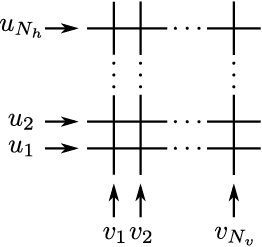
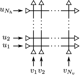
Once we fix all configuration arrows, i.e. white arrows, at the boundary we can calculate the partition function using the Boltzmann weights defined in (1) and (2). It is defined by
| (4) |
Depending on the internal states, i.e. white arrows at the edges of a vertex, the weight is given by or as introduced in (3). Summing over all possible state configurations in the interior of the lattice then yields the partition function. As an example let us consider the case given in Figure 1(b). In this case the partition function is particularly easy to calculate as there is only one configuration of internal arrows allowed at each vertex. This can be seen from (1) and (2). Starting from the lower left vertex in Figure 1(b) we see that the only allowed local configuration is the first vertex with weight in (1). As a consequence the same is true for the next vertex on the right. Now proceeding line by line from bottom to top we find that the sum in (4) is trivial and obtain
| (5) |
In general for an arbitrary lattice as the ones given in the beginning of this chapter we can associate an orientation and a spectral parameter to each line and calculate the partition function on that lattice after fixing a certain boundary configuration via the formula
| (6) |
Here the argument of the Boltzmann weight depends on the orientation and rapidities of the two crossing lines. For convenience we suppressed the dependence on the state variables.
2 Relation to R-matrix
The careful reader might have noticed that the Boltzmann weights of the six-vertex model (3) are related to the entries of the -invariant R-matrix introduced in (1) via
| (1) |
To relate the graphical notation used in the previous chapter to the one used in Section 1 we note that in Chapter 1 an orientation was introduced at each line of a vertex to distinguish left and right multiplication in each of the spaces on which the R-matrix acts non-trivially, compare (4). However, these black arrows on the lines introduced for this purpose should not be confused with the white arrows used to label the different states of the six-vertex model. The black arrows correspond to the black arrows in (1) and (2) and the white arrows translate into the row and column indices of the matrix (1) acting on the tensor product . If a white arrow points into the same direction as the arrow that denotes the orientation of the line we replace it by the state label . If it is pointing in the opposite direction we assign the state label . Thus, in this notation the vertex configurations of the six-vertex model in (1) and (2) are depicted as
| (2) |
| (3) |
Here, according to (1), all other vertex configurations are identical to zero. Furthermore, we would like to note at this point that the ice-rule translates into the charge conservation condition with which follows from the -invariance of the R-matrix. As a consequence the states assigned to the bottom and left edge have to reappear at the top and right of each vertex.
In general, we can think about the entries of an arbitrary -invariant R-matrix denoted by as Boltzmann weights. Here the indices and take the values , where denotes the dimension of the representation in space respectively. Graphically this is denoted as
| (4) |
compare (1). This notation has the advantage that the relation to our previous studies becomes more transparent. Whenever we talk about the components of the R-matrices, i.e. Boltzmann weights, we indicate the corresponding indices at the end of the lines as shown in (4). Here we have neglected the rapidities, they are assigned in the same way as in (4).
3 Partition functions and QISM
We are now in the position to study the partition function of the six-vertex model using the QISM. In particular, we can write the partition function in (4) for a given boundary configuration as a product of monodromies of length introduced in (1) with inhomogeneities and fundamental representation of in quantum and auxiliary space
| (1) |
Here the set of indices label the configuration at the boundary, compare Figure 1(a). In our notation and are associated to the external edges of the lattice to the left and bottom respectively. The external states at the right and top are labeled by and . For cylindrical boundary conditions in the horizontal direction we contract the indices and which yields the transfer matrix introduced in (4) or pictorially in (5)
| (2) |
The partition function defined on a cylinder as shown in Figure 1(a) for a given boundary configuration takes the form
| (3) |
This is the same transfer matrix as the one we have diagonalized using the Bethe ansatz in Chapter 1. Let us now consider the partition function on a toroidal topology as shown in Figure 2(b). It can be obtained from (3) by contracting the indices that now correspond to the edges in the vertical direction
| (4) |
The partition function is invariant under basis transformations. Hence it can be written in terms of eigenvalues of the transfer matrices
| (5) |
see e.g. [88, 89]. Here denotes the eigenvalue of the transfer matrix . Thus we obtained an expression for the partition function defined on a torus parametrized by Bethe roots satisfying the corresponding Bethe equations. Again, as discussed previously in Section 9, the issue of completeness of the Bethe equations arises in this context. Furthermore, we would like to note that our derivation of (5) heavily relied on the the quantum inverse scattering method which was not at hand in 1967 when Lieb presented his solution. His derivation is along the lines of Bethe’s original approach from 1931 presented in Section 10.
We end this section with the example shown in Figure 1(b) where some vertical lines are oriented in the opposite direction in order to prepare the reader for the discussion in Chapter 5. Let be the monododromy describing a horizontal layer with an opposite orientation at site . It takes the form
| (6) |
where denotes the transposition in the vertical space. The permutation operators ensure that the vertex is oriented properly and the transposition is necessary to write the partition function as a product of transfer matrices, compare (3). Using crossing symmetry this transfer matrix can be rewritten in the familiar form. In particular, this is discussed in the next sections.


4 Symmetries of the R-matrix
We would like to study some of the discrete symmetries of the R-matrix in (1). For this purpose we extend our analysis to the -invariant R-matrix in the fundamental representation as introduced in (1). It contains the same weights as the -invariant R-matrix but in total there are vertices. In components the only difference lies in the range of the indices. We have
| (1) |
with . From (1) we see that the Boltzmann weights are left invariant under the transformation :
| (2) |
This reflects the symmetry under transposition in both spaces and of the R-matrix. Furthermore, we also find that (1) is left invariant under substituting and therefore
| (3) |
Note that here the indices belonging to space on the left hand side of the equation are identified with the indices of space on the right hand side and vice versa. This identification of with is possible as we have the same representation in the spaces and . The symmetries discussed above can be encoded into the pictorial equivalence relation
| (4) |
5 The anti-fundamental representation
In the following we introduce the R-matrix with the fundamental representation in the first space and the anti-fundamental in the second. The generators of the anti-fundamental representation are of the form
| (1) |
The representation is labeled by which is denoted by in the following. It is straightforward to show that this choice indeed satisfies the algebra (4), see also next section. Let us again start with the case. In analogy to (1) we can write the R-matrix as
| (2) |
where we used the definition of the Lax operators in (5). For short we denote this R-matrix as , keeping in mind that
| (3) |
The entries of the R-matrix (2) are given by
| (4) |
As before we proceed to the corresponding -invariant R-matrix. Again, the only difference is the range of the indices and we find the general expression
| (5) |
for . Diagrammatically we denote this R-matrix as
| (6) |
where we introduced the white dot to distinguish it from the R-matrix introduced previously, cf. (4). The vertical line corresponds to the space in the anti-fundamental representation. This R-matrix has the same symmetries under the exchange of indices as the . Namely under the transformation we find
| (7) |
and moreover the transformation yields
| (8) |
Here we note that the dimension of the fundamental and anti-fundamental representation are the equal, thus the indices of space and take the same values which makes the identification in (8) possible. Diagrammatically we write these relations as
| (9) |
6 Crossing symmetry
The goal of this section is to relate the R-matrix with fundamental representation of in both spaces with the R-matrix whose second space is in the anti-fundamental representation. The relation can be motivated from the existence of the outer automorphism 11 1 Note that for the case the two representations are equivalent. of
| (1) |
Under the action of the automorphism the Dynkin labels transform as
| (2) |
compare also to the choice of the generators in (1). First, we allow a normalization of the R-matrix that we did not include up to now as it cannot be determined from the Yang-Baxter equation. However, in the following it plays an important role. Thus, we rewrite the R-matrices introduced previously as
| (3) |
and
| (4) |
with . From (1) and (5), where we expressed the R-matrices under study in terms of components, we find that the two R-matrices can be related via
| (5) |
This condition naturally imposes the relation among the normalizations of the R-matrices in (3) and (4)
| (6) |
Using the symmetries discussed previously we note that (5) can be rewritten as
| (7) |
Thus graphically this relation can be expressed as
| (8) |
which can be interpreted as a “rotation” of the vertex given in (4) by . Crossing relations like the one in (8) naturally appear in the study of integrable quantum field theories [90, 91]. We use this property to relate the partition function of the vertex model in Figure 1(b) to the commuting family of operators. Using the notation for denoting the R-matrix with the antifundamental representation in space , we find that the monodromy matrix discussed in (6) for can be rewritten as
| (9) |
which fits into the monodromies studied in the previous chapter and therefore can be diagonalized using the Bethe ansatz. This holds true generally for the extension to along the lines as discussed in this section.
Let us also consider the partition function on the torus defined in (4). As a consequence of (7) there exist two equivalent ways to write the partition function in terms of transfer matrices. In Section 2 we thought about the partition function as the trace of transfer matrices of length , however we can also think about it as the trace of transfer matrices of length . It yields a representation of the partition function
| (10) |
with the transfer matrices formed out of the R-matrices in (4)
| (11) |
Again, this prescription applies in the general framework of this section but it has an important implication for the case of where the outer automorphism discussed in (1) becomes an inner automorphism. Therefore, the anti-fundamental representation can be directly related to the fundamental. To be precise, for
| (12) |
we find that
| (13) |
with the similarity transformation containing the Levi-Civita symbol
| (14) |
See also [92], where this relation is discussed for the trigonometric case. For general such a relation does not exist as for the anti-fundamental and fundamental representation are not equivalent. After substituting (13) into (11) the similarity transformations in the auxiliary space cancel each other under the trace and we obtain
| (15) |
Having in mind the integrability condition (6) we conclude that
| (16) |
where we denoted the collective shift in the variables by . This so-called modular identity is an important step when studying the thermodynamic limit [93, 89].
7 Z-invariance
Now, we consider a slight generalization of the lattice presented in Figure 3(b). The new feature that appears is that the lines are allowed to intersect asymptotically. We assign rapidities and orientations to the lines as shown in Figure 1(a) such that all lines point from the bottom to the top. The major point we want to make here is that the lines can be moved freely as long as their endpoints do not intersect. This can change the form of the lattice but will not change the partition function. This is a consequence of the Yang-Baxter equation
| (1) |
which we studied in detail for certain R-matrices in the previous chapter, compare e.g. Figure 6. The property that the partition function (6) is invariant when the lattice is changed accordingly is usually referred to as -invariance, see [94] and in particular [95] for a detailed discussion 22 2 We thank Patrick Dorey for pointing out this reference.. As a consequence the partition function is completely determined by the boundary data which contains the external state labels and the enumeration of the lines. Thus, we do not have to care about the actual lattice configuration inside as shown in Figure 1(b) as long as we don’t allow self- nor double-crossings of the lines.


8 Unitarity
As a consequence of the Yang-Baxter relation (3) there naturally arises a symmetry among R-matrices. This symmetry relates the R-matrix to the one where spaces and are exchanged, namely . To obtain this relation we multiply the Yang-Baxter equation (3) from both sides with the inverse of and obtain
| (1) |
Exchanging the spaces and in (3) we observe that the inverse of satisfies the same Yang-Baxter equation as . Thus, assuming that the solution is unique, we conclude that they are proportional to each other
| (2) |
It is convenient to fix the normalization in such a way that (2) becomes an equality. This yields the unitarity relation
| (3) |
Graphically this equation is depicted in Figure 1.

It has a natural interpretation in terms of integrable field theory where we can think of two particles scattering and rescatter again, see eg. [42, 96].
1 An example
In this section we consider a general lattice as introduced in Figure 1(a) but allow for multiple intersections of the lines as shown in Figure 2. We concentrate on the -invariant R-matrices with fundamental and anti-fundamental representations in either of the two spaces as introduced in (3) and (4). Let us now consider the lattice presented in Figure 2. As shown in the figure we allow to associate different, i.e. fundamental and anti-fundamental, representations of to each line. In this sense it is more convenient to think about Figure 2 as a product of R-matrices instead of a lattice with Boltzmann weights. Also, as discussed below, the fact that the structure of the lattice can be changed according to the unitarity relation depicted in Figure 1 makes this interpretation more natural.

We already encountered two of the -invariant R-matrices that appear in our example, i.e.
| (4) |
as defined in (3) and (4) containing the normalizations and . In addition we introduce the two R-matrices
| (5) |
which can be obtained from the relation (2) and
| (6) |
that can be derived from the Yang-Baxter equation (3) rather quickly noting that intertwines two R-matrices and using (5). Furthermore, we fix a relative normalization such that
| (7) |
This equation without the shift in the spectral parameter is fulfilled trivially for the R-matrix as both spaces are in the same representation. The same holds true for . Pictorially, this relation can be written as in Figure 1 for .
Let us impose the unitarity condition in (3) to determine the normalization and introduced previously. In principle, there are four ways to assign the representations to the two lines in Figure 1: , , , . However, the unitarity conditions for and are equivalent. Furthermore, it follows from (6) that also the cases and yield the same relation. First, we consider the case where we have two fundamental representations. We impose
| (8) |
and obtain the condition
| (9) |
for the normalization . Following the same strategy for the case where we have one fundamental representation and one anti-fundamental
| (10) |
with the normalization , cf. (4) and (7), we obtain
| (11) |
The normalizations defined implicitly by (9) and (11) allow to disentangle the lines in Figure 2 according to Figure 1. We find that with this choice the lattice given in Figure 2 is equivalent to the one presented in Figure 1(a). In this sense we can generalize the notion of -invariance discussed in Section 7.
Last but not least, we would like to give an explicit solution that satisfies the unitarity conditions (9), (11) and additionally the crossing relation (8) of the -invariant R-matrices discussed here. It takes the form
| (12) |
This normalization is not unique as one can multiply it with arbitrary functions that satisfy
| (13) |
Here is the so-called CDD factor [97] which is of crucial importance in integrable field theories. In particular different CDD factors may yield different theories. As this will not be crucial in the following we do not elaborate further on this subject. Further details can be found in e.g. [98, 42, 96].
9 Crossing and unitarity for Lax operators
For later purposes we discuss the crossing and unitarity relation for the Lax operators introduced in (5) to construct the spin-chain monodromy (1). These R-matrices have the fundamental representation of in the auxiliary space and representation in the quantum space, cf. (2). As in Section 6 we allow for a normalization that cannot be obtained from the Yang-Baxter equation
| (1) |
To determine we follow the method introduced in Section 8 and determine the inverse of the Lax operator (1). For representations that satisfy the condition 33 3 See also Section 2 for further details on this type of representations.
| (2) |
with and the identity in the appropriate representation , one obtains
| (3) |
Using the proportionality relation (2) then yields the R-matrix . In addition we impose the relation
| (4) |
to fix the normalization, see Figure 1.

Now, imposing the unitarity condition as introduced in (3)
| (5) |
we obtain a difference equation for the normalization
| (6) |
cf. (9).
Next, we introduce using the algebra automorphism in (1). From (5) we find that it can be written as
| (7) |
Here we would like to stress that we employ the generators of representation to realize the R-matrix of the cojugate representation as discussed in (2). Following the same reasoning as before we determine through the inverse of and fix the normalization such that
| (8) |
where we used the condition on the representation introduced in (2). For the R-matrices and the unitarity relation reads
| (9) |
It yields the difference equation
| (10) |
for the normalization . Here we introduced the complex numbers and via
| (11) |
Their relation to and is given by
| (12) |
For the fundamental representation we find the values
| (13) |
Thus, from (6) and (10) we reproduce as special cases the difference equations derived earlier in (9) and (11).
In the end we present the crossing relation for Lax operators. This relation was discussed in Section 6 for the fundamental/anti-fundamental representation of . In general for an arbitrary representation with we obtain the crossing equation
| (14) |
and thus the relation between their normalizations
| (15) |
compare (6).
10 Three-vertices from R-matrices
In this section we introduce certain intertwiners that can be interpreted as three-vertices. We focus on a rather simple example and postpone a more general discussion to the next section and Chapter 5. Let us recall the R-matrix with the fundamental representation of in quantum and auxiliary space
| (1) |
Apart from the permutation point which, as we discussed in Chapter 1, is of crucial importance to obtain local charges in the framework of the quantum inverse scattering method there are two special points of the spectral parameter where the rank of the R-matrix is reduced. This can be seen if one rewrites the R-matrix in terms of projectors, see e.g. [99],
| (2) |
with . One immediately sees that these points are located at . We will be interested in the case where the R-matrix reduces to the projector on the symmetric representation in the tensor product decomposition of two fundamental representations
| (3) |
The projector can be factorized into the product of two rectangular matrices
| (4) |
which are related to each other by transposition. Here is an matrix that can explicitly be written as
| (5) |
Here we employed the notion of Young tableaux to denote the normalized basis vectors, see e.g. [100, 101]. As an example let us consider the case. For we find
| (6) |
From the tensor structure of in (5) we see that it provides a linear map
| (7) |
where is the dimension of the symmetric representation in (3). Thus, in the following we denote as three vertices
| (8) |
It follows that the R-matrix (2) at the special point can be written diagrammatically as
| (9) |
Both vertices and are invariant under permutation of the two spaces that are in the fundamental representation
| (10) |
and from the projection property of it follows that
| (11) |
which we denote graphically as
| (12) |
The three-vertices introduced in (8) will be studied on more general grounds in the next section and in particular in Chapter 5. At this point, we will also come back to the discussion of the special points of the R-matrix.
11 Bootstrap equation
It is interesting that the three-vertices introduced in the previous section satisfy a Yang-Baxter like equation. Namely, it holds that
| (1) |
In this case, the corresponding relation involving can be obtained by transposing (1) in all spaces. Furthermore, here transposition in space 1, which is suppressed in the notation above, relates the equation to one involving crossed Lax matrices, cf. (3) where this operation inverts the orientation of line 1. For a proof of these relations we refer the reader to Chapter 5. At this point we would like to stress that the so-called Bootstrap equation [102] above is not a consequence of the Yang-Baxter equation. As we will see in Chapter 5 the Yang-Baxter equation can be reconstructed from it in certain cases. We introduce it through the generic form
| (2) |
where is some projector from onto a subspace , cf. (5). In addition there is a constraint on the spectral parameters that depends on the representations under study. Pictorially, we denote the bootstrap equation as
| (3) |
In integrable field theories we think about two particles and that form a bound state .
The fusion procedure of R-matrices, see e.g. [63], can be understood in this framework. Multiplying the bootstrap equation (1) with from the left and subsequently using the relation in (11) we find an expression for Lax matrix with representation in terms of the two Lax matrices
| (4) |
Diagrammatically this relation can be depicted as
| (5) |
where the vertical space denotes the auxiliary space of the Lax operators. A nice feature of the bootstrap equation and the fusion procedure is that we can generate the crossing normalizations of the R-matrices. Following [63] we obtain the crossing normalization for Lax operators with symmetric representations from introduced in (12) for the case
| (6) |
It can be checked that this function indeed solves the constraints on the normalization for and as discussed in Section 9. For the example above we find that
| (7) |
here the terms and arise from the two Lax matrices in the fundamental representation, cf. (4).
Chapter 3 Yangian
In this chapter we discuss aspects of the Yangian. This infinite-dimensional Hopf algebra, named after C.N. Yang, was introduced by Drinfeld in 1985 [55, 56]. It naturally appears in the context of the Yang-Baxter equation and the quantum inverse scattering method. There are three different realizations of the Yangian, usually refered to as Drinfeld’s first realization, Drinfeld’s second realization and the RTT-realization. We are mainly interested in the RTT-realization which is closely tied to the RTT-relation (7). We discuss how the Yangian algebra arises in this framework and study certain automorphisms and anti-automorphisms. Furthermore, we introduce the quantum determinant which generates the center of the Yangian. We introduce the coproduct and discuss its action on the Yangian generators to motivate the relation between the RTT-realization and Drinfeld’s first realization that can be found in Appendix 9. Last but not least we discuss the Yangian generators of rational spin chains and exemplify the use of the coproduct and antipode.
Here we will closely follow the presentation in [103] and refer the reader to this reference for proofs and further studies. Other sources are [81, 104, 105, 82, 106, 107, 108].
1 Yang-Baxter algebra
We start our discussion with the Yang-Baxter equation (3) written in the form
| (1) |
Here is the R-matrix in the fundamental representation (1) acting on the spaces and . Furthermore, we assume that the remaining two R-matrices are matrices with operatorial entries
| (2) |
For later purposes we suppressed the indices indicating on which spaces the R-matrices act trivially and used the notation
| (3) |
where the identity indicates the trivial action on the space and , respectively. The Yang-Baxter equation (1) is a defining relation for the Yangian algebra [55]. Using our previous result (3) we eliminate the dependence on the spaces and and obtain the commutation relations
| (4) |
for the entries of the matrix introduced above. The formal Laurent expansion
| (5) |
with yields the generators of the Yangian . As mentioned previously, we will discuss certain degenerate solutions with that are relevant for the construction of Q-operators in Chapter 4. Using (4) and the geometric series expansion, we obtain a system of relations for the Yangian generators . They satisfy the Yangian algebra
| (6) |
By construction, these relations are equivalent to the RTT-relation (1).
Let us recall the Lax operator (5). This solution to the Yang-Baxter equation was constructed from the ansatz given in (2). As discussed any solution to the Yang-Baxter equation can be multiplied by a function. Thus dividing (2) by the spectral parameter we find that our ansatz is equivalent to the case where
| (7) |
In this case the commutation relations of the Yangian algebra (6) reduces to the commutation relations as discussed in Section 3. In the mathematical literature this representation is usually referred to as the evaluation homomorphism from the Yangian to the universal enveloping algebra of .
2 Automorphisms
We will now discuss certain operations on the monodromy
| (1) |
such that still satisfies the Yang-Baxter equation (1) and therefore leave (6) invariant. As discussed previously any solution of the Yang-Baxter equation can be multiplied by a scalar function and remains a solution. For
| (2) |
we find that the Yangian algebra (6) remains invariant. Thus the operation
| (3) |
is an algebra automorphism. Furthermore, we have the freedom of shifting the spectral parameter
| (4) |
by some complex number . This leaves the Yangian algebra (6) invariant as the R-matrix in (1) enjoys the difference property, namely it only depends on the difference of the spectral parameters . Additionally, for any invertible matrices which act trivially in the quantum space one has the automorphism
| (5) |
This follows from the property
| (6) |
3 Anti-automorphism and antipode
The anti-automorphisms map the solutions of the Yang-Baxter equation (1) to solutions of the equation
| (1) |
The crucial difference in this equation compared to (1) is the order of multiplication in the quantum space. It is rather straightforward to see that the inversion
| (2) |
satisfies (1). We discussed a similar phenomenon in Chapter 2, see (1). The mapping in (2) is usually referred to as the antipode. Additionally, we have the transposition in the auxiliary space
| (3) |
We can show that (1) is satisfied by transposing (1) in the two auxiliary spaces and by using the symmetry of the R-matrix . Furthermore, one has the reflection
| (4) |
which follows from the relation
| (5) |
cf. (9) and the automorphism (3). In particular, the fact that the composition of two anti-automorphisms yields an automorphism can be used to fix a certain normalization for . This was discussed in detail for the Lax operators in Section 9. For completeness we give the analogues of the defining relations of the Yangian algebra (6)
| (6) |
4 Quantum determinant and
As we have seen in Section 10 the R-matrix becomes a projector on at the special points on the symmetric and antisymmetric representation in the tensor product decomposition (3). Previously we were interested in the case where the R-matrix becomes a symmetrizer. The definition of quantum determinant incorporates the other special point where the R-matrix reduces to the anti-symmetrizer
| (1) |
This property together with the RTT-relation (1), which simplifies for the choice of the spectral parameters as in (1) (compare (11) and (12)), motivates the definition of the quantum determinant. Here we only present the main properties of the quantum determinant and refer the reader to [103, 82, 81, 106] for their derivations. From the form of the R-matrix and the RTT-relation (1) it follows that the quantum determinant is given by
| (2) |
Here the sum goes over all permutations of . The quantum determinant of belongs to the center of
| (3) |
Expanding the quantum determinant in inverse powers of the spectral parameter yields
| (4) |
As a consequence of (3), the elements commute among themselves and with all Yangian generators. They generate the center of . In analogy to ordinary Lie groups one defines to be isomorphic to the quotient
| (5) |
5 Comultiplication
The product in the auxiliary space of any two solutions of the RTT-relation (1) yields another solution of the RTT-relation. This can be shown directly using the RTT-relation (1) or diagrammatically using the train argument presented in (8). We relied on this important property of the Yang-Baxter equation when constructing the commuting family of operators in Chapter 1. In the mathematical literature this structure is usually referred to as the coproduct. It should not be confused with the multiplication in the quantum space that appears in the RTT-relation. In the RTT-realization of the Yangian the coproduct is simply given by matrix multiplication in the auxiliary space and the tensor product in the quantum space
| (1) |
As mentioned above, the coproduct satisfies the compatibility condition
| (2) |
Furthermore, it can be shown that the quantum determinant introduced in the previous section is comultiplicative
| (3) |
The coproduct, together with the antipode introduced in (2) and the counit
| (4) |
are characteristic structures of a Hopf algebra. We will not further elaborate on the Hopf algebra structure of the Yangian as it is not necessarily needed to follow the subsequent presentation and refer the reader to the literature. For a mathematical approach see e.g. [105, 109] as well as the PhD thesis [110] and for a physicist’s presentation see e.g. [81, 104].
We would like to make a few more comments at this point that we find helpful to understand the relation of the RTT-realization to Drinfeld’s first realization of the Yangian that is discussed in Appendix 9. In order to do so, we present the action of the coproduct on the Yangian generators introduced in (5) which can be obtained from the expansion of (1) using (5). In general it can be written as
| (5) |
Hence, we see that for we obtain
| (6) |
which is familiar from the representation theory of Lie algebras and quantum mechanics. For higher orders we get a deformation of this term as for example for
| (7) |
The action of the antipode on the first two Yangian generators is given by
| (8) |
and
| (9) |
Using the ordinary multiplication (multiplication in the quantum space) of the Hopf algebra that we did not introduce explicitly we can verify (8) and (9). Knowing the Yangian algebra (6) and the action of the coproduct and antipode on the Yangian generators we can in principle forget about the auxiliary space and the RTT-relation. However, naively we still have to deal with infinitely many generators. The beauty of Drinfeld’s first realization is that the Yangian is characterized by the first two levels and an additional algebraic constraint called Serre relations. Solving these equations and imposing the structure introduced previously one can reformulate the Yangian without the need of a Yang-Baxter equation. The explicit connection between the two realizations of the Yangian is presented in great detail for the case of in [81]. We are not aware of a reference where this has been worked out for . In Chapter 5 we will discuss some advantages and disadvantages of Drinfeld’s first realization and the RTT-realization.
6 Yangian and spin chains
Let us recall the spin chain monodromy introduced in (1) with all inhomogeneities set to zero. As shown graphically in (8), this monodromy satisfies the RTT-relation (1) and therefore yields a realization of the Yangian algebra (6). Defining
| (1) |
we can extract the form of the Yangian generators from the expansion in terms of the spectral parameter
| (2) |
cf. (5). We have already seen in Section 5 that the term proportional to is given by
| (3) |
The term proportional to is bi-local, i.e. it acts on non-adjacent sites of the quantum space and takes the form
| (4) |
To end this chapter, we present the action of the coproduct and the antipode for spin chains. The coproduct in (5) adds sites to the spin chain. For convenience we introduce the notation
| (5) |
It is rather easy to verify that
| (6) |
For the second level we find
| (7) |
which is compatible with (4).
The action of the antipode on the first and second level Yangian generators can be deduced from the inverse of the monodromy which can be constructed from the inverse Lax operators introduced in Section 9. Here we would like to remind the reader that we focussed on a certain class of representations satisfying the relation (2). The inverse of the monodromy can then be written as
| (8) |
Expanding the inverse monodromy above yields the action of the antipode
| (9) |
and
| (10) |
These relations are in agreement with the general formulas given in (8) and (9) and naturally generalize to inhomogeneous spin chains as the ones studied in Chapter 5. In particular, for a certain normalization of the monodromy matrix the Yangian generators for the inhomogeneous spin chain can simply be obtained by shifting the generators at each site .
Chapter 4 Q-operators
In this chapter we present a systematic approach to the construction of Baxter Q-operators for rational homogeneous spin chains. This program is motivated by the desire to gain a deeper understanding of the integrable structure of the free/planar AdS/CFT system, where spin chains appear in the weak coupling limit [18]. Although the R-operators provided in the Appendix 13 can be used to construct the Q-operators relevant for the full one loop spin chain of AdS/CFT there has not been any direct application of the method presented in the following, yet. However, the current techniques used to determine anomalous dimensions are based on the imposed analytic structure of all loop Q-functions, see [24] and references therein. Therefore, one may hope that it is possible to construct Q-operators at any value of the ’t Hooft coupling leading to the all loop Q-functions and containing the full information about the eigenspace.
We start the chapter with a review of the Q-operator construction for spin chains carried out in [27] and discuss how the functional relations among the Q-operators and the Bethe equations can be derived. Generalizing the construction to spin chains, we develop a new approach to Baxter Q-operators by relating them to the theory of Yangians, which are the simplest examples for quantum groups. A historic overview of the subject with references to earlier works can be found in Section 5 of [27]. Furthermore, a significant part of the PhD thesis [111] is dedicated to the Q-operator construction for invariant spin chains, cf. Section 2. In particular, it contains a careful analysis of the R-operators used in the Q-operator construction which we do not discuss here in its full extent. The method to obtain local charges from the Q-operators presented in Section 3 as well as the Lax operators (7) are not contained in [111].
Following the construction of Bazhanov, Lukyanov and Zamolodchikov [30, 31, 32], we study certain degenerate solutions of the Yang-Baxter equation connected with harmonic oscillator algebras. These infinite-state solutions of the Yang-Baxter equation serve as elementary, “partonic” building blocks for other solutions via the standard fusion procedure. After a reviewing the Q-operator construction for compact spin chains with the fundamental representation at each site of the quantum space we consider compact spin chains and derive the full hierarchy of operatorial functional equations for all related commuting transfer matrices and Q-operators 11 1 See also [112, 113, 114] for independent approaches.. This leads to a systematic and transparent solution of these chains, where the nested Bethe equations are derived in an entirely algebraic fashion, without any reference to the traditional Bethe ansatz techniques. Furthermore, we discuss the Q-operator construction for spin chains with more general representations of at each site of the quantum space and derive the corresponding Bethe equations. In the last part of this Chapter, we discuss how the shift operator and the Hamiltonian enter the hierarchy of Baxter Q-operators in the example of homogeneous spin-chains. We find that a reduced set of Q-operators can be used to obtain local charges. The mechanism relies on projection properties of the corresponding R-operators on a highest/lowest weight state of the quantum space. It is intimately related to the ordering of the oscillators in the auxiliary space. We introduce a diagrammatic language that makes these properties manifest. This approach circumvents the paradigm of constructing the transfer matrix with equal representations in quantum and auxiliary space and underlines the strength of the Q-operator construction.
We would like to stress that in Chapter 1 and 5 we build monodromies from R-matrices where the first space was taken to be the auxiliary space. This is a matter of conventions and one can equally well built them from R-matrices where the second space is the auxiliary space. In Section 9 we introduced the symmetry relation (4) that relates the two monodromies above if the auxiliary space is in the fundamental representation and the quantum space satisfies the relation (2). In this case we find
| (1) |
where for convenience all representations at the sites were taken to be equal. Thus, the two transfer matrices are related by a shift in the spectral parameter and therefore belong to the same family of commuting operators. In the following we focus on type transfer matrices following the conventions used in [27, 26, 28, 29, 34].
1 Q-operators in a nutshell
In the following we focus on the Q-operator construction for -invariant homogeneous spin chains with fundamental representation at each site of the quantum space. Following [26, 27], see also [18], we employ certain solutions of the Yang-Baxter equation (1) to derive the Baxter equation and the Bethe equations without referring to a vacuum nor making an ansatz for the eigenstates, cf. Section (1).
In Section 3, we derived the Lax operators from the Yang-Baxter equation making the ansatz (2). Later on we saw that this solution yields a realization of the Yangian, cf. Chapter 3. In the following we concentrate on the partonic Lax operators
| (1) |
with
| (2) |
As shown in Section 1, they satisfy the Yang-Baxter equation
| (3) |
cf. (1), where the third space has been realized using the harmonic oscillator algebra (2). In contrast to the Lax operators introduced previously, the term proportional to the spectral parameter is not the identity matrix.
It is easy to show that the product of the two solutions (1) is related to the ordinary Lax operator as introduced in Section 3. For this purpose we multiply the two partonic Lax operators (1) in the fundamental space and take the tensor product in the oscillator space. We obtain the factorization formula
| (4) |
where the additional labels carried by indicate the two copies of the oscillators and and
| (5) |
The -generators on the left-hand side of (5) are realized by the oscillators in Holstein-Primakoff form [115] as
| (6) | ||||||
satisfying the commutation relations as given in (4). We denote the Lax operator using a calligraphic letter to stress that the generators are realized using oscillators as above. Furthermore, we defined the complex variables
| (7) |
as well as the similarity transformation acting solely on the oscillators
| (8) |
Following the vertex notation introduced in Chapter 2, we can write the factorization formula (4) using the notation and as shown in Figure 1.

Using the Holstein-Primakoff realization of the generators (6), we fix the highest weight state to be the Fock vacuum
| (9) |
where we suppressed the index carried by the oscillators. The action of the generators (6) on the highest weight state is then given by
| (10) |
and we label the representation as . Furthermore, we note that for a given positive integer a representation with is finite-dimensional and the lowest weight state annihilated by is of the form , cf. Figure 3.
The factorization formula (4) is of prior importance to derive the functional relations among the Q-operators and the transfer matrices with fundamental representations in the quantum space and various representations of in the auxiliary space. A similar formula where the order of the partonic Lax operators is reversed can be found in [26]. Like the transfer matrices in Chapter 1, the Q-operators are constructed as traces over monodromies built out of the partonic Lax operators (1). They are defined as
| (11) |
with the trace explicitly given by
| (12) |
and the normalization
| (13) |
Here the auxiliary space is the Fock space generated by the oscillators , while the quantum space is given by the -fold tensor product of . Hence, (11) is a matrix. Naively, the trace over the infinite-dimensional Fock space diverges. Thus, we introduce a twist containing the complex parameter in analogy to Section 9, see also Section 3 for further details.
Using the factorization formula (4), one can show that the Q-operators defined in (11) are related to the transfer matrix 22 2 Note that we choose the auxiliary space to be the second space of the Lax operators. To obtain a monodromy whose auxiliary space is constructed from the first space of the Lax operators via the fusion procedure the degenerate solutions presented in Appendix 12 have to be employed.
| (14) |
via
| (15) |
Here we used the cyclicity of the trace and the relation
| (16) |
Diagrammatically it is easy to see that the similarity transformations cancel each other, see Figure 2.

However, when taking the trace over the complete Fock space, cf. (14), also states with contribute. These have to be subtracted by hand. As indicated in Figure 3, the superfluous states are given by the module with highest weight representation , i.e. the module defined through
| (17) |
see also [50]. The transfer matrix for finite-dimensional representations in terms of the transfer matrices defined in (14) then reads
| (18) |
As a consequence of the factorization formula (4) and the resulting relation (15), we obtain the transfer matrix in terms of the Q-operators
| (19) |
with .

The relation above is the main result of this section. It can be shown that the operators defined in this section commute with each other
| (20) |
Following the logic presented in Section 5, the first relation follows from the Yang-Baxter equation (3), the second and third one are more difficult to prove. We refer the reader to the discussion of the appropriate Yang-Baxter relations in [111]. To derive the Baxter equation, cf. (19), we evaluate (19) for the fundamental representation and for the trivial representation . Combining the two resulting relations we obtain the Baxter equation
| (21) |
Here we introduced the notation and . By construction the eigenvalues of the operators are polynomials of the form
| (22) |
with . Note, that we did not prove that is indeed diagonalizable. In order to do so, one should derive the appropriate Yang-Baxter relation to show that is a normal operator, i.e. it commutes with its transpose, compare Section 5. Following the argumentation in Chapter 1, we obtain the Bethe equations
| (23) |
from the Baxter equation (21). Noting that by construction is diagonal with eigenvalues 33 3 In this chapter we use the letter to denote the eigenvalues of the transfer matrix instead of . given by and using the explicit form of the Q-functions we find
| (24) |
The Bethe equations can also be derived directly from the functional relations (19) for , see Section 5.
To end this section let us connect our results to Chapter 1. Noting that
| (25) |
cf. Section 8, we obtain a slightly modified energy formula from the logarithmic derivative of the diagonal form of (21)
| (26) |
while the form of the Hamiltonian (10) coincides. This more symmetric form of the energy formula and the Bethe equations (24) with can be recast into the form introduced in (26) and (18) with vanishing inhomogeneities by shifting the Bethe roots
| (27) |
This naturally also yields a redefinition of the Q-functions which are polynomials with zeros located at the Bethe roots
| (28) |
such that we recover the Baxter equation (19) from (21). In Chapter 1, we only introduced one Q-function. The reason for this is that we fixed the reference state to be the -fold tensor product of highest weight states, cf. (4), and used the operators to create the eigenstates (7). However, we could have chosen the reference state to be the -fold tensor product of lowest weight states and create the Bethe vectors with the operator , cf. (1). This symmetry is reflected by the existence of the two Q-operators/functions, see also Section 4 and Section 5. Furthermore, later on we will discuss how the Hamiltonian can be obtained from the Q-operators. In particular, for the fundamental representation in the quantum space it is obtained in Appendix 14.C.
2 More on Q-operators
In the previous section we reviewed the construction of Q-operators for -invariant spin chains with a twist. In this section we generalize this construction for -invariant spin chains where the twist again plays an important role. We classify a set of degenerate solutions of the Yang-Baxter equation which constitutes the main ingredients to construct the full hierarchy of Q-operators for -invariant spin chains. We start with the construction of Q-operators with the fundamental representation at each site of the quantum space. A generalized factorization formula, cf. (4) and (15), allows us to construct the hierarchy of Q-operators and derive their functional relations. The Bethe equations follow from this construction. In Section 6 we present the R-operators that are the building blocks of Q-operators with arbitrary representations of at each site of the quantum space and derive the corresponding Bethe equations.
1 Representations of Yangians
The spin chain Hamiltonian (10) with twisted boundary conditions commutes with a large commuting family of operators and . In the following we explicitly construct these operators via traces of certain monodromy matrices associated with infinite-dimensional representations of the harmonic oscillator algebra. To do this we need to find appropriate solutions of the Yang-Baxter equation
| (1) |
where is an matrix,
| (2) |
acting in the direct product of two -dimensional spaces , cf. (1).
We will now show that there exist further first order operators, different from the Lax operators (5) and present their complete classification. For the case of these operators were introduced in (1). To begin, let us recall a symmetry of the Yang-Baxter equation (1). From the Yangian algebra (6) it follows that the elements are central, i.e. they commute among themselves and with all for . Therefore, we may regard as a numerical matrix. Applying the automorphism (5), this matrix can always be brought to a diagonal form
| (3) |
where is an integer . The number coincides with the rank of the matrix . Evidently, if , the leading term in the series expansion (5) is the unit matrix. This case is well studied in the existing representation theory, see e.g. [103]. In fact, the assumption that the series (5) starts with the unit matrix is usually included into the definition of the Yangian. Here we will not make this assumption, and consider the more general case with arbitrary .
Let us concentrate on the simple case when the series (5) truncates after the second term, i.e. assume that all for . It is convenient to write the only remaining non-trivial coefficient as a block matrix
| (4) |
where and are operator-valued matrices of dimensions , , and , respectively. We furthermore assume that all undotted indices run over the values , whereas their dotted counterparts take the values :
| (5) |
Substituting (3) and (4) into (6), one realizes that the elements are central, i.e. they commute among themselves and with all other elements of . The other commutation relations read
| (6) |
Using the remaining freedom of making the transformations (5), which do not affect the form of in (3), one can bring the matrix to a diagonal form with zeros and ones on the diagonal, in analogy to (3). Here we are only interested in highest weight representations of the algebra (6). These representations admit a definition of the trace, as required for the construction of transfer matrices in Section 3 below. For this reason we only consider the non-degenerate case 44 4 It appears that for the algebra (6) does not admit a definition for a suitable trace as needed for the construction of transfer matrices commuting with the Hamiltonian (10)., , where the diagonal form of coincides with the unit matrix
| (7) |
The resulting algebra (6) can be realized as a direct product of the algebra with copies of the harmonic oscillator algebra:
| (8) |
Therefore, we introduce independent oscillator pairs , where and , satisfying the relations
| (9) |
Furthermore, let , denote the generators of the algebra defined by (4), where is replaced by . The generators commute with all oscillators in (9). The connection of the algebra (6) with the product (8) is established by the following relations
| (10) |
where the hat in the notation denotes the transposition of the indices and ,
| (11) |
The corresponding L-operator can be written as a block matrix
| (12) |
where the rows are labeled by the indices or and the columns by or , in similarity to (4). Note that the matrix of the generators of , which enters the upper left block, is transposed, i.e. the -th row and -th column in this block contains the element .
The matrix (12) contains the parameter only in its first diagonal elements. By simultaneous permutations of rows and columns in (12) one can move these -containing elements to arbitrary positions on the diagonal, labeled by a set of integers . We shall denote the L-operator obtained in this way by . Within this convention the operator (12) corresponds to the set , as indicated by the subscript in the left hand side of this equation. Furthermore, employing the notation of Chapter 1 we note that the first space of the operator is in the fundamental representation .
The “partonic” L-operator
| (13) |
with
| (14) |
is a particular case of (12) with , while the standard Lax operator (5) corresponds to . For , these solutions were studied in e.g. [116, 117, 118, 119]. See also [120, 121] for more recent developments. For these solutions can be obtained in the rational limit of trigonometric solutions obtained in [60].
The L-operator in (12) provides an evaluation homomorphism of the infinite-dimensional Yangian algebra (6) into the finite-dimensional algebra (8),
| (15) |
This means that for any representation of this finite-dimensional algebra the equation (12) automatically defines a representation of the Yangian and a matrix solution of the Yang-Baxter equation (1). Conversely, any first order matrix L-operator with a rank leading term and a non-degenerate matrix in (4) is, up to a transformation (5), equivalent to the canonical L-operator (12) with some particular representation of the algebra (8). It is worth noting that the transformation (5)
| (16) |
where is a block diagonal matrix containing the matrix and the matrix on the diagonal, leaves the form of (12) unchanged.
2 Fusion and factorization of L-operators
An essential part of our analysis in the following is based on some remarkable decomposition properties of the product of two L-operators of the form (12). The coproduct of the Yangian
| (17) |
is generated by the matrix product of two L-operators corresponding to two different copies of appearing on the right-hand side of (17), cf. Section 5.
Our main observation is related to the coproduct of two operators and , defined by (12) for two non-intersecting sets ,
| (18) |
where the quantities denote arbitrary constants. Let the sets and contain and elements, respectively. The product (18) is of the first order in the variable , and that the matrix rank of the term linear in in (18) is equal to . The meaning of the comultiplication is that the matrix product of two L-operators, each of which satisfies by itself the Yang-Baxter equation (1), solves this equation as well, see (2). All solutions which possess the above properties were classified in the previous section. Therefore, by using a transformation of type (6), the right-hand side of (18) can be brought to a particular case of the canonical form (12) with . It turns out, however, that the expressions for the matrix elements of the resulting L-operator are rather complicated and their explicit connection to those of (12) is far from obvious, even though these elements satisfy the same commutation relations. In order to make this connection more transparent we apply a suitable operatorial similarity transformation to each matrix element such that it rearranges the basis of the oscillator algebras contained in , cf. (8). Furthermore, the formula (18) contains two constants and . Only their difference is an essential parameter, whereas the sum may be absorbed into the spectral parameter . Therefore, without loss of generality, one can set
| (19) |
where is arbitrary. This particular parametrization is chosen to simplify the subsequent formulas.
Proceeding as described above, one obtains,
| (20) |
where is a -independent matrix, whose elements commute among themselves and with all elements of . It should be stressed that the resulting L-operator is only a special case of (12), since it is connected to some specific realization of the algebra in terms of the direct product of the two algebras as defined in (8). Note that the right-hand side of (20) is a particular case of the transformation (5) with and . The explicit expressions for the matrices appearing in (20) are presented below.
By permuting rows and columns any two non-intersecting sets and can be reduced to the case when and . So it is suffficient to consider this case only. We introduce three types of indices
| (21) |
It is convenient to rewrite (12) as a block matrix
| (22) |
where and the size of the diagonal blocks is equal to , and , respectively. As before, the superscript “” indicates that the corresponding operators belong to the “first” algebra in the comultiplication (17), which in the considered case is realized by the algebra defined in (8). Similarly, one can write as
| (23) |
where and the superscript “” labels operators from the “second” algebra, which is the algebra . By construction, all operators labeled by the superscript “” commute with those labeled by the superscript “”. Recall also that the algebra (8) has a direct product structure, so the generators and commute with all oscillator operators.
With the notation introduced above the similarity transformation in (20) has the form
| (24) |
where
| (25) |
and
| (26) |
The matrix has the form
| (27) |
The similarity transform serves to expose the fact that the matrix entries of commute with the entries of . The similarity transform brings to the form (12).
Finally, we want to write the operator in (20) in the form (12) with . To do this we need to make the following identifications for the generators in the upper diagonal block of (12)
| (28) | |||||
where we have used the conventions (21) for numerating the indices.
Furthermore, let the indices run over the values and over the values . Introduce operators
| (29) |
Then the L-operator from (20) can be written as
| (30) |
which has the required form as in (12).
The formulas in (28) give a homomorphism of the algebra into the direct product
| (31) |
which for has only infinite-dimensional representations (similar representations appeared in [124]). An important feature of this map is that if one choses highest weight representations for both algebras and then (28) defines a highest weight representation of . The highest weight conditions (3) are satisfied on the product of the corresponding highest weight vectors and the standard Fock vacuum for all oscillator algebras appearing in (28). The -weight of the resulting representation is obtained from (28)
| (32) |
where is an arbitrary parameter, cf. (20).
The L-operators in the first product in (20) have the superscripts and , which indicate that they belong to different algebras (8) with and , respectively. By the same reason it is useful to rewrite the RHS of (20) supplying similar superscripts
| (33) |
where the superscript indicates the algebra (31) and the superscript indicates the product of oscillator algebras . Note that the matrix could be considered as a -independent L-operator, also satisfying the Yang-Baxter equation (1). In this sense (33) also describes the comultiplication of two representations of the Yangian.
Consider now some particular consequences of formula (20). Using it iteratively with and taking into account (32) one can obtain an arbitrary product of the elementary L-operators (13). Let be an ordered integer set, , and a specialization of the L-operator (12) to the infinite-dimensional highest weight representation of the algebra
| (34) |
Define also the shifted weights, cf. (57),
| (35) |
Then it follows from (20) that
| (36) |
where the matrices and are products of the expressions of the type (24) and (27) arising from the repeated use of the formula (20). In the particular case the last formula provides the factorization for the Lax operator (5),
| (37) |
evaluated for the infinite-dimensional highest weight representation in the auxiliary space,
| (38) |
cf. (28).
3 Construction of the Q-operators
The purpose of this section is to define the operators and . They have to commute with the Hamiltonian (10) of the twisted compact -spin chain of length . These operators act on the quantum space which is an -fold tensor product of the fundamental representations of the algebra ,
| (39) |
cf. Chapter 1. As before, solutions of the Yang-Baxter equation (1) are considered to be matrices, acting in the quantum space of a single spin. Their matrix elements are operators in some representation space of the Yangian algebra (6). This representation space will be called here the auxiliary space. For each solution of (1) one can define a transfer matrix,
| (40) |
where the tensor product is taken with respect to the quantum spaces , while the operator product and the trace is taken with respect to the auxiliary space . The quantity is a “boundary twist” operator acting only in auxiliary space, i.e. it acts trivially in the quantum space. This boundary operator is completely determined by the requirement of commutativity of the transfer matrix (40) with the Hamiltonian (10) and its generating transfer matrix, cf. (10). Following the same logic as in Section 9 we obtain the condition
| (41) |
It is convenient to parametrize the diagonal twist as
| (42) |
using the fields which enter in (41) only through their differences with
| (43) |
Solving (41) for the general L-operator (12) with an arbitrary set one obtains
| (44) |
which reduces for the fundamental representation and to (42).
In the following we will use some important properties of the trace over the Fock representations of the oscillator algebra
| (45) |
This algebra has two Fock representations,
| (46) |
and
| (47) |
spanned on the vectors , . These representations can be obtained from each other via a simple automorphism of (45) also refered to as particle-hole transformation
| (48) |
Let be an arbitrary polynomial of the operators and . Below it will be convenient to use a normalized trace over the representations ,
| (49) |
where is either or , and denotes the standard trace, cf. (12). An important feature of the normalized trace (49) is that it is completely determined by the commutation relations (45) and the cyclic property of the trace. It is therefore independent of a particular choice of representation as long as the traces in the RHS of (49) converge. Alternatively, one can reproduce the same result by using explicit expressions for the matrix elements of the oscillator operators in (49). Then the trace over converges when and the trace over when . Both ways of calculation lead to the same analytic expression for the normalized trace. Thus it is not necessary to specify which of the two representations is used.
We are now in the position to define various transfer matrices all commuting with the Hamiltonian (10). Consider the most general L-operator (12) with an arbitrary set , where . Recall that the matrix elements of (12) belong to the direct product (8) of the algebra and of oscillator algebras. Choose a finite-dimensional representation with the highest weight for the -factor of this product. Then substituting (12) and (44) into (40) one can define rather general transfer matrices
| (50) |
where is the corresponding monodromy matrix,
| (51) |
Here denotes the normalized trace (49) for all involved oscillator algebras 55 5 Note that all possible expressions under the trace in (50) for each oscillator algebra are exactly as in the LHS of (49) for some polynomial and some value of . Thus the definition (49) is sufficient to calculate all oscillator traces in (50)., while denotes the standard trace over the representation of . The exponential scalar factor in front of the trace is introduced for later convenience.
Similarly, one can define a related quantity where the -trace is taken over an infinite-dimensional highest weight representation ,
| (52) |
while the rest of the expression remains the same as in (50). Note that in the case of (50) the weights satisfy the conditions (5). In contradistinction, in (52) these weights are arbitrary.
In the limiting case , the general L-operator (12) simplifies to (5), while, as discussed above, the twist (44) simplifies to
| (53) |
In this case the definition (50) reduces to that for the standard T-operator
| (54) |
associated with the finite-dimensional representation of the algebra in the auxiliary space. Here denotes the Lax operator (5). However, we like to stress again that opposite to the definitions in Chaper 1, the spaces in the fundamental representation yield the quantum space and the auxiliary space is labeled by the representation label , cf. (1). Likewise, the formula (52) reduces to the T-operator
| (55) |
associated with the infinite-dimensional representation . The above two T-operators are connected due the Bernstein Gel’fand Gel’fand (BGG) resolution of the finite dimensional modules [125]. The BGG result allows one to express finite-dimensional highest weight modules in terms of an alternating sum of infinite-dimensional highest weight modules. This implies that the T-operator (54) for a finite-dimensional module can be written in terms of (55) as
| (56) |
where is a constant -component vector
| (57) |
The summation in (56) is taken over all permutations of elements, , and is the parity of the permutation . The relation (56) and its connection to the BGG resolution were first obtained in [126] in the context of , while the case was previously considered in [31, 32], see also Section 1.
Another limiting case of (50) corresponds to the representation turning into the trivial one-dimensional representation of with weight . As we shall see below the resulting operators
| (59) |
are actually the Q-operators, whose eigenvalues appear in the nested Bethe ansatz equations. Let us enumerate these Q-operators. It is convenient to start formally from the exceptional case , corresponding to an empty set . By definition we set
| (60) |
For the next level there are obviously sets consisting of just one element , . The general L-operator (12) in this case takes the simple form (13) and the twist operator (44) simplifies to
| (61) |
In this way one obtains from (50)
| (62) |
where , given by (13) and
| (63) |
More generally, for the level there are increasing integer sets , which numerate the Q-operators (59). For the highest level the definitions (59) and (50) immediately lead to the result
| (64) |
where is the length of the chain. Altogether there are different Q-operators including (60) and (64). As discussed in the next section, they can conveniently be associated with nodes of a hyercubical Hasse diagram.
The Q-operators form in conjunction with all T- and X-operators a commuting family and therefore can be simultaneously diagonalized. One sees that their eigenvalues have to be of the form
| (65) |
where, for each eigenstate, the numbers are the conserved occupation numbers,
| (66) |
cf. Section 2.
We would like to stress, that in general the operators , defined in (50), involve the trace over a representation of the Lie algebra and the trace over a number of Fock representations of the oscillator algebra, whereas the T-operators involve only the Lie algebra trace and the Q-operator only the oscillator traces. This is why we denoted the hybrid operators (50) by a distinct symbol .
4 Functional relations
The results of Section 2 imply various functional relations for the Q-operators. To derive them we need to use some additional properties of the twist operators (44) which are not immediately obvious from their definition (41). Let and be the operators (44), corresponding to and from the LHS of (20). By explicit calculation one can check that the product of these operators commutes with the similarity transformation defined in (24),
| (67) |
Moreover, this product can be rewritten in the form
| (68) |
where and are the twist operators obtained from (41) for the operator and the -independent L-operator from the RHS of (20). Again the relation (68) is verified by direct calculation, where one needs to take into account the explicit form of (27), (28), (29) and (30).
Next, define a scalar factor, cf. (19),
| (69) |
which depends on the set and the fields . Combining (20) with the definition (52) and taking into account (67) and (68) one obtains
| (70) |
There are two non-trivial steps in the derivation of the last formula which are explained in the following. First, the simple transfer matrix
| (71) |
that arises in the calculations is equal to the identity operator. Second, the scalar factors in (70) arise due to the difference in the definition of the trace over the oscillator algebras (normalized trace (49)) and over the representation of (standard trace). From (31) it is clear that oscillator pairs have to be “redistributed” to support the Holstein-Primakoff realization of the infinite-dimensional representation of the algebra .
A particular simple case of (70) arises when and ,
| (72) |
where by the definition (62) one has . Iterating the last formula one obtains
| (73) |
where the notation here is the same as in (35) and (36). Next, applying (58) one gets
| (74) |
and setting one finally arrives at
| (75) |
Note also that in the particular case the formula (74) leads to the determinant expression [31, 127, 32, 126, 128] for transfer matrix (54),
| (76) |
As previously mentioned the different operators can be assigned to the nodes of a hypercubic Hasse diagram. We will now show that four Q-operators belonging to the same quadrilateral as shown in Figure 2 satisfy a remarkably simple functional equation, which can be identified with the famous Hirota equation from the theory of classical discrete evolution equation, cf. (4). Define a matrix
| (77) |
where is an increasing sequence of integers which contains the subsequence with and .

Let us now use the Desnanot-Jacobi determinant identity, see Figure 1, for the matrix (77). Applying (75) for the subdeterminants one obtains the following operatorial functional relation 66 6 More general relations involving operators (74) can be obtained in the same way by replacing the arguments of the Q-operators in (77) with arbitrary constants , .
| (78) |
where is given by (69). Since all Q-operators commute with each other the same relation (78) holds also for the corresponding eigenvalues. In the next section, we use this to derive the Bethe equations and the energy formula. Furthermore, the quadratic functional relations (78) possess an interesting graphical interpretation, cf. Figure 2. The full set of functional equations is nicely depicted in so-called Hasse diagrams, cf. [33] and references therein. The Hasse diagram corresponding to the algebra forms an -dimensional ordered hypercube. Hasse diagrams for are presented in the Figure 3(a) and Figure 3(b), respectively. To read off the functional relations it is enough to take any 4-cycle in these diagrams, using the equivalence depicted in Figure 2.
Every path in the Hasse diagram which leads from to defines a system of equivalent but distinct nested Bethe equations. To find each such system, it is enough to take all Q-operators on a given path and write one relation for any three subsequent functions on the path. Such relation can be written for every three subsequent Q-operators because there always exists a unique 4-cycle containing them.


5 Bethe equations and energy formula
The connection between the Hirota equations (78) and the Bethe ansatz equations is well understood [31, 129, 126, 130, 131, 33]. Let us consider the QQ-relations (78) at the eigenvalue level. The reader might find it useful to look at the examples of Hasse diagrams in Figure 3 when following the upcoming derivation. Let us denote the zeros, i.e. the Bethe roots, of by . Taking and , equation (78) yields
| (79) |
| (80) |
respectively, where . Taking the ratio of these two equations above one obtains
| (81) |
Here can also be the empty set. In this case we can remove from the equation using (60) . The number of elements in cannot exceed , therefore contains at most elements. Thus one obtains different relations of the type (81), with various cardinalities of the set . This exactly matches the number of levels of nested Bethe equations for the spin chain, cf. Section 2.
Let us consider a sequence of elements of the set , i.e. a path in the Hasse diagram. We construct a sequence of ascending sets such that . Then for each , , we can rewrite (81) as
| (82) |
Substituting the explicit form of the Q-functions as given in (60), (64) and (65) yields the Bethe equations
| (83) |
Here, as expected for the representation at each site of the spin chain, only one driving term appears on the LHS of the equations, cf. (23). There are alternative forms of the above Bethe ansatz equations, corresponding to permutations of the elements of the set , which in turn are associated with the different bottom-to-top paths on the Hasse diagram. We like to stress that in contrast to the analytic Bethe ansatz the analytic structure of (65) is rigorously derived without any assumptions. It follows from the explicit construction of the Q-operators in Section 3.
To conclude we give the expression for the eigenvalues of the Hamiltonian (10), cf. (26). It only involves the roots on the last-level
| (84) |
where is the number of roots of the eigenvalue , which according to (65) is equal to
| (85) |
It can be obtained using the Baxter equation following the logic in Section 3, see [27] as well as [132]. Note however, that here the numeration of the levels has been reversed and the Bethe roots are shifted as already pointed out in Section 1. We present an independent derivation that does not rely on the knowledge of the functional form of the transfer matrix with fundamental representation in the auxiliary space at the end of this chapter.
6 Further solutions of the Yang-Baxter equation
In the previous sections we constructed Q-operators for integrable spin chains with fundamental representations of at each site of the quantum space. In the following we extend our analysis to the general case where the representation at each site of the quantum space is given by any irreducible representation. According to the idea presented above we construct Q-operators as special transfer matrices, where the auxiliary space is taken to be an appropriately chosen representation of the Yangian algebra. The functional relations do not differ significantly from the case discussed previously. In particular as we only change the representation in the quantum space, the construction of the finite-dimensional module following the BGG resolution (56) remains unchanged.
While the L-operators are sufficient to construct Q-operators for the fundamental representation, the first step in the generalization of [27] is to find “R-operators for Q-operators”. In a series of papers [26, 27, 29] new solutions to the Yang-Baxter equation were derived. They allow to construct Baxter Q-operators for invariant spin-chains. These R-operators are of remarkably compact form and can be written as 77 7 For reasons that will become clear in the next section we explicitly denoted the product by “”.
| (86) |
with
| (87) |
These equations require some explanations. As before, the letter denotes a subset of the set of cardinality . The undotted indices take values from the set and the dotted ones from its complement
| (88) |
The R-operators are composed out of families of oscillators
| (89) |
and generators with
| (90) |
For convenience we raised the first index of the -generators and the second index of the oscillators
| (91) |
Furthermore, we renamed the oscillators and introduced the convention that repeated indices imply the corresponding index summation. The choice of the set naturally identifies a subalgebra of , i.e. the subalgebra spanned by , see (88).
The quantities are important building blocks for the R-operators above. They are operatorial shifted weights of the subalgebra . Spelling out their characteristics is an essential step in the study of the properties of Q-operators. The labels of correspond to a subset of and an index . For there are such . The set identifies a natural embedding of in . The Casimirs of defined as
| (92) |
are symmetric polynomials of via the following formula 88 8 We refer the reader to [29, 133, 103, 134, 135] for further details.
| (93) |
In general not all do commute among themselves. For a chosen path in the Hasse diagram, cf. Figure 3 i.e. a sequence of sets ordered by inclusion, all the corresponding commute among themselves. In particular, for a given irreducible representation of there exists a basis such that all corresponding to the chosen path act diagonally. This basis coincides with the Gelfand-Tsetlin basis, see e.g. [136] for a nice review and collection of references.
The operators are elements of a suitable extension of the product space of the universal enveloping algebra and the oscillator algebra denoted by which we denote in the following by . The normalization in (87) is not determined by the Yang-Baxter relation and is discussed in the next sections.
As shown in [29, 111], the R-operators above satisfy the Yang Baxter equation 99 9 Here we use the notation , and , where denotes the oscillator space and we defined and , cf. (3).
| (94) |
Here denotes the operator with fundamental representation of as introduced in (12)
| (95) |
with where the summation over the dotted indices is understood. The operator denotes the well-known Lax matrix as introduced in (5)
| (96) |
As before, Baxter Q-operators are constructed as regularized traces over the oscillator space of monodromies built from the operators with representation at each site of the quantum space. Following [29], they are given by
| (97) |
Here the quantum space consists out of sites and will be denoted by . In the following each corresponds to the same representation of . The regulator in (97) is defined in (61) and the normalized trace in (49).
Applying the reasoning as in the previous section we express all Q-operators using only partonic Q-operators
| (98) |
where depends only on the twist angles and was defined in (69). As a direct consequence of these relations one can write down the QQ-relations (19). Just as in the earlier case of the fundamental representation in the quantum space we can associate all Q-operators to the vertices of a Hasse diagram, which for takes the form of an -dimensional hypercube. The functional form of Bethe equations is given by (82).
So far we did not use any information about the analytic structure of the Q-operators, apart from the fact that there exists at least one root of . For compact representations in the quantum space the eigenvalues of can be written as
| (99) |
where we set the normalization of the R-operators to . Substituting (99) into (82) we obtain the Bethe equations
| (100) | |||||
whith eigenvalues the shifted weights
| (101) |
For compact representations, due to Weyl permutation symmetry, we have that for fixed all are isospectral. This means that all systems of Bethe equations have exactly the same form. This is not true for non-compact representations – Weyl symmetry is broken, a fact which leads to different analytic properties of the Q-operators. For representations with a lowest/highest weigh state, however, there still exist paths on the Hasse diagram for which all connected by the path can be normalized to be polynomial. In that case the formula (99) holds true and we are again able to rewrite (82) into the form (100), see also (23).
3 From Q-operators to local charges
In this section we show how local charges can be extracted directly from the Q-operators built in Section 2. Here no reference to the transfer matrix as discussed in Section 7 is made. The procedure discussed here avoids the notoriously complicated construction of the transfer matrix with equal representation in quantum and auxiliary space. In Section 1 we introduce an opposite product on the auxiliary space and obtain alternative presentations of the degenerate solutions used for the construction of Q-operators, hereafter referred to as R-operators . Section 2 is dedicated to the extremely important projection properties of the degenerate Lax operators. Their alternative presentation obtained in Section 1 is essential in order to fully exploit these properties. After developing these techniques we introduce a convenient diagrammatic language for R-operators which extends to Q-operators in Section 3. It further concerns the derivation of the shift operator and the Hamiltonian from Q-operators. Equation (56) is one of the main results of this section. It defines the Hamiltonian density in terms of the R-operators for Q-operators introduced in Section 2. Furthermore, we provide specific examples in Appendix 14.B and 14.C.
1 Alternative presentation of R-operators
The solution (86) to the Yang-Baxter equation (94) is presented as a normal ordered expression in the oscillators . For reasons that will become clear in the next section we are also interested in its expression which is anti-normal ordered in the oscillators of the auxiliary space. The anti-normal ordered form of the R-operators can be obtained either from the Yang-Baxter equation or directly by reordering the oscillators in (86). As we will see the approach from the Yang-Baxter equation will be very powerful to obtain the desired expressions. However, it is not possible to fix the relative normalization by this method.
Yang-Baxter approach
To derive the expression for the anti-normal ordered R-operators directly from the Yang-Baxter equation it is convenient to introduce an opposite product on . Let be written as
| (1) |
with and . Given two elements of the product used in (94) is defined as
| (2) |
We now define the opposite product as
| (3) |
This product is associative. The Yang-Baxter equation (94) can then be written as
| (4) |
We like to stress that this is exactly the same equation as (94) only rewritten in terms of the opposite product. Now, in analogy to [29] we substitute the ansatz
| (5) |
into (4) and obtain four defining relations for . As there is some redundancy in these equations we only present one of them
| (6) |
Comparing this equation to [29] it is easy to recognize that satisfies the same defining relation as . We conclude that
Direct approach
The R-operators (86) and (5) can be written as
| (8) |
| (9) |
Here we expanded the exponentials using the definition of the products in (2) and (3), respectively. To obtain the relation between and we have to reorder the oscillators in one of the two expressions. We find that for each pair , that is reordered in (8) is “conjugated” by the corresponding generators as
| (10) |
This relation is obtained using (1) and does not rely on the precise form of . After subsequent conjugation of with all subalgebra generators of one obtains an expression for :
| (11) |
This fixes the ratio of the prefactors and appearing in (87) and (7). Naively, (11) appears rather different from (7). However, they must coincide since they satisfy the same defining relations. This is explicitly demonstrated for the case of and further discussed in Section 2.
2 Projection properties of R-operators
The construction of local charges in the conventional QISM relies on the R-matrix for which the auxiliary space is the same as the quantum space at each site. It requires the existence of a special point where the R-matrix reduces to the permutation operator
| (12) |
see Chapter 1. This property is often referred to as regularity condition. The construction of local charges presented here bypasses the use of the R-matrix and is based on remarkable properties of the R-operators in (86) for special values of the spectral parameter. For the example of the fundamental representation in the quantum space we find that the operator given in (95) degenerates at two special points. Using both products introduced in the previous section we find that
| (13) |
Interestingly, properties similar to (13) appear quite naturally in the derivation of the Baxter equation, see e.g. [137, 138]. This in turn is strictly connected to Baxter’s original idea [25]. The degeneration can be understood from the spectral parameter dependent part of the R-operators , compare to (86), (5). For the fundamental representation, it originates from a reduction of the rank of and at the special points and , respectively. Of distinguished importance are -operators with . In this case the rank of the oscillator independent part reduces to .
Relations of the type (13) hold for any highest/lowest weight representation of . Their precise form can be obtained via a careful analysis of the spectrum of the shifted weight operators entering . However, the analysis is technically involved. In the following we restrict to representations corresponding to rectangular Young diagrams and their infinite dimensional generalization.
A rectangular Young diagram is labeled by two parameters with according to
| (14) |
For representations of this type, also known as Kirillov-Reshetikhin modules [139], there exist two values of the spectral parameter such that and respectively are projectors on a highest weight state 1010 10 The notion of highest weight state depends on the choice of the raising generators. For rectangular representations such choices correspond to the same highest weight state. for . The number of highest/lowest weight states for such representations is and exactly coincides with the number of operators with . Each and of cardinality projects on a different highest weight state depending on the elements in . With an appropriate normalization discussed in Section 2 we find for that
| (15) |
As a direct consequence of (15) we obtain that the -operator at the special points and can be written as
| (16) |
As we will see, these properties carry over to non-compact representations with highest weight that fulfil a generalized rectangularity condition which we encountered previously in Chapter 2 when studying the inverse of the Lax operators . However, as discussed in [34], not all R-operators of a certain cardinality share the projection property. It will become clear in Section 3 that as a consequence of (16) the Q-operators at the special points and are related by the shift operator (6), see (47).
Reduction
It emerged in the discussion of the fundamental representation that at special values of the spectral parameter the operators and become projectors on a certain subspace. In the following we show when and how this happens. The analysis is connected to the pattern of the decomposition of the representation at a site
| (17) |
under the restriction . Here denotes the multiplicity of each decomposition . We are specifically interested in representations and a set such that are bounded from above and are bounded from below 1111 11 For any finite-dimensional representation this is true for any set .. The bound is saturated for all by the subspace of annihilated by the action of generators
| (18) |
where the indices take values according to (88). The subspace is nothing but the irreducible representation generated by the action of and on the highest weight state 1212 12 We chose the raising generators entering the highest weight condition to be . labelled by . Moreover, the eigenvalues of any fixed are integer spaced. The fact that the operators and become projectors on this subspace for special values of the spectral parameter is an immediate consequence of the properties of the operators together with the pole structure of the gamma function.
The class of representations considered at the end of the previous section, here referred to as generalized rectangular representations, have a number of remarkable features. In particular, for generalized rectangular representations there is at least one set such that the subspace on which and project is one-dimensional. This fact is equivalent to the existence of a state such that
| (19) |
for a properly chosen set and some . For convenience the state defined in (19) is denoted as .
In [29] the generalized rectangularity condition was defined as
| (20) |
In this case, using (92) and (93) for the full set , one can show that the shifted weights are given by
| (21) |
where is an integer with , compare to (14) and (101), and are in general complex numbers related to and via
| (22) |
The label is introduced for consistency with Section 2, where . The careful reader might have noticed that a condition similar to (20) appeared in Chapter 2 when studying the inverse of the Lax operators . The relation between (2) and (20) was spelled out in (12).
On the normalization of R-operators
Besides the ratio of and which is fixed by (11) an overall normalization of the R-operators was not yet chosen. In our previous analysis we determined the one-dimensional subspace which saturates the bound of and . The action of the shifted weights on this subspace is given in the previous section. As already mentioned, for our purposes it is convenient to choose a normalization such that (16) holds, i.e.
| (23) |
| (24) |
compare to (87) and (7). Above, and are periodic functions of , of period one, respectively. Furthermore, they coincide on the highest weight and in analogy to and are dependent by (11), see also Section 2 for the example of . As discussed in Section 1, from the study of the Yang-Baxter equation it is natural to fix the overall normalization such that
| (25) |
Interestingly, this relation implies the crossing equation
| (26) |
with . However, an explicit study of these relations is left to the future.
The case: Reordering and projection in full detail
In this section we exploit the properties mentioned in the previous sections for the example of with , and . In this case and are given by
| (27) |
see (86) and (5), respectively. We will now determine the explicit relation between and as discussed in Section 1. For the case contains only one pair of oscillators. From this follows that the conjugation in (11) has to be performed only once
| (28) |
We can sum up this expression using the relation
| (29) |
where . Applying the reflection formula for Gamma functions
| (30) |
one finds that
| (31) |
using and that up to permutation of and it holds that , , see (21). This is exactly what we expected from the analysis of the Yang-Baxter equation, compare (27). Furthermore, it fixes the relative normalization
| (32) |
Let us now look for the projection point as discussed Section 2. For one obtains1313 13 Here we take .
| (33) |
On the other hand at we find
| (34) |
The total trigonometric prefactor reduces to . Note that this is the case for arbitrary on any state if the spectrum of and is integer spaced.
3 Diagrammatics and local charges
As it is customary we denote R-matrices by two crossing lines. In the construction of generalized transfer matrices each vertical line corresponds to the quantum space associated to a spin-chain site. Likewise, horizontal lines represent the auxiliary space. This notation can be related to the one introduced in Chapter 1 by assigning ingoing arrows to the bottom lines. In the following R-operators generating Q-operators are depicted as
| (35) |
compare to (97). Now, we will develop a pictorial language for the R-operators , which incorporates all properties discussed in Section 1 and 2. One of its main advantages is that the opposite product (3), which might look unfamiliar in the equations, is translated to a rather natural composition rule. It is a key ingredient to reveal the emergence of local charges from Q-operators.
Two multiplication rules
As discussed in Section 1, it is natural to introduce two different multiplication rules. Diagrammatically the product can then be understood as
| (36) |
Here the oscillator (red) and the (blue) components of are both multiplied from the left to . On the other hand, the product is denoted by
| (37) |
Here the part of is also multiplied from the left to , but the oscillator part is multiplied to the right. In summary, once the operators are written as (1) the order of the factors (from left to right) in (36) and (37) is obtained by following the lines from bottom to top.
R-operators
We will now develop a diagrammatic expression for for both (86) and (5). To be pedagogical we proceed slowly. It is clear that can be regarded as a composite object of four parts, namely
| (38) |
| (39) |
and act trivially in the auxiliary space, this is depicted by the straight line in (39). The label is suppressed in the pictures. Let us now construct the two expressions of given in (86) and (5) . Using the ingredients above and the multiplication rules (36) and (37) one finds
| (40) |
When reading the diagrams from bottom to top it becomes clear that the expression on the left hand side is normal ordered, while the expression on the right hand side is anti-normal ordered in the oscillator space.
Projection properties
In Section 2 we argued that at the special points and some R-operators of certain cardinality decompose into an outer product, see (16). This fact is a consequence of the degeneration (to rank ) of and for generalized rectangular representations. In the diagrammatics introduced, the building blocks of (16) are denoted by
| (41) |
As the above expressions are “vector” and “covector” in the quantum space, a quantum space operator acts on them by left and right multiplication, respectively. This is indicated by one missing ingoing/outgoing vertical line. Using the notions of the two defined products we see that according to (16) at the special points (40) simplifies to
| (42) |
Baxter Q-operators
Baxter Q-operators can be built from the monodromy of the R-operators as introduced in Section 2. Here, we will concentrate on the Q-operators constructed out of the R-operators that satisfy condition (16), see Section 2 for more details. Hereafter, the index of the chosen Q-operator will be suppressed. The diagrammatics for these R-operators was developed above. From (42) it is clear that the corresponding Q-operators at the special points are given by
| (43) |
and
| (44) |
Here denotes the regulator in (61). For convenience we recall that in (43) and (44) there is one ingoing and one outgoing vertical line for each spin-chain site. As indicated in the picture, the auxiliary space is closed by the trace, see (97).
Shift mechanism
The homogeneous spin-chain has the property of being translationally invariant; the shift operator defined as
| (45) |
commutes with the Hamiltonian and all generalized transfer matrices. The operator arises from the twisted boundary conditions and is explicitly given below.
The shift operator can be written as
| (46) |
cf. (6), where acts as a permutation on site and in the quantum space. The main result of this subsection is to show the relation
| (47) |
The label has been omitted following the logic as in Section 3 and 3. This equation is immediately proven once it is rewritten in the diagrammatic language developed previously, cf. (8) and (43):
| (48) |
The only non-trivial step in the proof is to move the last term 41,41) in the left hand side of (48) through the regulator 41,41) . This is done using the relation
| (49) |
A direct computation shows that
| (50) |
This proves relation (47) for the large class of generalized rectangular representations. Using (47) and the form of the Q-operator eigenvalues in terms of Bethe roots
| (51) |
the eigenvalues of the shift operators are written as
| (52) |
compare (25). The identification of the special points and is particularly important as it reveals how higher local charges may be extracted from Q-operators. In the next subsection this is elucidated for the case of the nearest-neighbor Hamiltonian.
The nearest-neighbor Hamiltonian and its action
We identified two special points and at which the Q-operators are related by the shift operator, see (47). This enables us to give a direct operatorial derivation of (26) for the representations under study. The main result of this section is that
| (53) |
is a nearest-neighbor Hamiltonian, i.e.
| (54) |
It is of prime importance as it yields the total energy of the spin-chain and determines the time-evolution of the system. An important step in the derivation of the Hamiltonian (54) is to rewrite (53) as
| (55) |
Here we used (47). The derivation of (53) is a direct consequence of the truly remarkable identity
| (56) |
The significance of this equation is twofold. Firstly, it contains the non-trivial statement that the right-hand side of (56) can be written as the left-hand side for “some” that, as encoded in the picture, acts non-trivially only in the quantum space. This is proven in [34] using the so called Sutherland equation, originally introduced to provide a criterion for a local Hamiltonian to commute with a given tranfer matrix [140], and the special properties of the -operator. Secondly, (56) defines uniquely in terms of the R-operators for Q-operators. The fact that this way of defining can be particularly convenient for practical purposes is supported by the non-trivial example of spin in Appendix 14.B.
Using (56), (55) can be shown quickly. The derivative of the Q-operators follows immediately from the definition in (97) for any set
| (57) |
Taking a closer look at (55), one finds that the right hand side can be rearranged as a sum of local contributions corresponding to the Hamiltonian density . This is done by pairing terms according to (56). Furthermore, from (55) it follows that
| (58) |
Thus, we have shown (55). It is worth to mention that an analogous and equivalent relation as (56) holds for the action of from the right. On the level of eigenvalues, upon using (51), (53) gives the famous energy formula
| (59) |
We would like to stress again that the auxiliary and quantum space of the R-operators are of different nature. The mechanism by which the Hamiltonian density can be extracted from the R-operators is encoded in (56). The explicit expression for for generalized rectangular representations in the quantum space is provided in the Appendix 14.A. If we further restrict to certain representations one obtains rather convenient expressions for the Hamiltonian density. This is done for the fundamental representation and the spin case in Appendix 14.B and 14.C.
Chapter 5 Bethe ansatz for Yangian invariants
In this chapter we study the nature of Yangian symmetry as it appears in tree-level scattering amplitudes of super Yang-Mills theory from the view point of integrability and the quantum inverse scattering method. It was shown in [141, 36] that the superconformal symmetry and the dual superconformal symmetry of those amplitudes combines into a Yangian symmetry. More precisely, using Drinfeld’s first realization reviewed in Appendix 9 and discussed at the end of Section 5, it can be shown that all tree-level amplitudes are annihilated by a certain realization of the first and second level generators. In order to apply the machinery of the quantum inverse scattering method we reformulate the Yangian invariance condition as
| (1) |
where is a Yangian invariant. This is the key formula to connect the scattering amplitudes and the Bethe ansatz. Here is a monodromy matrix, given by a product of suitable R-matrices, is a spectral parameter, and are indices in an auxiliary space, taking values in the fundamental representation of the underlying symmetry algebra. The generators of the Yangian algebra are obtained as the coefficients of an expansion of the monodromy matrix in powers of the inverse spectral parameter , cf. Chapter 3. From (1) with one then sees that is annihilated by all Yangian generators. By definition, is thus a Yangian invariant. Furthermore, finding all solutions of (1) for all suitable should then lead to the complete set of such invariants.
In the simplest case of equation (1) can be derived from the rational limit of a two-dimensional integrable model, the so-called Z-invariant six-vertex model introduced by Baxter. It has a description as an inhomogeneous spin chain [49]. Introducing a certain oscillator formalism, and thereby considering more general representations, cf. Chapter 1 and 2, one can then obtain Yangian generators. Excitingly, they take forms analogous to the ones acting on the scattering amplitudes in super Yang-Mills theory [142, 143]. Furthermore, the procedure generalizes to higher rank cases.
A further interesting aspect of (1) is that it allows one to consider the Bethe ansatz for the spin chain. Equation (1) represents a system of eigenvalue problems for the matrix elements of the monodromy matrix , with rather trivial eigenvalues or for a common eigenvector . In addition, by taking a trace on both sides, (1) becomes an eigenvalue problem for the transfer matrix of the spin chain,
| (2) |
where we already generalized from to , hence is a matrix in the auxiliary space. We conclude that any such Yangian invariant must then be a special eigenvector of the transfer matrix with prescribed eigenvalue . It is important to stress that the Yangian invariant in (2) and thus also in (1) does not depend on the spectral parameter .
In this study we concentrate on compact representations of . This should play the role of a toy model of the scattering amplitudes, where suitable non-compact representations of are needed instead. The latter are built from continuous generalizations of the oscillators mentioned above, which are essentially the spinor-helicity variables and their derivatives. The basic philosophy based on (1) should nevertheless remain applicable, at least in the case of the tree-level amplitudes, where Yangian invariance is unequivocal. Each -particle tree-level amplitude should then be identical to an invariant solving (1) with a monodromy of “length” , and thus amenable to analysis by the QISM. The monodromy is built from suitable R-matrices, just as in the case of integrable spin chains. Thus amplitudes should turn into “special” spin chain states, similar, as we shall see, to symmetric antiferromagnetic ground states of the chain. The spin chain monodromy is again inhomogeneous, and the external scattering data is encoded in the representing “oscillators” spinor-helicity variables. Alternatively, we can think of the tree-level amplitudes as appropriately generalized Baxter lattices, i.e. special vertex models.
Just like in the toy model, it is imperative that the Yangian invariants and therefore the tree-level amplitudes do not depend on the spectral parameter . The latter merely serves as a suitable device for applying the QISM and for employing the Bethe ansatz to the problem. On the other hand, spectral parameters were recently introduced as certain natural “helicity” deformations of scattering amplitudes in [40, 41]. This is not a contradiction. In the present framework, these parameters simply correspond to a freedom in the choice of the inhomogeneities of the monodromy in (1). In the toy model, the representation labels in general do not fix the inhomogeneities completely. The same holds true in the case. In fact, R-matrices of rational models in arbitrary representations are also Yangian invariants. They may therefore be found from special solutions of (1). For instance, a standard four-legged R-matrix acting on the tensor product of two arbitrary compact representations may be deduced from the eigenvector of a length-four monodromy . Here a difference of inhomogeneities, denoted by , in the monodromy is to be interpreted as a spectral parameter of the R-matrix . But is not the spectral parameter used to solve the spectral problem (1) for Yangian invariants.
In section 1 we review Baxter’s Z-invariant six-vertex model in the limit, as well as its remarkable solution through the little-known perimeter Bethe ansatz [49]. Its key feature is, rather unusually, that the Bethe equations may be explicitly solved with comparative ease. In section 2 we show that Baxter’s approach may be generalized to an important class of compact representations of , and reinterpreted as a systematic way to define and derive Yangian invariants. This opens the way to derive a perimeter Bethe ansatz for the latter. In section 3 we illustrate the method for the case of compact oscillator representations of by presenting explicit Yangian invariants for three specific examples. Pictorially they correspond to a line, a three-vertex and a four-vertex. The invariants are expressed in oscillator notation. They look somewhat different from the Yangian-invariant tree-level scattering amplitudes, which is surely due to the different nature of the representations under investigation. However, in section 4 we demonstrate that our examples may be rewritten as Graßmannian contour integrals. Interestingly, this manifestly turns them into close analogues of the scattering amplitudes, see [144]. An added benefit of our approach is that the (multi)-contours are precisely defined by the construction. In section 5 we then discuss the perimeter Bethe ansatz for the Yangian invariants of our toy model. We illustrate it for for the sample invariants of section 3 and section 4. Remarkably, the Bethe roots assemble into exact strings in the complex spectral parameter plane, and are thus explicitly determined. We also sketch the generalization to , where a nested perimeter Bethe ansatz is required. In addition to [48], we provide a diagrammatic study of the invariants in Appendix 15 where a remarkable relation between special points of the R-matrix and the BCFW recursion relation, see e.g. [145], is pointed out.
1 Perimeter Bethe ansatz
In Section 1 we introduced the six-vertex model. We discussed its partition function on several lattices with certain boundary conditions, cf. Figure 1, Figure 2 and Figure 1(a). Furthermore, we introduced the concept of Z-invariance in Section 7. In the current section we will study the partition function of so-called Baxter lattices introduced in [94]. As we will see, they belong to a slightly more general class of lattices than the ones introduced previously. Instead of following the usual prescription to calculate the partition function as given in (6) we focus on the method proposed by Baxter in 1987 and is known as the perimeter Bethe ansatz [49]. It relies on the knowledge of the off-shell wave-function of the -invariant spin chain with inhomogeneities which we presented in (4). For certain choices of the inhomogeneities and Bethe roots the components of the Bethe vectors, cf. (2), yield the partition function.
1 Baxter Lattice

The Baxter lattice is constructed from straight lines intersecting in an arbitrary way in the interior of a circle. Each line starts and ends at points on the perimeter of the circle. Furthermore, only two lines are allowed to intersect in one point. An example can be found in Figure 1, where we represented the perimeter by a dotted circle. The lines and their endpoints are labeled counterclockwise starting from the reference point on the perimeter. To each line we assign an orientation, i.e. for the line with endpoints and we introduce an arrow pointing from towards . Additionally, each line with carries a complex rapidity variable . A Baxter lattice is then specified by the ordered sets
| (1) |
Following Chapter 2, we assign the Boltzmann weights of the six-vertex model in the rational limit to each vertex in the Baxter lattice, see (3). They depend on the rapidities, orientations of the lines and state labels or as shown in (2) and (3).

The boundary conditions of the lattice are given by the labels and that take the values or . They are assigned to the endpoints of the lines, compare Figure 2. We denote them as
| (2) |
The partition function of a Baxter lattice is a function of the line configuration , the rapidities and the external state configuration
| (3) |
Furthermore, we add an additional rule for lines that do not intersect with any others, see e.g. the line with endpoints in Figure 2. If such a line has equal state labels at the endpoints, it contributes a factor of unity to the partition function. In case of differing labels , the partition function is set to zero.
As a consequence of the ice-rule the number of ingoing states () agrees with the number of outgoing states (), cf. Section 2. This allows us to label the states at the boundary by parameters
| (4) |
not taking into account the vanishing configurations that do not satisfy the ice-rule. Starting from the reference point they label the endpoint positions at outward pointing edges with and at edges directed inwards with , i.e.
| (5) |
compare Figure 2.
2 Baxter’s solution
An expression for the partition function of the six-vertex model on the Baxter lattice (3) was obtained in terms of the Bethe wave function (4) in [49]. We derived the wave-function of the homogenous spin Heisenberg spin chain using the coordinate Bethe ansatz in Section 10, see also [79, 146]. The generalization to a spin chain with inhomogeneities can be found in Section 11. As discussed there, the wave-function of a spin chain of length with excitations or magnons is parametrized by
| (6) |
denoting the inhomogeneities, Bethe roots and positions of the magnons with , respectively. In Section 11 we suppressed the dependence on the Bethe roots and indicated the inhomogeneities with the additional label “inh”, cf. (4). For convenience we spell out the dependence on these variables explicitly and write the inhomogenous wave-function as
| (7) |
where the sum is over all permutations of elements, the amplitude part is given in (7) and the single particle wave-function takes the form
| (8) |
Now, we are in the position to express the partition function (3) in terms of the Bethe wave-function (7). After identifying the positions of the magnons of the wave-function with the variables introduced above, the partition function is calculated in two simple steps
- 1.
For a Baxter lattice with lines, we employ a wave function with length and excitations.
- 2.
The inhomogeneities and the Bethe roots are given in terms of the rapidities and . For each line with endpoints we set
(9) Note that the wave function (7) is invariant under permutations of the Bethe roots.
Under these identifications, we obtain the desired expression for the partition function (3) in terms of the Bethe wave-function (7):
| (10) |
The exponent counts the number of endpoints with state label ,
| (11) |
It will become clear in the framework of the quantum inverse scattering method that this factor is an artefact of the crossing relation in (13), see Section 3. The -independent normalization is given by
| (12) |
where is obtained from (5) with , which means the state labels are at all endpoints.
2 From vertex models to Yangian invariance
In this section we study the partition function of Baxter lattices for a wider class of Boltzmann weights assigned to the vertices. We extend the algebra from to and allow for more general representations assigned to each line. Note that the representations may differ from line to line. We derive a characteristic identity satisfied by these partition functions and translate it into a set of eigenvalue equations within the context of the QISM. In particular, the partition function for a fixed line configuration is identified with a component of a vector which is an eigenvector of all elements of a certain spin chain monodromy as introduced in (1). As discussed in Chapter 3, such monodromies provide realizations of the Yangian algebra . We will see, that the aforemetioned set of eigenvalue equations characterizes vectors that are Yangian invariant. In Section 2, we will encounter examples of Yangian invariants outside the framework of Baxter lattices. Their existence can be seen as a consequence of the Bootstrap equation (1).
1 Vertex models on Baxter lattices
As discussed in Section 1, a Baxter lattice is determined by the lattice configuration , the set of rapidities and the state configuration at the boundary . When generalizing to representations of we employ the Boltzmann weights given by the R-matrix as introduced in (4)
| (1) |
In this case, the variables in the set take the values depending on the representation carried by the corresponding line . To keep track of the different representations carried by the lines in the Baxter lattice we introduce the ordered set
| (2) |
Following the ordinary prescription introduced in (6), we can calculate the partition function from the explicit Boltzmann weights. It depends on the variables
| (3) |
An example is shown in Figure 1. Again, we impose that if there is a line without any intersection but different states at the boundary, the partition function vanishes.

2 Partition function as an eigenvalue problem
To understand the partition function of a Baxter lattice as an eigenvalue problem within the framework of the quantum inverse scattering method we introduce a dashed arc which is opened at the reference point at the boundary that was previously indicated by the dotted line. In contrast to Baxter’s original construction it represents an actual space that we term auxiliary space. 11 1 Note that the lines of the Baxter lattice are slightly extended such that they intersect the arc. Such a lattice is depicted Figure 2.

The auxiliary space carries the fundamental representation of as well as a spectral parameter . The orientation of the line is chosen counterclockwise. The states at the endpoints of the auxiliary line are labeled by the indices and which may take the values . As the auxiliary space intersects all other lines twice, it introduces an additional layer of vertices at the boundary of the Baxter lattice. The Boltzmann weights at these vertices correspond to elements of R-matrices of the type or introduced in Section 9. As discussed in Section 4, the Lax operators satisfies a Yang-Baxter equation of the form
| (4) |
In addition, we demand the unitarity condition introduced in Section 8
| (5) |
using the graphical notation. As outlined in Section 9, the unitarity condition (5) implies certain restrictions on the representations in the quantum space (2) and constrains the normalization of the R-matrices and .
Making use of the Yang-Baxter equation (4) and the unitarity condition (5) we can disentangle the auxiliary space (dashed line) from the spaces defining the Baxter lattice (solid lines). Graphically one easily sees that this yields a non-trivial identity for the partition function of a Baxter lattice, see Figure 3.

To obtain this identity for a general Baxter lattice, we study the expression for the partition function of the vertices sharing the auxiliary space
| (6) |
where each of the lines of the lattice contributes two weights. While the variables with are assigned to the internal edges of the auxiliary space, the states and are associated to the external ones. The variables label the states at the edges that connect the layer of vertices to the Baxter lattice, cf. Figure 2. Equating the Baxter lattice entangled with the auxiliary space to the disentangled situation, we find
| (7) |
Here, the unraveled auxiliary line simply translates into a Kronecker delta on the right-hand-side of (7), compare Figure 3, which is compatible with the way we treated the non-intersecting lines of the Baxter lattice.
The summed-over Boltzmann weights in can be written as matrix elements of an inhomogeneous spin chain monodromy with sites. This allows to establish a link with the QISM. We encountered a rather similar situation at the end of Section 3. The monodromy is introduced as
| (8) |
cf. (1). To avoid possible confusion with the representation labels of the lines in the Baxter lattice we call the representation labels at the site . The auxiliary space (dashed line) carries the fundamental representation and the matrix elements of the monodromy with respect to this space are denoted as
| (9) |
They are still operators in the quantum space. In what follows, we require the Lax operators associated to the Boltzmann weights in (6) to satisfy the crossing relation (14). Furthermore, using the symmetry relation (4), see also Figure 1, we obtain
| (10) |
with defined in (2). Graphically we denote this relation as
| (11) |
Applying the crossing relation (10) to the weights in the second line of (6) yields
| (12) |
In this form the index structure is such that all weights combine into matrix elements of the monodromy (8) with sites
| (13) |
satisfying the RTT-relation.
We used the notation for the basis vectors of the quantum space. The labels of the total quantum space of the monodromy are hidden. Thus there is no analogue of the labels , , on the right-hand-side of (13). However, for each line of the Baxter lattice with endpoints specified in we obtain two spin chain sites with representations and inhomogeneities given by
| (14) |
As an example, the spin chain corresponding to the Baxter lattice in Figure 3 can be found in Figure 4.
The partition function of the vertex model defines a vector in the quantum space of the spin chain via
| (15) |
This allows us to translate the identity (7) partition function into
| (16) |
using (9), (15) and the orthonormality of the states . Dropping the bra in (16), we obtain the previously mentioned set of eigenvalue equations. These equations characterize the vector , which, according to (15), is built out of the partition functions of a Baxter lattice for all possible boundary configurations . Equation (16) tells us that is a simultaneous eigenvector of all matrix elements of the monodromy (8) with representation labels and inhomogeneities given (14). The eigenvector is special because its eigenvalues are fixed to be for the diagonal monodromy elements and for the off-diagonal ones. Remarkably, (16) is an eigenvalue problem that can be solved within the framework of the quantum inverse scattering method.
3 Yangian algebra and invariants
In this section we will analyze the characteristic eigenvalue equation (16) in the context of the Yangian discussed in Chapter 3. We continue to employ the spin chain monodromy (8), but allow for general representations subject to the condition (2) and inhomogeneities , which in general do not have to obey the restrictions (14). Furthermore, an odd number of sites is now also permitted which was not meaningful in the context of Section 2 as each line of the Baxter lattice gave rise to exactly two sites.
Let us recall the eigenvalue equation (16) in the more general context of the current section. Omitting the bra , the set of eigenvalue equations22 2 In [147, 148] such a set of equations is shown to be satisfied by the physical vacuum state of integrable two-dimensional quantum field theories. reads
| (17) |
It may be depicted as
| (18) |
following the graphical notation for the monodromy (8) and Figure 3. It follows from (17) that all Yangian generators in the inverse expansion of the spectral parameter annihilate the vector , i.e.
| (19) |
for , cf. (5). This means that forms a one-dimensional representation of the Yangian. Thus, we call Yangian invariant. The observation that (17) characterizes Yangian invariants is the main result of this section. Compared to the expanded version (19), which is on the level of Drinfeld’s first realization presented in Appendix 9, equation (17) has the advantage that it may be understood within the QISM. As a result, powerful mathematical tools become applicable. The formulation (17) will be exploited in Section 5, where this eigenvalue problem is solved using the algebraic Bethe ansatz.
Note that we have seen that the partition function of a vertex model on a Baxter lattice can be interpreted as a component of a Yangian invariant vector , cf. (15). However, a generic solution of (17) with a more general monodromy built from representations and inhomogeneities not obeying the conditions (14) and possibly containing an odd number of sites will in general not correspond to a partition function in the sense of Section 2. Hence, we symbolically denote in (18) by a “black box” without specifying the interior. In Section 2 we will indeed find solutions of the Yangian invariance condition (17) that go beyond the Baxter lattices of Section 2. The graphical representation of these solutions not only contains lines and four-valent vertices, i.e R-matrices, but also trivalent-vertices discussed previously in Section 10 and 11.
We end this section with a remark on a reformulation of Yangian invariance. The condition in the form (17) can naturally be understood as an intertwining relation of the tensor product of the first with the remaining spaces of the total quantum space. For this purpose we split the monodromy (8) as
| (20) |
Conjugating (17) in the first spaces and using (5) and (10) yields the intertwining relation
| (21) |
where . Using the notation , this relation is graphically depicted as
| (22) |
In the case where corresponds to the partition function of a Baxter lattice, this equation is nothing but a consequence of Z-invariance, cf. [94] and also Section 7. An equation of the type (21) also appeared in the context of a spectral parameter deformation of planar super Yang-Mills scattering amplitudes [41]. There it was referred to as “generalized Yang-Baxter equation”. In the scattering problem, Yangian invariance of undeformed tree-level amplitudes is usually formulated in the sense of (19), see [36] and e.g. [149]. At this point, we like to refer the reader to Appendix 15 where a curious relation between the invariants under study and the BCFW recursion relation is pointed out.
3 Yangian invariants in oscillator formalism
In Section 3 we characterized Yangian invariants by the eigenvalue equations (17) for matrix elements of a monodromy and equivalently by the associated intertwining relation (21). Here we will begin our study of (17) by working out explicit solutions in a number of concrete examples. We restrict our analysis to monodromies , where the total quantum space is built by tensoring finite-dimensional totally symmetric representations and their conjugates , i.e. or for all in (8). We need these conjugate representations to make sure that the total quantum space contains a singlet, which is a necessary criterion for Yangian invariants, see (19) for the case . Note that as discussed in Section 6 , the conjugate representation for can be related to the representations via a similarity transform, cf. (13). This allowed us to write the partition function in terms of the wave-function with fundamental representation at each site. A detailed study of this relation can be found in Section 6.4 of [48].
The representations and are realized in terms of oscillator algebras, see Section 1. Since the non-zero eigenvalues appearing in (17) are identical to , the normalization of the Lax operators used in the construction is clearly important and will be discussed in some detail. After that we are in place to construct the sought solutions in Section 2. Our first and simplest examples are the two-site monodromies of Section 2, where the representations of the two sites are necessarily conjugate to each other. The inhomogeneities are then fixed by demanding Yangian invariance, i.e. (17). This solution is graphically represented by a Baxter lattice consisting of a single line. In Section 2 we construct three-site invariants. The corresponding intertwiner satisfying (21) is interpreted as a solution of a bootstrap equation discussed in Section 11. Although these invariants leave the framework of Section 2, they are naturally included in our definition of Yangian invariants. Finally, in Section 2 we study the Yangian invariant related to the first non-trivial Baxter lattice consisting of two intersecting lines. The associated intertwiner contains a free parameter and turns out to be the -invariant R-matrix for arbitrary totally symmetric representations , . We obtain a compact expression for this R-matrix in a certain oscillator basis. The spectral parameter of the R-matrix should not be confused with that of the auxiliary space in Section 2 denoted by .
1 Oscillators, Lax operators and monodromies
We start by specifying the two types of oscillator realizations of the algebra (4), which will be used for the local quantum spaces of the monodromy (8). These representations are labeled by their highest weight, cf. Appendix 8. Consider the totally symmetric representation of with highest weight , where is a non-negative integer. We build these representations from a single family of oscillators with . Furthermore, the highest weight is constructed using a second family of oscillators . The generators of the representation and the second set of generators of are given by
| (1) |
It can be checked that this realization of the generators satisfies the commutation relations (4). Commutators of oscillators that are not specified by these relations vanish. See e.g. [150] for a review of such Jordan-Schwinger-type realizations of the algebra. The generators (1) act on the representation spaces and . These spaces consist of homogeneous polynomials of degree in, respectively, the creation operators and acting on the Fock vacuum . Therefore the number operators and both take the value . The highest weight states in and are
| (2) |
respectively. We find that for the condition (2) is satisfied
| (3) |
on the space of homogeneous polynomials. The representation is conjugate to in the sense of (1),
| (4) |
The Lax operators for the two realizations defined in (1) read
| (5) | |||
| (6) |
compare (5). As discussed in Section 2, we require these Lax operators to possess the properties of unitarity (5) and crossing (10). These conditions impose constraints on the normalizations . Following Section 9, we obtain
| (7) |
using the characteristic relation (3) in (6) and (10), respectively. The two normalizations in (5) are related via
| (8) |
cf. (15). We have derived the appropriate normalization in (6) using the fusion procedure at the end of Section 11. It is specified up to a periodic function also called CDD-factor [97].
We concentrate on monodromies of the form (8), which are built entirely out of the two types of Lax operators (5) and (6) with the crossing normalization as discussed above. Consequently, at the site of the monodromy the representation of the local quantum space is or and the oscillator families building these representations are labeled or , respectively. Further restricting to monodromies that allow for solutions of the Yangian invariance condition (17), one finds severe constraints on the representation labels and inhomogeneities .
A class of such monodromies is obtained by considering Baxter lattices in the sense of Section 2, where each line carries either a symmetric representation or a conjugate one. If the line of the Baxter lattice with endpoints and spectral parameter carries a symmetric representation labeled by , then according to (14), the monodromy contains the two sites
As a consequence, in the Lax operator with the symmetric representation is placed left of with the conjugate representation. If instead the line carries the conjugate representation , we obtain
from (14). In this case the Lax operator with the conjugate representation is to the left of the one with the symmetric representation.
Let us comment on the normalization of the monodromies considered in the remainder of Section 3. The constraints on their representation labels and inhomogeneities guarantee that the gamma functions in the normalizations of the different Lax operators cancel and only a rational function in remains.
2 Sample invariants
After these preparations, we are in the position to actually solve (17) for a number of simple examples. From now on, we label the monodromies and the Yangian invariants by the total number of sites and the number of sites carrying a conjugate representation of type . This is motivated by Section 4, where the invariant is compared with the -particle tree-level scattering amplitude of planar super Yang-Mills theory. In addition, we focus on monodromies whose sites with conjugate representations of type are all to the left of the sites with . This order corresponds to the gauge fixing used in the Graßmannian integral formulation in Section 4.
Line and identity operator
The simplest Yangian invariant solving (17) corresponds to a Baxter lattice consisting of a single line. In order to obtain the associated monodromy where the site with the conjugate representation is situated to the left of the symmetric one, we choose the line in the Baxter lattice to carry a conjugate representation, cf. (1) and see Figure 1.

This leads to the length-two monodromy
| (13) |
with the constraints on the representation labels and inhomogeneities
| (14) |
Recalling the Baxter lattice associated to this particular monodromy, we happily notice that (14) agrees with (1). The overall normalization of the monodromy (13) originating from those of the Lax operators (5) and (6) trivializes,
| (15) |
where we used (14) and subsequently the unitarity condition for in (7) and the relation between the two normalizations and in (8). We can now easily solve (17) to obtain the explicit form of the invariant,
| (16) |
where we recall that the upper indices on the oscillators refer to the sites of the monodromy. This solution is unique up to a scalar factor, which clearly drops out of (17). To obtain the intertwiner associated to the invariant we employ (21) with and use the value of the crossing parameter according to (3). This leads to
| (17) |
with
| (18) |
After identifying the representation spaces and , which is possible because of in (14), we see that reduces to times the identity operator.
Three-vertices and bootstrap equations
The next simplest Yangian invariants are characterized by monodromies with three sites and are of the type or . We restrict once more to the case where the sites with conjugate representations are to the left of those with symmetric ones. These three-site invariants clearly leave the framework of Section 2. We represent them graphically by an extension of the Baxter lattice, which in this case consists of a trivalent vertex, compare Section 11. See Figure 2 and 3 for the invariants and , respectively.

We start with a monodromy containing one conjugate site,
| (19) |
see also the right part of Figure 2. Now the Yangian invariance condition (17) can be easily solved if the parameters obey
| (20) |
In this case the normalizations of the Lax operators of type (5) and (6) appearing in (19) trivializes using the relation
| (21) |
which follows from (6), the unitarity condition for and finally expressing in terms of with the help of (8):
| (22) |
Then one immediately checks that the solution of (17) is given by
| (23) |
where we fixed a possible scalar prefactor. We once again proceed to the corresponding intertwining relation. From its general form in (21) we obtain for the relation
| (24) |
with
| (25) |
The intertwining relation (24) is usually referred to as the bootstrap equation, cf. (1).

We move on to a monodromy with two conjugate sites on the left,
| (26) |
see also the right part of Figure 3. Looking for solutions of (17) with this monodromy again leads to constraints on the representation labels and inhomogeneities,
| (27) |
Analogously to the discussion of the other three-site invariant, the normalization of the monodromy (26) trivializes using (27):
| (28) |
The explicit expression for the solution of (17) turns out to be
| (29) |
Again we fixed a scalar prefactor. We employ the intertwining relation (21) in this case with to derive the bootstrap equation
| (30) |
with the solution
| (31) |
The invariants and can be understood as the generalizations of and introduced in Section 10, respectively.
Four-vertex and Yang-Baxter equation
Let us proceed to Yangian invariants associated to four-site monodromies. As an important check of our formalism we will rederive the well-known invariant R-matrix [61] in the form as presented in [50], see also Section 4. We leave aside the cases where the Baxter lattice consists of two non-intersecting lines and focus on the invariants of type , where the Baxter lattice is a four-vertex 33 3 In addition to these invariants there may also exist solutions where all representations are chosen intependently and are not the conjugates of one and another but still form a singlet. We expect that these invariants are combinations of the three-vertices discussed above.. Once again, we may a priori vary the positions of the conjugate sites within the monodromy. We picked a particular assignment, where all sites with conjugate representations are left of those with symmetric representations, see figure 4.
We use the four-site monodromy
| (32) |
with
| (33) |
This identification of the inhomogeneities and representation labels corresponds to a Baxter lattice with two lines of type (1). In order to simplify the normalizations of the Lax operators in (32), we note that the relations in (33) are two sets of conditions of the form appearing for the two site-invariant in (14). Hence the normalization factors are simplified analogously to the discussion in Section 2, which leads to
| (34) |
For the solution of the eigenvalue equation (17) with this monodromy we make the invariant ansatz
| (35) |
with
| (36) |
In our formalism, the spectral parameter dependence of this four-site invariant emerges in a natural fashion as the difference of two inhomogeneities which from now on is denoted by
| (37) |
We have made this manifest by using the notation . Substituting (35) into (17) yields a recursion relation for the coefficients ,
| (38) |
It is solved, up to a function periodic in the index with period , by
| (39) |

Following the same logic as before we obtain the equation, which determines the intertwiner corresponding to , from (21) with . This yields the Yang-Baxter like equation in the form
| (40) |
where
| (41) |
with
| (42) |
In order to rewrite this form of the Yang-Baxter equation in the standard way, we identify space with and with , and simultaneously with . This then yields
| (43) |
cf. (1). Indeed, (43) establishes that must be the invariant R-matrix [61] for symmetric representations.
In our approach is expressed in an oscillator basis. To be as explicit as possible, it is convenient to introduce the hopping operators
| (44) |
On the operator agrees with , after the said identification of spaces, up to a trivial combinatorial factor. This hopping basis allows us to express the R-matrix 44 4 This expression for the R-matrix has been obtained in collaboration with Tomasz Łukowski. in the form
| (45) |
The operator produces a sum of states containing all possibilities to exchange of the oscillators in space with of the oscillators in space , i.e. it hops oscillators between the two spaces. See also [41] for its supersymmetric and non-compact version and Appendix 16 for an expression of the Hamiltonian using the operators . Note that we can extend the summation range in (45) to infinity as with will annihilate any state. Note also that in (45) the dependence on the representation labels of the coefficients can be absorbed by a shift of the spectral parameter. Taken in conjunction, these two observations allow to interpret the expression (45) in a way that does not depend on a specific symmetric representation .
As mentioned above, apart from the invariant (35) which corresponds to the R-matrix there exists another class of invariants based on the monodromy (32). Relaxing the conditions in (33) one finds further solutions with . However, in the general case with these invariants do not depend on a free complex spectral parameter.
4 Toy model for super Yang-Mills scattering amplitudes
The main result of Section 3 is summarized by the explicit formulas for the sample invariants (16), (23), (29) and (35) of the Yangian . The aim of this section is to establish a relation between these expressions and tree-level scattering amplitudes of planar super Yang-Mills theory, which will often simply be referred to as “scattering amplitudes”. See e.g. [151] for a recent review of the latter.
The essential connection between the expressions of Section 3, which are formulated using oscillator algebras, and these amplitudes is Yangian invariance. For the amplitudes this was shown in [36] employing spinor-helicity variables.55 5 Special diligence is required if the particle momenta are not in generic position, but there are collinear particles [152], see also [153]. A formal relation between these variables and certain oscillators was indicated in [149]. Nevertheless, the Yangian is different in both cases. Here we are focusing on finite-dimensional representations of and not on the infinite-dimensional representation of the Yangian of , which is the one relevant for amplitudes. However, the results obtained are strikingly similar.
In order to compare and relate these two different types of Yangian invariants, it turns out to be most appropriate to formulate the scattering amplitudes as Graßmannian integrals in terms of super twistors [38]. In these variables the generators of the superconformal algebra, i.e. the lowest level Yangian generators, are realized as first order differential operators [154]. The Yangian invariance of these integrals was proven in [142], see also [143, 155, 156]. Furthermore, the super twistor variables together with the associated differential operators obey the commutation relations of the oscillator algebra. In the way the invariants of Section 3 are formulated within the framework of the QISM, they naturally contain spectral parameters in the form of inhomogeneities. Hence, we are led to compare these invariants to a recent spectral parameter deformation [40, 41] of these amplitudes.
Those aspects of the Graßmannian integral for undeformed and deformed scattering amplitudes which are important for our discussion are briefly summarized in Section 1. In Section 2 we reformulate the invariants obtained in Section 3 with the aim of comparing them to the deformed amplitudes. As a first step, the invariants are expressed as multi-dimensional contour integrals over exponential functions of creation operators. Next, the oscillator algebras are realized in terms of multiplication and differentiation operators. This turns the exponential functions into certain delta functions, which are characteristic of Graßmannian integrals.
Rewritten in this way, the Yangian invariants of Section 3 are essentially analogues of the deformed tree-level scattering amplitudes of planar super Yang-Mills theory. Hence, we may think of them as a “toy model” for scattering amplitudes. Note that our construction allows to explicitly specify the multi-dimensional integration contour for the sample invariants at hand which are in general not known for amplitudes.
1 Graßmannian integral for scattering amplitudes
All tree-level scattering amplitudes of planar super Yang-Mills theory can be packaged into a single compact Graßmannian integral formula using super twistor variables, see [38] for a recent formulation, and [157] for the original proposal. In this formalism the -point amplitude is formally given by
| (1) |
These amplitudes are organized by the deviation from the maximally helicity violating (MHV) configuration. The minor , i.e. the subdeterminant, is built from the columns of the matrix
| (2) |
A gauge symmetry of the Graßmannian integral (1) has already been fixed by the choice of the first columns in (2). The delta functions in (1) are given by the product of four bosonic and four fermionic delta functions depending on the super twistor variables with a point index and a fundamental index ,
| (3) |
The Graßmannian integral (1) is often treated in a formal sense, neither explicitly specifying the domain of integration nor the meaning of the delta functions of complex variables. See, however, e.g. [158] for a mathematically more rigorous approach.
Recently, a spectral parameter deformation of the Graßmannian integral for scattering amplitudes has been introduced [40, 41] in order to establish connections with the common language of quantum integrable systems. Here we consider the deformations of the -point amplitude , the -point MHV amplitude , and the -point MHV amplitude . These will shortly be compared with the Yangian invariants constructed in Section 3. The two -point amplitudes are of special importance as they provide the building blocks for general -point amplitudes. The -point MHV amplitude is the first non-trivial example that can be constructed using these building block. The deformations of these amplitudes read [41]
| (4) | ||||
| (5) | ||||
| (6) | ||||
where the deformation parameters can be understood as representation labels. For these low values of and a spectral parameter appears only in the last expression (6). In addition, in these deformations the super twistors are generalized to variables with a fundamental index and the delta functions are to be understood as the corresponding extension of (3). In case of , and the deformations reduce to the undeformed scattering amplitudes obtained from the Graßmannian integral (1). For our comparison in the next section we will need the case with positive integer values of , because we will be dealing with finite-dimensional, purely bosonic representations, and generic complex .
2 Sample invariants as Graßmannian-like integrals
Let us collect the invariants (16), (23), (29), (35) of the Yangian constructed in Section 3 in terms of oscillators:
| (7) | ||||
| (8) | ||||
| (9) | ||||
| (10) | ||||
At first sight there seems to be little resemblance between these formulas and the deformed amplitudes (4), (5) and (6). Nevertheless, in this section we will reformulate these sample invariants and compare to the version of the deformed amplitudes .
We start by introducing complex contour integrals in some auxiliary variables . In case of the simplest two-site invariant (7) this is particularly easy and we write
| (11) |
where the closed contour encircles the pole at the origin of the complex -plane counterclockwise. In the same way each product of oscillators appearing in the further invariants (8), (9) and (10) is translated into one complex contour integral in the variable ,
| (12) | ||||
| (13) | ||||
| (14) | ||||
where the contour in each of the variables is again a closed counterclockwise circle around the origin. The four-site invariant (14) can also be expressed in a slightly more compact form. We notice that the range of the summation in (14) can be extended to infinity without changing the value of the integral because the additional terms have a vanishing residue. Furthermore, choosing a contour that satisfies , the infinite sum is a series expansion of a hypergeometric function leading to66 6 Naively this expression does not seem to be valid at the special points because in this case the series expansion of the hypergeometric function is not defined. However, the divergence of the expansion is regularized by the gamma function, see e.g. [159], and (15) is also valid at these points.
| (15) | ||||
After these reformulations the integral structure of the invariants already matches the one of the deformed amplitudes , in the sense that in both cases there are integration variables. The exponential functions of creation operators in the integrands of the sample invariants are reminiscent of the link representation of scattering amplitudes [157, 144].
Next, we turn to the form of the integrand with the aim to express the exponential functions of creation operators as appropriate delta functions like those in (4), (5) and (6). For this purpose we employ different representations of the oscillator algebras at sites carrying symmetric representations of type and at sites with conjugate representations of type , respectively:
| (16) |
The oscillators are realized as multiplication and differentiation operators in a complex variable . Consequently, as we already stressed above, is a delta function of a complex variable. These representations of the oscillator algebra are discussed in detail in Appendix A of [48].
Before we apply (16) to the integral expressions of the invariants given in (11), (12), (13) and (15), it is instructive to first look at the form of the Yangian generators annihilating these invariants, recall (19). The corresponding monodromies all have a trivial overall normalization factor, cf. (15), (22), (28) and (34). Hence, their expansion (5) leads to the common Yangian generators
| (17) |
where the generators at the sites are
| (18) |
The inhomogeneities depend on the chosen invariant and are specified in Section 3. In this formulation, the variables can be thought of as analogous to the super twistors used in scattering amplitudes, where in case of the latter is a fundamental index. While the oscillator form of the generators in (18) has a different structure at the two distinct types of sites, the generators are, up to the shift , identical when written in terms of . The two distinct types of representations, and , nevertheless manifest themselves in the structure of the states: The invariants are polynomials in if the site carries a representation , and they contain delta functions with argument and derivatives thereof for a site with . In discussions of the Yangian invariance of scattering amplitudes the generators also take an identical form for all points of the amplitude, see e.g. [143].
Let us return to our main goal of applying (16) to the sample invariants in the form (11), (12), (13) and (15). Note that with (16) an exponential of creation operators becomes
| (19) |
Here denotes the tensor product of the Fock vacua of the two oscillator algebras. The vacuum of the oscillators is realized as and that of as a delta function. For the invariants , the symbol stands more generally for the tensor product of the Fock vacua of all involved oscillator algebras. This means, using (16), that
| (20) |
where the range of the first product extends over all sites carrying a conjugate representation of type . Using (16), (19) and (20) the two-site invariant (11) is expressed as
| (21) |
To show the equality of the middle and the right expression in this formula explicitly, we have to evaluate a contour integral where the integrand contains a delta function. Proceeding analogously in the cases of the invariants (12), (13), (15) we obtain77 7 Similar formulas for invariants of the Yangian of were also obtained recently in [160]. This was extended in [161] to , which includes the case relevant to scattering amplitudes.
| (22) |
| (23) |
| (24) | ||||
Recall that for these invariants the integrations in all variables are closed counterclockwise contours encircling the origin and for (24) we have to assume in addition .
Finally, we want to compare this version of the invariants to the deformed amplitudes summarized in Section 1. The integrations and the delta functions appearing in these deformed amplitudes are normally only understood in a formal sense, cf. [41]. To be able to make the comparison, we chose closed counterclockwise circles around the coordinate origins for the integration contours in (4), (5) and (6).
First of all, no deformed amplitude is presented in [41]. However, at least for the two-site invariant (21) is contained up to a normalization factor in the general formula (1) for after replacing the delta function by . Both three-site invariants (22) and (23) agree (again up to a constant normalization) with the version of the deformed amplitudes provided in (4) and (5),
| (25) |
As already mentioned, the -point amplitudes can be understood as the basic building blocks for more general amplitudes. Hence, (25) is an important check of our formalism. Interestingly, however, the integrand of the deformed amplitude given in (6) does not fully agree with that of found in (24). To relate these two expressions we note that at the special points of the spectral parameter the series expansion of the hypergeometric function in (24) simplifies to
| (26) | ||||
This agrees up to a shift of the spectral parameter (and again a normalization factor) with the deformed amplitude:
| (27) |
In [41] is also used for generic values of . However, at least for our choice of the integration contours around zero this is problematic due to the branch cut of the complex power function in (6). We want to stress that in the present formulation (26) is only valid at the special points of the spectral parameter and the full four-site invariant, i.e. the invariant corresponding to the R-matrix, is given by (24) involving a hypergeometric function. The interesting question whether a version of (24) might be a more appropriate deformation of the four-point MHV amplitude than (6) should definitely be clarified.
5 Bethe ansatz for Yangian invariants
In Section 3 we discussed some sample Yangian invariants. Their relation to (deformed) super Yang-Mills scattering amplitudes was then established in Section 4. We will proceed to a systematic construction of Yangian invariants based on their characterization as solutions of the set of eigenvalue equations (17), which involves the monodromy matrix elements . This characterization shows that the invariant is a special eigenstate of the transfer matrix
| (1) |
where the trace is taken over the auxiliary space , see (4). Indeed, (17) implies
| (2) |
with the fixed eigenvalue . The transfer matrix (1) can be diagonalized by means of a Bethe ansatz, cf. Chapter 1. Therefore a Yangian invariant is a special Bethe vector. This is the key observation leading to the construction of by a Bethe ansatz for Yangian invariants in this section.
For simplicity, we first focus on monodromies with finite-dimensional highest weight representations in the quantum space, as discussed in Section 1 and specialize to the case of Yangian invariant Bethe vectors in Section 1. This leads to a set of functional relations characterizing Yangian invariants, which are equivalent to a degenerate case of the Baxter equation [25]. These equations determine the Bethe roots and, in addition, constrain the allowed representation labels and inhomogeneities of the monodromy. Remarkably, a large class of explicit solutions of these functional relations can be obtained. They show an interesting structure which is discussed in Section 2. The Bethe roots form exact strings in the complex plane. The positions of these strings depend on the inhomogeneities of the monodromy. The length of the strings, i.e. the number of Bethe roots per string, is determined by the representation labels. We illustrate this structure using the sample invariants already known from Section 3. We also present solutions to the functional relations corresponding to Baxter lattices with lines. In particular, this includes lattices where all lines carry the spin representation of . Finally, in Section 3 we sketch the generalization of the set of functional relations characterizing Yangian invariants from the to the case.
1 Bethe ansatz for invariants of Yangian
Let us explicitly spell out the definition (17) of Yangian invariants for the case using the notation (1) for the monodromy elements,
| (3) | ||||||
| (4) |
Here we separated the equations into (3) involving the diagonal monodromy elements and (4) with the off-diagonal elements. To construct Yangian invariants we first solve (3) by specializing the Bethe ansatz of Section 1. In a second step, we show that for finite-dimensional representations the Bethe vectors obtained in this way automatically obey also (4). The result of this procedure yields a characterization of Yangian invariants in terms of functional relations that will be summarized at the end of this section.
Let us first concentrate on the diagonal part (3). Usually, cf. Section 1, one wants to construct eigenvectors of the transfer matrix, i.e. eigenvectors of the sum . However, here we additionally require that is a common eigenvector of and . As in Section 1 we make the ansatz (7) for the eigenvector and use the commutation relations (11) and (12) to derive (13) and (14) with
| (5) |
with the representation labels . However, we now need to demand that the “unwanted terms” in (13) and (14) are identical to zero separately. This is guaranteed by
| (6) |
which is the degenerate case of the Bethe equations (17) where each term vanishes individually. In order to fix the eigenvalues of and to be , the equations in (13) and (14) imply that we have to require
| (7) |
This is the degenerate case of the Baxter equation (19) where each term on the r.h.s. is equal to . It leads to the required transfer matrix eigenvalue , which is the rank of . Assuming the regularity of and at the Bethe roots , one shows by taking the residue as in Section 1 that (7) implies (6). Consequently, the problem of constructing common solutions of the eigenvalue equations in (3) has been reduced to solving (7).
To address (4) involving the off-diagonal monodromy elements, we use (3), which we already solved. We expand (4) using (5) to obtain
| (8) |
As indicated in Section 3, the generators form a algebra and thus (8) means that has weight . The expansion of from (3) implies . Using the commutation relations of the Yangian algebra (6) and the relations in (13) and (14) one shows
| (9) |
where we needed (6) for the last equality. As we are dealing with a finite-dimensional representation, (8) and (9) imply that is a singlet. Hence, also
| (10) |
Finally, we obtain the relations
| (11) |
using (6). Acting with these on and using (3), (9) and (10), we see that also the off-diagonal part (4) of the Yangian invariance condition is satisfied.
In conclusion, we have reduced the problem of constructing invariants of the Yangian to the problem of solving the functional relations (7). Given a solution of (7), where the Q-function is of the form (16), and both and are regular at the Bethe roots , the Bethe vector given in (7) is Yangian invariant. It is convenient to represent the functional relations (7) in a slightly different form. Remarkably, the system of two equations in (7) can be decoupled into an equation that depends only on the eigenvalues (3) of the monodromy acting on the reference state and not on the Bethe roots,
| (12) |
and a further equation also involving the Bethe roots contained in the Q-function,
| (13) |
As and contain the representation labels and inhomogeneities, cf. (5) where a different normalization of the Lax operators has been used, this equation determines those monodromies that correspond to a Yangian invariant, i.e. for which (17) admits a solution . Once a suitable solution of (12) is found 88 8 Note that (13) is equivalent to the constraint when acting on the vacuum state , cf. (5)., the difference equation (13) can typically be solved with ease for the Bethe roots . This is in stunning contradistinction to the usual situation in most spin chain spectral problems, where the Bethe equations are very hard to solve. Substituting the Bethe roots into (7) yields the Bethe state, and hence the invariant . It would be interesting to study the conditions (12) and (13) more carefully from a representation theoretical point of view and understand how they are related to Drinfeld polynomials which provide a systematic way to classify representations of the Yangian, see e.g. [106].
2 Sample solutions of functional relations
At present, we lack a complete understanding of the set of solutions to the functional relations (12) and (13). Gaining it should lead to a classification of invariants of the Yangian , clearly an interesting problem for future research. It was shown in [162] that deformation parameters as introduced in [163] of the tree-level scattering amplitudes satisfy the relation (12). Here, we show how the versions of the invariants in oscillator form with representations of type and studied in Section 3 fit into the framework of the Bethe ansatz for Yangian invariants. In particular, we again discuss the invariant , which was represented by a Baxter lattice with a single line, the three-vertices and , as well as the four-vertex (R-matrix) . We also consider the invariant associated to a Baxter lattice of lines. For all these examples the Bethe roots are given explicitly. They arrange themselves into strings in the complex plane.
Line
Let us recall the representation labels and inhomogeneities for the case of the invariant discussed in Section 2 and associated to the spin chain monodromy with sites, cf. (13) and (14):
With these relations and the trivial normalization (15) of the monodromy, (5) simplifies to
| (16) |
In this form one directly sees that the first functional relation (12) holds. The remaining relation (13) is solved by
| (17) |
where the freedom of multiplying this solution by a function of period in has been fixed by imposing the polynomial form of the Q-function (16). Because is a positive integer, the gamma functions in (17) indeed reduce to a polynomial and we can read off the Bethe roots as zeros of the Q-function,
| (18) |
They form a string in the complex plane, see Figure 1. Note that, as is usual for a Bethe ansatz, the labels of the Bethe roots can be permuted because the operators appearing in the Bethe vector (7) commute for different values of the spectral parameter , cf. (10). Finally, we want to construct the Yangian invariant Bethe vector (7) corresponding to this solution of the functional relations. For this purpose we need the reference state (4) for the representations specified in (2). It is given by a tensor product of the highest weight states (2):
| (19) |
Then we can evaluate (7) using (2), (18) and (19), where we note that because of (15) also the normalization of the operators is trivial. Some details of this straightforward computation for general are given in [48]. One finds
| (20) |
Thus, our Bethe ansatz for Yangian invariants nicely matches as given in (16).
Three-vertices
In Section 2 we discussed two different three-site invariants. For the case the monodromy associated to the first invariant is defined by, cf. (19) and (20),
With (2) and the trivial normalization of the monodromy (22), the eigenvalues of the monodromy on the reference state of the Bethe ansatz in (5) turn into
| (23) |
Obviously, they obey (12). The other functional relation (13) is uniquely solved by
| (24) |
because the Q-function is of the form (16). The zeros of (24) yield the Bethe roots
| (25) |
For this invariant the Bethe roots again form a string in the complex plane, see Figure 2. We now turn to the construction of the associated Bethe vector. With (2) the reference state (4) for the Bethe ansatz with the representation labels found in (2) becomes
| (26) |
Notice that one Bethe root is identical to an inhomogeneity, . Consequently, the Lax operator , cf. (5), contributing to in the Bethe vector (7) diverges. Nevertheless, we obtain a finite Bethe vector using an ad hoc prescription, which we verified for small values of and : First, all non-problematic Bethe roots are inserted into (7), while is kept generic. In the resulting expression the divergence at disappears. Hence, in a second step, we can safely insert the last root, leading to
| (27) |
Therefore, we have obtained also the three-site Yangian invariant presented in (23) from a Bethe ansatz. A derivation of (27) for general .
So-called “singular solutions” of the Bethe equations leading naively to divergent Bethe vectors are well known for the homogeneous spin chain, see e.g. the recent discussion [164], [77] and the references therein. Such solutions were already known to Bethe himself [54] and appeared also early on in the planar super Yang-Mills spectral problem [165]. There are several ways to treat them properly, cf. [164], which might also be applicable for the inhomogeneous spin chain with mixed representations needed for the three-site invariant .
The version of the second three-site invariant discussed in Section 2, , is characterized by the monodromy defined in (26) and (27),
The trivial normalization of this monodromy, cf. (28), together with (2) implies that (5) simplifies to
| (30) |
which is a solution of the functional relation (12). The second relation (13) is then solved by
| (31) |
Demanding this solution to be of the form (16) guarantees its uniqueness and allows us to read off the Bethe roots
| (32) |
Once again, they form a string, see Figure 3. To obtain the corresponding Bethe vector, we first evaluate the reference state (4) with (2) and the representations labels given in (2). This leads to
| (33) |
Just like the other three-site invariant, the operators diverges because . With the same ad hoc prescription as above, we obtain again a finite Bethe vector that, for small values of and , has the explicit form
| (34) |
This matches the form of the three-site invariant given in (29).
Four-vertex
The version of the four site invariant of section 2 is characterized by a monodromy matrix that is specified by, cf. (32) and (33),
For this monodromy the overall normalization (34) is once again trivial and with (2) the eigenvalues (5) become
| (37) |
They obey the functional relation (12). A solution of (13) is given by
| (38) |
Because of (16) this solution is unique. The Bethe roots
| (39) |
which we read off as the zeros of (38), form two strings, see Figure 4. To construct the Bethe vector (7) we need the reference state (4) for the representation labels found in (2):
| (40) |
Then the explicit evaluation of (7) for small values of and yields
| (41) |
which coincides with the expression for from (35) with (36), (37) and (39). As the invariant can be understood as the R-matrix , we might say that this R-matrix is a special Bethe vector.
Baxter lattice with lines
We know from section 3 that the invariants and can be understood as a Baxter lattice with, respectively, one and two lines carrying conjugate symmetric representations. Here we work out the solution to the functional relations (12) and (13) for a Baxter lattice consisting of lines of this type. In this case the monodromy has sites. According to the version of (1), the line of the Baxter lattice with endpoints , the representation and a spectral parameter gives rise to the two spin chain sites
This turns the monodromy eigenvalues (5) into
| (44) |
For the last equality in both equations we used that each factor of the products corresponds to one line of the Baxter lattice. Using (2) the normalization factors belonging to each of these lines reduce to analogously to the case of a single line explained before (15). Obviously, the eigenvalues in (44) satisfy (12). The relation (13) is solved by
| (45) |
which is the unique solution because we also demand the Q-function to be of the form (16). We read off the Bethe roots as zeros of (45),
| (46) |
They arrange into strings. The line of the Baxter lattice with representation leads to one string of Bethe roots with a uniform real spacing of lying between the inhomogeneities and . The arrangement of these strings in the complex plane is determined by the spectral parameters of the lines. Next, we concentrate on the associated Bethe vector. With the form of the highest weight states (2) and (2) the reference state (4) turns into
| (47) |
The Yangian invariant is then given by the Bethe vector (7). Note that as in the special cases of one- and two-line Baxter lattices discussed, respectively, in Section 2 and Section 2, for generic values of no Bethe root coincides with an inhomogeneity. Consequently, these Bethe vectors with an even number of spin chain sites are manifestly non-divergent.
We finish with a remark on the general structure of the set of solutions to the functional relations (12) and (13). Notice that the solution of these relations defined by (44) and (45) is actually the product of line solutions of the type discussed in Section 2. More generally, given two solutions and of the functional relations, a new one is obtained as the product
| (48) |
Using this method one can construct new Yangian invariants by superposing known ones. For example, it should be possible to combine line solutions with the three-vertices discussed in Section 2.
3 Outline of functional relations
In Section 1 we discussed in detail how the Bethe ansatz for spin chains can be specialized in such a way that the resulting Bethe vector is Yangian invariant. This leads to functional relations (7) which restrict the allowed representations and inhomogeneities of the monodromy and determine the Bethe roots. The derivation was based on the observation (2) that a Yangian invariant is a special eigenvector of a transfer matrix. Of course, this observation is also valid more generally for invariants of the Yangian of . We briefly discussed the nested algebraic Bethe ansatz in Section 2. In generalization of the discussion of the situation in section 1, it can be specialized to the case where the Bethe vectors are Yangian invariant.
Here we only state one of the main results, the set of functional relations determining the representation labels, inhomogeneities and Bethe roots of Yangian invariants in the case:
| (49) |
Here are the eigenvalues of the diagonal monodromy elements on the pseudo vacuum of the Bethe ansatz, cf. (20). For a monodromy (8), which is composed out of the Lax operators (5) with a finite-dimensional representation of highest weight at the local quantum space of the site, these eigenvalues are given by
| (50) |
The Bethe roots are encoded into the Q-functions
| (51) |
where is the nesting level with Bethe roots . Obviously, for equation (49) reduces to the functional relations (7). As one can see from the Baxter equation for (20), (49) is compatible with the fixed eigenvalue in (2). More precisely, each term in the Baxter equation is equal to one.
Interestingly, the functional relations (49) can also be written in the form
| (52) | ||||
| (53) |
for . The first equation (52) does not involve the Bethe roots and only constrains the representation labels and inhomogeneities of the monodromy. Each of the remaining equations (53) only involves the Bethe roots of one nesting level . The equations (52) and (53) generalize (12) and (13), respectively, to the case.
Chapter 6 Conclusion and outlook
We reviewed the basic framework of the quantum inverse scattering method focusing on rational spin chains. Apart from being the fundamental building blocks of the monodomy matrix for spin chains, the solutions of the Yang-Baxter equation, R-matrices, play an important role in the study of two-dimensional integrable lattice models. Here, their entries are identified with Boltzmann weights of the lattice. This identification leads to an intimate relation between the two subjects. We discussed how unitarity and crossing relations relate certain R-matrices to each other and constrain their normalization which is not fixed by the Yang-Baxter equation. In addition, we introduced certain three-vertices which naturally arise in the study of R-matrices. In -dimensional integrable quantum field theory these projectors are usually interpreted as the process of forming a bound states. The basic mathematical structure underlying the Yang-Baxter equation is known as the Yangian which we recalled focusing on the RTT-realization.
In Chapter 4, which is based on the authors’ original results obtained in [27, 28, 29, 34], we constructed Q-operators for rational homogeneous spin chain within the framework of the quantum inverse scattering method by employing certain degenerate solutions of the Yang-Baxter equation. This construction allowed us to derive functional relations among the Q-operators and the Bethe equations without making an ansatz for the wave-function. To underline the strength of the Q-operator construction we studied how the nearest-neighbor Hamiltonian enters the hierarchy of Q-operators. In this way, one can circumvent the standard procedure where the Hamiltonian is extracted from the transfer matrix with equal representation for quantum and auxiliary space.
In Chapter 5, we studied Yangian invariance in the context of the RTT-realization. This chapter is based on the authors’ publication [48]. We argued that Yangian invariants can be understood as special eigenstates of certain inhomogeneous spin chains. As a consequence, we were able to apply Bethe ansatz methods to construct Yangian invariants. Furthermore, we investigated the relation between the Yangian invariant spin chain eigenstates whose components can be interpreted as the partition functions of certain lattice models and tree-level scattering amplitudes in super Yang-Mills theory. Additional material can be found in the Appendices. In the following, we discuss some open problems, further directions and provide an outlook.
An important question that immediately arises in the study of Chapter 5 is whether there is an efficient way to obtain Yangian invariants explicitly.
The self-evident idea is to evaluate the notoriously intricate expressions for the off-shell Bethe vectors using the knowledge of the Bethe roots.
There are different approaches to tackle the complexity of the off-shell Bethe vectors as e.g. discussed in [166, 167, 168]. However, in general, the off-shell expressions are much more cumbersome than the final Yangian invariant, see also Appendix 1.
Nevertheless, the arrangements of the Bethe roots into strings suggest that there is a systematic way to deduce the invariants analytically from the off-shell Bethe vectors.
Possibly, further insight may be gained from other topics studied in integrable models. As already mentioned in Baxters original work, all Yangian invariants satisfy certain bootstrap like equations. Excitingly, these relations bear certain similarities with the qKZ-equation or Watson equation, see e.g. [169, 170]. However, to our knowledge, the precise connection between them has not been worked out yet.
Besides the application of the Q-operator to planar super Yang-Mills theory, see Chapter id1 and the discussion below, it is interesting to study whether the way of constructing Q-operators presented here has implications on topics studied in the field of integrable models. Recently, there has been renewed interest in open spin-chains, see [171] and references thereof. The construction of the transfer matrices for these types of spin chains is well understood in the framework of the quantum inverse scattering method, see e.g. [71]. However, it is unclear if the Q-operator construction in Chapter 4 can be generalized for this case. The construction may lead to a thorough understanding of the new type of functional equations appearing in this context. Furthermore, Q-operators play an important role in the recently established fermionic basis for the XXZ spin chain [172, 173, 174, 175, 176], see also [177]. It would be very interesting to study whether this method can be generalized to spin chains with representations of higher rank and supersymmetry using the Q-operator construction presented in this thesis. Also, the connection between Bäcklund transformations in the theory of classical integrable models and the Q-operators introduced here, see e.g. [178], and its implications on AdS/CFT, remain to be understood.
Our findings and developments bring us closer towards the understanding of weakly coupled planar super Yang-Mills theory as an integrable model. However, the final step of adapting our results to the realization of symmetry algebra remains outstanding.
The R-operators for the Q-operators can be deduced from their general expression for given in Appendix 13, while the functional relations should remain the same as for the supersymmetric case studied in [28]. We have seen, that the form of the Yangian invariants for the non-supersymmetric case already reflect the structure of their supersymmetric counterparts, i.e. the tree-level scattering amplitudes in the Graßmannian formulation with an appropriate contour. Furthermore, it was shown in [162] that the deformation parameters introduced in [163] satisfy the same relation as in the case of studied here. Thus, we do not expect any major changes in the form of the invariants nor in the Bethe equations. However, as in principle non-compact representations will appear it is not clear whether the algebraic Bethe ansatz can still be applied.
The deformation of scattering amplitudes in super Yang-Mills theory [40, 41] sparked a lot of interest in the last years [179, 180, 161, 181, 182, 162, 163]. Interestingly, without any reference to integrability, such deformations were already considered several decades ago in order to regulate scattering processes in quantum field theories [183, 184]. Following [142, 143], these results led to the fully deformed Graßmannian integral formula [179, 180] employing the appropriate form of the Yangian generators [163, 48]. However, the integration contours relevant to evaluate a given amplitude from the (deformed) Graßmannian integral formula are in general still unknown. For the representations studied in this thesis we obtained well defined expressions for the corresponding Yangian invariants. This gives hope that the contours relevant for amplitudes can be obtained using our approach at least at tree-level by adjusting the latter to an appropriate representation. It remains to see whether the deformation combined with integrability can be used at loop-level to obtain the naively IR-divergent scattering amplitudes.
In the long run, we expect that the results obtained in this thesis may be helpful to understand planar super Yang-Mills theory from first principles. However, even at weak coupling a coherent reformulation of the theory as an integrable model is unknown and it is not clear how correlation function, Wilson loops, amplitudes and form factors fit in a general picture 11 1 Yangian invariance of smooth Maldacena-Wilson loops was discussed in [185] and it is known that the structure constants of three-point functions can be extracted from certain contractions of Bethe eigenstates [186, 187, 86].. Apart from studying whether other observables can be understood within the framework discussed here it is certainly tempting to speculate that our approach to construct tree-level scattering amplitudes can be uplifted to all-loop planar super Yang-Mills theory as it was done in the spectral problem. We have seen, however, that the spectrum of the commuting family of operators is not sufficient to construct Yangian invariants and information about the eigenspace is required. This suggests that the TBA-methods currently used to study the spectral problem, see [24] in references therein, have to be extended to describe other observables like amplitudes, higher-point correlation functions and Wilson loops. Such methods are available in integrable models. The construction of Q-operators to all orders of the coupling would yield the full information about the eigensystem. In addition to the Q-operator approach, there exist powerful bootstrap methods for form factors in integrable models, see e.g. [170]. The bootstrap is based on a set of axioms satisfied by the form factors. As mentioned above, there is hope that the Yangian invariants studied in this thesis can be understood as solutions of a qKZ- or Watson equation, see also [188]. The fact that Yangian invariants can be obtained by combining minimal solutions as discussed in [161, 181, 162] supports this idea. Certainly, it would be very interesting to study this connection also at loop level and try to understand the relation to the bootstrap equations that appeared in [43, 44, 45, 46] and [189, 190]. Finally, we hope that the fruitful interplay between integrable models and planar super Yang-Mills theory will ultimately lead to a new understanding of gauge theories.
Chapter 7 Acknowledgments
First of all, I like to thank Matthias Staudacher for supervising this thesis. I am indebted to Zoltán Bajnok, János Balog, Patrick Dorey, Nadav Drukker, Jaume Gomis, Paul Heslop, Jan Plefka, Matthias Staudacher and Konstantin Zarembo for their support. I like to thank Vladimir Bazhanov, Nils Kanning, Yumi Ko, Tomasz Łukowski, Carlo Meneghelli and Matthias Staudacher for collaboration. I also thank the referees of the dissertation, Patrick Dorey, Frank Göhmann and Matthias Staudacher for their time and useful comments, as well as Jan Plefka and Ulrich Wolff for being part of the committee. Furthermore, I like to thank Burkhard Eden, Jan Fokken, Sergey Frolov, Raquel Gómez-Ambrosio, Philipp Hähnel, Stephan Kirsten, Laura Koster, Pedro Liendo, David Meidinger, Vladimir Mitev, Dhritiman Nandan, Elli Pomoni, Gregor Richter, Jan Schlenker, Alessandro Sfondrini, Christoph Sieg, Stijn van Tongeren, Zengo Tsuboi, Vitaly Velizhanin, Matthias Wilhelm, as well as Harald Dorn, Valentina Forini, Geroge Jorjadze, Thomas Klose and the whole Quantum Field and String Theory Group at the Humboldt-University as well as Chamgrim Ahn, Till Bargheer, Niklas Beisert, Diego Bombardelli, Johannes Brödel, Reza Doobary, Claude Duhr, Parikshit Dutta, Philipp Fleig, Stefan Fredenhagen, Frank Göhmann, Chrysostomos Kalousios, Vladimir Kazakov, Pan Kessel, Minkyoo Kim, Michael Koehn, Bum-Hoon Lee, Marius de Leeuw, Paulo Liebgott, Florian Loebbert, Paul Mansfield, Roberto Mozara, Stefano Negro, Georgios Papathanasiou, Stefan Pfenninger, Christopher Prior, Cosimo Restuccia, Burkhard Schwab, Vladimir Smirnov, Douglas Smith, István Szécsényi, Kolja Them, and Stefan Zieme for discussions, advice, support and or company. Also I like to thank Nils Kanning and David Meidinger for carefully reading and commenting the manuscript. I like to thank my parents for their endless support as well as my whole family. Last but not least, I like to thank Konstantin, Jennifer and Sarah.
The research leading to these results has received funding from the People Programme (Marie Curie Actions) of the European Union’s Seventh Framework Programme FP7/2007-2013/ under REA Grant Agreement No 317089 (GATIS).
Chapter 8 Representations of
In this appendix we introduce the algebra and Dynkin labels to fix the conventions used throughout the thesis. The commutation relations of the algebra are defined by the relation
| (1) |
where commutator is given as usual by
| (2) |
for any . Furthermore, are the -generators with . For irreducible highest weight representations there exists a state such that
| (3) |
Such representations are labeled by the Dynkin labels with
| (4) |
In particular, for finite-dimensional representations, i.e. representations with highest and lowest weight, we have
| (5) |
In Chapter 4, we denote these representations by and the infinite-dimensional representations without lowest weight state by .
Chapter 9 Drinfeld’s first realization
As outlined in Chapter 3, there are three different realizations of the Yangian. For completeness we present Drinfeld’s first realization as this realization was used in [36] to check the Yangian invariance of tree-level scattering amplitudes. This realization of the Yangian does not make any reference to the Yang-Baxter equation, see e.g. [107, 108, 191]. For convenience we restrict ourselves to the case of and only spell out the main properties of this realization. It is defined by the ordinary commutation relations
| (1) |
where denote the -generators (level-one generators) with and the structure constants. The coproduct satisfying the compatibility condition
| (2) |
is defined for these generators as
| (3) |
Additionally we have a second set of generators (level-two generators)
| (4) |
with the coproduct
| (5) |
Additionally, the Serre relations 11 1 note that we can bring it in a slightly more symmetric form using the Jacobi identity and :
| (6) |
and
| (7) |
with
| (8) |
have to be satisfied.The antipode of the first and second level generators is defined as
| (9) |
Chapter 10 CBA for higher rank
To generalize Baxter’s perimeter Bethe ansatz to higher rank the knowledge of the coordinate wave function for the appropriate spin chain, cf. Chapter 5, is needed. In particular, this spin chain will have different representations associated to its sites.
The wave-function for the fundamental spin chain with representation at each site can be obtained by combining two spin chains as introduced in (4). The excitations on the chain carry different “colors” (charges). The two colors are taken into account by the nesting procedure. Let us first consider only one type of excitations. Then the wave function is the same as in spin case
| (1) |
with
| (2) |
Now, we the other type of excitations on top of these excitations, but as these excitations can only exist on top of the others we have to consider an inhomogeneous chain with the inhomogeneities given by the rapidities of the first excitations
| (3) |
The wave function reads
| (4) |
The wave function of a spin chain involving the fundamental and the antifundamental representations 11 1 We like to thank Yumi Ko for collaboration. is given in Figure 1. This wave function can be used to generalize Baxter’s perimeter Bethe ansatz to the case where the bulk R-matrices are given by the -invariant R-matrix of the type (1). A generalization to totally symmetric/antisymmetric representations should be possible in the same manner as discussed in Section 11. Furthermore, we like to refer the reader to [167] and references therein as well as to [166] where expressions for Bethe vectors of spin chains are given. It would be interesting to evaluate those to proof the rather explicit form of the wave function in Figure 1.
Chapter 11 Bethe vectors as partition functions
It is rather interesting that the elements of Bethe vectors can be represented as partition functions of certain lattices. In this sense, any Bethe vector can be computed through Baxter’s perimeter Bethe ansatz, cf. Chapter 5, which itself yields a Bethe vector. Here, we only state the lattices of interest for the and case and leave further studies of this matryoshka principle as mentioned above for the future.
Using the diagrammatic language introduced in (3), see also Section 2, we can represent the elements of the monodromy (1) as
| (1) |
| (2) |
where we did not specify the representation at the different sites of the quantum space. The inhomogeneities are assigned to the vertical and the spectral parameter of the auxiliary space to the horizontal line. The components of the off-shell Bethe vector (7) are given by the lattice
| (3) |
where for simplicity we restrict to fundamental representations at each site of the spin chain. The upper part represents the vacuum of our choice . In particular, we note that we assigned a Bethe root to each of the horizontal B-lines as given on the right-hand side, cf. (3).
For the Bethe vectors are constructed from three different -type operators corresponding to the upper/lower triangular entries of the monodromy in the auxiliary space. Diagrammatically it can be depicted as
| (4) |
where we restricted to the fundamental representations at each site of the spin chain by choosing the vacuum state. We find that for this case the partition function simplifies as the vertices in the upper left corner freeze, cf. Section 1. However, in general we see that the case where we do not have any second level excitations coincides with (3). For each level we have a set of Bethe roots assigned to the lines on the left-hand side of (4). The inhomogeneities are associated to the vertical lines. As discussed in Appendix 10, the upper part of (4) can be understood as an inhomogeneous spin chain where the first inhomogeneities are given by the inhomogeneities of the chain and the last inhomogeneities by the Bethe roots of the previous level. The diagram in (4) generalizes to the case of where the total length of the horizontal line at the top of the lattice is . The vacuum state has to be chosen appropriately. Further details can be found in [74, 195, 87, 196].
Chapter 12 Partonic Lax operators
In Chapter 4 we only considered Q-operators constructed from the Lax operators and . Another family of Q-operators can be constructed from the Lax operators and . Both types of Lax operators are presented here for the case of
| (1) |
| (2) |
where
| (3) |
It might be interesting to understand the relation between the Q-operators constructed from the Lax operators on the left- and right-hand side of (1) and (2).
For the Lax operator in Holstein-Primakoff realization
| (4) |
it holds that
| (5) |
We can determine the coefficients in (2) and find
| (6) |
Chapter 13 Supersymmetric Lax operators
The generalization of the Q-operator construction for the fundamental representation of at each site of the quantum space, see Section 2, to the superalgebra was carried out in [28], see also [197]. As the construction is rather similar to the -case we only give the supersymmetric counterparts of the Lax operators (12), see also (95). It can be written as
| (1) |
with
| (2) |
Here denote the -generators satisfying
| (3) |
where the commutator is defined as
| (4) |
for any and the parity function
| (5) |
depending on the grading of the algebra. Furthermore, the graded oscillators obey the commutation relations
| (6) |
As before we can use these Lax operators to derive the R-operators for general representations. Solving a supersymmetric counterpart of the Yang-Baxter equation (94), see also [198], we find the supersymmetric version of the R-operators presented in (86). It is of the form
| (7) |
where counts the bosonic elements in and the fermionic. The shifted weights are given by
| (8) | |||||
| (9) |
see [199, 200, 201] for a definition of the shifted weights and further details on the Cayley-Hamilton theorem used in the derivation 11 1 This result was obtained in collaboration with Tomasz Łukowski, Carlo Meneghelli and Matthias Staudacher. The details of the derivation are left to a future publication..
Chapter 14 Q-operators and the Hamiltonian
This appendix contains additional material relevant for Section 3. In particular, we provide a direct relation between the R-operators and the Hamiltonian density in analogy to (14) and exemplify it for fundamental representations of as well as for the non-compact spin chain.
Appendix 14.A A plug-in formula for the Hamiltonian density
For practical purposes we give a plug-in formula for the Hamiltonian density in this appendix. By multiplying (56) in the auxiliary space with 71.0246048,71.0246048) from the right one finds that
| (1) |
Interestingly, can be inverted under to obtain . As does not depend on the auxiliary space all oscillators can be removed in a consistent way. In this way one can write
| (2) |
In analogy to (1) this yields the Hamiltonian density.
Appendix 14.B Hamiltonian action for non-compact spin chains
In this appendix we study how the Hamiltonian density for the non-compact spin spin-chain emerges in the presented formalism. This spin-chain received special interest in the context of the correspondence [202, 203, 204, 205]. The -operators for were discussed in Section 2 in great detail. Restricting to one finds that one of the two -operators can be written as
| (1) |
compare Section 2. The usual commutation relations are
| (2) |
Furthermore, we define the action on module via the common relations
| (3) |
It follows that
| (4) | ||||
and
| (5) | ||||
with and . The relevant terms in (56) are then given by
| (6) |
| (7) |
| (8) |
From this we find that
| (9) |
Appendix 14.C The Hamiltonian for the fundamental representation
For the fundamental representation one has , see (14). Therefore the R-operators of cardinality carry the information about the Hamiltonian. In this case the special points are located at and , compare (13). The derivative does not depend on the spectral parameter and does not contain oscillators. It follows that equation (1) simplifies to
| (1) |
Furthermore, can be written as
| (2) |
The expression for the Hamiltonian density
| (3) |
follows noting that
| (4) |
This coincides with the Hamiltonian density in (12) up to a term proportional to the identity. Interestingly, as a consequence of (42), identity (4) holds true for any generalized rectangular representation.
Appendix 14.D Reordering formula
The reordering of the oscillators in the auxiliary space we are interested in is of the form
| (1) |
Using we find that
| (2) |
Here we did not specifying any commutation relations among .
Chapter 15 Glued invariants and special points of the R-matrix
It is well known that there exist special points of the R-matrix where it becomes a projector on a lower-dimensional subspace. In particular, the formation of bound states is associated to such a special point, see Section 10. However, there are other values of the spectral parameter that can be interpreted as on-shell rescattering processes along the lines of [206]. Typically, these special points are associated to poles in the S-matrix. To make the pole-structure of the R-matrix manifest we rewrite (35) as
| (1) |
Naturally, (1) contains only poles of first order ignoring the overall normalization. For the residue of (1) is then given by
| (2) |
Furthermore, for we obtain the decomposition
| (3) |
or
| (4) |
depending on wether or . If the middle line vanishes and we obtain a permutation. The points between the ones discussed above obviously also develop poles. However, there does not seem to be a fundamental principle to determine the corresponding on-shell diagrams. From (1) we find that the general decomposition of the R-matrix at the special points is given by
| (5) |
The details of this calculation can be found in the following section.
We would like to point out that the diagram above exactly coincides with the BCFW formula for the four point tree-level amplitude in terms of three point amplitudes. Furthermore, we note that a three vertex can be interpreted as two lines, cf. (16), (23) and (29). A construction of Yangian invariants only involving line solutions was proposed in [161] and further explored in [162, 181].
Appendix 15.A Gluing prescription
We start by gluing two of the lines introduced in (16). This is done most conveniently in the operator form of the invariants (18). The representation labels of both lines have to be identical. Then, after the appropriate identification of the spaces, gluing is just multiplication of the operators. Using
| (1) |
where we sum over all permutations of elements, we obtain
| (2) |
The result is not a different invariant but again a line with some combinatorial prefactor that could be absorbed into the normalization.
In the following we have to evaluate expressions of the type
| (3) |
with . The middle part becomes a sum like in (1) ranging over all permutations of objects. Each term in this sum represents one way to contract the indices of the oscillators acting in spaces and with those acting in and . The expression (3), for notational convenience conjugated in spaces and , evaluates to
| (4) |
where
| (5) |
The combinatorial coefficient corresponds to the number of possible contractions of of the oscillators in space with oscillators in space where the remaining oscillators are contracted with those in space and in addition the oscillators in space are contracted with those that are still left in spaces and . This is illustrated in Figure 1.

Instead of immediately composing four three-site invariants analogously to the composition of the four-leg amplitude, it is helpful to study parts of this composition first. We glue the two three-site invariants (23) and (29) in the following way:
| (6) |
In order for the representation labels of all lines to be positive we have to require . Again the gluing is done by a direct computation in the operatorial form of the invariants. To get a compact expression for the result we conjugate in spaces and and obtain
| (7) |
The two three-site invariants can also be combined in a different way:
| (8) |
In this case the combinatorics is more involved due to the double line. Using (4) we find
| (9) |
where we have to restrict to .
Finally, we combine the two parts (6) and (8) into
| (10) |
The two remaining contractions connecting the parts can again be considered as special cases of (4) leading to
| (11) |
These invariants correspond to the R-matrix in vector form (35) at special points of the spectral parameter
| (12) |
for . If we allow also complex values for in (11) and thus replace the factorials by gamma functions, the expression literally agrees with (35). This suggests that, analogously to the four-leg amplitude, the R-matrix with a generic spectral parameter might be understood as a composition of four trivalent vertices. In such an interpretation the internal lines in (10) would carry complex labels and thus leave the realm of finite-dimensional representations.
Alternatively, the complete R-matrix can be reconstructed from the values at the special points,
| (13) |
With (12) this is understood as an expansion of the R-matrix in terms of the diagrams in (10). So if we stick to finite-dimensional representations also for the internal lines in (10), in contrast to the four-leg amplitude, the R-matrix is not a simple combination of four three-site invariants but a weighted sum over all diagrams.11 1 We like to thank Nils Kanning for checking and discussing about the results presented in this appendix.
Chapter 16 Hopping Hamiltonians
Fixing the normalization of the R-matrix in (45) to be given by
| (1) |
we obtain the unitarity relation
| (2) |
To extract the Hamiltonian we take the logarithmic derivative, see (14), and find
| (3) |
with
| (4) |
This type of Hamiltonian was discussed in [50] and referred to as Harmonic Action. Apart from the underlying symmetry, the major difference is the explicit realization 11 1 This formalism was developed with Tomasz Łukowski. of the operators . In [207] it was shown that the action of the Hamiltionian on a general state
| (5) |
can be written as with
| (6) |
Here the hatted oscillators denote the rotation
| (7) |
| (8) |
and is introduced to regulate the diagonal contribution
| (9) |
with the harmonic numbers .
226.71427917,323.85714722) Beam splitter Hamiltonian
We will now derive an expression for the Hamiltonian from its action given in (6) as we did in (3) for the Harmonic Action in [50], i.e. find an explicit form of in (6). Furthermore, as we will see, there is an amusing way to interpret the action of the Hamiltonian density and in particular the coefficients appearing in the expansion (3).
Let us first define the operator
| (10) |
where denotes the complex conjugate of the varianble . It can be used to write the rotation of the oscillators in (7) and (8) as a similarity transformation
| (11) |
| (12) |
with where and . Its action on the Fock vacuum is given by
| (13) |
for all Using
| (14) |
the transformation rules (11) and (12) and the action of on the Fock vacuum (13) we obtain
| (15) |
and the explicit form of the non-diagonal part of the Hamiltonian
| (16) |
The operator can be interpreted as a quantum gate, see e.g. [208], as shown in Figure 1. To clarify this statement we act with it on the tensor state with one particle at site “1” and no particles at site “2”, i.e. .

We find that
This is a normalized entangled state between the two sites of the chain parametrized through the angles of the Bloch sphere. The angle can be seen as the angle under which the quanta hit the splitter. The angle denotes a phase difference that the quanta pick up when they pass through the gate. We can define the transmission coefficient as and the reflection coefficient as . In the case we have two different kinds of oscillators and the total number of them at each site is fixed by the representation label. Each kind of oscillator we assign one color white or gray and interpret them as particles. Take the state where two red particles are on the first site and two gray on the second. As we will integrate over all configurations that do not preserve particle numbers at each site will drop out, compare Figure 2.

References
- [1] I. Aitchison, Supersymmetry in particle physics: An elementary introduction. Cambridge University Press, 2007.
- [2] L. N. Lipatov, “High energy asymptotics of multi-colour QCD and exactly solvable lattice models”, JETP Lett., pp. 571–574, 1994, hep-th/9311037.
- [3] L. D. Faddeev and G. P. Korchemsky, “High energy QCD as a completely integrable model”, Phys.Lett.B, vol. 342, pp. 311–322, 1995, hep-th/9404173.
- [4] J. A. Minahan and K. Zarembo, “The Bethe-ansatz for N = 4 super Yang-Mills”, JHEP, vol. 03, p. 013, 2003, hep-th/0212208.
- [5] N. Beisert and M. Staudacher, “The N=4 SYM integrable super spin chain”, Nucl.Phys.B, vol. 670, pp. 439–463, 2003, hep-th/0307042.
- [6] M. T. Batchelor, “The Bethe ansatz after 75 years”, Physics Today, vol. 60, p. 36, 2007.
- [7] C. Yang and C. Yang, “Thermodynamics of one-dimensional system of bosons with repulsive delta function interaction”, J.Math.Phys., vol. 10, pp. 1115–1122, 1969.
- [8] M. Gaudin, “Thermodynamics of the heisenberg-ising ring for Delta> 1”, Phys.Rev.Lett., vol. 26, p. 1301, 1971.
- [9] M. Takahashi, “One-dimensional electron gas with delta-function interaction at finite temperature”, Prog.Theor.Phys., vol. 46, pp. 1388–1406, 1971.
- [10] A. Zamolodchikov, “Thermodynamic Bethe ansatz in relativistic models. Scaling three state Potts and Lee-Yang models”, Nucl.Phys.B, vol. 342, pp. 695–720, 1990.
- [11] C. Destri and H. De Vega, “New thermodynamic Bethe ansatz equations without strings”, Phys.Rev.Lett., vol. 69, pp. 2313–2317, 1992.
- [12] A. Klümper, M. T. Batchelor and P. A. Pearce, “Central charges of the 6-and 19-vertex models with twisted boundary conditions”, J.Phys.A, vol. 24, p. 3111, 1991.
- [13] A. Klümper and P. Pearce, “Conformal weights of RSOS lattice models and their fusion hierarchies”, Physica A, vol. A183, p. 304, 1992.
- [14] P. Dorey and R. Tateo, “Excited states by analytic continuation of TBA equations”, Nucl.Phys.B, vol. 482, pp. 639–659, 1996, hep-th/9607167.
- [15] J. M. Maldacena, “The large N limit of superconformal field theories and supergravity”, Adv.Theor.Math.Phys., vol. 2, pp. 231–252, 1998, hep-th/9711200.
- [16] E. Witten, “Anti de Sitter space and holography”, Adv.Theor.Math.Phys., vol. 2, pp. 253–291, 1998, hep-th/9802150.
- [17] S. S. Gubser, I. R. Klebanov and A. M. Polyakov, “Gauge theory correlators from non-critical string theory”, Phys.Lett.B, vol. 428, pp. 105–114, 1998, hep-th/9802109.
- [18] N. Beisert et al., “Review of AdS/CFT integrability”, Lett.Math.Phys., vol. 99, 2010, 1012.3982.
- [19] J. Ambjorn, R. A. Janik and C. Kristjansen, “Wrapping interactions and a new source of corrections to the spin-chain/string duality”, Nucl.Phys.B, vol. 736, pp. 288–301, 2006, hep-th/0510171.
- [20] Z. Bajnok and R. A. Janik, “Four-loop perturbative Konishi from strings and finite size effects for multiparticle states”, Nucl.Phys.B, vol. 807, pp. 625–650, 2009, 0807.0399.
- [21] D. Bombardelli, D. Fioravanti and R. Tateo, “Thermodynamic Bethe ansatz for planar AdS/CFT: a proposal”, J.Phys.A, vol. 42, p. 375401, 2009, 0902.3930.
- [22] G. Arutyunov and S. Frolov, “Thermodynamic Bethe ansatz for the AdS5 x S5 mirror model”, JHEP, vol. 05, p. 068, 2009, 0903.0141.
- [23] N. Gromov, V. Kazakov, A. Kozak and P. Vieira, “Exact spectrum of anomalous dimensions of planar N= 4 supersymmetric Yang–Mills theory: TBA and excited states”, Lett.Math.Phys., vol. 91, pp. 265–287, 2010.
- [24] N. Gromov, V. Kazakov, S. Leurent and D. Volin, “Quantum spectral curve for arbitrary state/operator in AdS5/CFT4”, 2014, 1405.4857.
- [25] R. J. Baxter, “Partition function of the eight-vertex lattice model”, Annals Phys., vol. 70, pp. 193–228, 1972.
- [26] V. V. Bazhanov, T. Lukowski, C. Meneghelli and M. Staudacher, “A shortcut to the Q-operator”, J.Stat.Mech., vol. 1011, p. P11002, 2010, 1005.3261.
- [27] V. V. Bazhanov, R. Frassek, T. Lukowski, C. Meneghelli and M. Staudacher, “Baxter Q-operators and representations of Yangians”, Nucl.Phys.B, vol. 850, pp. 148–174, 2011, 1010.3699.
- [28] R. Frassek, T. Lukowski, C. Meneghelli and M. Staudacher, “Oscillator construction of su(n|m) Q-operators”, Nucl.Phys.B, vol. 850, pp. 175–198, 2011, 1012.6021.
- [29] R. Frassek, T. Lukowski, C. Meneghelli and M. Staudacher, “Baxter operators and Hamiltonians for nearly all integrable closed gl(n) spin chains”, Nucl.Phys.B, vol. 874, p. 620–646, 2013, 1112.3600.
- [30] V. Bazhanov, S. Lukyanov and A. Zamolodchikov, “Integrable structure of conformal field theory, quantum KdV theory and thermodynamic Bethe ansatz”, Commun.Math.Phys., vol. 177, pp. 381–398, 1996, hep-th/9412229.
- [31] V. V. Bazhanov, S. L. Lukyanov and A. B. Zamolodchikov, “Integrable structure of conformal field theory. 2. Q operator and DDV equation”, Commun.Math.Phys., vol. 190, pp. 247–278, 1997, hep-th/9604044.
- [32] V. V. Bazhanov, S. L. Lukyanov and A. B. Zamolodchikov, “Integrable structure of conformal field theory. 3. The Yang-Baxter relation”, Commun.Math.Phys., vol. 200, pp. 297–324, 1999, hep-th/9805008.
- [33] Z. Tsuboi, “Solutions of the T-system and Baxter equations for supersymmetric spin chains”, Nucl.Phys.B, vol. 826, pp. 399–455, 2009, 0906.2039.
- [34] R. Frassek and C. Meneghelli, “From Baxter Q-operators to local charges”, J.Stat.Mech., vol. 02, p. P02019, 2013, 1207.4513.
- [35] R. Roiban, M. Spradlin and A. Volovich, “Scattering amplitudes in gauge theories: Progress and outlook”, J.Phys.A, vol. 44, p. 450301, 2011.
- [36] J. M. Drummond, J. M. Henn and J. Plefka, “Yangian symmetry of scattering amplitudes in N=4 super Yang-Mills theory”, JHEP, vol. 05, p. 046, 2009, 0902.2987.
- [37] J. Trnka, Grassmannian origin of scattering amplitudes. PhD thesis, 2013.
- [38] N. Arkani-Hamed, J. L. Bourjaily, F. Cachazo, A. B. Goncharov, A. Postnikov and J. Trnka, “Scattering amplitudes and the positive Grassmannian”, 2012, 1212.5605.
- [39] B. I. Zwiebel, “From scattering amplitudes to the dilatation generator in N=4 SYM”, J.Phys.A, vol. 45, p. 115401, 2011, 1111.0083.
- [40] L. Ferro, T. Lukowski, C. Meneghelli, J. Plefka and M. Staudacher, “Harmonic R-matrices for scattering amplitudes and spectral regularization”, Phys.Rev.Lett., vol. 110, 2013, 1212.0850.
- [41] L. Ferro, T. Lukowski, C. Meneghelli, J. Plefka and M. Staudacher, “Spectral parameters for scattering amplitudes in N=4 super Yang-Mills theory”, JHEP, vol. 94, 2014, 1308.3494.
- [42] L. Samaj and Z. Bajnok, Introduction to the statistical physics of integrable many-body systems. Cambridge University Press, 2013.
- [43] B. Basso, A. Sever and P. Vieira, “Space-time S-matrix and flux-tube S-matrix at finite coupling”, Phys.Rev.Lett., vol. 111, p. 091602, 2013, 1303.1396.
- [44] B. Basso, A. Sever and P. Vieira, “Space-time S-matrix and flux-tube S-matrix II. Extracting and matching data”, JHEP, vol. 1, pp. 1–72, 2014, 1306.2058.
- [45] B. Basso, A. Sever and P. Vieira, “Space-time S-matrix and Flux-tube S-matrix III. The two-particle contributions”, JHEP, vol. 08, p. 085, 2014, 1402.3307.
- [46] B. Basso, A. Sever and P. Vieira, “Space-time S-matrix and flux-tube S-matrix IV. Gluons and fusion”, 2014, 1407.1736.
- [47] G. Papathanasiou, “Hexagon Wilson loop OPE and harmonic polylogarithms”, JHEP, vol. 11, pp. 1–34, 2013, 1310.5735.
- [48] R. Frassek, N. Kanning, Y. Ko and M. Staudacher, “Bethe ansatz for Yangian invariants: Towards super Yang-Mills scattering amplitudes”, Nucl.Phys.B, vol. 883, pp. 373–424, 2013, 1312.1693.
- [49] R. Baxter, “Perimeter Bethe ansatz”, J.Phys.A, vol. 20, p. 2557, 1987.
- [50] N. Beisert, “The dilatation operator of N = 4 super Yang-Mills theory and integrability”, Phys. Rept., vol. 405, pp. 1–202, 2005, hep-th/0407277.
- [51] L. Faddeev, E. Sklyanin and L. Takhtajan, “The quantum inverse problem method. 1”, Theor.Math.Phys., vol. 40, pp. 688–706, 1980.
- [52] M. Jimbo, “Introduction to the Yang-Baxter equation”, Int.J.Mod.Phys.A, vol. 4, pp. 3759–3777, 1989.
- [53] L. D. Faddeev, “How algebraic Bethe ansatz works for integrable model”, 2007, hep-th/9605187.
- [54] H. Bethe, “Zur Theorie der Metalle. I. Eigenwerte und Eigenfunktionen der linearen Atomkette”, Z. Phys., vol. 71, p. 205, 1931.
- [55] V. Drinfeld, “Hopf algebras and the quantum Yang-Baxter equation”, Sov.Math.Dokl., vol. 32, pp. 254–258, 1985.
- [56] V. Drinfeld, “Quantum groups”, J.Sov.Math., vol. 41, pp. 898–915, 1988.
- [57] M. Jimbo, “Quantum r matrix for the generalized Toda system”, Commun.Math.Phys., vol. 102, pp. 537–547, 1986.
- [58] M. Jimbo, “A q analog of u (gl (n+1)), Hecke algebra and the Yang-Baxter equation”, Lett.Math.Phys., vol. 11, p. 247, 1986.
- [59] S. M. Khoroshkin and V. N. Tolstoy, “Universal R-matrix for quantized (super) algebras”, Commun.Math.Phys., vol. 141, pp. 599–617, 1991.
- [60] H. Boos, F. Göhmann, A. Klümper, K. S. Nirov and A. V. Razumov, “Exercises with the universal R-matrix”, J.Phys.A, vol. 43, p. 415208, 2010, 1004.5342.
- [61] P. Kulish, N. Y. Reshetikhin and E. Sklyanin, “Yang-Baxter equation and representation theory: I”, Lett.Math.Phys., vol. 5, pp. 393–403, 1981.
- [62] N. MacKay, “Rational R matrices in irreducible representations”, J.Phys.A, vol. 24, pp. 4017–4026, 1991.
- [63] A. Zabrodin, “Discrete Hirota’s equation in quantum integrable models”, Int.J.Mod.Phys.B, vol. 11, pp. 3125–3158, 1997, hep-th/9610039.
- [64] L. Faddeev, “Algebraic aspects of Bethe ansatz”, Int.J.Mod.Phys.A, vol. 10, pp. 1845–1878, 1995, hep-th/9404013.
- [65] V. Bazhanov and N. Reshetikhin, “Restricted solid-on-solid models connected with simply laced algebras and conformal field theory”, J.Phys.A, vol. 23, p. 1477, 1990.
- [66] I. Krichever, O. Lipan, P. Wiegmann and A. Zabrodin, “Quantum integrable systems and elliptic solutions of classical discrete nonlinear equations”, Commun.Math.Phys., vol. 188, pp. 267–304, 1997, hep-th/9604080.
- [67] R. Hirota, “Discrete analogue of a generalized Toda equation.”, J.Phys.Soc.Japan., vol. 50, pp. 3785–3791, 1981.
- [68] T. Miwa, “On Hirota’s difference equations”, Proc. Japan Acad. Ser. A Math. Sci., vol. 58, pp. 9–12, 1981.
- [69] N. Gromov and V. Kazakov, “Review of AdS/CFT integrability, Chapter III.7: Hirota dynamics for quantum integrability”, Lett.Math.Phys., vol. 99, 2010, 1012.3996.
- [70] W. Heisenberg, “Zur Theorie des Ferromagnetismus”, Z. Phys., vol. 49, pp. 619–636, 1928.
- [71] E. K. Sklyanin, “Quantum inverse scattering method. Selected topics”, 2008, hep-th/9211111.
- [72] E. Sklyanin, “Functional Bethe ansatz”, Integrable and superintegrable systems, pp. 8–33, 1990.
- [73] G. Niccoli, “On the developments of Sklyanin’s quantum separation of variables for integrable quantum field theories”, 2013, 1301.4924.
- [74] P. Kulish and N. Y. Reshetikhin, “Diagonalization of gl(n) invariant transfer matrices and quantum n wave system (Lee model)”, J.Phys.A, vol. 16, pp. L591–L596, 1983.
- [75] H. De Vega, “Families of commuting transfer matrices and integrable models with disorder”, Nucl.Phys.B, vol. 240, pp. 495–513, 1984.
- [76] R. I. Nepomechie and C. Wang, “Twisting singular solutions of bethe’s equations”, 2014, 1409.7382.
- [77] R. J. Baxter, “Completeness of the Bethe ansatz for the six and eight-vertex models”, J.Stat.Phys., vol. 108, pp. 1–48, 2002, cond-mat/0111188.
- [78] C. Yung and M. T. Batchelor, “Exact solution for the spin-s XXZ quantum chain with non-diagonal twists”, Nucl.Phys.B, vol. 446, pp. 461–484, 1995, hep-th/9502041.
- [79] M. Karbach and G. Müller, “Introduction to the Bethe ansatz I”, Computers in Physics, vol. 11, p. 36, 1997, cond-mat/9809162.
- [80] A. Ovchinnikov, “Coordinate space wave function from the algebraic Bethe ansatz for the inhomogeneous six-vertex model”, Phys.Lett.A, vol. 374, pp. 1311–1314, 2010, 1001.2672.
- [81] F. H. Essler, H. Frahm, F. Göhmann, A. Klümper and V. E. Korepin, The one-dimensional Hubbard model. Cambridge University Press, 2005.
- [82] V. E. Korepin, N. M. Bogoliubov and A. G. Izergin, Quantum inverse scattering method and correlation functions. Cambridge University Press, 1997.
- [83] J. Escobedo, Integrability in AdS/CFT: Exact results for correlation functions. PhD thesis, 2012.
- [84] E. H. Lieb, “Residual entropy of square ice”, Phys.Rev., vol. 162, pp. 162–172, 1967.
- [85] E. H. Lieb, “Exact solution of the problem of the entropy of two-dimensional ice”, Phys.Rev.Lett., vol. 18, p. 692, 1967.
- [86] J. Escobedo, N. Gromov, A. Sever and P. Vieira, “Tailoring three-point functions and integrability”, JHEP, vol. 9, pp. 1–50, 2010, 1012.2475.
- [87] O. Foda, “N=4 SYM structure constants as determinants”, JHEP, vol. 3, pp. 1–30, 2012, 1111.4663.
- [88] R. J. Baxter, Exactly solved models in statistical mechanics. Courier Dover Publications, 2007.
- [89] N. Reshetikhin, “Lectures on the integrability of the 6-vertex model”, Exact Methods in Low-dimensional Statistical Physics and Quantum Computing, pp. 197–266, 2010, 1010.5031.
- [90] A. B. Zamolodchikov and A. B. Zamolodchikov, “Factorized S matrices in two-dimensions as the exact solutions of certain relativistic Quantum Field Models”, Annals Phys., vol. 120, pp. 253–291, 1979.
- [91] B. Berg, M. Karowski, P. Weisz and V. Kurak, “Factorized U(n) symmetric S matrices in two dimensions”, Nucl.Phys.B, vol. 134, p. 125, 1978.
- [92] N. Y. Reshetikhin, “The functional equation method in the theory of exactly soluble quantum systems”, Zh.Eksp.Teor.Fiz., vol. 84, pp. 190–1201, 1983.
- [93] C. Destri and H. De Vega, “Unified approach to thermodynamic Bethe ansatz and finite size corrections for lattice models and field theories”, Nucl.Phys.B, vol. 438, pp. 413–454, 1995, hep-th/9407117.
- [94] R. Baxter, “Solvable eight vertex model on an arbitrary planar lattice”, Phil.Trans.Roy.Soc.Lond., vol. 289, pp. 315–346, 1978.
- [95] A. Zamolodchikov, “Factorized S matrices and lattice statistical systems”, Physics Reviews, vol. 2, 1979.
- [96] P. Dorey, “Exact S matrices”, C96-08-13.4, pp. 85–125, 1996, hep-th/9810026.
- [97] L. Castillejo, R. Dalitz and F. Dyson, “Low’s scattering equation for the charged and neutral scalar theories”, Phys.Rev., vol. 101, pp. 453–458, 1956.
- [98] M. Karowski, “On the bound state problem in (1+1)-dimensional field theories”, Nucl.Phys.B, vol. 153, p. 244, 1979.
- [99] V. Fateev, V. Kazakov and P. Wiegmann, “Principal chiral field at large N”, Nucl.Phys.B, vol. 424, pp. 505–520, 1994, hep-th/9403099.
- [100] H. Georgi, Lie algebras in particle physics. Westview Press, 1999.
- [101] M. Hamermesh, Group Theory: And its application to physical problems. Dover Publications, 1989.
- [102] A. Zamolodchikov, “Integrable field theory from conformal field theory”, Adv.Stud.Pure Math., vol. 19, pp. 641–674, 1989.
- [103] A. Molev, Yangians and classical Lie algebras, vol. 143 of Mathematical Surveys and Monographs. Providence, RI: American Mathematical Society, 2007.
- [104] C. Gomez, G. Sierra and M. Ruiz-Altaba, Quantum groups in two-dimensional physics. Cambridge University Press, 1996.
- [105] V. Chari and A. Pressley, A guide to quantum groups. Cambridge University Press, 1994.
- [106] Y. Kuramoto and Y. Kato, Dynamics of one-dimensional quantum systems: inverse-square interaction models. Cambridge University Press, 2009.
- [107] D. Bernard, “An introduction to Yangian symmetries”, Int.J.Mod.Phys.B, vol. 7, pp. 3517–3530, 1993, hep-th/9211133.
- [108] N. MacKay, “Introduction to Yangian symmetry in integrable field theory”, Int.J.Mod.Phys.A, vol. 20, pp. 7189–7218, 2005, hep-th/0409183.
- [109] C. Kassel, Quantum groups. Springer, 1995.
- [110] L. Gow, Yangians of Lie superalgebras. PhD thesis, 2007.
- [111] C. Meneghelli, Superconformal gauge theory, Yangian symmetry and Baxter’s Q-operator. PhD thesis, 2011.
- [112] D. Chicherin, S. Derkachov, D. Karakhanyan and R. Kirschner, “Baxter operators for arbitrary spin”, Nucl.Phys.B, vol. 854, pp. 393–432, 2012, 1106.4991.
- [113] D. Chicherin, S. Derkachov, D. Karakhanyan and R. Kirschner, “Baxter operators for arbitrary spin II”, Nucl.Phys.B, vol. 854, pp. 433–465, 2012, 1107.0643.
- [114] V. Kazakov, S. Leurent and Z. Tsuboi, “Baxter’s Q-operators and operatorial Backlund flow for quantum (super)-spin chains”, Commun.Math.Phys., vol. 311, pp. 787–814, 2010, 1010.4022.
- [115] T. Holstein and H. Primakoff, “Field dependence of the intrinsic domain magnetization of a ferromagnet”, Phys.Rev., vol. 58, p. 1098, 1940.
- [116] T. H. Koornwinder and V. B. Kuznetsov, “Gauss hypergeometric function and quadratic -matrix algebras”, St. Petersburg Math. J., vol. 6, pp. 595–618, 1995, hep-th/9311152.
- [117] V. B. Kuznetsov, M. Salerno and E. K. Sklyanin, “Quantum Bäcklund transformation for the integrable DST model”, J.Phys.A, vol. 33, pp. 171–189, 2000, solv-int/9908002.
- [118] A. E. Kovalsky and G. P. Pronko, “Baxter Q-operators for the integrable discrete self-trapping chain”, Theor.Math.Phys., vol. 142, pp. 259–269, 2008, 0203030.
- [119] N. Bogoliubov, R. Bullough and J. Timonen, “Exact solution of generalized Tavis-Cummings models in quantum optics”, J.Phys.A, vol. 29, p. 6305, 1996.
- [120] A. Doikou, “Type-I integrable quantum impurities in the Heisenberg model”, Nucl.Phys.B, vol. 877, pp. 885–899, 2013, 1307.2752.
- [121] S. Khoroshkin and Z. Tsuboi, “The universal R-matrix and factorization of the L-operators related to the Baxter Q-operators”, J.Phys.A, vol. 47, p. 192003, 2014, 1401.0474.
- [122] V. O. Tarasov, “The structure of quantum -operators for the -matrix of the -model”, Theor.Math.Phys., vol. 61, pp. 1065–1072, 1984.
- [123] V. O. Tarasov, “Irreducible monodromy matrices for an -matrix of the model, and lattice local quantum Hamiltonians”, Theor.Math.Phys., vol. 63, pp. 440–454, 1985.
- [124] S. Derkachov, D. Karakhanyan, R. Kirschner and P. Valinevich, “Iterative construction of U(q) (sl(n+1)) representations and Lax matrix factorisation”, Lett.Math.Phys., vol. 85, pp. 221–234, 2008, 0805.4724.
- [125] I. N. Bernstein, I. M. Gelfand and S. I. Gelfand, “Differential operators on the base affine space and the study of g-modules, Lie Groups and their representations”, Halsted Press, pp. 21–64, 1975.
- [126] V. V. Bazhanov, A. N. Hibberd and S. M. Khoroshkin, “Integrable structure of W(3) conformal field theory, quantum Boussinesq theory and boundary affine Toda theory”, Nucl.Phys.B, vol. 622, pp. 475–547, 2002, hep-th/0105177.
- [127] I. Krichever, O. Lipan, P. Wiegmann and A. Zabrodin, “Quantum integrable models and discrete classical Hirota equations”, Commun.Math.Phys., vol. 188, pp. 267–304, 1997, hep-th/9604080.
- [128] T. Kojima, “Baxter’s Q-operator for the W-algebra ”, J.Phys.A, vol. 41, p. 355206, 2008, 0803.3505.
- [129] G. Pronko and Y. G. Stroganov, “The complex of solutions of the nested Bethe ansatz: The A(2) spin chain”, 1999, hep-th/9902085.
- [130] P. Dorey, C. Dunning and R. Tateo, “Differential equations for general SU(n) Bethe ansatz systems”, J.Phys.A, vol. 33, pp. 8427–8442, 2000, hep-th/0008039.
- [131] V. Kazakov, A. S. Sorin and A. Zabrodin, “Supersymmetric Bethe ansatz and Baxter equations from discrete Hirota dynamics”, Nucl.Phys.B, vol. 790, pp. 345–413, 2008, hep-th/0703147.
- [132] V. O. Tarasov, L. A. Takhtajan and L. D. Faddeev, “Local Hamiltonians for integrable quantum models on a lattice”, Theor.Math.Phys., vol. 57, pp. 1059–1073, 1983.
- [133] D. P. Zhelobenko, Compact Lie groups and their representations. American Mathematical Society, 1973.
- [134] H. S. Green, “Characteristic identities for generators of gl(n), o(n) and sp(n)”, J.Math.Phys., vol. 12, pp. 2106–2113, 1971.
- [135] S. Okubo, “Algebraic identities among U(n) infinitesimal generators”, J.Math.Phys., vol. 16, p. 528, 1975.
- [136] A. I. Molev, “Gelfand-Tsetlin bases for classical Lie algebras”, Handbook of Algebra, pp. 109–170, 2006, math/0211289.
- [137] G. P. Pronko, “On Baxter Q-operators for the Toda chain”, J.Phys.A, vol. 33.46, p. 8251, 2000, 0003002.
- [138] G. Pronko and S. Sergeev, “Relativistic Toda chain”, 2000, nlin/0009027.
- [139] A. Kirillov and N. Y. Reshetikhin, “Representations of Yangians and multiplicities of occurrence of the irreducible components of the tensor product of representations of simple Lie algebras”, J.Math.Sci., vol. 52, pp. 3156–3164, 1990.
- [140] Sutherland, “Two-Dimensional hydrogen bonded crystals without the ice rule”, J.Math.Phys., vol. 11, pp. 3183–3186, 1970.
- [141] J. Drummond, J. Henn, G. Korchemsky and E. Sokatchev, “Dual superconformal symmetry of scattering amplitudes in N= 4 super-Yang–Mills theory”, Nucl.Phys.B, vol. 828, pp. 317–374, 2010, 0807.1095.
- [142] J. Drummond and L. Ferro, “Yangians, Grassmannians and T-duality”, JHEP, vol. 7, pp. 1–29, 2010, 1001.3348.
- [143] J. Drummond and L. Ferro, “The Yangian origin of the Grassmannian integral”, JHEP, vol. 12, pp. 1–25, 2010, 1002.4622.
- [144] N. Arkani-Hamed, F. Cachazo, C. Cheung and J. Kaplan, “The S-matrix in twistor space”, JHEP, vol. 03, p. 110, 2010, 0903.2110.
- [145] H. Elvang and Y. Huang, “Scattering amplitudes”, 2013, 1308.1697.
- [146] B. Sutherland, Beautiful models: 70 Years of exactly solved quantum many-body problems. World Scientific Pulishing, 2004.
- [147] H. J. de Vega, H. Eichenherr and J. M. Maillet, “Yang-Baxter algebras of monodromy matrices in integrable quantum field theories”, Nucl.Phys.B, vol. 240, p. 377, 1984.
- [148] C. Destri and H. J. de Vega, “Yang-Baxter symmetry in integrable models: New light from the Bethe ansatz solution”, Nucl.Phys.B, vol. 406, p. 566, 1993, hep-th/9303052.
- [149] N. Beisert, “On Yangian symmetry in planar N=4 SYM”, Gribov-80 Memorial Volume: Quantum Chromodynamics and Beyond., vol. 1, 2011, 1004.5423.
- [150] L. C. Biedenharn and J. D. Louck, Angular momentum in quantum physics. Addison-Wesley Publishing, 1981.
- [151] J. M. Drummond, “Tree-level amplitudes and dual superconformal symmetry”, J.Phys.A, vol. 44, p. 454010, 2011, 1107.4544.
- [152] T. Bargheer, N. Beisert, W. Galleas, F. Loebbert and T. McLoughlin, “Exacting N= 4 superconformal symmetry”, JHEP, vol. 11, p. 056, 2009, 0905.3738.
- [153] T. Bargheer, N. Beisert and F. Loebbert, “Exact superconformal and Yangian symmetry of scattering amplitudes”, J.Phys.A, vol. 44, p. 454012, 2011, 1104.0700.
- [154] E. Witten, “Perturbative gauge theory as a string theory in twistor space”, Commun.Math.Phys., vol. 252, p. 189, 2004, hep-th/0312171.
- [155] L. Ferro, “Yangian symmetry in N=4 super Yang-Mills”, 2011, 1107.1776.
- [156] G. P. Korchemsky and E. Sokatchev, “Superconformal invariants for scattering amplitudes in N=4 SYM theory”, Nucl.Phys.B, vol. 839, p. 377, 2010, 1002.4625.
- [157] N. Arkani-Hamed, F. Cachazo, C. Cheung and J. Kaplan, “A duality for the S matrix”, JHEP, vol. 3, pp. 1–70, 2010, 0907.5418.
- [158] L. Mason and D. Skinner, “Dual superconformal invariance, momentum twistors and Grassmannians”, JHEP, vol. 11, p. 045, 2009, 0909.0250.
- [159] M. Abramowitz and I. A. Stegun, Handbook of mathematical functions. Dover Publications, 1964.
- [160] D. Chicherin and R. Kirschner, “Yangian symmetric correlators”, Nucl.Phys.B, vol. 877, p. 484, 2013, 1306.0711.
- [161] D. Chicherin, S. Derkachov and R. Kirschner, “Yang-Baxter operators and scattering amplitudes in N=4 super-Yang-Mills theory”, Nucl.Phys.B, vol. 881, pp. 467–501, 2014, 1309.5748.
- [162] N. Kanning, T. Lukowski and M. Staudacher, “A shortcut to general tree-level scattering amplitudes in N=4 SYM via integrability”, Fortsch.Phys., vol. 62, pp. 556–572, 2014, 1403.3382.
- [163] N. Beisert, J. Broedel and M. Rosso, “On Yangian-invariant regularisation of deformed on-shell diagrams in N=4 super-Yang-Mills theory”, J.Phys.A, vol. 47, p. 365402, 2014, 1401.7274.
- [164] R. I. Nepomechie and C. Wang, “Algebraic Bethe ansatz for singular solutions”, J.Phys.A, vol. 46, p. 325002, 2013, 1304.7978.
- [165] N. Beisert, J. A. Minahan, M. Staudacher and K. Zarembo, “Stringing spins and spinning strings”, JHEP, vol. 09, p. 010, 2003, hep-th/0306139.
- [166] V. Tarasov and A. Varchenko, “Combinatorial formulae for nested Bethe vectors”, SIGMA, vol. 9, p. 048, 2013, math/0702277.
- [167] E. Ragoucy, “Bethe vectors of gl(3)-invariant integrable models, their scalar products and form factors”, 2014, 1401.4371.
- [168] J. de Gier, W. Galleas and M. Sorrell, “Multiple integral formula for the off-shell six vertex scalar product”, 2011, 1111.3712.
- [169] M. Jimbo and T. Miwa, Algebraic analysis of solvable lattice models, vol. 85. American Mathematical Soc., 1995.
- [170] G. Mussardo, Statistical field theory. Oxford Univ. Press, 2010.
- [171] J. Cao, W.-L. Yang, K. Shi and Y. Wang, “Off-diagonal Bethe ansatz solutions of the anisotropic spin-1/2 chains with arbitrary boundary fields”, Nucl.Phys.B, vol. 877, pp. 152–175, 2013, 1307.2023.
- [172] H. Boos, M. Jimbo, T. Miwa, F. Smirnov and Y. Takeyama, “Hidden Grassmann structure in the XXZ model”, Commun.Math.Phys., vol. 272, pp. 263–281, 2007, hep-th/0606280.
- [173] H. Boos, M. Jimbo, T. Miwa, F. Smirnov and Y. Takeyama, “Hidden Grassmann Structure in the XXZ Model II: Creation Operators”, Commun.Math.Phys., vol. 286, pp. 875–932, 2008, 0801.1176.
- [174] M. Jimbo, T. Miwa and F. Smirnov, “Hidden Grassmann Structure in the XXZ Model III: Introducing Matsubara direction”, J.Phys.A, vol. 42, p. 304018, 2008, 0811.0439.
- [175] H. Boos, M. Jimbo, T. Miwa and F. Smirnov, “Hidden Grassmann Structure in the XXZ Model IV: CFT limit”, Commun.Math.Phys., vol. 299, pp. 825–866, 2009, 0911.3731.
- [176] M. Jimbo, T. Miwa and F. Smirnov, “Hidden Grassmann structure in the XXZ model V: sine-Gordon model”, Lett.Math.Phys., vol. 96, pp. 325–365, 2010, 1007.0556.
- [177] H. Boos, F. Göhmann, A. Klümper, K. S. Nirov and A. V. Razumov, “Universal R-matrix and functional relations”, Rev.Math.Phys., vol. 26, p. 1430005, 2012, 1205.1631.
- [178] E. K. Sklyanin, “Bäcklund transformations and Baxter’s Q-operator”, Integrable Systems: from Classical to Quantum, CRM Proc. Lecture Notes, vol. 26, 2000, nlin/0009009.
- [179] L. Ferro, T. Lukowski and M. Staudacher, “N=4 Scattering amplitudes and the deformed Grassmannian”, 2014, 1407.6736.
- [180] T. Bargheer, Y. tin Huang, F. Loebbert and M. Yamazaki, “Integrable amplitude deformations for N=4 super Yang–Mills and ABJM theory”, 2014, 1407.4449.
- [181] J. Broedel, M. de Leeuw and M. Rosso, “A dictionary between R-operators, on-shell graphs and Yangian algebras”, JHEP, vol. 06, p. 170, 2014, 1403.3670.
- [182] J. Broedel, M. de Leeuw and M. Rosso, “Deformed one-loop amplitudes in N = 4 super-Yang-Mills theory”, 2014, 1406.4024.
- [183] R. Penrose and M. A. MacCallum, “Twistor theory: an approach to the quantisation of fields and space-time”, Physics Reports, vol. 6, no. 4, pp. 241–315, 1973.
- [184] A. Hodges, “A twistor approach to the regularization of divergences”, Proc.Roy.Soc.Lond., vol. 397, no. 1813, pp. 341–374, 1985.
- [185] D. Müller, H. Münkler, J. Plefka, J. Pollok and K. Zarembo, “Yangian symmetry of smooth Wilson loops in N=4 super Yang-Mills theory”, JHEP, vol. 11, p. 081, 2013, 1309.1676.
- [186] K. Okuyama and L.-S. Tseng, “Three-point functions in N=4 SYM theory at one-loop”, JHEP, vol. 08, p. 055, 2004, hep-th/0404190.
- [187] R. Roiban and A. Volovich, “Yang-Mills correlation functions from integrable spin chains”, JHEP, vol. 0409, p. 032, 2004, hep-th/0407140.
- [188] H. M. Babujian, A. Foerster and M. Karowski, “The nested SU(N) off-shell Bethe ansatz and exact form factors”, J.Phys.A, vol. 41, p. 275202, 2008, hep-th/0611012.
- [189] T. Klose and T. McLoughlin, “Comments on world-sheet form factors in AdS/CFT”, J.Phys.A, vol. 47.5, p. 055401, 2013, 1307.3506.
- [190] T. Klose and T. McLoughlin, “Worldsheet form factors in AdS/CFT”, Phys.Rev., vol. D87, p. 026004, 2013, 1208.2020.
- [191] A. Torrielli, “Yangians, S-matrices and AdS/CFT”, J.Phys.A, vol. 44, p. 263001, 2011, 1104.2474.
- [192] O. Aharony, O. Bergman, D. L. Jafferis and J. Maldacena, “N=6 superconformal Chern-Simons-matter theories, M2-branes and their gravity duals”, JHEP, vol. 10, p. 091, 2008, 0806.1218.
- [193] J. Minahan and K. Zarembo, “The Bethe ansatz for superconformal Chern-Simons”, JHEP, vol. 09, p. 040, 2008, 0806.3951.
- [194] C. Ahn and R. I. Nepomechie, “Two-loop test of the N=6 Chern-Simons theory S-matrix”, JHEP, vol. 03, p. 144, 2009, 0901.3334.
- [195] N. Y. Reshetikhin, “Calculation of the norm of Bethe vectors in models with SU(3)-symmetry”, J.Math.Sci., vol. 46, pp. 1694–1706, 1989. 10.1007/BF01099200.
- [196] O. Foda, Y. Jiang, I. Kostov and D. Serban, “A tree-level 3-point function in the su(3)-sector of planar N=4 SYM”, JHEP, vol. 10, pp. 1–33, 2013, 1302.3539.
- [197] V. V. Bazhanov and Z. Tsuboi, “Baxter’s Q-operators for supersymmetric spin chains”, Nucl.Phys.B, vol. 805, pp. 451–516, 2008, 0805.4274.
- [198] P. P. Kulish, “Integrable graded magnets”, J.Sov.Math., vol. 35, pp. 2648–2662, 1986.
- [199] P. D. Jarvis and H. Green, “Casimir invariants and characteristic identities for generators of the general linear, special linear and orthosymplectic graded Lie algebras”, J.Math.Phys., vol. 20, p. 2115, 1979.
- [200] A. M. Bincer, “Eigenvalues of Casimir operators for the general linear and orthosymplectic Lie superalgebras”, J.Math.Phys., vol. 24, p. 2546, 1983.
- [201] M. Scheunert, “Eigenvalues of Casimir operators for the general linear, the special linear, and the orthosymplectic Lie superalgebras”, J.Math.Phys., vol. 24, p. 2681, 1983.
- [202] N. Beisert, “The complete one-loop dilatation operator of N=4 super Yang-Mills theory”, Nucl.Phys.B, vol. 676, pp. 3–42, 2004, hep-th/0307015.
- [203] S. Bellucci, P.-Y. Casteill, J. Morales and C. Sochichiu, “SL(2) spin chain and spinning strings on AdS(5) x S**5”, Nucl.Phys.B, vol. 707, pp. 303–320, 2005, hep-th/0409086.
- [204] J. Stefanski, B. and A. A. Tseytlin, “Large spin limits of AdS/CFT and generalized Landau-Lifshitz equations”, JHEP, vol. 05, p. 042, 2004, hep-th/0404133.
- [205] A. Romagnoni and A. Sabio Vera, “A hidden BFKL / XXX s = -1/2 spin chain mapping”, 2011, 1111.4553.
- [206] S. Coleman and H. Thun, “On the prosaic origin of the double poles in the Sine-Gordon S-matrix”, Commun.Math.Phys., vol. 61, pp. 31–39, 1978.
- [207] B. I. Zwiebel, The psu(1,1|2) spin chain of N= 4 supersymmetric Yang-Mills theory. PhD thesis, 2007.
- [208] C. Gerry and P. Knight, Introductory quantum optics. Cambridge University Press, 2005.