Analyzing Multi-Field Tunneling With Exact Bounce Solutions

The first example we discuss can be considered a generalization of the Fubini instanton to non-integer powers. The potential is

where $\displaystyle{\left\{u,v,n\right\}\in{\mathbb{R}}}$ with $\displaystyle{u>0}$, $\displaystyle{v>0}$ and $\displaystyle{n>1}$.

The exact bounce solution and bounce action for this potential are given by

Unlike the standard Fubini case, this potential has a minimum at $\phi=0$ followed by a barrier for small values of $\phi$ and a runoff (to $-\infty$) for large values of $\phi$. In general, this potential represents a case of thick-wall tunneling.

For physical theories, we might worry about the runoff and also about the behavior of the potential for $\phi<0$. The former could be addressed by adding terms that avoid runoff for large values of $\phi$, and the latter by replacing $\phi$ with $|\phi|$. The bounce itself cares only about the potential profile along the tunneling trajectory (between $\phi=0$ and $\phi=1/v^{n}$), not beyond it.

We notice that for $\displaystyle{0<n\leq 1}$ the potential is well defined, but it does not have a barrier. Therefore the solution does not involve tunneling. For $\displaystyle{n=1}$ we recover the Fubini case. For larger integer values of $n$, the potential involves fractional powers and bears some resemblance to potentials encountered in the string theory landscape [4]. It is worth investigating whether potentials with exactly this form - a binomial with two non-integer powers between 2 and 4 - appear somewhere in physically relevant situations.

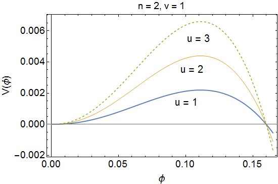
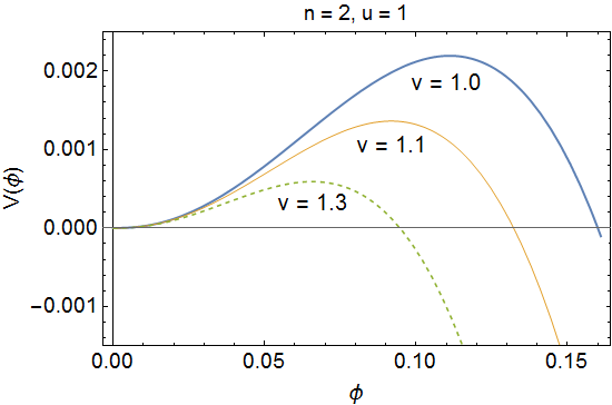
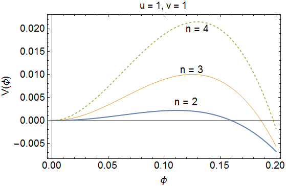
We note that increasing the value of the parameter $u$ corresponds to scaling up the potential, while increasing $v$ corresponds to scaling down the potential as well as making the barrier narrower as seen in Fig. 1. Both of these changes tend to bring down the bounce action. If we fix $u$ and $v$ and vary the parameter $n$, the dependence is more complicated. To take a special case, if we fix $v=1$, we see that as we increase $n$, the barrier width and the barrier height increases (the width asymptotes to a constant) while the bounce action decreases, as shown in Fig. 2. Hence, a higher barrier can result in a lower action, as known from scaling relations [28]. The dependence of bounce action on scaling of barrier parameters will be studied in greater generality in section IV.

We shall now discuss a potential with exact bounce solution which has been known [26].

The bounce solution is given by

Similar to the binomial potential, this potential has a barrier near the false vacuum followed by a run-off for large values of $\phi$. The $\log$ function has a singularity at $\phi=0$, but the potential has a well defined limit at that point. Scaling the parameters $w$ and $m$ correspond to scaling the field-space width of the barrier or scaling the height of the potential (with corresponding changes to the radius-scale $r_{\Sigma}$). How the bounce action depends on these parameters is also clear; the bounce action decreases with the barrier height and increases with the barrier width. We shall generalize this discussion in the next section.

In this section we shall discuss how the scaling of the potential profile along the bounce trajectory (which changes the height and width of the barrier) affects the bounce action. Since this is effectively a single field problem, we shall call the field variable $\phi$, corresponding to either the single field coordinate (for the single field potential) or the arc length along a multi-field trajectory (for the multi-field potential). The potential profile along the trajectory includes the barrier region ($\displaystyle{V>0}$) and also the region beyond it ($\displaystyle{V<0}$).

Let us start with a tunneling potential $V(\phi)$ with a bounce solution $\displaystyle{\bar{\phi}(r)}$ (not necessarily analytic). In order to parametrize scaling, we introduce a variable $\displaystyle{g>0}$, with $\displaystyle{g=1}$ corresponding to the original potential. On changing the value of $g$, let the potential $V$ (barrier height) and the length-scale in field-space $\phi$ (barrier width) scale as powers of $g$, $\displaystyle{g^{a}}$ and $\displaystyle{g^{b}}$ respectively. We denote the rescaled potential and bounce solution as $\displaystyle{V_{g}}$ and $\displaystyle{\bar{\phi}_{g}}$ respectively ($\displaystyle{V_{1}\equiv V}$ and $\displaystyle{\bar{\phi}_{1}\equiv\bar{\phi}}$). We observe that for the scaling to be consistent, the typical radius $r$ must also scale. Collectively, the scaling relations are as follows

In order to ensure that $\bar{\phi}_{g}$ satisfies the equation of motion (1), we must have an additional constraint

This is consistent with the scaling argument presented in [32] for the single-field case. From the scaling relations (24) and (28) and from (2), the bounce action scaling is obtained

We may also check the scaling of the approximation/lower bound (9). Naming this quantity as $\displaystyle{S^{LB}}$, we observe that it scales as $\displaystyle{S_{g}^{LB}=g^{4b-a}S^{LB}}$, which is the same as the bounce action. Therefore, any change in the potential profile and the bounce solution, provided it can be reduced to a scaling of the height of the potential profile and/or a scaling of the field space length scale will maintain the level of accuracy of the approximation. Changes to the shape of the potential profile (which cannot be reduced to some form of scaling) can, however, affect the accuracy of the approximation (9).

Let us now apply the scaling argument for the potentials with exact solutions discussed in section III. For the logarithmic potential (19), if the parameters scale as $w_{g}=g^{\gamma}w$ and $m_{g}=g^{\delta}m$, $\phi$ and $r$ can be rescaled as

to obtain

This gives us all the scaling exponents in (24) and (29). This same approach can be followed for the binomial potential. The results are summarized in Table 1.

We note that the $g$-scaling of the action in Table 1 agrees with the exact expressions (16) and (21) if we plug in the scaling of parameters $u$, $v$, $w$ and $m$. This is necessary to ensure the consistency of the scaling approach.

We shall now discuss the insights gained from the scaling argument regarding the relation between the barrier parameters and the bounce action. We begin by noting that the bounce action scales as $g^{4b-a}$. This means that in general, taller ($a>0$) and narrower ($b<0$) barriers lead to a smaller bounce action. In fact, it is possible to make the barrier larger in all respects (increase in both height and width) and still reduce the bounce action provided the barrier height increases fast enough ($a>4b$) to compensate for the increase in width. The reason for this becomes clear by recalling the estimate (9): the action decreases because the decrease in $r_{\Sigma}^{3}$ is faster than the increase in the surface tension integral.

We note that this is different from the case of non-relativistic quantum mechanics, where barriers with larger surface tension always lead to a larger action due to the absence of the $r^{3}$ factor³³ 3 The surface tension in both cases scales as $\displaystyle{\sigma_{g}=g^{(a+2b)/2}\sigma}$.. Therefore, in the case of multi-field potentials, we cannot assume tunneling happens in the direction of the “smallest” barrier. In section V, using additive potentials, we explicitly show situations where the tunneling trajectory lies in the direction of a larger barrier.

While the scaling argument captures the dependence of action on two barrier parameters (height and width), the actual diversity in the types of potential profiles is far greater than what can be described using only two parameters. Changing the value of $n$ in the binomial potential (14) provides one such example that leads to a non-scaling change in shape of the profile, as seen in Fig. 1. The dependence of barrier parameters and bounce action on $n$ can be seen in Fig. 2. It can be clearly seen that for small values of $n$, the exact bounce action $S$ and the approximation $\displaystyle{S^{LB}}$ scale differently. We note that for $\displaystyle{n\gg 1}$, changing $n$ reduces to a scaling of the potential, which explains why these curves scale the same way for large values of $n$.

One of the simplest ways of going from a single field potential to an $N$-field potential is by defining an additive potential

Owing to the fact that the different field coordinates $\phi_{i}$ behave as independent, uncoupled fields, the $N$ equations (5) completely decouple to give $N$ independent single field equations of motion of the type (1).

For simplicity, let us assume that each of the $\displaystyle{V_{i}}$’s has a non-trivial tunneling solution $\displaystyle{\bar{\phi}_{i}(r)}$ apart from the trivial one ($\displaystyle{\phi_{i}(r)=0}$). This means that the there are $\displaystyle{2^{N}-1}$ solutions for the $N$-field bounce, corresponding to each field picking either the trivial or non-trivial solution⁴⁴ 4 We discount the solution $\phi_{i}(r)=0\;\forall\,i$ which does not involve tunneling out of the false vacuum..

For additive potentials, the action for $N$-fields is obtained by adding the single field action for each of the $N$ fields (2) which are completely independent of each-other

Since each of the $S_{i}$’s can be either positive or $0$, the lowest action is provided by the solution where one of the $S_{i}$’s takes the smallest non-trivial value and all others are $0$; this is the bounce action.

Effectively, tunneling happens along (or is dominated by) a field axis which corresponds to the $V_{i}$ that minimizes the bounce action among the $N$ choices available. This does not have to correspond to the axis with the smallest barrier. For example, let us consider an $N$-field potential where each of the $V_{i}$’s is a binomial potential (14) with the same value of $n$ but with different $u$ and $v$ (which scale as powers of $g$). If the exponents in Table 1 are such that $\displaystyle{\left\{\alpha>0,\hskip 0.28453pt\beta<0\right\}}$ and $\displaystyle{\alpha>(2n-1)|\beta|}$, the axis corresponding to highest value of $g$ would dominate tunneling. This is not the direction with the smallest barrier as all of the other field axes have shorter and narrower barriers.

We may study the dependence of the bounce action on the number of fields $N$ to see how $N$ affects vacuum metastability. The answer will depend on what class of additive potentials we consider, i.e., what restrictions we put on them. Let us consider building an $N$-field additive potential of the form (34), starting from individual single field components $V_{i}(\phi_{i})$. For simplicity, we assume the $V_{i}$’s are all potentials of the same type (for example, potentials such as (14) or (19)) differing only in the choice of parameters (such as $u$, $v$, $m$ or $w$), which could all be selected from random distributions. By this choice, we are requiring that the potential profile along each of the axes will have the same shape (but can have different scaling).

We shall try to enforce some measure of $N$-independence in the potential that we construct by requiring that for any $N$, the typical values of the potential (heights of its peaks and valleys) at typical points on the unit $\displaystyle{N-1}$ sphere in field-space must be $N$-independent. This constraint is inspired by a similar approach in [23] for the case of quartic potentials. Points on the unit sphere can be parametrized as $\displaystyle{\vec{\phi}=\frac{1}{\sqrt{N}}(c_{1},c_{2},...,c_{N})}$, where each of the $\displaystyle{c_{i}}$’s are typically $O(1)$⁵⁵ 5 Points on the unit-sphere also satisfy $\displaystyle{\displaystyle\sum\limits_{i=1}^{N}c_{i}^{2}=N}$..

Since the potential is additive, we require each component potential $\displaystyle{V_{i}(c_{i}/\sqrt{N})}$ to scale as $1/N$, so that the overall potential (at typical points) does not scale with $N$. Therefore, by imposing this particular form of $N$-independence in the potential, we are forced to choose parameters ($u$, $v$, etc.) from distributions such that the $V_{i}$’s and the length-scales of the $\phi_{i}$ axes scale with $N$.

From the arguments in the preceding section, we know that tunneling happens along a field axis (the one which minimizes the action). Therefore, the barrier height and barrier width on the tunneling trajectory also scale as $1/N$ and $1/\sqrt{N}$, respectively (due to the fact that a field axis is not a typical direction). Here $N$ plays the role of $g$ in our scaling arguments, and we are left with the scaling exponents $\displaystyle{a=-1/2}$ and $\displaystyle{b=-1}$. This automatically fixes $c=0$, i.e., the typical bounce radius is $N$-independent. The exact bounce action (2) scales as $N^{-1}$, and so does the approximation (9). Thus, for these potentials, tunneling probability is enhanced as $N$ grows. This agrees with the result found in [23] where the action scales as $N^{-\alpha}$ with $\alpha>1$.

In the case of additive potentials, the bounce solution satisfies the longitudinal equation of (6) because it is effectively a single field bounce. The transverse equation is trivially satisfied because the path is a straight line and the variation of the potential in all the remaining $N-1$ directions is also $0$ (all the remaining field coordinates rest at a minimum of their potential)⁶⁶ 6 Note that for the non-axis solutions to (5), the LHS and RHS of the second equation are typically nonzero..

When we move away from additive potentials to potentials with cross-couplings, the story becomes considerably more complicated. For such potentials, straight line directions with no transverse gradients do not generally exist which makes it difficult to identify solutions that satisfy both equations (6). However, if we are able to identify the bounce trajectory, it is possible to compute either the exact action (2) or its approximation (9), both of which scale the same way.

Greene et al. [23] sought to make the multi-field tunneling problem tractable for quartic potentials by calculating estimate (9) in two steps. In one step, they assumed that the potential profile of the trajectory corresponds approximately to a straight-line path and studied the variation of the bubble radius (presumably $r_{\Sigma}$ or something similar) for quartic potential profiles. They observed that the radius usually took on values within the same order of magnitude for a distribution of sampled potentials and therefore attributed a standardized value of radius for their bounce action estimate. In the second step, they calculated the surface tension integral for the most “obvious” choice of tunneling trajectory, the one passing through the smallest surface tension barrier. Our arguments indicate that this step is not justified as it may pick the wrong tunneling direction/trajectory.

Using a code improvised from [29], we computed the exact action for two-field potentials in order to compare with the estimate of Greene et al. [23]. For the potentials we considered, their estimate was of the same order of magnitude as the exact bounce action. It would be interesting to check the approximation for larger numbers of fields by numerically computing the bounce action to see if the approximation still agrees.

References

- [1] R. Bousso and J. Polchinski, JHEP 0006, 006 (2000) [hep-th/0004134].
- [2] J. L. Feng, J. March-Russell, S. Sethi and F. Wilczek, Nucl. Phys. B 602, 307 (2001) [hep-th/0005276].
- [3] S. Sarangi, G. Shiu and B. Shlaer, Int. J. Mod. Phys. A 24, 741 (2009) [arXiv:0708.4375 [hep-th]].
- [4] E. Silverstein and A. Westphal, Phys. Rev. D 78, 106003 (2008) [arXiv:0803.3085 [hep-th]]
- [5] M. C. Johnson and M. Larfors, Phys. Rev. D 78, 083534 (2008) [arXiv:0805.3705 [hep-th]].
- [6] S.-H. Henry Tye, D. Wohns and Y. Zhang, Int. J. Mod. Phys. A 25, 1019 (2010) [arXiv:0811.3753 [hep-th]].
- [7] S.-H. H. Tye and D. Wohns, [arXiv:0910.1088 [hep-th]].
- [8] P. Ahlqvist, B. R. Greene, D. Kagan, E. A. Lim, S. Sarangi and I. S. Yang, JHEP 1103, 119 (2011) [arXiv:1011.6588 [hep-th]].
- [9] V. Balasubramanian, B. Czech, K. Larjo and T. S. Levi, Phys. Rev. D 84, 025019 (2011) [arXiv:1012.2065 [hep-th]].
- [10] B. Czech, Phys. Lett. B 713, 331 (2012) [arXiv:1112.1638 [hep-th]].
- [11] M. Duncan, W. Gu, Y. H. He and D. Zhou, JHEP 1406, 042 (2014) [arXiv:1402.3162 [hep-th]].
- [12] A. D. Linde, Phys. Rev. D 58, 083514 (1998) [gr-qc/9802038].
- [13] B. Freivogel, M. Kleban, M. Rodriguez Martinez and L. Susskind, JHEP 0603, 039 (2006) [hep-th/0505232].
- [14] A. H. Guth, J. Phys. A 40, 6811 (2007) [hep-th/0702178 [HEP-TH]].
- [15] B. Freivogel, Class. Quant. Grav. 28, 204007 (2011) [arXiv:1105.0244 [hep-th]].
- [16] D. Yamauchi, A. Linde, A. Naruko, M. Sasaki and T. Tanaka, Phys. Rev. D 84, 043513 (2011) [arXiv:1105.2674 [hep-th]].
- [17] D. S. Park, JHEP 1201, 165 (2012) [arXiv:1111.2858 [hep-th]].
- [18] K. Sugimura and E. Komatsu, JCAP 1311, 065 (2013) [arXiv:1309.1579 [astro-ph.CO]].
- [19] R. Bousso, D. Harlow and L. Senatore, arXiv:1309.4060 [hep-th].
- [20] R. Bousso, D. Harlow and L. Senatore, arXiv:1404.2278 [astro-ph.CO].
- [21] S. R. Coleman, Phys. Rev. D 15, 2929 (1977) [Erratum-ibid. D 16, 1248 (1977)].
- [22] U. Sarid, Phys. Rev. D 58, 085017 (1998) [hep-ph/9804308].
- [23] B. Greene, D. Kagan, A. Masoumi, D. Mehta, E. J. Weinberg and X. Xiao, Phys. Rev. D 88, no. 2, 026005 (2013) [arXiv:1303.4428 [hep-th]].
- [24] A. Aravind, D. Lorshbough and S. Paban, Phys. Rev. D 89, 103535 (2014) [arXiv:1401.1230 [hep-th]].
- [25] F. Loran, Mod. Phys. Lett. A 22, 2217 (2007) [hep-th/0612089].
- [26] A. Ferraz de Camargo, R. C. Shellard and G. C. Marques, Phys. Rev. D 29, 1147 (1984).
- [27] S. R. Coleman, V. Glaser and A. Martin, Commun. Math. Phys. 58, 211 (1978).
- [28] E. J. Weinberg, Cambridge University Press (2012)
- [29] C. L. Wainwright, Comput. Phys. Commun. 183, 2006 (2012) [arXiv:1109.4189 [hep-ph]].
- [30] A. Masoumi and E. J. Weinberg, Phys. Rev. D 86, 104029 (2012) [arXiv:1207.3717 [hep-th]].
- [31] T. Konstandin and S. J. Huber, JCAP 0606, 021 (2006) [hep-ph/0603081].
- [32] C. Scrucca, http://itp.epfl.ch/webdav/site/itp/users /181759/public/aqft.pdf