Phonon thermal conductivity by non-local non-equilibrium molecular dynamics

Molecular dynamics (MD) simulation applies to crystals provided the temperature $k_{B}T$ is reasonably high on the scale of the lattice energies $\hbar\omega$. Then classical Newtonian trajectories give good thermal averages. Going beyond harmonic lattice dynamics is difficult with quantum mechanics, but easy with classical MD, not requiring perturbation theory. A “direct” simulation of phonon thermal conductivity $\kappa$ by non-equilibrium molecular dynamics (NEMD) was first done by Payton et al. [1] in 1967, and is now common. Good examples are the comparative study by Schelling et al. [2] and the careful study of GaN by Zhou et al. [3]. A difficulty occurs because small $\omega_{Q}$ vibrational modes have long mean free paths $\Lambda_{Q}$, but only modes with $\Lambda_{Q}<L$ (where $L$ is the length of the simulation cell) have their contribution to $\kappa$ correctly treated by NEMD.

Long mean free paths imply non-locality of $\kappa$. Phonons passing through point $x$ bring information about the temperature $T(x^{\prime})$ over distances $|x-x^{\prime}|$ comparable to their mean free path. Non-locality is widely acknowledged[4, 5, 6, 7, 8, 9], but not always considered a direct topic of study. Recent interest in inhomogeneous situations with boundary effects and spatially varying heat input $H(\vec{r})$ gives new impetus to non-local analysis [10, 11, 12, 13, 14, 15, 16]. Homogeneous systems are much simpler; non-locality is easy to include theoretically. A non-local analysis has value that deserves recognition.

In NEMD simulation, heat $H(x)$ is added and subtracted in equal amounts ($\int dxH(x)=0$) at different places $x$. After steady state is achieved, the temperature $T(x)$ is found by averaging over finite discrete sections. Usually the aim is to extract a value of $dT/dx$ from a place distant from sources and sinks of heat. This yields a value $\kappa_{\rm eff}(L)$ for the thermal conductivity, $L$ being the system size. The result is then studied as a function of $L$, to extract the bulk limit $\kappa=\kappa_{\rm eff}(L\rightarrow\infty)$. If heating $|H(x)|$ is weak, response is linear, and the relation $\Delta T(x)=\int dx^{\prime}S(x-x^{\prime})H(x^{\prime})$ must hold. In Fourier variables, this is $\tilde{\Delta}T(q)=\tilde{S}(q)\tilde{H}(q)$. From energy conservation $dJ(x)/dx=H(x)$ and the non-local Fourier law[17] $J(x)=-\int dx^{\prime}\kappa(x-x^{\prime})dT(x^{\prime})/dx^{\prime}$, one finds $\tilde{\kappa}(q)=1/q^{2}\tilde{S}(q)$. The “tilde” is used to indicate when a function is in reciprocal space instead of direct space.

In this paper, we show that we can improve on $\kappa_{\rm eff}(L)$ by thinking non-locally. The results of NEMD calculations can be considered to arise from $\tilde{\kappa}(q)$ for values $q=2\pi n/L$ (for periodically repeated slabs), or $q=\pi n/L$ (for terminated slabs). Here $L$ is the length of the simulation cell. The desired true bulk $\kappa=\tilde{\kappa}(q\rightarrow 0)=\int d\vec{r}\kappa(\vec{r})/V$, requires extrapolation. This extrapolation is best guided by theory aimed at $\tilde{\kappa}(q)$. A useful strategy is therefore direct computation of $\tilde{\kappa}(2\pi/L)$, using this to optimize the extrapolation to $L\rightarrow\infty$. The reason why $\kappa=\tilde{\kappa}(0)$ is unavailable is because $\tilde{H}(0)=\int d\vec{r}H(\vec{r})/V$ must vanish in order for a steady state to be allowed.

This paper does four things. (1) We Fourier-analyze the common version of NEMD where the system is periodic with length $L$ along the direction of heat flow, and heat input and removal occurs in isolated slabs separated by $L/2$. A rigorous relation between $\kappa_{\rm eff}(L)$ and $\tilde{\kappa}(q)$ is worked out. (2) A method is given for direct MD simulation of $\tilde{\kappa}(q)$, by applying and extracting heat in a sinusoidal pattern [4]. This has numerical advantages over other protocols. (3) Convergence of $\tilde{\kappa}(q)$ towards $\kappa$ is studied by NEMD simulation for the Lennard-Jones (LJ) liquid and crystal. (4) The Peierls “Boltzmann Transport Equation” (BTE) [19, 20] is solved for $\tilde{\kappa}(q)$ in Debye approximation ($\omega_{Q}=v|\vec{Q}|$) with $1/\tau_{Q}=(1/\tau_{D})(\omega_{Q}/\omega_{D})^{p}$. The appropriate power $p$ is probably 2. This helps understand convergence as the MD simulation-cell size $L$ increases. For the particular case $p=2$ most often encountered, it is shown that $\kappa_{\rm eff}(L)\sim\kappa-C^{\prime}/\sqrt{L}$, rather than the form $\sim\kappa-C/L$ which has been widely assumed.

Assume a homogeneous single crystal, represented by a simulation cell with periodic boundary conditions. The $i^{\rm th}$ atom at $\vec{r}_{i}$ and the atom at $\vec{r}_{i}+\vec{R}$ are equivalent, and have the same trajectory $\vec{r}_{i}(t)$. For simplicity, the primitive translation vectors $\vec{R}$ of the simulation cell ($\vec{A}_{1},\ \vec{A}_{2},\ \vec{A}_{3}$), are assumed orthogonal. For example, in the sample calculations presented later, they are taken to be $N_{x}a\hat{x},\ N_{y}a\hat{y},\ N_{z}a\hat{z}$, where $a$ is the lattice constant, the edge-length of the fcc conventional cube. A typical cell has size $(N_{x},\ N_{y},\ N_{z})=(80,\ 6,\ 6)$, With 4 atoms in the conventional cube, this means 11,520 atoms. Heating is done in slabs perpendicular to the long vector ${\vec{A}}_{1}$. Therefore, current flows parallel to $\vec{A}_{1}$. This is why a one-dimensional notation ($J(x)$ and $\tilde{\kappa}(q)$, for example) is used. The simulation cell length $L=L_{x}=|\vec{A}_{1}|=N_{x}a$ is chosen as large as computation permits, trying to surpass the distance $\Lambda$ of non-local thermal memory.

Boundaries create challenging problems. Nanoscale heat transfer is typically dominated by thermal boundary (or Kapitza) resistance [21, 22]. For study of bulk conductivity, the aim is to reduce the influence of boundaries. One can argue [23] that periodic boundary conditions are not the most favorable way to do this. However, in this paper, periodicity offers simplicity for analysis, overruling other considerations.

A further simplification follows computational necessity. Discretize the temperature $T(\vec{r})$ into slab values $T(\ell)$. The slabs are layered in the $\vec{A}_{1}$-direction, and have width $d=n_{S}a$ where $n_{S}$ is a small integer and a factor of $N_{x}$. The number of slabs is $N_{S}=N_{x}/n_{S}$. Let the variable $x$ denote distance along the $\vec{A}_{1}$-axis, perpendicular to slabs. The slab indexed by the integer $\ell$ occupies the interval $\ell d-d/2<x<\ell d+d/2$. The temperature $T(\ell)$ is found from the average kinetic energy of the atoms in the $\ell$’th slab. Heat is transferred externally into the $\ell$’th cell at a volume-average rate $H(\ell)$. In steady state, an outward heat flux conserves energy, $H(\ell)=[J(\ell+1/2)-J(\ell-1/2)]/d$. Both current and temperature gradient are properties of the junction of two adjacent slabs. Their steady-state linear relation is $J(\ell+1/2)=-\sum_{\ell^{\prime}}\kappa(\ell,\ell^{\prime})\nabla T(\ell^{\prime}+1/2)$, where the sum runs over the $N_{S}$ slabs. This definition is required by linear math. Periodicity requires $\kappa(\ell,\ell^{\prime})=\kappa(\ell+mN_{S},\ell^{\prime}+nN_{S})$, and homogeneity (if the medium is in fact homogeneous) requires that $\kappa(\ell,\ell^{\prime})=\kappa(\ell-\ell^{\prime})$. Corresponding (via a unitary Fourier transformation) to the $N_{S}$ distinct slabs, there are $N_{S}$ distinct wave-vectors $q_{n}=2\pi n_{q}/N_{S}d=2\pi n_{q}/L$, indexed by integers $n_{q}$ ($|n_{S}|\leq N_{S}/2$), and distributed in a one-dimensional Brillouin zone. In the homogeneous case, the relation is $\tilde{J}(q)=-\tilde{\kappa}(q)\tilde{\nabla}T(q)$. These ideas were introduced in Ref. 4, where further properties are explained.

It is not hard to extend the usual derivation of the Kubo formula (ref. 24, for example) to derive a Kubo formula for $\kappa(x,x^{\prime})$ or $\kappa(\ell,\ell^{\prime})$. The classical limit is

A common version of NEMD simulation removes energy only from slab $\ell=0$, at a volume-average rate $H$, and inserts energy at the same rate into slab $\ell=N_{S}/2$. Zhou et al. [3] did a careful study of $\kappa$ for GaN by this method. They discuss, but do not completely resolve, the issue of how the answer for $\kappa$ scales with system size. Here we analyze this version with periodic boundaries ($\ell=\ell+N_{S}$), rather than the rigid or free boundaries sometimes used. Heat current $J_{x}(\ell+1/2)=\pm(d/2)H\equiv\pm J$ flows across slab boundaries, the plus sign for $\ell$ to the right of the input and left of the output slab, and the minus sign for opposite cases. Thermal conduction is found using the relation $\kappa_{\rm eff}(L)\equiv-J/\nabla_{x}T({\rm mid})$. The rigorous non-local Fourier law is $\tilde{J}(q_{n})=-\tilde{\kappa}(q_{n})\tilde{\nabla}T(q_{n})$. Analysis given in Appendix B shows that

where the subscript on $q_{n}$ has been dropped. This holds if $N_{S}/4$ is an integer. If it is a half-integer, then $\cos(qd/2)$ is replaced by 1. Liquids have a very local conductivity, where $\tilde{\kappa}(q)\approx\kappa$ is nearly independent of $q$. Then the sum in Eq.(2) converges correctly to $\kappa_{\rm eff}\rightarrow\kappa$ without needing a small $q_{1}=q_{\rm min}=2\pi/L$. For crystals like GaN, where non-local behavior is caused by long mean free paths of small-$Q$ phonons, $\tilde{\kappa}(q)$ peaks around $|q|=0$. Accurate results require a small $q_{\rm min}$ or a large $L$. When $q_{\rm min}$ is not very small, the first two terms $n_{q}=\pm 1$ in Eq.(2) dominate. Approximating $\sin(q_{\rm min}d/2)$ by $\pi/N_{S}$ and $\cos(q_{\rm min}d/2)$ by 1, the result is $\kappa_{\rm eff}\approx\pi\tilde{\kappa}(q_{\rm min})/4$, which is smaller than $\pi\kappa/4$ (and still smaller than the true $\kappa$.) It would be better to calculate $\tilde{\kappa}(q_{\rm min})$ directly. A method is given in the next section.

The simulation cell is divided into slabs centered at $x(\ell)=\ell d,\ \ell=1,\ldots,N_{S}$. It is shown schematically in Fig. 1. The distance $d=L/N_{S}$ is the width of a slab. It is a multiple of $a=L/N_{x}$ where $N_{x}a=L$ is the repeat distance on the long axis. We want to modify the heat input profile. Instead of the two slab version, let the heat input be of the form $H(\ell)=\tilde{H}(q_{\rm min})\cos(q_{\rm min}x(\ell))$. The temperature variation then has the form $T(\ell)=T_{0}+\tilde{\Delta}T(q_{\rm min})\cos(q_{\rm min}x(\ell))$. Since slab temperatures $T(\ell)$ at all of the $N_{S}$ different values of $\ell$ are used to compute the Fourier amplitude $\tilde{\Delta}T(q_{\rm min})$, numerical noise averages out faster.

Equation 26 of the previous paper [4] says, for arbitrary heating $H(\ell)$, heating rate, temperature, and conductivity in Fourier space are related by (for $q\neq 0$),

For simple sinusoidal heating, $\tilde{H}(q)$ and $\tilde{\Delta}T(q)$ are zero except at $q=q_{\rm min}$, where their values are denoted as $H$ and $\Delta T$. Then the thermal conductivity is

This makes sense: $2\pi\Delta T/N_{S}d$ is the maximum temperature gradient, and $HN_{S}d/2\pi$ is the maximum heat current.

Now we need a good numerical algorithm to drive the oscillatory heat input. Furtado, Abreu, and Tavares[2] (FAT) made an improvement on the popular algorithm by Müller-Plathe [26]. The usual Müller-Plathe method gives equal heating and cooling to two chosen slabs. The hottest atom in the slab chosen for heat removal, and the coldest atom in the slab for heat insertion, have their velocities interchanged, conserving energy and momentum. The FAT algorithm does not interchange velocities. It is decided in advance what heat $\Delta\epsilon$ should be added and subtracted. Then a corresponding velocity increment $\Delta\vec{v}$ is added to one of the two atoms, and subtracted from the other, in such a way that total energy and momentum are conserved, local energy being altered by $\pm\Delta\epsilon$. The minimum possible magnitude $|\Delta\vec{v}|$, is chosen, so that the resulting disruption is minimized. This allows heat input at a predetermined rate which can be spatially varied. Details are given in the on-line supplemental material[27].

The Lennard-Jones (LJ) liquid is a simple case, used by Müller-Plathe [26] to test his algorithm. The pair potential is

The parameters for argon [28] are $\epsilon/k_{B}=119.6$K and $\sigma$ =3.405Å. First, we use Müller-Plathe’s algorithm to reproduce his results, at the same $(N,V,T)$= 2592 atoms, $\rho=N/V=0.849/\sigma^{3}$, and $T=0.7\epsilon/k_{B}=$84K. The same simulation cell is used, consisting of $18\times 6\times 6$ fcc conventional cubes, and periodic boundary conditions. The cut-off distance for the LJ potential is $3.0\sigma$. We get the same answer, $\kappa$=7.1 in LJ units.

As shown in Fig. 2 of ref. 26, and confirmed by our calculation in Fig. 2, the temperature gradient is essentially constant all the way to, and including, the slabs $0$ and $N_{S}/2=10$. This is because thermal conductivity in a liquid is very local. This can be contrasted with Fig. 2 of ref. 3 or Fig. 4 of ref. 4, for crystals with non-local $\kappa$. Gas theory is certainly not correct for a liquid; the concept of a mean-free path is not valid. However, we can get an idea of what happens by unlicensed use of the gas formula $\kappa=C{\bar{v}}\Lambda/3$. The measured thermal conductivity of liquid argon (0.132 W/mK at temperature near 100K and pressure near 1Mbar [29, 30, 31, 32]) then corresponds to a mean free path $\Lambda\approx 0.14\ \AA$, more than 30 times smaller than the slab separation $a=1.68\sigma$. In other words, the non-local conductivity $\kappa(z-z^{\prime})$ decays to zero by the first neighbor slab, or $\tilde{\kappa}(q)$ is independent of $q$ out to values of $q$ larger than $q_{\rm max}=\pi/d$.

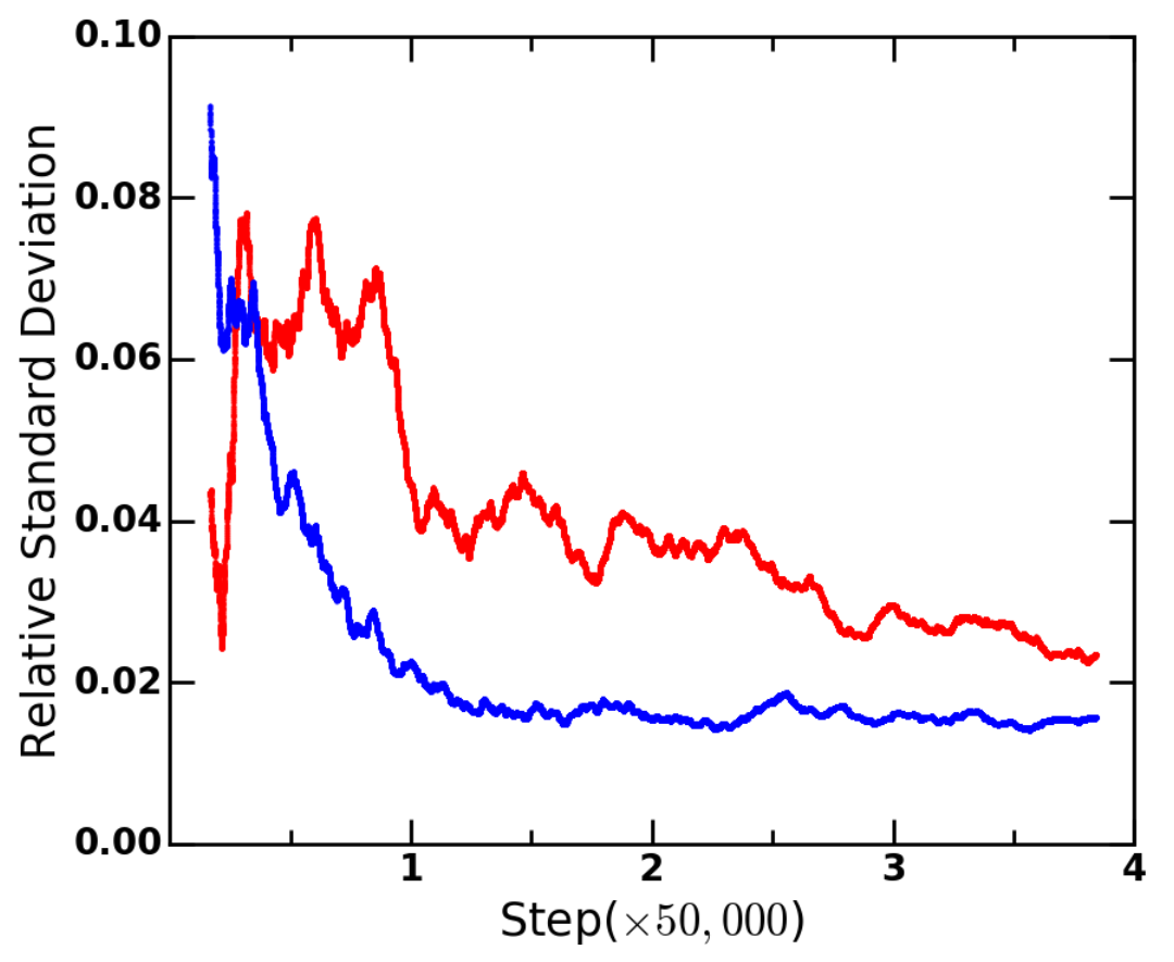
Also shown in Fig. 2 is the sinusoidal temperature profile gotten numerically from our sinusoidal heating. The computational system is unaltered. The 2592 atoms are in the same cell, divided into 20 slabs, at the same $T$. Heat $H(\ell)=H\cos(2\pi\ell/N_{S})$ was inserted, with $H$ between 1 and 5 $\epsilon/(\Delta t\cdot{\rm slab})$. Slabs were heated by choosing “adjoint” slabs ($\ell$ and $\ell+N_{S}/2$), finding coolest and hottest atoms, and altering the kinetic energies sinusoidally by use of the FAT algorithm. This was done for all slabs simultaneously, at a fixed time step ($\Delta t=15\delta t$ for short samples and $60\delta t$ for long samples). The time step $\delta t$ used for the “velocity Verlet” Newton’s-law integration algorithm [33, 34] is $\delta t=0.007t_{LJ}$. The LJ unit of time for argon is $t_{LJ}=\sigma\sqrt{(}m/\epsilon)=2.16$ ps. Equilibration required $10^{4}\ \delta t$ of constant $T$ simulation, and $T(\ell)$ averaging was done for $2\times 10^{5}\delta t$; good convergence was found in $5\times 10^{4}\delta t$ as shown in Fig. 3.

To estimate errors, consider that there are 130 atoms per slab, each with mean energy $k_{B}T$ and rms deviation of $k_{B}T$ from the mean, according to Maxwell-Boltzmann statistics. Thus the mean slab energy per atom, at any particular moment, should be about $k_{B}T\pm k_{B}T/\sqrt{1}30$ Therefore, if averaged over 100 random and independent thermalized configurations, the temperature error in a slab will be less than 1%. A run of $5\times 10^{4}\delta t$ should be more than sufficient for this purpose. Fig. 2 suggests errors of order 0.001$k_{B}T$ in the slab temperatures.

Both of the current LJ liquid simulations give the same value, $\kappa$ = 7.1 in LJ units, equal to the Müller-Plathe [26] result. In normal units, this is 0.133 W/mK, very close to the experimental value for argon, 0.132 W/mK [29, 30, 31, 32]. The sinusoidal algorithm gives faster convergence and a slightly more accurate final answer, as shown in Fig 3.

NEMD answers for $\kappa$ are computed for finite size $L$. Therefore extrapolation is required to estimate the bulk ($L\rightarrow\infty$) answer. Sellan et al. [5] have analyzed this. It was also analyzed in the previous paper [4], using a Debye model. Here we continue the analysis. Equations (22,23) of ref. 4 are

where $v_{Qx},\ \tau_{Q}$, and $\Lambda_{Qx}=v_{Qx}\tau_{Q}$ are the group velocity, quasiparticle lifetime, and $x$-component of mean free path of the phonon mode of frequency $\omega_{Q}$. The sum over modes $Q$ implicitly includes a sum over branches. These equations solve the BTE in relaxation-time approximation (RTA; also known as the “Single Mode Approximation”) for the case where heat is applied as $H(\ell)\propto\cos(q\ell d)$. We focus on the smallest $q$, $2\pi/L$.

Recent progress in numerical solution of the BTE [36, 37, 38, 39] has enabled comparison of RTA against exact solutions. Very often, RTA answers are accurate at room temperature, graphene [40, 41] being a notable exception. Here we adopt both the RTA and the overly simplistic Debye model. The aim is not an accurate $\kappa$, only insight about the size-dependence of $\kappa(q_{\rm min}=2\pi/L)$, to guide extrapolation to the $L\rightarrow\infty$ limit. We choose the mean free path $\Lambda_{Qx}$ to scale as $Q^{-p}$,

Then Eqns.(6, 7) become

Here the sum over $Q$ contains an explicit factor of 3, for the three acoustic branches, all given the same velocity $v$ in the Debye model; $\kappa_{0}$ is a convenient scale factor,

This is just the classical limit of the standard formula $(1/3)Cv\ell$ with $\ell=v\tau_{D}$. The Debye wavevector has its usual value, $(6\pi^{2}N/\Omega)^{1/3}$. A common choice for the exponent is $p=2$.

Here, instead of integrating over the Debye sphere, we use direct numerics to do the discrete sum of Eq. 9 over the actual discrete $Q$-mesh in the Brillouin zone of the fcc simulation cell that will be used in the next section for the LJ crystal. That is, we use only those $\vec{Q}$’s in the fcc Brillouin zone such that $\exp(i\vec{Q}\cdot\vec{A}_{i})=1$, where $\vec{A}_{i}$, for $i=1,2,3$, are the orthogonal translation vectors of the simulation supercell. As an example, the mesh used in Sec. V for the LJ liquid corresponds to $\vec{A}_{1}=18a(1,0,0)$, $\vec{A}_{2}=6a(0,1,0)$, and $\vec{A}_{3}=6a(0,0,1)$, where $a=1.68\sigma$ is the lattice constant of the fcc conventional cubic cell, using the liquid argon density, 0.849/$\sigma^{3}$. Our simulation cells in this and the next section will be very similar, but longer in the $\vec{A}_{1}$ direction, and with $a$ readjusted to $1.56\sigma$ to give the higher density[34, 42], 1.053/$\sigma^{3}$, of the low pressure LJ crystal. The corresponding $\vec{Q}$’s are the vectors $\ell\vec{G}_{1}+m\vec{G}_{2}+n\vec{G}_{3}$ of the lattice reciprocal to the $\vec{A}$’s. This is an anisotropic reciprocal-space mesh, being coarse in the directions $\vec{A}_{2}$ and $\vec{A}_{3}$, but finer in the direction $\vec{A}_{1}$, corresponding to the actual distribution of normal modes of the atoms in the simulation cell of the LJ crystal (where $|\vec{G}_{2,3}|$ is larger than $|\vec{G}_{1}|$.) We are guessing that the Debye model, with frequency $\omega_{Q}=v|\vec{Q}|$ for all 3 branches, and $1/\tau_{Q}=(1/\tau_{D})(Q/Q_{D})^{2}$, sufficiently captures the physics of the LJ crystal for purposes of learning how to extrapolate to infinite simulation cell size.

Results are shown in Fig. 4 and in Appendices C and D. The figure shows two things. First, quite smooth extrapolation to the correct $q=0$ answer appears when $\kappa(q)$ is plotted versus $\sqrt{qa}$, as anticipated in Refs. 5 and 4, and clarified in Appendix A. Second, an unexpected divergence (of the form $1/\sqrt{qa}$ begins to appear for cells with small enough $q$ (relative to the transverse size $q_{\perp}\approx 2\pi/N_{y\ {\rm or}\ z}$.) Specifically, the onset of the upward turn appears roughly when $\sqrt{(}qa)<1/2N_{y}$, which corresponds to $N_{x}>25N_{y}^{2}$, a limit not always achieved in NEMD calculations. The origin and significance of this divergence is discussed in Appendix C. The idea for extrapolation is discussed in the caption to Fig. 4 and in Appendix D.

Unlike the LJ liquid, for an LJ crystal, phonon gas theory applies well, but only up to half the melting temperature, where higher-order anharmonic terms become important [16]. This non-Boltzmann regime is where an MD simulation is worth doing . The resulting shorter phonon mean free paths permit shorter simulation cells. We simulate crystalline LJ argon at $T$=80K, close to the experimental triple point (84K and 0.7 atmospheres) and atmospheric pressure melting temperature (84K).

Higher energy phonons have mean free paths a bit longer than the unit cell $a=5.32\AA$, which we choose to be the slab thickness $d$. Lower energy phonons have mean free paths $\Lambda_{Q}$ increasing, roughly as $1/\omega_{Q}^{2}$. The values of $\Lambda_{Q}$ are not as long as in GaN, modeled by Zhou et al. [3]. Nevertheless, doing a converged calculation by MD methods is challenging. We use this to test whether our algorithm is helpful. We use a time step of the “velocity Verlet” Newton’s-law integration algorithm [33, 34] $\delta t=0.007t_{LJ}$ for smaller-size samples, and $0.014t_{LJ}$ for larger ones.

Figs.5 and 6 show results for $\kappa(q=2\pi/L)$ where $L=N_{x}d$ is the length of the simulation cell, and $d=a$. These calculations use a heat input $H(\ell)\Delta t$ (per slab) of $1.265\epsilon\cos(2\pi\ell/N_{S})$. The interval $\Delta t$ between heat insertions is $60\delta t$. The value of $\kappa$ in argon at $T=$80 K is measured [43] to be in the range 0.4 to 0.6 W/mK. Christen and Pollack [44] found $\kappa(80K)\approx 0.30$ W/mK. Fig. 5 looks as if it might extrapolate linearly in the region $qa<0.1$ to a value around 23 in LJ units, whereas Fig. 6 seems more convincingly linear in $\sqrt{(}qa)$, extrapolating to a value $\kappa(q=0)\approx$ 26 in LJ units. The LJ unit of thermal conductivity is $(k_{B}/\sigma^{2})\sqrt{(}\epsilon/M)$=0.0188 /W/mK. Our LJ crystal simulation thus gives $\kappa\approx$ 0.49 W/mK. This compares with the value $0.16-0.17$ W/mK found by Turney et al. [16], 0.236 W/mK found by Omini and Sparavigna [36], 0.25 W/mK found (at 69.2K) by Kaburaki et al. [45], $0.33-0.49$ W/mK (depending on density) found by Christen and Pollack [44], and 0.19 W/mK found by Chernatynskiy and Phillpot [46].

The algorithm of Sec. IV works smoothly and converges more rapidly than the common two-slab heating. It generates a reliable value of $\tilde{\kappa}(q=2\pi/L)$. The macroscopic conductivity, $\kappa={\rm Lim}_{q\rightarrow 0}\tilde{\kappa}(q)$, found by extrapolating the long sample dimension to $L\rightarrow\infty$, is problematic, although less so than for the discrete-slab heating algorithm. Even if Boltzmann transport theory fails because phonon mean free paths are so short that quasiparticles are not well-defined, nevertheless, Boltzmann theory should correctly model the long-wavelength phonon contribution to $\kappa(q)$, which is the problematic part.

Our analysis using the BTE reveals two effects responsible for slower than expected convergence of $\tilde{\kappa}(q)$ to $\kappa$. These are an inevitable correction which scales as $\sqrt{(}qa)$, and the anisotropic mesh artifact that scales as $1/[N_{y}N_{z}\sqrt{(}qa)]\propto\sqrt{(}N_{x})/N_{y}N_{z}$. These are found by numerical summation of the Boltzmann-Debye RTA version, but should faithfully model the effects seen in NEMD models. Simple graphical extrapolation to $q=0$ by assuming linear behavior in $\sqrt{qa}$ is less justifiable than had been hoped, because the contamination by the $1/\sqrt{(}qa)$ term alters the appearance of the $\kappa(q)$ versus $\sqrt{(}qa)$ graph. The cure is to be sure that the ratio $\sqrt{(}N_{x})/N_{y}N_{z}$ does not get too small. Appendix D discusses this further. There are reasons for mild insecurity on the issue of to what extent extrapolation is justified.

References

- [1] D. N. Payton, M. Rich, and W. M. Visscher, Phys. Rev. 160, 706 (1967), URL http://link.aps.org/doi/10.1103/PhysRev.160.706.
- [2] P. K. Schelling, S. R. Phillpot, and P. Keblinski, Phys. Rev. B 65, 144306 (2002), URL http://link.aps.org/doi/10.1103/PhysRevB.65.144306.
- [3] X. W. Zhou, S. Aubry, R. E. Jones, A. Greenstein, and P. K. Schelling, Phys. Rev. B 79, 115201 (2009), URL http://link.aps.org/doi/10.1103/PhysRevB.79.115201.
- [4] J. Sussmann and A. Thellung, Proceedings of the Physical Society 81, 1122 (1963).
- [5] I. B. Levinson, Soviet Physics JETP 52, 704 (1980), URL http://www.jetp.ac.ru/cgi-bin/e/index/e/52/4/p704?a=list.
- [6] T. E. Wilson, F. M. Lurie, and W. E. Bron, Phys. Rev. B 30, 6103 (1984), URL http://link.aps.org/doi/10.1103/PhysRevB.30.6103.
- [7] U. Happek, T. Holstein, and K. F. Renk, Phys. Rev. B 34, 8898 (1986), URL http://link.aps.org/doi/10.1103/PhysRevB.34.8898.
- [8] G. D. Mahan and F. Claro, Phys. Rev. B 38, 1963 (1988), URL http://link.aps.org/doi/10.1103/PhysRevB.38.1963.
- [9] G. G. Chen, J. Heat Transfer 118, 539 (1996), URL http://dx.doi.org/10.1115/1.2822665.
- [10] M. E. Siemens, Q. Li, R. Yang, K. A. Nelson, E. H. Anderson, M. M. Murnane, and H. C. Kapteyn, Nature Materials 9, 26 (2010).
- [11] J. A. Johnson, A. A. Maznev, J. Cuffe, J. K. Eliason, A. J. Minnich, T. Kehoe, C. M. S. Torres, G. Chen, and K. A. Nelson, Phys. Rev. Lett. 110, 025901 (2013), URL http://link.aps.org/doi/10.1103/PhysRevLett.110.025901.
- [12] K. T. Regner, A. J. H. McGaughey, and J. A. Malen, Phys. Rev. B 90, 064302 (2014), URL http://link.aps.org/doi/10.1103/PhysRevB.90.064302.
- [13] A. A. Maznev, J. A. Johnson, and K. A. Nelson, Phys. Rev. B 84, 195206 (2011), URL http://link.aps.org/doi/10.1103/PhysRevB.84.195206.
- [14] Y. K. Koh, D. G. Cahill, and B. Sun, Phys. Rev. B 90, 205412 (2014), URL http://link.aps.org/doi/10.1103/PhysRevB.90.205412.
- [15] J. Maassen and M. Lundstrom, Journal of Applied Physics 117, 135102 (2015), URL http://scitation.aip.org/content/aip/journal/jap/117/13/10.1063/1.4916245.
- [16] J. E. Turney, E. S. Landry, A. J. H. McGaughey, and C. H. Amon, Phys. Rev. B 79, 064301 (2009), URL http://link.aps.org/doi/10.1103/PhysRevB.79.064301.
- [17] Recent literature often claims that thermal conduction in inhomogeneous systems disobeys the Fourier law. It would be better to say that it disobeys the local Fourier law , or . The same J. Fourier who realized also invented the Fourier transforms used here.
- [18] P. B. Allen, Phys. Rev. B 90, 054301 (2014), URL http://link.aps.org/doi/10.1103/PhysRevB.90.054301.
- [19] R. E. Peierls, Ann. Phys. 395, 1055 (1929), URL http://dx.doi.org/10.1002/andp.19293950803.
- [20] J. Ziman, Electrons and Phonons (Oxford, London, 1960).
- [21] E. T. Swartz and R. O. Pohl, Rev. Mod. Phys. 61, 605 (1989), URL http://link.aps.org/doi/10.1103/RevModPhys.61.605.
- [22] D. G. Cahill, P. V. Braun, G. Chen, D. R. Clarke, S. Fan, K. E. Goodson, P. Keblinski, W. P. King, G. D. Mahan, A. Majumdar, et al., Applied Physics Reviews 1, 011305 (2014), URL http://scitation.aip.org/content/aip/journal/apr2/1/1/10.1063/1.4832615.
- [23] Z. Liang and P. Keblinski, Phys. Rev. B 90, 075411 (2014), URL http://link.aps.org/doi/10.1103/PhysRevB.90.075411.
- [24] P. B. Allen and J. L. Feldman, Phys. Rev. B 48, 12581 (1993), URL http://link.aps.org/doi/10.1103/PhysRevB.48.12581.
- [25] F. A. Furtado, C. R. A. Abreu, and F. W. Tavares, AIChE Journal 61, 2881 (2015), ISSN 1547-5905, URL http://dx.doi.org/10.1002/aic.14803.
- [26] F. Müller-Plathe, The Journal of chemical physics 106, 6082 (1997).
- [27] The Furtado et al. paper (Ref.2) appeared after our own version of the algorithm was posted at arXiv:1412.3099. We concede priority, and offer our original description of the method for choosing in the online supplemental material.
- [28] A. Michels, H. Wijker, and H. Wijker, Physica 15, 627 (1949), ISSN 0031-8914, URL http://www.sciencedirect.com/science/article/pii/0031891449901196.
- [29] B. Younglove and H. J. Hanley, Journal of physical and chemical reference data 15, 1323 (1986).
- [30] G. A. Cook, Argon, Helium, and the Rare Gases (Intersciences, New York, 1961).
- [31] H. J. Hanley, R. D. McCarty, and W. M. Haynes, Journal of Physical and Chemical Reference Data 3, 979 (1974).
- [32] H. Ziebland and J. T. A. Burton, British Journal of Applied Physics 9, 52 (1958), URL http://stacks.iop.org/0508-3443/9/i=2/a=302.
- [33] J.-P. Hansen and L. Verlet, Phys. Rev. 184, 151 (1969), URL http://link.aps.org/doi/10.1103/PhysRev.184.151.
- [34] M. E. Tuckerman, B. J. Berne, and G. J. Martyna, The Journal of chemical physics 94, 6811 (1991).
- [35] D. P. Sellan, E. S. Landry, J. E. Turney, A. J. H. McGaughey, and C. H. Amon, Phys. Rev. B 81, 214305 (2010), URL http://link.aps.org/doi/10.1103/PhysRevB.81.214305.
- [36] M. Omini and A. Sparavigna, Physica B: Condensed Matter 212, 101 (1995), ISSN 0921-4526, URL http://www.sciencedirect.com/science/article/pii/0921452695000163.
- [37] D. A. Broido, M. Malorny, G. Birner, N. Mingo, and D. A. Stewart, Applied Physics Letters 91, 231922 (2007), URL http://scitation.aip.org/content/aip/journal/apl/91/23/10.1063/1.2822891.
- [38] W. Li, J. Carrete, N. A. Katcho, and N. Mingo, Computer Physics Communications 185, 1747 (2014), ISSN 0010-4655, URL http://www.sciencedirect.com/science/article/pii/S0010465514000484.
- [39] G. Fugallo, M. Lazzeri, L. Paulatto, and F. Mauri, Phys. Rev. B 88, 045430 (2013), URL http://link.aps.org/doi/10.1103/PhysRevB.88.045430.
- [40] L. Lindsay, D. A. Broido, and N. Mingo, Phys. Rev. B 82, 115427 (2010), URL http://link.aps.org/doi/10.1103/PhysRevB.82.115427.
- [41] G. Fugallo, A. Cepellotti, L. Paulatto, M. Lazzeri, N. Marzari, and F. Mauri, Nano Letters 14, 6109 (2014), pMID: 25343716, URL http://dx.doi.org/10.1021/nl502059f.
- [42] A. Ladd and L. Woodcock, Molecular Physics 36, 611 (1978), URL http://dx.doi.org/10.1080/00268977800101791.
- [43] F. Clayton and D. N. Batchelder, Journal of Physics C: Solid State Physics 6, 1213 (1973), URL http://stacks.iop.org/0022-3719/6/i=7/a=012.
- [44] D. K. Christen and G. L. Pollack, Phys. Rev. B 12, 3380 (1975), URL http://link.aps.org/doi/10.1103/PhysRevB.12.3380.
- [45] H. Kaburaki, J. Li, S. Yip, and H. Kimizuka, Journal of Applied Physics 102, 043514 (2007), URL http://scitation.aip.org/content/aip/journal/jap/102/4/10.1063/1.2772547.
- [46] A. Chernatynskiy and S. R. Phillpot, Phys. Rev. B 82, 134301 (2010), URL http://link.aps.org/doi/10.1103/PhysRevB.82.134301.
On-line Supplemental Material for
- [1] B.-Y. Cao and Y.-W. Li, The Journal of Chemical Physics 133, 024106 (2010), URL http://scitation.aip.org/content/aip/journal/jcp/133/2/10.1063/1.3463699.
- [2] F. A. Furtado, C. R. A. Abreu, and F. W. Tavares, AIChE Journal 61, 2881 (2015), ISSN 1547-5905, URL http://dx.doi.org/10.1002/aic.14803.
- [3] Y. Li and P. B. Allen, arXiv:1412.3099v1 (2014).
- [4] P. B. Allen, Phys. Rev. B 90, 054301 (2014), URL http://link.aps.org/doi/10.1103/PhysRevB.90.054301.
- [5] D. P. Sellan, E. S. Landry, J. E. Turney, A. J. H. McGaughey, and C. H. Amon, Phys. Rev. B 81, 214305 (2010), URL http://link.aps.org/doi/10.1103/PhysRevB.81.214305.