Ab-initio molecular dynamics simulation of liquid water by Quantum Monte Carlo
Abstract
Although liquid water is ubiquitous in chemical reactions at roots of life and climate on the earth, the prediction of its properties by high-level ab initio molecular dynamics simulations still represents a formidable task for quantum chemistry. In this article we present a room temperature simulation of liquid water based on the potential energy surface obtained by a many-body wave function through quantum Monte Carlo (QMC) methods. The simulated properties are in good agreement with recent neutron scattering and X-ray experiments, particularly concerning the position of the oxygen-oxygen peak in the radial distribution function, at variance of previous Density Functional Theory attempts. Given the excellent performances of QMC on large scale supercomputers, this work opens new perspectives for predictive and reliable ab-initio simulations of complex chemical systems.
The simulation by first principles of liquid water, the key element of human life and biological processes, has been a dream for several decades after the foundation of Density Functional theory (DFT), even within the restriction of the Born-Oppenheimer approximation for the heavy nuclei. Realistic simulations are particular important because, at the experimental level, it is not possible to clarify completely what are the relationships between the so many different and rich phases of water and the physical interactions between water molecules, determined by hydrogen bonding and weak long-range van der Waals (vdW) interactions. Moreover water is involved in many biological and chemical processes, and first principle simulations are useful to investigate and rationalize such important mechanisms.
The first attempted simulations date back to the pioneer works by Car and Parrinello[1, 2, 3], within an efficient ab-initio molecular dynamics (AIMD) based on DFT. The comparison with the experiments, at that time available, provided a pretty good agreement with the oxygen-oxygen (O-O) radial distribution function (RDF), as far as the positions of the peaks were concerned, but the overall shape given by the simulation was overstructured. After these first studies, many other works reporting standard DFT-based simulations have been published, but the agreement with the experimental data is still not satisfactory on many aspects. The equilibrium density at ambient pressure (1 atm 10-4 GPa), is far to be consistent with the expected one (1 gr/cm3) though recent DFT functionals including van der Waals substantially reduce this discrepancy[4]. The simulated diffusion[5] is much lower than what is expected from experiments[6], and, at least in some functionals (namely, PBE and BLYP), the solidification of water occurs at a temperature which is unrealistically large ( 410 K), so that some of the present DFT simulations of liquid water should be considered supercooled metastable phases[6, 7].
The DFT results (about which we provide a brief summary in Tab. 1) appear to be substantially influenced by the choice of the functional[8, 5], but also, within a given functional, by other details of the electronic calculations such as the pseudo-potential[6] and the basis set[9, 10] – even though all these sources of errors are perfectly controllable, including the size effects[11, 5] and the choice of the fictitious mass in the Car-Parrinello AIMD (CPMD),[11, 12] at the cost of increasing the computational cost of the simulations. – The mostly used functionals for liquid water are those based on the generalized gradient approximation (GGA) to DFT (often PBE or BLYP density functionals), yielding an overstructured water at ambient conditions. The accurate description of the exchange term by using the computationally-more-expensive hybrid functionals was shown to improve significantly the results[13, 14, 15, 16], although they are still far from the experimental observation probably due to their poor description of the long-range interaction forces. On the other hand, in order to overcome the well-known difficulty of DFT in describing long range interaction forces, the inclusion of empirical dispersion terms has been attempted either by using empirical pairwise interatomic potentials (of the form) in the total energy[17, 18], or by adopting dispersion-corrected atom-centered potentials[19]. Another possibility is the use of the van der Waals density functionals of Dion et al.[20], and further derivation based on nonlocal exchange-correlation functionals. All these approaches have provided remarkable improvements in some cases[21, 22, 23, 24, 25, 16], although these methods depend on external tunable parameters, and are strongly dependent on the functional. Recently, Morales et al. [26] have investigated the performances of several different DFT functionals versus very accurate diffusion Monte Carlo calculations, showing that the non-hybrid density functionals offers a poor description of the intramolecular potential energy surface, implying that there is still room for improvement of DFT functionals. Finally, quantum effects have been shown to have an important role, as they lead to a more accurate description of the hydrogen-bond, improving the agreement with experimental data[27, 28, 29, 30, 31, 32] by broadening the RDF. Most of these achievements are very promising, as for instance the one reported in a recent paper by DiStasio et al. [16], in which it is shown that the use of hybrid functionals, the inclusion of vdW/dispersion interactions and the increase of the simulation temperature by 30 K, determines a remarkably improved oxygen-oxygen radial distribution function. Anyway, the issue of the choice of the DFT functional still remains controversial, because it is not clear if, and to which extent, a better agreement with experiments corresponds to a better description of the chemical and physical interactions between water molecules.
A recent accurate experiment of X-ray diffraction[33] has raised again the reliability issue of present ab-initio molecular dynamics schemes, as it was found that, surprisingly, the position of the first peak was shifted towards larger distances. This observation is in excellent agreement with a recent extensive and independent review on the experimental structure of bulk water[34]. Indeed in Ref. 34 a new methodology to interpret the experimental data is employed and also shifts of the intermolecular O-O, O-H and H-H peak positions with respect to the old experimental references[35] are reported; see Tab. 1. These results are particularly important for ab-initio simulations because, the use of the PBE functional — until recently one of the most popular in this field — is being now replaced in favor of different functionals, like BLYP or B3LYP, that look clearly closer to present experiments[5]. In other words, we believe that, in order to make some progress for clarifying the present discrepancies between experiments and numerical simulations in this field, it is now timely to use a completely different approach for the following reasons:
- •
One of the main difficulties of DFT — within its current implementation with approximate functionals — is the lack of a systematic way of improving the quality of the approximations employed, also because they cannot be validated by a variational principle as in wave-function based approaches. Different functionals might be more suitable to tackle different problems, and in many cases it is difficult to judge whether one functional is more accurate than another one for a given property without knowing the experimental result. This means that DFT requires alternative methods, able to validate new promising functionals, in order to establish properties of materials in special conditions to which experiments are not accessible, for instance at very high pressures.
- •
The computing performances, especially in massively parallel architectures, are constantly growing with an impressive speed, as an exascale supercomputer is expected much before 2020, and supercomputer architectures are becoming more and more suitable for statistical techniques rather than for deterministic methods such as DFT. On such high performance computing machines a wave function approach based on QMC is currently becoming practical and competitive with DFT, allowing to treat geometry optimization of molecules up to 100 atoms[36], vibrational properties[37, 38] and molecular dynamics simulations[39, 40].
Quantum Monte Carlo is a highly accurate wave-function-based approach for electronic structure calculations[41], that has been also recently extended for ab-initio simulations[42, 43, 44, 45, 46, 39, 40]. In this work we have employed the first ab-initio molecular dynamics simulation of liquid water based entirely on QMC. We adopt the Born-Oppenheimer approximation, neglecting the quantum effects on ions, and apply the variational Monte Carlo (VMC) approach using as an ansatz a Jastrow Slater many-body wave function. Even though we have used the simplest QMC approach, a significant improvement in the description of liquid water has been achieved. In particular we have obtained that the O-O RDF, , is considerably less structured compared with DFT calculations of the same type (with no proton quantum effects). Moreover, it is also worth to emphasize that the position of the first peak is now in perfect agreement with the most recent and accurate experiments, a fact that was indeed found with a simulation dated before the new experimental data were distributed[47].
The paper is organized as follows: in Section I we describe the methodological aspects of the QMC-based molecular dynamics simulation, and we provide the details about the variational ansatz used for the dynamics and its expected accuracy; in Section II we discuss the results obtained simulating the liquid water by the QMC-based MD, and in Section III we discuss these results and draw the concluding remarks.
| Ref. | N | System | Method | Dynamics | Ensemble | Sampling | [K] | ||||
|---|---|---|---|---|---|---|---|---|---|---|---|
| Grossman et al. [11] | 32 | H2O | BLYP | CP() | NVE | 20 ps | 285.9 | 2.73 | 3.65 | 3.32 | 0.40 |
| Grossman et al. [11] | 32 | D2O | BLYP | CP() | NVE | 20 ps | 297.5 | 2.73 | 3.60 | 3.33 | 0.39 |
| Kuo et al. [12] 11 1 Simulation: CPMD-NVE-400. | 64 | H2O | BLYP | CP() | NVE | 20 ps | 314 | 2.76 | 2.90 | ||
| Kuo et al. [12] 22 2 Simulation: CPMD-NVE-BO. | 64 | H2O | BLYP | BO | NVE | 10 ps | 323 | 2.76 | 3.00 | ||
| Kuo et al. [12] 33 3 Average of CP2K-MC-NVT-1 and CP2K-MC-NVT-2. | 64 | H2O | BLYP | MC | NVT | 300 | 2.76 | 2.95 | |||
| Lee and Tuckerman [9] | 32 | D2O | BLYP | CP() | NVT | 30 ps | 300 | 2.77 | 2.90 | ||
| Kühne et al. [5] | 64 | H2O | BLYP | 2GCP | NVT | 30 ps | 300 | 2.79 | 2.92 | 3.33 | 0.57 |
| Lin et al. [23] | 64 | D2O | BLYP | CP() | NVE | 40 ps | 319 | 2.77 | 2.86 | 3.31 | 0.66 |
| Grossman et al. [11] | 32 | H2O | PBE | CP() | NVE | 20 ps | 290.8 | 2.71 | 3.46 | 3.30 | 0.41 |
| Grossman et al. [11] | 54 | H2O | PBE | CP() | NVE | 12 ps | 298 | 2.73 | 3.75 | 3.36 | 0.78 |
| Schwegler et al. [49] | 54 | H2O | PBE | CP() | NVE | 19.8 ps | 296 | 2.69 | 3.65 | 3.32 | 0.37 |
| Schwegler et al. [49] | 54 | H2O | PBE | BO | NVE | 20.5 ps | 306 | 2.72 | 3.83 | 3.25 | 0.33 |
| Kühne et al. [5] | 64 | H2O | PBE | 2GCP | NVT | 250 ps | 300 | 2.73 | 3.25 | 3.28 | 0.44 |
| Lin et al. [23] | 64 | D2O | PBE | CP() | NVE | 40 ps | 314 | 2.72 | 3.19 | 3.27 | 0.43 |
| DiStasio et al. [16] | 64 | D2O | PBE | CP() | NVT | 20 ps | 300 | 2.69 | 3.28 | 3.28 | 0.37 |
| DiStasio et al. [16] | 64 | D2O | PBE0 | CP() | NVT | 20 ps | 300 | 2.71 | 2.96 | 3.30 | 0.53 |
| DiStasio et al. [16] | 64 | D2O | PBE+vdW | CP() | NVT | 20 ps | 300 | 2.71 | 2.99 | 3.27 | 0.54 |
| DiStasio et al. [16] | 64 | D2O | PBE0+vdW | CP() | NVT | 20 ps | 300 | 2.72 | 2.76 | 3.31 | 0.70 |
| DiStasio et al. [16] | 128 | D2O | PBE0+vdW | CP() | NVT | 20 ps | 330 | 2.74 | 2.51 | 3.33 | 0.84 |
| this work | 32 | VMC | LD | NVT | 300 | 2.80 | 3.36 | 3.32 | 0.69 | ||
| Experiment: Soper [34] (2013) | 298 | 2.79 | 2.49 | ||||||||
| Experiment: Skinner et al. [33] (2013) | 298 | 2.80(1) | 2.57(5) | 3.45(4) | 0.84(2) | ||||||
I Methodological aspects of the QMC-based Molecular Dynamics
The molecular dynamics, driven by quantum Monte Carlo forces, was introduced recently for the simulation of liquid hydrogen at high pressures[39, 40] and to obtain vibrational properties of molecular systems[38]. At fixed ion coordinates the many-body wave function depends on the electronic positions by means of the following Jastrow Slater (JSD) ansatz:
| (1) |
where is a single Slater determinant and is the Jastrow factor. The Jastrow factor is a symmetric positive function of the electronic positions that depends on the inter-particle distances, and describes the dynamical correlation among electrons. It is also particularly useful because, already in its simplest form, makes it possible to fulfill the electron-electron and electron-nucleus cusp conditions[41, 50, 51]. So far the JSD ansatz can be efficiently simulated within a quantum Monte Carlo[41, 51] approach, that introduces no other bias than the statistical error, systematically vanishing with the simulation length.
An extensive discussion about the Langevin dynamics that we have used to integrate the equations of motions, when dealing with error affected nuclear force evaluations (because coming from QMC methods), has been already provided in Ref. 38, and the interested reader can refer to that. In the following we instead want to discuss in much more details the variational ansatz that we have used for the specific system here under consideration. The choice of the ansatz (such as the functional form of the Jastrow and the basis set used) is of major importance in order to have accurate results within QMC calculations, as well as for any other wave-function-based method. Thus, in subsections I.1 and I.2 we provide all the details concerning respectively the determinantal and Jastrow part of the wave function used in the VMC-based molecular dynamics. This wave function is the result of an extensive work for having a wave function that is accurate enough to provide reliable VMC results, and that is sufficiently compact (namely, that has a reasonably small number of parameters) that it can be stably and efficiently optimized in any MD step.
In order to show the quality of our approach, we have considered the water dimer, the simplest system in which the hydrogen bond is present, for which we report and compare, in subsection I.3, a number of tests of different basis sets and ansatzes, both at the variational and the fixed-node lattice regularized diffusion Monte Carlo scheme[52, 53] (LRDMC). The latter method projects our approximate wave function to the exact ground state, with the approximation that the nodes of the wave function are pinned to the initial value determined by our ansatz. Among several advantages, LRDMC guarantees the full variational upper bound property of the energy, even when pseudo-potentials are used[52, 53].
Finally, the motivations for our final choice of the ansatz and basis set are reported in subsection I.4.
I.1 Determinant part and its basis set
In the Slater determinant , the double occupied molecular orbitals , with index ( is the number of electrons), are a linear combination of the localized atomic hybrid orbitals[51]:
| (2) |
where is the -th atomic hybrid orbital of atom , centered around the position of nucleus , is the total number of atoms, is the number of atomic hybrid orbitals used for atom , for a total of hybrid orbitals in the overall system, and the coefficients are variationally optimized. The optimization is performed by using the correspondence between the single Slater determinant written in terms of molecular orbitals, and a truncated antisymmetrized geminal power (AGPn)[54, 51] with , with a geminal
| (3) |
those parameters are related to by the relation:
| (4) |
The present formulation is adopted in the TurboRVB code,[55] because in this way it is much simpler to satisfy symmetry properties (e.g. a spin singlet implies that the matrix is symmetric) and to decrease the number of parameters by disregarding, during the optimization, those matrix elements, corresponding to atomic centers located at large distance each other (see later). Therefore, the parameters actually optimized in this approach are the . They are then used to obtain the molecular orbital coefficients via the diagonalization described in Refs. 54, 51. This choice gives a very important technical advantage for systems of large sizes as the one considered in this work. In particular, in order to decrease the total number of variational parameters, we have fixed to zero all the coefficients connecting the atoms and that are at a distance larger than an appropriately chosen cut-off . We will see in the following sections that this choice does not significantly affect the accuracy of the calculation, but it is important because a much smaller number of variational parameters guarantees a stable and efficient wave function optimization.
The -th atomic hybrid orbital of the atom is expressed as a linear combination of all the uncontracted orbitals introduced to describe the system:
| (5) |
where is the azimuthal quantum number, running from zero to the maximum angular momentum of atom ; is the magnetic quantum number; labels the orbitals of angular momentum of the atom in the chosen basis set; is the real spherical harmonic and is the distance of the electron from the nucleus . The coefficients are parameters that are variationally optimized.
The uncontracted orbitals implemented in TurboRVB code[55] are essentially Gaussian (GTO) or Slater type orbitals (STO), with some possible modifications (as in the case of the STO s-orbital, modified in a way to avoid the electron-nucleus cusp, already satisfied by the chosen Jastrow factor) or generalizations (as for the case of the s-orbital), allowing an improved description of the orbital shape with the minimum possible number of variational parameters. In this work the orbital functions that we have used are the following (for open systems):
- •
s-orbitals (i.e. ):
(6) (7) (8) - •
p-orbitals (i.e. ):
(9) (10) - •
d-orbitals (i.e. ):
(11) (12)
whereas for systems with periodic boundary conditions (PBC), as described in Refs. 56, 57 and already used in Refs. 43, 39, 57, the orbital functions are slightly modified, namely the Cartesian distance is replaced by a simple periodic function that takes into account the appropriate periodicity of the box. By consequence, also the distances are replaced by new distances and the normalization coefficients are correspondingly changed. In particular, we have used here the following substitution rule to modify an orbital used for open systems to PBC with box of of lengths :
| (13) |
Other parametric forms for the atomic orbitals exist, see for instance Petruzielo et al. [58], but are not used in this work. Each of the uncontracted orbitals described above depends parametrically only on the value of the in the exponent, that can be optimized as all the other variational parameters within our VMC calculations, see Refs. 59, 51. In order to enhance the stability of the wave function optimization during the dynamics, and to reduce the computational effort, we have optimized the values of the exponents for the water dimer, namely the smallest system with an hydrogen bond, and we have kept these exponents fixed in the VMC-based molecular dynamics.
The atomic basis set used in this work, including the orbital types and the exponent values for the oxygen and the hydrogen atoms, are specified in Tab. 2.
I.2 Jastrow factor and its basis set
In the VMC-based molecular dynamics we used the Jastrow factor
that involves: the one-electron interaction term , the homogeneous two electron interaction term , and the inhomogeneous two-electron interaction term , representing an electron-electron-nucleus function. They are defined as follows:
| (14) | |||||
| (15) | |||||
| (16) | |||||
where the vector is the difference between the position of the nucleus and the electron , is the corresponding distance, is the distance between electrons and , is the electronic charge of the nucleus (or pseudo nucleus) , are the atomic orbitals of nucleus , and , , , , are variational parameters. The leading contribution for the description of electronic correlation is given by , but also the inhomogeneous two-electron interaction term is important, because they can improve the charge distribution[60].
At variance of a previous QMC study[51], in the present VMC-based molecular dynamics, we did not include in the Jastrow factor the electron-electron-nucleus-nucleus term
| (17) |
that could further improve the description of the long range electron correlation and the charge distribution, but requires a number of coefficients that grows quadratically with the number of atomic orbitals. Thus this term is not computationally affordable for a system as large as the ones considered here. On the other hand, the functional form of the homogeneous two-electron interaction term that we are using here has a long-range correlation, that satisfactorily recovers a part of the correlation implied by the term, and reproduces the correct bulk properties.
In presence of PBC, the coordinates and the distances are modified in order to fulfill the periodicity of the system, as discussed in the previous section. In the Jastrow factor, not only the localized atomic orbitals are modified, but also the homogeneous term in the electron-nucleus and electron-electron terms are obviously affected by this change.
The values of and parameters are optimized during the dynamics, and their optimized values are around and , respectively. We have considered uncontracted atomic orbitals of the GTO type for the inhomogeneous terms, and the values of the exponents have been optimized for the water dimer and kept fixed during the VMC-based dynamics, as for the determinant case. The atomic basis set used in this work, including the orbital types and the exponent values for the oxygen and the hydrogen atoms, are specified in Tab. 2
| Determinant part | |||
|---|---|---|---|
| O: (5s,5p,1d)/{5} | H: (3s,1p)/{3} | ||
| type | type | ||
| s - STO | 2.037 | s - STO | 1.572 |
| s - GTO | 1.128 | s - GTO | 0.086 |
| s - GTO | 0.214 | s - GTO | 2.176 |
| s - GTO | 0.736 | ||
| s - GTO | 3.617 | ||
| p - STO | 1.199 | p - STO | 1.112 |
| p - GTO | 0.433 | ||
| p - GTO | 1.408 | ||
| p - GTO | 4.183 | ||
| p - GTO | 10.380 | ||
| d - STO | 1.202 | ||
| Jastrow part | |||
| O: (3s,2p) | H: (2s,2p) | ||
| type | type | ||
| s - G | 2.022 | s - G | 1.648 |
| s - G | 0.507 | s - G | 0.051 |
| s - G | 0.231 | ||
| p - G | 0.747 | p - G | 0.075 |
| p - G | 0.084 | p - G | 0.697 |
A

B

I.3 The water dimer as a test case for the wave function ansatz and basis set used in this work
In order to test the reliability of our VMC approach, and in particular of the wave function ansatz described in the previous section and used for the VMC-based molecular dynamics, we have performed several tests on the water dimer. In the water dimer, the structural minimum, reported in Fig. 1A, corresponds to a configuration where one water is in the donor configuration, and one of its hydrogens (the donor hydrogen ) is shared with the other water molecule, the acceptor water, forming the hydrogen bond. An accurate description of the hydrogen bond is the main ingredient for the description also of the liquid water and of the ice, thus the water dimer represents a simple meaningful system to check the accuracy of our approach.
| NAME | Determinant | Jastrow | ||||||||
|---|---|---|---|---|---|---|---|---|---|---|
| oxygen | hydrogen | oxygen | hydrogen | |||||||
| small-basis1 | (5s,5p,1d)/{5} | (3s,1p)/{3} | 4.5 | (3s,2p) | (2s,2p) | unc. | no | 0 | short | long |
| small-basis2 | = | = | = | = | = | = | O:{1} H:{1} | = | = | |
| small-basis3 | = | = | = | (3s,2p,1d) | = | = | no | 0 | = | = |
| small-basis4 | = | = | = | = | = | = | O:{1} H:{1} | = | = | |
| small-basis5 | = | = | = | = | = | = | unc. | = | = | |
| large-basis1 | (9s,9p,3d,2f)/{12} | (7s,6p,2d)/{4} | (5s,4p,2d,1f) | (3s,2p,1d) | unc. | no | short | long | ||
| large-basis2 | = | = | = | = | = | = | O:{1} H:{1} | = | = | = |
| large-basis3 | = | = | = | = | = | = | O:{8} H:{4} | = | = | = |
| large-basis4 | = | = | = | = | = | = | unc. | = | = | = |
| large-basis5 | = | = | = | = | = | = | unc. | = | = | short |
The main ingredient for an ab-initio treatment of the hydrogen bond is the possibility to describe the dynamical electronic correlation in the system. This is mainly contained, within our VMC-based approach, in the Jastrow term, whereas the determinantal part of the wave function is more important in the description of strong covalent bonds[54, 62, 63, 64] and transition states[65, 66]. Therefore, we have considered Jastrow terms of increasing size and complexity,44 4 We have to remember that in a wave function with a large number of parameters, the variational optimization becomes more challenging, and sometimes unstable. and only two different basis sets for the determinantal part of the wave function, that have been indicated by “small-basisX” and “large-basisX”, where “X” is a number referring to the size of the Jastrow. The considered basis sets are defined in Tab. 3. In all the reported calculations, the scalar-relativistic energy consistent pseudopotential (ECP) of Burkatzki et al.[61] has been adopted in order to describe the two core electrons of the oxygen atoms. We have already shown in Ref. 51 that the use of ECP does not significantly affect the accuracy of the water monomer, as compared with a corresponding all electrons calculation. Moreover, ECP is also particularly convenient as compared with other choices of pseudo-potentials, because it is very favorable from a computational point of view. Notice that the basis that was used for the VMC-based molecular dynamics is the “small-basis1”. We also observe that all the basis defined in Tab. 3 and here tested have an uncontracted electron-electron-nucleus term . This is due to the fact that we have observed that the contraction of the basis, in the term, is typically not convenient, because the number of parameters in grows only linearly with the size of the basis and of the system, see Eq. 16, and the computational gain with an uncontracted basis is typically important. On the other hand, for the term the number of parameters grows quadratically with the size of the basis set and of the system, see Eq. 17, thus the use of an uncontracted basis turns to be computationally very expensive, and unfeasible for very large systems. We have experienced that the use of hybrid orbitals[51] to contract the orbitals in the is a very promising strategy, because it allows to minimize the number of parameters without affecting too much the variational flexibility of our Jastrow factor. However, we have chosen for the dynamics, a basis without the term, because the possible improvement in accuracy can be obtained only with further parameters for a system as large as 32 water molecules. Therefore in this work we have finally chosen the simplest basis, that guarantees a very stable and efficient optimization during the dynamics.
| monomer | dimer | bondingb | ||||||
| method | Ref | [H] | [H2] | [Deb] | [H] | [H2] | [Deb] | [kcal/mol] |
| VMC/JSD/small-basis1 | this work | -17.24637 | 0.295 | 1.886 | -34.49918 | 0.593 | 2.563 | 4.05 ( 4 ) |
| VMC/JSD/small-basis2 | this work | -17.24673 | 0.296 | 1.887 | -34.50027 | 0.592 | 2.559 | 4.27 ( 6 ) |
| VMC/JSD/small-basis3 | this work | -17.24710 | 0.300 | 1.891 | -34.50103 | 0.590 | 2.554 | 4.28 ( 6 ) |
| VMC/JSD/small-basis4 | this work | -17.24738 | 0.294 | 1.888 | -34.50170 | 0.587 | 2.559 | 4.36 ( 7 ) |
| VMC/JSD/small-basis5 | this work | -17.24773 | 0.299 | 1.890 | -34.50264 | 0.588 | 2.555 | 4.50 ( 8 ) |
| VMC/JSD/large-basis1 | this work | -17.24891 | 0.248 | 1.919 | -34.50511 | 0.498 | 2.566 | 4.57 ( 5 ) |
| VMC/JSD/large-basis2 | this work | -17.24894 | 0.247 | 1.855 | -34.50513 | 0.498 | 2.520 | 4.55 ( 5 ) |
| VMC/JSD/large-basis3 | this work | -17.24892 | 0.246 | 1.853 | -34.50541 | 0.496 | 2.520 | 4.75 ( 5 ) |
| VMC/JSD/large-basis4 | this work | -17.24911 | 0.244 | 1.895 | -34.50559 | 0.494 | 2.545 | 4.62 ( 5 ) |
| VMC/JSD/large-basis5 | this work | -17.24908 | 0.244 | 1.882 | -34.50551 | 0.490 | 2.544 | 4.61 ( 5 ) |
| VMC/JAGP/large-basis1 | this work | -17.25436 | 0.215 | 1.902 | -34.51499 | 0.438 | 2.559 | 3.94 ( 4 ) |
| VMC/JAGP/large-basis2 | this work | -17.25442 | 0.215 | 1.832 | -34.51524 | 0.438 | 2.511 | 4.01 ( 5 ) |
| VMC/JAGP/large-basis3 | this work | -17.25442 | 0.214 | 1.835 | -34.51520 | 0.436 | 2.503 | 4.00 ( 10 ) |
| VMC/JAGP/large-basis4 | this work | -17.25448 | 0.213 | 1.866 | -34.51560 | 0.430 | 2.534 | 4.17 ( 5 ) |
| VMC/JAGP/large-basis5 | this work | -17.25461 | 0.212 | 1.864 | -34.51586 | 0.432 | 2.541 | 4.17 ( 10 ) |
| LRDMC(0.5)/JSD/small-basis1 | this work | -17.26626 | 1.854 | -34.54073 | 2.528 | 5.15 ( 5 ) | ||
| LRDMC(0.4)/JSD/small-basis1 | this work | -17.26488 | 1.869 | -34.53777 | 2.546 | 5.03 ( 5 ) | ||
| LRDMC(0.3)/JSD/small-basis1 | this work | -17.26389 | 1.877 | -34.53583 | 2.554 | 5.06 ( 4 ) | ||
| LRDMC(0.2)/JSD/small-basis1 | this work | -17.26323 | 1.879 | -34.53452 | 2.554 | 5.05 ( 4 ) | ||
| LRDMC/JSD/small-basis1 | this work | -17.26267 | -34.53341 | 5.06 ( 5 ) | ||||
| LRDMC(0.5)/JSD/large-basis5 | this work | -17.26475 | -34.53737 | 4.94 ( 9 ) | ||||
| LRDMC(0.4)/JSD/large-basis5 | this work | -17.26396 | -34.53589 | 5.00 ( 9 ) | ||||
| LRDMC(0.3)/JSD/large-basis5 | this work | -17.26350 | -34.53506 | 5.06 ( 8 ) | ||||
| LRDMC(0.2)/JSD/large-basis5 | this work | -17.26318 | -34.53424 | 4.94 ( 7 ) | ||||
| LRDMC/JSD/large-basis5 | this work | -17.26292 | -34.53374 | 4.95 ( 10 ) | ||||
| LRDMC(0.5)/JAGP/large-basis5 | this work | -17.26683 | -34.54113 | 4.69 ( 5 ) | ||||
| LRDMC(0.4)/JAGP/large-basis5 | this work | -17.26621 | -34.54005 | 4.78 ( 4 ) | ||||
| LRDMC(0.3)/JAGP/large-basis5 | this work | -17.26583 | -34.53938 | 4.85 ( 5 ) | ||||
| LRDMC(0.2)/JAGP/large-basis5 | this work | -17.26550 | -34.53877 | 4.88 ( 6 ) | ||||
| LRDMC/JAGP/large-basis5 | this work | -17.26530 | -34.53839 | 4.92 ( 7 ) | ||||
| BLYP/aug-cc-pVTZ(-f) | Ref. 69 | 1.810 | 4.18 | |||||
| B3LYP/aug-cc-pVTZ(-f) | Ref. 69 | 1.856 | 4.57 | |||||
| CCSD(T)/IO275a | Ref. 70 | 5.02 | ||||||
| CCSD(T)/CBS | Ref. 68 | 5.02 | ||||||
| MP2/CBS | Ref. 68 | 5.03 | ||||||
| Experiment | Refs. 71, 72 | 1.855 | 5.440.7 c | |||||
| a IO275: interaction optimized basis set with 275 basis functions for the H2O dimer., see Ref. 70. | ||||||||
| b is the total bond energy from the bottom of the well. | ||||||||
| c The quantity actually measured experimentally is the net bond energy from the lowest vibrational level , that is in Ref. 72; was estimated by adding the zero-point energy calculated at the HF/4-21G level. | ||||||||
In Tab. 4 we report the evaluations of the energy, the variance and the total dipole, obtained for the water monomer and dimer with the different basis sets of Tab. 3. All computations refers to the JSD wave function ansatz, and the Jastrow correlated antisymmetrized geminal power (JAGP) ansatz, described in Ref. 59. We have considered both the variational Monte Carlo scheme and the fixed-node lattice regularized diffusion Monte Carlo scheme[52, 53]. We evaluate the bonding energy by considering the difference between the energy of the dimer and twice the energy of the monomer, for each wave function ansatz and QMC scheme. For a comparison, in Tab. 4 we also report the experimental evaluations and the results provided by other computational approaches.
In Tab. 4 it is shown that, at a variational level, the largest basis sets decrease both the energy and the variance, both for the monomer and the dimer. In particular, the largest variational gains are obtained, in absolute terms, by improving the determinantal part of the wave function: the JSD ansatz with “small-basisX” has a variance of a.u. for the monomer and for the dimer, that is reduced respectively to and for the JSD ansatz with “large-basisX”, and to and for the JAGP ansatz with “large-basisX”. However, the improved total energy and variance, obtained by switching from the JSD to the JAGP ansatz, do not necessarily implies an improvement in the H-bond description: for instance for the large-basis5 the JAGP energy is 5.5 mH lower than the JSD energy for the monomer and 10.3 mH for the dimer, but the evaluation of the H-bond is more accurate for the JSD ansatz (4.6 mH) rather than for the JAGP ansatz (4.2 mH). It looks that JAGP is mainly improving the electronic structure of the monomers, but not the H-bond description. Moreover, in the JAGP ansatz the unphysical charge fluctuations introduced by the AGP part are eliminated only by a very large and in principle complete Jastrow term, see Refs. 60, 73. Therefore, in the JAGP case, the evaluation of the H-bond is affected also by the incomplete description of the Jastrow with a finite basis set. Since the JSD ansatz is not affected by this kind of problem, it is easier to obtain reliable descriptions of the H-bond of the water also with a wave function with a relatively small number of parameters, as the one that we have chosen for the VMC-based dynamics. These considerations have led us to choose the JSD ansatz for the dynamics. Within the JSD ansatz and the VMC scheme, the H-bond evaluation ranges from 4 kcal/mol for the smallest basis set considered (small-basis1) to 4.7 kcal/mol for the largest basis sets. In terms of absolute energy, the JSD/large-basis5 leads to a decrease of 2.7 mH in the monomer energy, and of 6.3 mH for the dimer energy, with respect to the JSD/small-basis1.
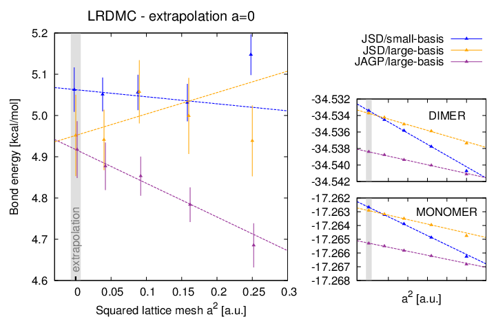
In Tab. 4 we have also reported the results for the LRDMC calculations of the JSD/small-basis1, JSD/large-basis5 and JAGP/large-basis5, and in Fig. 4 we show the dependence on the mesh size of the total energies and of the binding energy. We observe that the evaluation of is 5 kcal/mol for all the three wave functions, in agreement with other highly accurate quantum chemical methods such as the CCSD(T) or the MP2, see Refs. 70, 68. We also observe that the evaluation of seems not affected by the choice of the LRDMC mesh size for the JSD ansatz, at least in the range , whereas a small bias with large can be observed for the JAGP ansatz. Indeed, in Fig. 4 the angular coefficients of the fitting lines for the binding energy is, within the evaluated error of the fitting, compatible with zero for the two JSD calculations, whereas it is not the case for the JAGP wave function. The absolute LRDMC energies for the monomer and the dimer, for the extrapolated , of the JSD/small-basis1 and JSD/large-basis5 ansatzes differ for less than 0.3 mH, indicating that the small-basis1, although much smaller than the large-basis5 and less accurate at the VMC level, provides a nodal surface that seems as good as the one provided by JSD/large-basis5, because the fixed-node projection scheme yields the same electronic correlation for both wave functions.
The evaluations of the total dipole , for the monomer and the dimer, show that these quantities are less affected than by the wave function ansatz, and we have obtained reliable values for all the considered methods. In Fig. 2 we have reported a representation of the electronic density for the dimer, calculated with VMC and with LRDMC(a=0.2). It can be observed that the electrons distribution is very similar in the two methods. Moreover, we observe that, in the region between the donor hydrogen and the acceptor oxygen , the electronic density is always larger than 0.02 a.u. (yellow hypersurface in Fig. 2), due to the presence of the H-bond between the two atoms.

| Method | Ref. | |||||||
|---|---|---|---|---|---|---|---|---|
| BLYP/aug-cc-pVTZ(-f) | Ref. 69 | 2.952 | 5.9 | 0.981 | 0.971 | 0.973 | 104.8 | 104.7 |
| B3LYP/aug-cc-pVTZ(-f) | Ref. 69 | 2.926 | 5.8 | 0.970 | 0.961 | 0.963 | 105.4 | 105.3 |
| CCSD(T)/IO275a | Ref. 70 | 2.912 | 5.5 | 0.964 | 0.957 | 0.958 | 104.8 | 104.9 |
| CCSD(T)/cc-pVQZb | Ref. 67 | 2.910 | 4.8 | 0.964 | 0.957 | 0.959 | 104.3 | 104.6 |
| VMC/JSD/small-basis1c | this work | 2.966 | 3.3 | 0.960 | 0.953 | 0.955 | 104.8 | 105.0 |
| VMC/JSD/large-basis5d | this work | 2.942 | 4.5 | 0.961 | 0.953 | 0.955 | 105.0 | 105.2 |
| Experiment | Ref. 72 | 2.976 0.030 | 620 | |||||
| a IO275: interaction optimized basis set with 275 basis functions for the H2O dimer., see Ref. 70. | ||||||||
| b Structure used in the S22-database [67, 68]. | ||||||||
| c Wave function used for VMC-based MD simulations with 32 and 64 waters in PBC box; see Tab. 2. | ||||||||
| d See Tab. 3 | ||||||||
The JSD/small-basis1 and JSD/large-basis5 wave functions have also been considered for a structural optimization of the water dimer. The results are reported in Tab. 5, and compared with experimental and other ab-initio computational evaluations. The two wave functions provide structures that are very close, indicating that, at a structural level, the smaller basis do not introduce a large bias, at least at the minimum of the potential energy surface. The main difference between them is in the distance between the oxygens, that differs for 0.02 Å. Anyway, both the results are in good agreement with the experimental evaluations and the reported highly accurate quantum chemical calculations.
In order to check our wave function ansatz not only at the structural minimum, but in a larger region of the potential energy surface (PES), we have considered the dissociation of the water dimer. In Fig. 3 we report the total energy (panel a), bond energy (panel b) and total dipole (panel c) of the water dimer in dissociation. The dissociation is realized by considering structures with increasing oxygen-oxygen distance, , in the dimer. At the PES minimum, the donor hydrogen is rotated of a few degrees from the axis connecting the two oxygens, and slightly moved in the direction of the acceptor oxygen with respect to its equilibrium distance in the monomer, see Tab. 5. However, in order to simplify the dissociation plots reported in Fig. 3, we have considered the two water molecules at exactly their equilibrium configuration, and relatively oriented in order to have in the oxygens axis, as in Sterpone et al. [74]. In Fig. 3A we observe that, at the VMC level, each increase in the basis sets here considered leads to an improved variational energy, and also the JAGP ansatz provides a large variational improvement when compared with the JSD calculation on the same basis. As expected, the lower energy is obtained at the LRDMC level, for which we have considered both the JSD/small-basis1 and the JSD/large-basis5 ansatz. The two different trial wave functions appear to yield to the same energies (once the bias for the finite mesh size has been evaluated and corrected), within the stochastic errors of the evaluations. In Fig. 3B we observe that, at the VMC/JSD level, a larger basis gives essentially a vertical shift of the binding energy, at least for not too large distances. This implies that forces should be quite accurate even for the simplest ansatz in the mentioned physical range. This is an important property with respect to the molecular dynamics, that is sensitive only to the accuracy of forces (slope in the binding) and not to the absolute value of the binding energy. Indeed, at the variational level, it appears difficult to define a Jastrow term with a reasonably small number of parameters, that is also able to recover the full dynamical correlation energy, accessible instead at the LRDMC level, providing the correct binding of 5 kcal/mol. As a further evidence of the quality of our variational approach, we observe in Fig. 3C that the dipole, thus the electronic distribution of the charge, is essentially the same for all the considered methods.
A
B C
C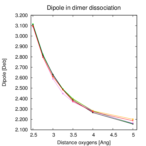
| Method | Dissociation Energy [mH] | ||||
|---|---|---|---|---|---|
| prism | cage | book | ring | ||
| HF | -41.7 | -41.9 ( -0.18 ) | -43.7 ( -2.04 ) | -45.7 ( -3.95 ) | |
| LDA | -123.3 | -123.1 ( 0.17 ) | -121.7 ( 1.63 ) | -117.9 ( 5.37 ) | |
| PBE | -74.8 | -75.2 ( -0.40 ) | -76.5 ( -1.70 ) | -76.0 ( -1.21 ) | |
| PBE0 | -72.0 | -72.3 ( -0.37 ) | -73.5 ( -1.55 ) | -73.4 ( -1.42 ) | |
| BLYP | -60.8 | -61.6 ( -0.76 ) | -64.0 ( -3.16 ) | -64.6 ( -3.78 ) | |
| B3LYP | -65.1 | -65.7 ( -0.58 ) | -67.6 ( -2.44 ) | -68.0 ( -2.87 ) | |
| VMC/JSD/small-basis1 | -56.9 | -56.8 ( 0.06 ) | -56.9 ( -0.09 ) | -55.2 ( 1.67 ) | |
| DMC | Ref. 75 | -73.2 | -72.7 ( 0.53 ) | -72.3 ( 0.90 ) | -70.7 ( 2.45 ) |
| MP2 | Ref. 75 | -73.3 | -73.2 ( 0.09 ) | -72.8 ( 0.46 ) | -71.5 ( 1.81 ) |
| CCSD(T) | Ref. 76 | -76.6 | -76.2 ( 0.46 ) | -74.7 ( 1.92 ) | -73.3 ( 3.33 ) |
| CCSD(T) | Ref. 77 | ( 0.39 ) | ( 1.12 ) | ( 2.70 ) | |
I.4 Choice of the wave function ansatz
Considering that in the VMC-based molecular dynamics we need a stable and compact wave function that can be efficiently, quickly and systematically optimized after every ion movement, and that in the liquid water every water is surrounded by other four waters, with a distance between the oxygens that may range from 2.5Å to 3.5Å, we have chosen the smallest considered basis, i.e. JSD/small-basis1. We are confident that the vertical energy shift observed in the water dimer with larger basis sets or ansatzes with a larger number of parameters, see Fig. 3B, will not affect substantially our results in the liquid water, and that they will be more accurate than the DFT approaches typically used to study the liquid water. Our VMC wave function is indeed a real many-body wave function, which recovers the dynamical electronic correlation with the various terms of the Jastrow factor. We have tested it over the water dimer, in subsection I.3, but we think that the improvement of our VMC approach over DFT, in terms of accuracy, is even larger for liquid water, where the packing of the water molecules makes the correlation larger and more challenging. In support of our believe we show, in Tab. 6, the dissociation energies of four hexamer clusters of waters, respectively in prism, cage, book and ring configuration,[75] calculated with the wave function ansatz and the approach that we have used also for our VMC-based molecular dynamics (VMC with JSD/small-basis1), in comparison with a Hartree-Fock calculation, several DFT calculations with commonly used density functionals, and with some highly accurate quantum chemical approaches: namely diffusion Monte Carlo (DMC), second order Moller-Plesset perturbation theory (MP2), and couple cluster with single, double and perturbative triple excitations (CCSD(T)). In the table we can observe, in agreement with Refs. 75, 77, that the typical DFT approaches rank the four hexamers in the wrong way, in relation to their dissociation energy. The VMC calculations obtained with the ansatz used also for the dynamics is instead much more reliable of any of the DFT-based calculations, and they are in fair agreement with the most accurate calculations.
As already observed, the accuracy of QMC-based calculations are further improved, and indistinguishable from the best known results if the lattice regularized Diffusion Monte Carlo method is applied. However, at present the computer time required for the simulation by LRDMC of several molecules — like the one presented here — is still out of reach. We have to remark that, when considering geometrical relaxation or dynamics, what is important is not the total energy but the forces between couples of atoms, namely it is crucial to have accurate energy derivatives of the binding energy profile. As it can be seen in the inset of Fig. 1, by shifting the binding energy curve in order to have the minimum on the x-axis (the shift not affecting its derivative), we obtain a rather good description of the binding shape in the relevant region of between Å and Å, and an acceptable error in the large distance region. On the other hand, experience has shown that geometrical properties, namely the force values around equilibrium distance, are very well determined by the simple variational ansatz in Eq.(1), as it is clearly shown in Subsection I.3. The LRDMC usually provides only a substantial correction to the energetics, and therefore it is not expected to play an important role for static quantities like .
II Results for Liquid Water
We apply the molecular dynamics driven by quantum Monte Carlo forces (see Methods), introduced recently for the simulation of liquid hydrogen at high pressures[39]. We have employed a simulation of 32 waters in the canonical NVT ensemble at ambient temperature K and experimental density, thus in a cubic cell with box side Å and periodic boundary conditions (PBC). Since the values of the atomic masses are not affecting the static equilibrium properties, we have set both the hydrogen and the oxygen masses to 1 aru, and we have done about 5000 iterations (that we can estimate to roughly correspond to more than 40 ps of simulation in a standard Newtonian MD simulation), where at each iteration we optimize about 12000 variational parameters with 9 steps of efficient energy optimizations based on the so called linear method[78]. We have done several tests[38] confirming that it is possible with this scheme to correctly follow the Born-Oppenheimer energy surface, namely the variational wave function remains at the minimum possible energy during the time evolution of the atomic positions. The RDFs that we obtain from the VMC-based molecular simulations, having neglected the first 2000 steps of equilibration, are reported in Fig. 5, in comparison with experimental results. We have verified that, within this Langevin scheme, the correlation time estimated by the convergence of the RDF is less than 2000 iterations, and therefore we are confident that our results represent well equilibrated properties. At variance of the Newtonian dynamics, our advanced method makes use of an appropriate friction matrix, which has been proved to be very helpful to reduce the autocorrelation time[38] as it allows a smooth approach to the equilibrium (see Fig. 6).

A blow-up of the oxygen-oxygen first peak is reported in Fig. 6.

As a starting point of our dynamics we have used equilibrated configurations generated by the DFT molecular dynamics with BLYP functional. The BLYP functional describes the water dimer (the simplest system displaying the hydrogen bond) with a reasonable accuracy, comparable with the one obtained within our VMC scheme, as can be seen in Fig. 1. Nevertheless, the peak positions and shapes of the RDFs are substantially different on the target 32 water system.
We see in Fig. 5 that these first results are very encouraging. Despite the noise, the outcome is quite clear, because the is much closer to experiments than the corresponding DFT calculations. Not only the radial distribution function is much less overstructured but also, as discussed in the introduction, the position of the first peak is almost indistinguishable from the most recent experiments [33, 34]. At this point it is worth to comment about the error bars in the experimental data. While the Skinner data are extracted from the x-ray scattering intensities, the Soper data[35, 79, 34] are obtained from Empirical Potential Structural Refinement (EPSR) of joint neutron and x-ray data, i.e. they are not bare neutron diffraction data. The large error bars of Soper (2000) are therefore not directly experimental error bars but they refer to a range of different EPSR fits that would model almost equally well the experimental data. Better fits have been published by the same author more recently, see e.g. Ref. 34, which reports the likely best structural refinement to date. From the theoretical side the quality of the approximation used for the electronic correlation affects the accuracy of the RDFs profile. In fact, the first peak’s position has been already improved with respect to standard DFT functionals by employing the simplest (MP2) post-Hatree-Fock technique[80]. Moreover quantum effects should broaden the peaks without shifting the corresponding maxima, as it was shown before, within DFT, in Ref. 27. Although this remains, until now, a rather controversial issue[32, 81], because of the lack of long enough ab-initio simulations with quantum effects included, our results seem to support the claim made in Ref. [27] about the relevance of proton quantum corrections in water. Indeed our RDFs for classical ions remain sizably different from experiments, as far as the broadening and the heights of the first peaks are concerned, especially for what concerns the and radial distribution functions, where quantum effects are expected to be much more important. In addition, quantum effects also enhance the the probability of the transient autoprotolysis events, namely proton transfer between water molecules, which were found in a small but nonnegligible fraction by measuring the proton-transfer coordinate[32]. Consistently, during our classical-ions simulation with VMC, the autoprotolysis event has not been observed, see Fig. 7.
In order to avoid possible size effects we have studied in Fig. 6 the position of the first peak with a much shorter simulation (600 steps, corresponding to about 5ps) with 64 molecules. Our method equilibrates rather smoothly with the length of the simulation (say, ), and this nice property, coming from our optimized damped MD, has allowed us to obtain a rather well converged value of the peak position also in the 64 water case. This further supports the validity of our claim.
III Discussion and Conclusion
In conclusion, we have done the first ab-initio simulation of liquid water by quantum Monte Carlo, showing that this technique is now mature to enter the field of ab initio molecular simulations. This opens a new frontier in water simulations, because several questions about its structure, its electronic properties and the phase diagram, also difficult to answer experimentally, can be tackled in the near future thanks to the usage of massive parallel supercomputers and quantum Monte Carlo methods. We have adopted the most simple quantum Monte Carlo method (the VMC) in a fully consistent and controlled way. Despite the roughness of this first attempt (as compared with the most recent DFT calculations), a few clear results come out from our study:
- •
The calculation by QMC is feasible albeit computationally heavy, and there is room for considerable improvements along this fully ab-initio scheme. For instance it could be possible to work with a larger but more accurate basis (see Fig. 3 and Tab. 4) with at most a factor ten more computer resources, as our algorithm scales quadratically with the basis dimension. Moreover, even larger improvements in the QMC-based accuracy are expected when moving from the variational scheme, adopted in this work, to fixed-node projection schemes. Fig. 4 shows how both the small and large basis provides a binding energy for the water dimer, evaluated via LRDMC, that are statistically in agreement with highly accurate benchmarks[68, 70] coming from CCSD(T) (5.02 kcal/mol). Thus, the most convenient choice is given by the smallest basis, allowing a much cheaper wavefunction optimization during the dynamics, and in principle also an efficient evaluation of the fixed-node diffusion forces for every new nuclear configuration. However, the DMC is also affected by the finite time step error (in the case of ordinary DMC) or the finite lattice mesh (in the case of the LRDMC scheme used here), and the solution of the infinite variance problem in DMC (or LRDMC) has not been clearly solved yet. Therefore we expect that the computational cost for this DMC-based molecular dynamics would be easily two order or magnitude larger than the VMC based method proposed here.
- •
The simulated structural properties of liquid water, obtained within our VMC-based molecular dynamics, appears much closer to the experimental observations when compared with DFT-based molecular dynamics simulations, at least within standard GGA functionals, such as BLYP and PBE. This is remarkable, because, within our approximation, the two-water interaction was basically dealt with the same degree of accuracy of the BLYP functional. As discussed in subsection I.4, this implies that the accurate description of the many water energy surface, and probably the long distance interactions — usually described within DFT by ”ad hoc” strategies — should be important to close the gap with experiments. In this respect, and in order to support our claim on much simpler systems, we have also verified that our simple variational wave function provides a satisfactory description of water hexamers, in good agreement with the most accurate quantum chemical approaches[75, 77] — MP2, DMC, CCSD(T) — and in contrast with most current DFT functionals for liquid water (see Tab. 6). In order to put further evidence about the systematic difference between QMC and DFT with BLYP functional we show in Fig. 8 that the interaction between two water monomers, namely the repulsive force acting on the O-O axis, is much different from the BLYP prediction when they are in the liquid water and not in the vacuum.
- •
It is clear that our work can help the DFT community to define accurate but also consistent functionals, able to reproduce the experimental results, together with a good description of the chemical interactions between water molecules.
- •
Our agreement with experiment is rather satisfactory, and could be probably improved if the a larger system (64 waters could be sufficient) and nuclear quantum corrections (not included in this study) would be considered. Indeed the height of the first peak is expected to be overestimated by [11, 5] with respect to the converged value in a DFT dynamics with 32 waters. If we assume that also in QMC we have the same effects, the agreement with the experimental value should be substantially improved. Moreover, the inclusion of nuclear quantum effects appears to reduce further the height of the first peak by about () if we consider as reference the path integral CPMD calculation reported in Ref. 27 (Ref. 81). Therefore, in future studies, by taking into account both size effects and the effect of quantum nuclei, it may be possible to have a fully consistent ab-initio description of liquid water by QMC.
We finally remark that, thanks to good scaling properties of QMC algorithms with the system size, this work opens promising perspectives for future applications of such high-level ab initio molecular dynamics technique to study the finite temperature properties of complex liquids and materials.


Acknowledgements.
A.Z and L.G. acknowledge fundings provided by the European Research Council project n. 240624 within the VII Framework Program of the European Union. Computational resources were supplied by CINECA, PRACE infrastructure (Project 2013081585), the Caliban-HPC centre at the University of L’Aquila and the K-computer at AICS Riken. G.M acknowledges T. Kühne and J. Vandevondele, and A.Z. acknowledges A. Michaelides and R. Potestio for useful discussions.References
- [1] R. Car and M. Parrinello, Phys. Rev. Lett. 55, 2471 (1985).
- [2] K. Laasonen, M. Sprik, M. Parrinello, and R. Car, J. Chem. Phys. 99, 9080 (1993).
- [3] M. Sprik, J. Hutter, and M. Parrinello, J. Chem. Phys. 105, 1142 (1996).
- [4] Z. Ma, Y. Zhang, and M. E. Tuckerman, J. Chem. Phys. 137, 044506 (2012).
- [5] T. D. Kühne, M. Krack, and M. Parrinello, J. Chem. Theory Comput. 5, 235 (2009).
- [6] P. H. L. Sit and N. Marzari, J. Chem. Phys. 122, 204510 (2005).
- [7] S. Yoo, X. C. Zeng, and S. S. Xantheas, J. Chem. Phys. 130, 221102 (2009).
- [8] J. VandeVondele, F. Mohamed, M. Krack, J. Hutter, M. Sprik, and M. Parrinello, J. Chem. Phys. 122, 014515 (2005).
- [9] H.-S. Lee and M. E. Tuckerman, J. Chem. Phys. 125, 154507 (2006).
- [10] H.-S. Lee and M. E. Tuckerman, J. Chem. Phys. 126, 164501 (2007).
- [11] J. C. Grossman, E. Schwegler, E. W. Draeger, F. Gygi, and G. Galli, J. Chem. Phys. 120, 300 (2004).
- [12] I. Kuo, C. Mundy, M. McGrath, J. Siepmann, J. VandeVondele, M. Sprik, J. Hutter, B. Chen, M. Klein, F. Mohamed, et al., J. Phys. Chem. B 108, 12990 (2004).
- [13] T. Todorova, A. P. Seitsonen, J. Hutter, I.-F. W. Kuo, and C. J. Mundy, J. Phys. Chem. B 110, 3685 (2006).
- [14] M. Guidon, F. Schiffmann, J. Hutter, and J. VandeVondele, J. Chem. Phys. 128, 214104 (2008).
- [15] C. Zhang, D. Donadio, F. Gygi, and G. Galli, J Chem. Theory Comput. 7, 1443 (2011a).
- [16] R. A. DiStasio, Jr., B. Santra, Z. Li, X. Wu, and R. Car, J. Chem. Phys. 141, 084502 (2014).
- [17] S. Grimme, J. Comput. Chem. 25, 1463 (2004).
- [18] S. Grimme, J. Comput. Chem. 27, 1787 (2006).
- [19] O. von Lilienfeld, I. Tavernelli, U. Rothlisberger, and D. Sebastiani, Phys. Rev. Lett. 93, 153004 (2004).
- [20] M. Dion, H. Rydberg, E. Schröder, D. C. Langreth, and B. I. Lundqvist, Phys. Rev. Lett. 92, 246401 (2004).
- [21] J. Schmidt, J. VandeVondele, I. F. W. Kuo, D. Sebastiani, J. I. Siepmann, J. Hutter, and C. J. Mundy, J. Phys. Chem. B 113, 11959 (2009).
- [22] I.-C. Lin, A. P. Seitsonen, M. D. Coutinho-Neto, I. Tavernelli, and U. Rothlisberger, J. Phys. Chem. B 113, 1127 (2009).
- [23] I.-C. Lin, A. P. Seitsonen, I. Tavernelli, and U. Rothlisberger, J. Chem. Theory Comput. 8, 3902 (2012).
- [24] J. Wang, G. Román-Pérez, J. M. Soler, E. Artacho, and M. V. Fernández-Serra, J. Chem. Phys. 134, 024516 (2011).
- [25] C. Zhang, J. Wu, G. Galli, and F. Gygi, J. Chem. Theory Comput. 7, 3054 (2011b).
- [26] M. A. Morales, J. R. Gergely, J. McMinis, J. M. McMahon, J. Kim, and D. M. Ceperley, J. Chem. Theory Comput. p. 140512175104006 (2014).
- [27] J. Morrone and R. Car, Phys. Rev. Lett. 101, 017801 (2008).
- [28] S. Habershon, T. E. Markland, and D. E. Manolopoulos, J. Chem. Phys. 131, 024501 (2009).
- [29] F. Paesani and G. A. Voth, J. Phys. Chem. B 113, 5702 (2009).
- [30] F. Paesani, S. Yoo, H. J. Bakker, and S. S. Xantheas, J. Phys. Chem. Lett. 1, 2316 (2010).
- [31] X. Z. Li, B. Walker, and A. Michaelides, Proc. Natl. Acad. Sci. U. S. A. 108, 6369 (2011).
- [32] M. Ceriotti, J. Cuny, M. Parrinello, and D. E. Manolopoulos, Proc. Natl. Acad. Sci. U. S. A. 110, 15591 (2013).
- [33] L. B. Skinner, C. Huang, D. Schlesinger, L. G. M. Pettersson, A. Nilsson, and C. J. Benmore, J. Chem. Phys. 138, 074506 (2013).
- [34] A. K. Soper, ISRN Phys. Chem. 2013, 1 (2013).
- [35] A. K. Soper, Chem. Phys. 258, 121 (2000).
- [36] E. Coccia, D. Varsano, and L. Guidoni, J. Chem. Theory Comput. p. 140114080315003 (2014).
- [37] A. Zen, D. Zhelyazov, and L. Guidoni, J. Chem. Theory Comput. 8, 4204 (2012).
- [38] Y. Luo, A. Zen, and S. Sorella, J. Chem. Phys. 141, 194112 (2014).
- [39] G. Mazzola, S. Yunoki, and S. Sorella, Nat. Commun. 5, 3487 (2014).
- [40] G. Mazzola and S. Sorella, Phys. Rev. Lett. 114, 105701 (2015).
- [41] W. M. C. Foulkes, L. Mitas, R. J. Needs, and G. Rajagopal, Rev. Mod. Phys. 73, 33 (2001).
- [42] J. Grossman and L. Mitas, Phys. Rev. Lett. 94, 056403 (2005).
- [43] C. Attaccalite and S. Sorella, Phys. Rev. Lett. 100, 114501 (2008).
- [44] G. Mazzola, A. Zen, and S. Sorella, J. Chem. Phys. 137, 134112 (2012), ISSN 0021-9606, 1089-7690.
- [45] F. A. Reboredo and J. Kim, J. Chem. Phys. 140, 074103 (2014).
- [46] D. M. Ceperley and M. Dewing, The Journal of Chemical Physics 110, 9812 (1999), ISSN 0021-9606, 1089-7690.
- [47] See s. sorella’s talk at the “advances in quantum monte carlo techniques for non-relativistic many-body systems”, http://www.int.washington.edu/talks/WorkShops/int_13_2a/ (June 27, 2013).
- [48] T. Kühne, M. Krack, F. Mohamed, and M. Parrinello, Phys. Rev. Lett. 98, 066401 (2007).
- [49] E. Schwegler, J. C. Grossman, F. Gygi, and G. Galli, J. Chem. Phys. 121, 5400 (2004).
- [50] N. D. Drummond, M. D. Towler, and R. J. Needs, Phys. Rev. B 70, 235119 (2004).
- [51] A. Zen, Y. Luo, S. Sorella, and L. Guidoni, J. Chem. Theory Comput. 9, 4332 (2013).
- [52] M. Casula, C. Filippi, and S. Sorella, Phys. Rev. Lett. 95, 100201 (2005).
- [53] M. Casula, S. Moroni, S. Sorella, and C. Filippi, J. Chem. Phys. 132, 154113 (2010).
- [54] M. Marchi, S. Azadi, M. Casula, and S. Sorella, J. Chem. Phys. 131, 154116 (2009).
- [55] S. Sorella, TurboRVB quantum monte carlo package (accessed date may 2013), URL http://people.sissa.it/~sorella/web/index.html.
- [56] C. Attaccalite, Ph.D. thesis, SISSA of Trieste (2005).
- [57] S. Sorella, M. Casula, L. Spanu, and A. Dal Corso, Phys. Rev. B 83, 075119 (2011).
- [58] F. R. Petruzielo, J. Toulouse, and C. J. Umrigar, J. Chem. Phys. 134, 064104 (2011).
- [59] M. Casula and S. Sorella, J. Chem. Phys. 119, 6500 (2003).
- [60] S. Sorella, M. Casula, and D. Rocca, J. Chem. Phys. 127, 014105 (2007).
- [61] M. Burkatzki, C. Filippi, and M. Dolg, J. Chem. Phys. 126, 234105 (2007).
- [62] B. Braïda, J. Toulouse, M. Caffarel, and C. J. Umrigar, J. Chem. Phys. 134, 084108 (2011).
- [63] A. G. Anderson and W. A. Goddard, J. Chem. Phys. 132, 164110 (2010).
- [64] P. M. Zimmerman, J. Toulouse, Z. Zhang, C. B. Musgrave, and C. J. Umrigar, J. Chem. Phys. 131, 124103 (2009).
- [65] A. Zen, E. Coccia, Y. Luo, S. Sorella, and L. Guidoni, J. Chem. Theory Comput. 10, 1048 (2014).
- [66] A. Zen, E. Coccia, S. Gozem, M. Olivucci, and L. Guidoni, J. Chem. Theory Comput. 0, null (2015), URL http://dx.doi.org/10.1021/ct501122z.
- [67] P. Jurecka, J. Sponer, J. Cerny, and P. Hobza, Phys. Chem. Chem. Phys. 8, 1985 (2006).
- [68] S22-benchmark noncovalent complexes, URL http://www.begdb.com/index.php?action=oneDataset&id=4&state=show&order=ASC&by=name_m&method=.
- [69] X. Xu and W. A. Goddard, J. Phys. Chem. A 108, 2305 (2004).
- [70] W. Klopper, J. G. C. M van Duijneveldt-van de Rijdt, and F. B. van Duijneveldt, Phys. Chem. Chem. Phys. 2, 2227 (2000).
- [71] S. A. Clough, Y. Beers, G. P. Klein, and L. S. Rothman, J. Chem. Phys. 59, 2254 (1973).
- [72] J. A. Odutola and T. R. Dyke, J. Chem. Phys. 72, 5062 (1980).
- [73] E. Neuscamman, Phys. Rev. Lett. 109, 203001 (2012).
- [74] F. Sterpone, L. Spanu, L. Ferraro, S. Sorella, and L. Guidoni, J. Chem. Theory Comput. 4, 1428 (2008).
- [75] B. Santra, A. Michaelides, M. Fuchs, A. Tkatchenko, C. Filippi, and M. Scheffler, J. Chem. Phys. 129, 194111 (2008).
- [76] R. M. Olson, J. L. Bentz, R. A. Kendall, M. W. Schmidt, and M. S. Gordon, J. Chem. Theory Comput. 3, 1312 (2007).
- [77] M. J. Gillan, F. R. Manby, M. D. Towler, and D. Alfe, J. Chem. Phys. 136, 244105 (2012).
- [78] C. J. Umrigar, J. Toulouse, C. Filippi, S. Sorella, and H. Rhenning, Phys. Rev. Lett 98, 110201 (2007).
- [79] A. Soper and B. C.J., Phys. Rev. Lett. 101, 065502 (2008).
- [80] M. Del Ben, M. Schönherr, J. Hutter, and J. VandeVondele, J. Phys. Chem. Lett. 4, 3753 (2013).
- [81] S. Fritsch, R. Potestio, D. Donadio, and K. Kremer, J. Chem. Theory Comput. p. 140123151236004 (2014).