Trapping reaction in a symmetric double well potential

Trilochan Bagarti ^†^†thanks: bagarti@hri.res.in Affiliation: Harish-Chandra Research Institute
Chhatnag Road,Jhunsi, Allahabad-211019 Kalyan Kundu Affiliation: Institute of Physics
Sachivalaya Marg, Bhubaneswar-751005

Abstract

We study the trapping reaction-diffusion problem in a symmetric double well potential in one dimension with a static trap located at the middle of the central barrier of the double well. The effect of competition between the confinement and the trapping process on the time evolution of the survival probability is considered. The solution for the survival probability of a particle is obtained by the method of Green’s function. Furthermore, we study trapping in the presence of a growth term. We show that for a given growth rate there exist a threshold trapping rate beyond which the population can become extinct asymptotically. Numerical simulations for a symmetric quartic potential are done and results are discussed. This model can be applied to study the dynamics of a population in habitats with a localized predation.

1 Introduction

The trapping reaction diffusion model is one of the simplest models of diffusion limited reaction process. It has been used to describe a wide variety of phenomena such as the trapping of excitons in crystals, recombination of electron and hole, formation of soliton-antisoliton pair, reaction activated by catalysis[1]. The trapping reaction diffusion process consists of (i) free diffusion of a particle $A$ and (ii) the absorption of a particle whenever it encounters a trap $T$ . The trapping reaction $A+T\rightarrow T$ shows anomalous kinetics that depends on the spatial dimension. For the simplest case of a single trap, the number of particles $n(t)$ decay as $t^{-1/2}$ in one dimensional space $d=1$ and $1/\log t$ when $d=2$ [2].

The trapping problem with multiple traps randomly distributed in space has also been studied intensively in the past. In the asymptotic time limit it has been shown that, for static traps, $n(t)$ decays as a stretched exponential $\exp(-\alpha_{d}\rho^{2/(2+d)}t^{d/(2+d)})$ , where $\alpha_{d}$ is a constant that depends on the spatial dimension $d$ and $\rho$ is the mean density of traps[3, 4, 5]. The stretched exponential behavior appears due to large trap free regions where particles can spend exponentially long time before they get absorbed at a trap[5]. Trapping reaction can induce self-segregation of the reactant species[6, 7], self-organization around traps[8, 9, 10, 11]. In the presence of volume exclusion it has been found that, an additional term appears in the stretched exponent which effectively slightly increases (decreases) the trapping rate[12, 13]. Similar anomalous behavior is observed in quantum transport in the presence of traps. However it has been found that the stretched exponential behavior in the quantum regime is slower than its diffusive counterpart[14, 15, 16, 17]. Random multiplication of particles in a diffusive medium which models chemical reactions, evolution of biological species, etc have been studied[18, 19, 20]. For a population which undergoes multiplication and decay at random positions in space, it has been shown by using the knowledge of density of state for disordered system, that the asymptotically $n(t)$ is exponential times the survival probability for the single trap trapping problem.

Recently, trapping of a diffusing particle in a harmonic potential has been studied with the trap located at various position relative to the bottom of the potential and the initial position of the particle[21]. This model was motivated by problems in biophysics such as photosynthesis, DNA stretching with optical tweezers, etc. Trapping problem with a potential can also be studied in the quantum regime.

In this paper we study the trapping reaction-diffusion model with an external confining potential. We consider a symmetric double well potential and a trap at the origin. Our motivation in this work comes from possible applications in ecology. We shall briefly discuss the scenario in Sec. 2 where we describe the reaction diffusion model. In Sec. 3, we study by using Green’s function technique, the trapping of a single particle in a square double well potential. Trapping with growth has been studied in Sec. 4 and the competition between decay and growth is discussed. Finally, numerical results for a general quartic double well potential has been discussed in Sec. 5.

2 Reaction-diffusion equations

We consider particles diffusing in the presence of a external confining potential $V(x)$ with a trap located at the origin. We assume a symmetric double well potential with a maximum at the origin. When a particle encounters the trap during its motion it gets absorbed at a rate $\kappa$ . Let us denote by $u(x,t)$ the density of particles at position $x$ at time $t$ . The reaction-diffusion equation can be written as

\displaystyle\partial_{t}u=D\partial_{x}^{2}u-\partial_{x}(\phi u)-\kappa\delta(x)u+F(u),

(1)

where $D$ is the diffusion coefficient of the particle, $\phi(x):=-\bar{\gamma}^{-1}\partial_{x}V(x)$ with $-\partial_{x}V(x)$ being the force on the diffusing particle due to the potential and $\bar{\gamma}$ is damping constant such that $D=k_{B}T/\bar{\gamma}$ . The term $-\kappa\delta(x)u$ describes the trapping reaction at the origin and $F(u)$ describes the growth of the population. The boundary condition is $\lim_{|x|\rightarrow\infty}u(x,t)=0$ and the initial condition is $u(x,0)=f(x)$ .

Application to ecology: This simple model can be applied to a two species predator-prey model with a localized predation. The external potential can be used to model the habitats. A typical example could be the predator-prey dynamics of herbivore and crocodile, fishing by humans etc. The predator in these cases are localized in a small region where as the prey can diffuse from one habitat to other. The knowledge of the predator localized at some region can build a fear in the prey. This will create a barrier that gives rise to repulsion away from the predation region. A part of the potential can also arise from basic problems of accessibility between two habitats. Two villages connected by bad roads or by turbulent rivers can be an example. The tendency of the prey to stay in herds can be incorporated by an attraction towards the center of the herd. The size of the herd may depend on the size of the habitat. These two effects can naturally be incorporated by a double well potential in the reaction-diffusion equation.

3 Trapping of a single particle

The trapping of a single particle in the presence of an external potential can be considered as an inhomogeneous pure death process, $F(u)=0$ . Let us consider a square double well potential with a barrier height $V_{0}$ (see Fig. 1) with a particle located initially in right well at $x=a$ . Using the transformation $t\rightarrow Dt,~V\rightarrow$ $~V/k_{B}T,~\kappa\rightarrow\kappa/D,~$ in Eq. (1) we obtain

\partial_{t}u=\partial_{x}^{2}u-\partial_{x}(\phi u)-\kappa\delta(x)u.

(2)

Note that due to the said transformations, in Eq. (2), $V(x)$ is dimensionless and consequently $\phi=-\partial_{x}V(x)$ has the dimension of length . Furthermore $t$ has the dimension of (length)² and $\kappa$ has the dimension of inverse length. We gain note that the Laplace Transform of Eq. (2) can be solved exactly by the method of Green’s function. Let $\tilde{u}(x,s)$ be the Laplace transform of the the density $u(x,t)$ so that we have

\left[s-\partial_{x}^{2}+\partial_{x}\phi\right]\tilde{u}(x,s)=u(x,0)-\kappa\delta(x)\tilde{u}(x,s).

(3)

The solution $\tilde{u}(x,s)$ can be written as

\tilde{u}(x,s)=G(x|a)-\frac{\kappa G(x|0)G(0|a)}{1+\kappa G(0|0)},

(4)

where $G=\left[s-\partial_{x}^{2}-\partial_{x}\phi\right]^{-1}$ is the Green’s operator in the coordinate representation (see Appendix A).

Refer to caption — Figure 1: Symmetric square double well potential.

3.1 Survival probability

The survival probability $S(t)$ is defined as

\displaystyle S(t)

\displaystyle=\int u(x,t)dx.

(5)

From Eq. (4) we obtain

\tilde{S}(s)=\frac{1}{q^{2}}-\frac{\kappa G(0|a)}{zq^{2}(1+\kappa G(0|0))},

(6)

where

	$\displaystyle G(0\|0)$	$\displaystyle=\frac{\cosh(Lq)\cosh(\alpha q)+\sinh(Lq)\sinh(\alpha q)z}{2qz(\cosh(Lq)\sinh(\alpha q)+\sinh(Lq)\cosh(\alpha q)z)},$
	$\displaystyle G(0\|a)$	$\displaystyle=\frac{\cosh(q(L+\alpha-a))}{2q(\cosh(Lq)\sinh(\alpha q)+\sinh(Lq)\cosh(\alpha q)z)},$		(7)

$z=\exp(V_{0})$ , $L=\beta-\alpha$ and $q=\sqrt{s}$ . We first compute the survival probability $S_{0}(t)$ for the case where the width of the wells is large, i.e. $\lim L\rightarrow\infty$ limit. For this case the finite width of the barrier is of no consequence. So we assume that $\alpha\rightarrow 0$ . The expression in Eq. (6) becomes

\tilde{S}(s)=\frac{1}{q^{2}}-\frac{\kappa~\mbox{e}^{-qa}}{z^{2}q^{2}(\kappa/z^{2}+2q)},

(8)

The Inverse Laplace transform of Eq. (8) gives the survival probability

S_{0}(t)=1-\mbox{erfc}\left(\frac{a}{2\sqrt{t}}\right)+\exp\left(\frac{a\tilde{\kappa}}{2}+\frac{\tilde{\kappa}^{2}t}{4}\right)\mbox{erfc}\left(\frac{a}{2\sqrt{t}}+\frac{\tilde{\kappa}\sqrt{t}}{2}\right),

(9)

where $\tilde{\kappa}=\kappa/z^{2}$ . This result can also be obtained from Eq. (6) by substituting for the Green’s function, $G(x|y)=\exp(-q|x-y|)/2q$ and setting the trapping rate $\kappa\rightarrow\kappa/z^{2}$ . The result Eq. (9) is well known and it is the survival probability of a particle which is initially at position $x=a$ and diffuses to get trapped at the origin[22].

The survival probability $S(t)$ for the general case can be obtained by computing the Inverse Laplace Transform of Eq. (6). The first term $1/q^{2}$ yields $1$ . Substituting $q=\sqrt{s}$ in Eq. (6), the inverse Laplace transform of the second term can be written as

\frac{1}{2\pi i}\int^{\gamma+i\infty}_{\gamma-i\infty}\frac{G(0|a)\mbox{e}^{st}ds}{s(1+\kappa G(0|0))}=\frac{1}{2\pi i}\int^{\gamma+i\infty}_{\gamma-i\infty}\frac{\cosh(\sqrt{s}(L+\alpha-a))\mbox{e}^{st}ds}{s(A(s)+\kappa^{\prime}B(s))},

(10)

where $\kappa^{\prime}=\kappa/z$ , $A(s)=2\sqrt{s}~[\cosh(L\sqrt{s})\sinh(\alpha\sqrt{s})+z\sinh(L\sqrt{s}))\cosh(\alpha\sqrt{s})]$ ,
$B(s)=\cosh(L\sqrt{s})\cosh(\alpha\sqrt{s})+z\sinh(L\sqrt{s})\sinh(\alpha\sqrt{s})$ . The poles of the integrand in Eq. (10) are $s=0$ and the zeros of $A(s)+\kappa^{\prime}B(s)$ . The zeros $s^{*}$ satisfy

\cos(L\rho)(\kappa^{\prime}\cos(\alpha\rho)-2\rho\sin(\alpha\rho))-z\sin(L\rho)(\kappa^{\prime}\sin(\alpha\rho)+2\rho\cos(\alpha\rho))=0,

(11)

where $\rho=\sqrt{|s^{*}|}$ .

For the case $\kappa=0$ , the denominator of the integrand in Eq. (10) becomes $sA(s)$ . Although the integral for this case can be evaluated, one observes from Eq. (6) that its contribution to the survival probability shall be zero. Therefore, for $\kappa=0$ , $S(t)=1$ for all $t>0$ .

For $\kappa\neq 0$ , the residue at $s=s^{*}\neq 0$ is $2\pi i\cosh(\sqrt{s^{*}}(L+\alpha-a))\exp(s^{*}t)/[s^{*}\partial_{s}(A(s^{*})+\kappa^{\prime}B(s^{*}))]$ . For $s=0$ , the residue is $2\pi i/\kappa^{\prime}$ . Using Eq. (6) in Eq. (10) the expressions for the survival probability becomes

S(t)=\frac{\kappa}{z}\sum_{\rho}\frac{\cos(\rho(L+\alpha-a))}{F(\rho)}\mbox{e}^{-\rho^{2}t},

(12)

where $F(\rho)=s^{*}\partial_{s}(A(s^{*})+\kappa^{\prime}B(s^{*}))|_{s^{*}=-\rho^{2}}$ . The values of $\rho$ can be computed using Eq. (11).

In Fig. 2(a) we plot survival probability $S(t)$ as a function of time. For small values of the well width (i.e. $L\sim\alpha$ ) we note that it decays exponentially (inset (b) where $\log S(t)$ has a linear behavior). However, for large well width $L\gg\alpha$ the survival probability $S(t)$ deviates from a single exponential decay as seen in Fig. 2. The explanation is as follows. With the range of time, $t$ keeping fixed, when the length of the well is increased, contributions start coming not only from the lowest eigenvalue, but also from other near by eigenvalues. So, there will be a deviation from a single exponential behavior as seen in this calculation. This we have already seen in Eq. (9) for the limiting case $L\rightarrow\infty$ (see inset Fig. 2(c)). In the limit $L\rightarrow\infty$ , eigenvalues form a quasi-continuum spectra and the limiting behavior is obtained by integrating over the spectral region. Furthermore, the survival probability at long time decays monotonically as a function of trapping rate $\kappa$ for all $L$ with the rate of decay smaller for larger $L$ (see Fig. 3). This is due to the fact that a particle has the probability of moving away from a trap for a long time consequently reducing the over all decay probability.

3.2 Short time behavior

To calculate the survival probability at small time we need to expand the Green’s function at large values of $q$ or $s$ . The Green’s function for large $q$ can be written as

G(x|y)\simeq\frac{\mbox{e}^{-q|x-y|}}{q}\left\{\begin{array}[]{ll}1/2z&\mbox{~~~if~~~}|x|<\alpha,|y|<\alpha,\\ 1/(1+z)&\mbox{~~~if~~~}|x|<\alpha,|y|>\alpha,\\ 1/(1+z)&\mbox{~~~if~~~}|x|>\alpha,|y|<\alpha,\\ 1/2&\mbox{~~~if~~~}|x|>\alpha,|y|>\alpha,\\ \end{array}\right.

(13)

Substituting in Eq. (6) we obtain

\tilde{S}(s)=\frac{1}{q^{2}}-\frac{\kappa~\mbox{e}^{-qa}}{z(1+z)q^{2}(\kappa/2z+q)},

(14)

The Inverse Laplace Transform yields

S(t)\simeq 1-\frac{2}{1+z}\left\{\mbox{erfc}\left(\frac{a}{2\sqrt{t}}\right)-\exp\left(\frac{\kappa a}{2z}+\frac{\kappa^{2}t}{4z^{2}}\right)\mbox{erfc}\left(\frac{a}{2\sqrt{t}}+\frac{\kappa\sqrt{t}}{2z}\right)\right\}.

(15)

We note that the survival probability of a particle depends only on the scaled barrier height $V_{0}$ , the trapping rate $\kappa$ and the distance from the the initial position to the trap $a$ . The effect of confinement can be seen in the asymptotic time limit. Near $t=0$ , $S(t)$ can be written as

S(t)\simeq 1-\frac{4\kappa}{\sqrt{\pi}a^{2}(1+z)z}t^{3/2}\mbox{e}^{-a^{2}/4t}.

(16)

3.3 Long time behavior

In the limit $L\rightarrow\infty$ and in the asymptotic time limit $t\rightarrow\infty$ the survival probability for the limiting case Eq. (9) shows a power law decay. Expanding $S_{0}(t)$ for large values of $t$ we obtain

S_{0}(t)\sim\frac{1}{\sqrt{\pi}}\left(a+\frac{2}{\tilde{\kappa}}\right)t^{-1/2}.

(17)

Let us now consider the general case where $L$ is finite. Near $s=0$ we have

	$\displaystyle G(0\|0)$	$\displaystyle\sim\frac{1-(L^{2}+\alpha^{2}-2zL\alpha)s/2)}{2sz[\alpha+Lz-\alpha L(\alpha z+L)s/2]}$
	$\displaystyle G(0\|a)$	$\displaystyle\sim\frac{1+(L+\alpha-a)^{2}s}{2s[\alpha+Lz-\alpha L(\alpha z+L)s/2]}.$		(18)

Substituting Eq. (18) expression in Eq. (6) we obtain the asymptotic survival probability

S(t)\simeq\left(1-\frac{\kappa^{\prime}(L+\alpha-a)^{2}}{4(\alpha+Lz)+\kappa^{\prime}(L^{2}+\alpha^{2}+2\alpha Lz)}\right)\exp({\frac{-\kappa^{\prime}t}{2(\alpha+Lz)+\kappa^{\prime}(L^{2}+\alpha^{2}+2\alpha Lz)/2}}).

(19)

4 Trapping reaction for a growing population

For a vanishing growth term in Eq. (1) particles eventually get trapped as they cannot escape the confining potential. Therefore, we cannot have a nonzero population surviving in the asymptotic large time limit. However, with a nonzero growth i.e. for a predator-prey system, the population may sustain itself in the asymptotically large time regime. It would be interesting to find a threshold predation rate $\kappa=\kappa_{c}$ above which the population may lead towards extinction.

4.1 Trapping with linear growth

Let us consider the case of linear growth

\partial_{t}u=\partial_{x}^{2}u-\partial_{x}(\phi u)-\kappa\delta(x)u+\lambda u.

(20)

It can be shown that Eq. (20) can be reduced to that of the trapping of a single particle with density $u^{\prime}(x,t)=u(x,t)\exp(-\lambda t)$ . As a result the total population $N(t)=\int u(x,t)dx$ can be written as the product of the survival probability $S(t)$ and $\exp(\lambda t)$ .

In the limiting case we have $N(t)=S_{0}(t)\exp(\lambda t)$ . Using Eq. () the asymptotic population can be written as

\lim_{t\rightarrow\infty}N(t)=:N_{\infty}(t)\simeq\frac{1}{\sqrt{\pi}}\left(a+\frac{2}{\tilde{\kappa}}\right)t^{-1/2}\exp(\lambda t).

(21)

Clearly, the population diverges for all $\tilde{\kappa}>0$ . Hence, there exist no threshold $\kappa_{c}$ for a linear growth model in the limiting case $L\rightarrow\infty$ . In other words, for a large habitat size, localized predation cannot drive a linearly growing population extinct.

Similarly, for $L$ finite using Eq. (19) we have

N_{\infty}(t)\sim\exp({\frac{-\kappa^{\prime}t}{2(\alpha+Lz)+\kappa^{\prime}(L^{2}+\alpha^{2}+2\alpha Lz)/2}}+\lambda t).

(22)

We observe from Eq. (22) that there exist a threshold rate $\kappa^{\prime}=\kappa_{c}$ above which the population becomes extinct(see Fig. 4). Note that if $\lambda>2/(L^{2}+\alpha^{2}+2\alpha Lz)$ the population does not go extinct for all $\kappa^{\prime}>0$ . Note again the followings. (1) When $L\ \rightarrow\ infty$ the population diverges irrespective the value of $\kappa$ for any positive value of $\lambda$ . Similarly, for $V_{0}\rightarrow\infty$ , the population diverges for positive values of $\lambda$ . Here the reason is that in the limit $V_{0}\ \rightarrow\infty$ , habitats are confined to their respective wells.

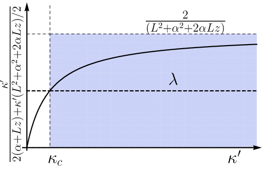
The threshold trapping rate can be written as

\kappa_{c}=\frac{2(\alpha+Lz)\lambda}{1-(L^{2}+\alpha^{2}+2\alpha Lz)\lambda/2}

(23)

This is an important result of this work. Note that when $L\rightarrow\infty$ , $\kappa_{c}\ \rightarrow\ 0.$

4.2 Trapping with logistic growth

We shall compute the population $N(t)$ for a logistic growth $F(u)=\lambda u(1-u/\bar{u})$ where $\bar{u}$ is the carrying capacity. However, unlike the linear growth case here we cannot compute population exactly due to the nonlinearity. We obtain a perturbative solution for finite time and at steady state.

4.2.1 Perturbative solution at finite time:

Inserting the expression for $F(u)$ in Eq. (1) we have

\partial_{t}u=D\partial_{x}^{2}u-\partial_{x}(\phi u)-\kappa\delta(x)u+\lambda(1-u/\bar{u})u.

(24)

Now dividing Eq. (24) through by $\bar{u}$ and using the transformation $t\rightarrow Dt$ , $\kappa\rightarrow\kappa/D$ , $\lambda\rightarrow\lambda/D$ and $u\rightarrow u/\bar{u}$ we can write

\partial_{t}u=\partial_{x}^{2}u-\partial_{x}(\phi u)-\kappa\delta(x)u+\lambda(1-u)u,

(25)

with the boundary condition $\lim_{|x|\rightarrow\infty}u=0$ and initial condition $u(x,0)=\delta(x-a)/\bar{u}$ . Let $u=u_{0}+\lambda u_{1}+\ldots$ so that we have

	$\displaystyle\mathcal{O}(1):~~~$	$\displaystyle\partial_{t}u_{0}=\partial_{x}^{2}u_{0}-\partial_{x}(\phi u_{0})-\kappa\delta(x)u_{0}$		(26)
	$\displaystyle\mathcal{O}(\lambda):~~~$	$\displaystyle\partial_{t}u_{1}=\partial_{x}^{2}u_{1}-\partial_{x}(\phi u_{1})-\kappa\delta(x)u_{1}+(1-u_{0})u_{0},$		(27)

with initial conditions $u_{0}(x,0)=\delta(x-a)/\bar{u}$ and $u_{1}(x,0)=0$ . Note that u₁ has the dimension of (length)². Taking the Laplace Transform and by using the Green’s function one can write the solution $\tilde{u}_{0}$ , the Laplace Transform of u₀ as (see Eq. (4))

\tilde{u}_{0}=\frac{1}{\bar{u}}\left(G(x|a)-\frac{\kappa G(x|0)G(a|0)}{1+\kappa G(0|0)}\right).

(28)

Note that $\tilde{u}_{0}$ has the dimension of (length)² as required. Similarly, we can write

\tilde{u}_{1}=\frac{-\kappa\tilde{R}(0,s)G(0|x)}{1+\kappa G(0|0)}+\tilde{R}(x,s),

(29)

where $\tilde{R}(x,s)=\int\tilde{r}(x^{\prime},s)G(x^{\prime}|x)dx^{\prime}$ and $\tilde{r}(x,s)$ is the Laplace transform of $u_{0}(1-u_{0})$ . We note again that $\tilde{u}_{1}$ has the requisite dimension of (length)₂. Taking the Inverse Laplace Transform of Eq. (28) gives the solution for single particle trapping case (see Eq. (4)). The contribution due to the growth term up to $\mathcal{O}(\lambda)$ can be computed from Eq. (29). For large $q$ we can write $\tilde{u}_{0}$ as

\tilde{u}_{0}\simeq\frac{1}{\bar{u}}\left\{\begin{array}[]{ll}\frac{\mbox{e}^{-q|x-a|}}{q(1+z)}-\frac{\kappa~\exp(-q(|x|+a))}{2qz(1+z)(q+\kappa/2z)}\mbox{~~if~~}|x|<\alpha\\ \frac{\mbox{e}^{-q|x-a|}}{2q}-\frac{\kappa~\exp(-q(|x|+a))}{2q(1+z)(q+\kappa/2z)}\mbox{~~if~~}\alpha<|x|<\beta.\end{array}\right.

(30)

This is an approximate solution obtained by using Eq. (13) for the Green’s function. Similarly the integrand $\tilde{r}(x,s)$ for large $q$ can be written as

\tilde{r}(x,s)\simeq\tilde{u}_{0}-\frac{2}{\pi\bar{u}^{2}}K_{0}(\sqrt{2}|x-a|q)\left\{\begin{array}[]{ll}\frac{1}{(1+z)^{2}},\mbox{~~if~~}|x|<\alpha,\\ \frac{1}{4},\mbox{~~~~~if~~}\alpha<|x|<\beta,\end{array}\right.

(31)

where $K_{0}(\cdot)$ is the modified Bessel function of the second kind. Although further approximations can be made to compute the solution $u(x,t)\simeq u_{0}(x,t)+\lambda u_{1}(x,t)$ , the expression will be too complicated and will not be very useful. Therefore, instead of examining the behavior of $u$ , we investigate that of the total population $N(t)=\bar{u}\int udx$ . The following integration gives the approximate total population

$\displaystyle\tilde{N}(s)$	$\displaystyle=\bar{u}\int_{-\beta}^{\beta}u_{0}dx+\lambda\bar{u}\int_{-\beta}^{\beta}u_{1}dx+\mathcal{O}(\lambda\kappa),$
	$\displaystyle\simeq\tilde{S}(s)+\lambda\bar{u}\int_{-\beta}^{\beta}\tilde{R}(x,s)dx,$
	$\displaystyle\simeq\tilde{S}(s)\left(1+\frac{\lambda}{q^{2}}\right)-\frac{\lambda}{2\pi\bar{u}}\int_{-\beta}^{\beta}\int^{\beta}_{\alpha}K_{0}(\sqrt{2}\|x^{\prime}-a\|q)G(x^{\prime}\|x)dx^{\prime}dx.$	(32)

where $\tilde{S}(s)$ is defined by Eq. (14). In Eq. (32) only the dominant terms are retained as other terms are exponentially small. Integrating the Green’s function we have $\int G(x^{\prime}|x)dx\sim q^{-2}$ . The integrand $K_{0}(\sqrt{2}|x^{\prime}-a|q)\sim-(\gamma+\log(q|x^{\prime}-a|/\sqrt{2}))$ if $a-c/q<x<a+c/q$ for all $q$ where $\gamma=0.577216\ldots$ is the Euler constant and $c=\sqrt{2}\exp(-\gamma)$ . For $|x^{\prime}-a|>c/q$ the approximation for $\tilde{r}_{1}(x^{\prime},t)$ is negative. The integral becomes

\int_{-\beta}^{\beta}\int^{\beta}_{\alpha}K_{0}(\sqrt{2}|x^{\prime}-a|q)G(x^{\prime}|x)dx^{\prime}dx=\int_{-\beta}^{\beta}\int^{a-c/q}_{a+c/q}K_{0}(\sqrt{2}|x^{\prime}-a|q)G(x^{\prime}|x)dx^{\prime}dx\simeq\frac{2c}{q^{3}}.

(33)

We note from Eq. (32) that the first term corresponds approximately to that of the linear growth as in Eq. (21) and (22) and from Eq. (33) the contribution $\lambda c/(\pi\bar{u}q^{3})$ reduces the population by an amount $\sim 2\lambda c\sqrt{t}/(\pi^{3/2}\bar{u})$ .

4.2.2 Steady state solution at low trapping and growth rates:

The solution to the steady state equation

\partial_{x}^{2}u-\partial_{x}(\phi u)-\kappa\delta(x)u+\lambda u(1-u)=0,

(34)

gives the density in the asymptotic long time limit. So, its solution can be used to determine the population $N_{\infty}$ . First, we consider the case where both $\lambda,\mbox{and}\kappa\ll 1$ . Let $u_{0}$ be the solution to Eq. (34) for $\kappa=0$ , $\lambda=0$ . Using the boundary conditions $\partial_{x}u(\pm\beta)=0$ and jump condition s[23] $\partial_{x}u(x^{-})=\partial_{x}u(x^{+})$ , $\exp(V(x^{-}))u(x^{-})=\exp(V(x^{+}))u(x^{+})$ where $x=\pm\alpha$ we obtain

u_{0}(x)=\left\{\begin{array}[]{ll}1&\mbox{~~~if~~~}\alpha<|x|<\beta,\\ 1/z&\mbox{~~~if~~~}|x|<\alpha.\end{array}\right.

(35)

Now, let us write $u=u_{0}+\kappa u_{1}+\kappa^{2}u_{2}+\ldots$ which on substitution into Eq. (34) gives

\mathcal{O}(\kappa):~~\partial_{x}^{2}u_{1}-\partial_{x}(\phi u_{1})-\lambda(2u_{0}-1)u_{1}=\delta(x)u_{0}.

(36)

We note that Eq. (36) has solution of the form $a\exp(kx)+b\exp(-kx)$ with $k=\sqrt{\lambda(2u_{0}-1)}$ . Furthermore, we have $\lambda(2u_{0}-1)=\lambda$ if $\alpha<|x|<\beta$ and $\lambda(2/z-1)$ if $|x|<\alpha$ . The solution $u_{1}$ can be written as

u_{1}(x)=\frac{-1}{2\Delta(0)}\left\{\begin{array}[]{ll}\cosh(k_{1}(\beta-|x|))&\mbox{~~~if~~~}\alpha<|x|<\beta,\\ \Delta(|x|)/qz&\mbox{~~~if~~~}|x|<\alpha.\end{array}\right.

(37)

where $\Delta(x)=k_{2}\cosh(k_{2}(\alpha-|x|))\cosh(k_{1}L)+k_{1}z\sinh(k_{2}(\alpha-|x|))\sinh(k_{1}L)$ , $k_{1}=\sqrt{\lambda}$ and $k_{2}=k_{1}\sqrt{2/z-1}$ . A comparison of the approximate steady state solution $u_{ss}\simeq u_{0}+\kappa u_{1}$ with the numerical solution is shown in Fig. 5.

Integration of the steady state solution gives the asymptotic population

N_{\infty}=2\bar{u}(L+\alpha/z)-\frac{\kappa\bar{u}}{\Delta(0)}\left(\sinh(k_{1}L)\left(\frac{1}{k_{1}}-\frac{1}{k_{2}}\right)+\frac{\sinh(k_{1}\alpha)\cosh(k_{1}L)}{zk_{1}}+\frac{\cosh(k_{1}\alpha)\sinh(k_{1}L)}{k_{2}}\right).

(38)

Using the smallness of the parameters Eq. (38) becomes

N_{\infty}\simeq\bar{u}\left(L+\alpha\text{e}^{-V_{0}}\right)\left(2-\frac{\kappa}{\sqrt{\lambda}}\right).

(39)

We note that depletion due to localized predation is proportional to the ratio $\kappa/\sqrt{\lambda}$ .

5 Numerical results

We consider a quartic double well potential described by $V(x)=V_{0}(1-x^{2}/a^{2})^{2}$ . The potential is symmetric and has a maximum at the origin and minima at $x=\pm a$ . The central barrier is of height $V_{0}$ . We choose this smooth double well potential to numerically investigate the model for arbitrary values of parameter $\lambda$ and $\kappa$ . The choice of this smooth $\phi^{4}$ potential also stems from our interest to examine the agreement of results, at least qualitatively, obtained from this potential with results, obtained from the square well bistable potential. Furthermore, this $\phi^{4}$ potential is widely used standard for any bistable system.

We consider a particle initially located in the right well at $x=a$ . In Fig. 6 we have plotted the evolution of the density $u(x,t)$ at time $t=0,1,10$ and $100$ for various values of trapping rate $\kappa$ . We observe that at large $t$ the density approaches a steady state density, as we have seen our bistable square well system. The steady state density is nonzero for small trapping rate and approaches zero as we increase the trapping rate. Again it is in agreement with our analytical results for our bistable square well system. We can see this in Fig. 7 where total population $N(t)$ at large time tends to zero for large values of trapping rate and approaches a finite value for sufficiently small values. This behavior can be explained by the equation,

dN/dt=-\kappa_{\text{eff}}N+\lambda^{\prime}N(1-N),

(40)

where $\lambda^{\prime}=\lambda/\bar{u}$ is the growth rate. This can be obtained from Eq. (34) if we assume that the effects of diffusion and trapping on the total population can be clubbed together by replacing the total effect by an effective decay rate $\kappa_{\text{eff}}$ . The solution $N(t)=(1-\kappa_{\text{eff}}/\lambda^{\prime})[1-\kappa_{\text{eff}}\exp(\kappa_{\text{eff}}t-\lambda^{\prime}t)/\lambda^{\prime}]^{-1}$ has the same behavior as Fig. 7. The effective decay rate can be written in terms of the asymptotic population $N_{\infty}$ as $\kappa_{\text{eff}}=\lambda^{\prime}(1-N_{\infty})$ .

The asymptotic population for various values of $\lambda$ and $\kappa$ is shown in Fig. 8. By least square fitting we found that $N_{\infty}(\kappa)=p/(q+\mbox{e}^{r\kappa})$ where $p,q$ and $r$ are constants. The parameter $r$ is positive for small values of $\lambda$ where $N_{\infty}\rightarrow 0$ for large $\kappa$ . However, as $\lambda$ increases, $r$ changes continuously from positive to negative values. So, when $\kappa\gg 1/|r|$ , $N_{\infty}\ \rightarrow p/q$ . Note that then $\kappa_{\text{eff}}$ can go from a positive to a negative value. This, in turn , leads to a nonzero steady state population. Similar threshold behavior were predicted analytically for the square double well potential case.

6 Conclusion

In this paper we studied the trapping reaction problem in a symmetric double well potential. A trap located at the middle of the central barrier of the double well potential is considered. This is done in the context of ecology where the confining potential is modelled as the habitat and the trap as localized predation. We observed that due to the confinement the asymptotic survival probability decay exponentially which in the absence of the potential shows a power law behavior. Furthermore, trapping reaction of a linearly growing population was studied where it is shown that even for an arbitrily large predation (trapping) the population does not vanish at long time. However, in presence of a confining potential, for a given range of growth rate there exist a threshold trapping rate $\kappa_{c}$ above which the population becomes extinct in the asymptotic time limit. For a logistic growth term we computed a first order perturbative solution for the total population. We also found from the steady state solution that asymptotic population depletes by a fraction $\kappa/\sqrt{\lambda}$ . Numerical studies are done for the case of a quartic potential an the results are discussed.

There can be many variations of this model. First of all, instead of a box potential, one can consider a finite height potential. Potential can have various interesting shapes. Furthermore, it is possible to have more than one routes to connect the habitats. In this case, the time evolution of survival probability can show interesting behavior. We consider all these problems in our subsequent analysis.

Appendix A Derivation of Green’s function

The Green’s function $G(x|y)$ is defined by

(s-\partial_{x}^{2}+\partial_{x}\phi)G(x|y)=\delta(x-y),

(41)

with boundary condition $G(x|y)=0$ as $x\rightarrow\infty$ . In abstract notation we can write it as $G=[s-\partial_{x}^{2}+\partial_{x}\phi]^{-1}$ . For the double square well potential $\phi=0$ except at points $x=\pm\alpha$ and $\pm\beta$ . Therefore the Greens function take the form

G=A\mbox{e}^{qx}+B\mbox{e}^{-qx},

(42)

where $A$ and $B$ are constant that depends on $y$ and $q=\sqrt{s}$ . At the point $\tilde{x}=\alpha$ the Green’s function satisfy the jump conditions $G(\tilde{x}^{+})=\exp(V_{0})G(\tilde{x}^{-})$ , $\partial_{x}G(\tilde{x}^{+})=\partial_{x}G(\tilde{x}^{-})$ and at point $\tilde{x}=\beta$ we have $\partial_{x}G(\tilde{x}|y)=0$ [23]. Similarly, jump conditions for the points $x=-\alpha$ and $-\beta$ are imposed. These jump conditions along with the continuity conditions at point $x=y$ gives

G(x|y)=\frac{1}{q\Delta}\left\{\begin{array}[]{ll}g(x|y)&\mbox{~~~if~~~}x<y\\ g(y|x)&\mbox{~~~if~~~}x>y,\end{array}\right.

(43)

where

\displaystyle g(x|y)=\left\{\begin{array}[]{ll}\cosh(q(\beta+x))F_{0}(y),&\mbox{~if~}-\beta<x<y<-\alpha,\\ \cosh(q(\beta+x))F_{3}(y),&\mbox{~if~}-\beta<x<-\alpha<y<\alpha,\\ F_{3}(y)F_{3}(-x),&\mbox{~if~}-\alpha<x<y<\alpha,\\ \cosh(q(\beta-y))F_{3}(-x),&\mbox{~if~}-\alpha<x<\alpha<y<\beta,\\ \cosh(q(\beta-y))F_{0}(x),&\mbox{~if~~~}\alpha<x<y<\beta,\\ \cosh(q(\beta-y))\cosh(q(x+\beta))z,&\mbox{~if~}-\beta<x<-\alpha<\alpha<y<\beta,\end{array}\right.

with $\Delta=\sinh(2q\alpha)(\cosh^{2}(qL)+\sinh^{2}(qL)z^{2})+\cosh(2q\alpha)\ sinh(2qL)z$ , $~L=\beta-\alpha$ ,

$\displaystyle F_{0}(x)$	$\displaystyle=\sinh(2q\alpha)F_{1}(x)+\cosh(2q\alpha)F_{2}(x)z,$	(50)
$\displaystyle F_{1}(x)$	$\displaystyle=\sinh(q(\|x\|-\alpha))\cosh(qL)+\cosh(q(\|x\|-\alpha))\sinh(qL)z^{2},$	(51)
$\displaystyle F_{2}(x)$	$\displaystyle=\cosh(q(2\alpha-\beta-\|x\|)),$	(52)
$\displaystyle F_{3}(x)$	$\displaystyle=\cosh(q(x+\alpha))\cosh(qL)+\sinh(q(x+\alpha))\sinh(qL)z.$	(53)

References

[1] S. Havlin and D. ben Avraham Adv. Phys. 36, 695 (1987).
[2] S. Redner and K. Kang Phys. Rev. A, 30, 3362(1984).
[3] B. Y. Balagurov and V. G. Vaks Sov. Phys. JETP 38, 968 (1974).
[4] M. D. Donsker and S. R. S. Varadhan Commun. Pure Appl. Math. 32, 721 (1979).
[5] P. Grassberger and I. Procaccia J. Chem. Phys. 77, 6281 (1982).
[6] P. K. Datta and A. M. Jayannavar Pramana-J. Phys. 38, 257(1992).
[7] H. Taitelbaum Physica A 200, 155(1993).
[8] G. H. Weiss, R. Kopelman, and S Havlin Phys. Rev. A 39, 446 (1989).
[9] H. Taitelbaum, R. Kopelman, G H Weiss, and S. Havlin Phys. Rev. A 41, 3116 (1990).
[10] P. K. Datta and A. M. Jayannavar Physica A 184, 135 (1992).
[11] T. M. Nieuwenhuizen and H. Brand J. Stat. Phys. 59, 53 (1990).
[12] T. Bagarti, A. Roy, K. Kundu and B. N. Dev, Physica A 405, 52 (2014).
[13] T. Bagarti and K. Kundu, Indian J. Phys., 88, 1157(2014).
[14] P. L. Krapivsky, J. M. Luck, K. Mallick, J. Stat. Phys. 154, 1430(2014).
[15] P. E. Parris, Phys. Rev. B, 40, 4928(1989).
[16] J. W. Edwards and P .E. Parris, Phys. Rev. E, 40, 8045(1989).
[17] A. M. Jayannavar, Solid State Comm., 77, 457(1991).
[18] A. M. Jayannavar and J. Kohler, Phys. Rev A, 41, 3391(1990).
[19] A. Valle, M. A Rodriguez and L. Pesquera, Phys. Rev. A, 43, 2070(1991).
[20] W. Ebeling, A. Engel, B. Esser and R. Feistel, J. Stat. Phys., 37, 369(1984).
[21] K. Spendier, S. Sugaya and V. M. Kenkre, Phys. Rev. E, 88, 06214(2013).
[22] G. Abramson and H. S Wio Chaos Soliton and Fract. 6, 1 (1995).
[23] M. M $\ddot{o}$ rsch, H. Risken and H. D. Vollmer, Z. Physik, 32, 245 (1979).