Data-Driven Allocation of Vaccines for Controlling Epidemic Outbreaks
Abstract
We propose a mathematical framework, based on conic geometric programming, to control a susceptible-infected-susceptible viral spreading process taking place in a directed contact network with unknown contact rates. We assume that we have access to time series data describing the evolution of the spreading process observed by a collection of sensor nodes over a finite time interval. We propose a data-driven robust convex optimization framework to find the optimal allocation of protection resources (e.g., vaccines and/or antidotes) to eradicate the viral spread at the fastest possible rate. In contrast to current network identification heuristics, in which a single network is identified to explain the observed data, we use available data to define an uncertainty set containing all networks that are coherent with empirical observations. Our characterization of this uncertainty set of networks is tractable in the context of conic geometric programming, recently proposed by Chandrasekaran and Shah [1], which allows us to efficiently find the optimal allocation of resources to control the worst-case spread that can take place in the uncertainty set of networks. We illustrate our approach in a transportation network from which we collect partial data about the dynamics of a hypothetical epidemic outbreak over a finite period of time.
I Introduction
Modeling and analysis of spreading processes in complex networks is a rich and interdisciplinary research field with a wide range of applications. Examples include disease propagation in human populations [2, 3, 4, 5, 6] or information spreading in social networks [7, 8, 9, 10]. A classical model of disease spreading is the susceptible-infected-susceptible (SIS) epidemic model [3, 2]. This model was originally proposed in the context of ‘unstructured’ populations [6]. Due to the current availability of accurate datasets describing complex patterns of network connectivity, the classical SIS model has been extended to model spreading processes in ‘networked’ populations using a variety of Markov models [7, 11, 12, 13, 4, 14, 15, 16, 5, 17].
There is a fast-growing body of literature on containing epidemic outbreaks given limited control resources. In the context of epidemiology, these resources can be pharmaceutical (e.g., vaccines and antidotes) as well as non-pharmaceutical actions (e.g., traffic control and quarantines). Since these resources are costly, it is of relevance to develop computational tools to optimize the allocation of resources throughout a population to control an outbreak. This problem has attracted the attention of the network science community, resulting in a variety of vaccination heuristics. For example, Cohen et al. [18] proposed a vaccination strategy, called acquaintance immunization policy, and proved it to be much more efficient than random vaccine allocation. Borgs et al. [19] studied theoretical limits in the control of spreads in undirected network by distributing antidotes. Chung et at. [20] proposed an immunization strategy based on PageRank centrality. Similar problems have also been studied recently in the communication and control community [21, 22, 23, 24, 25, 26, 27, 28, 29, 30, 31, 32, 33].
We base our work on [34, 35], where Preciado et al. developed a convex optimization framework to find the cost-optimal distribution of vaccines and antidotes in both directed and undirected networks. Although current vaccination strategies assume full knowledge about the network structure and spreading rates, in most practical applications, this information is only partially known. To elaborate on this point, let us consider the following setup. Assume that each node in a network represents subpopulations (e.g., city districts) connected by edges that are determined by commuting patterns between districts. In practice, one can use traffic information and geographical proximity to infer the existence of an edge connecting districts; however, it is very challenging to use this information to estimate the contact rates between subpopulations. Inspired by this practical realization, we consider a networked SIS model taking place in a contact network with unknown contact rates. To extract information about these unknown rates, we assume that we have access to time series data describing the evolution of the spreading process observed by a collection of sensor nodes over a finite time interval. Such time series data can be obtained from web services such as Google Flu Trends [36], or public health agencies such as the Center for Disease Control in the US [37].
A possible approach to recover the spreading rates is the use of network identification techniques [38, 39, 40, 41, 42, 43, 44, 45, 46, 47]. However, these techniques are designed to find only one of the many networks that are coherent with empirical observations [48]. Furthermore, as illustrated in [49, 50], these techniques can lead to unsuccessful network identification. In contrast to network identification techniques, we propose a data-driven robust convex optimization framework to find the optimal allocation of protection resources (e.g., vaccines and/or antidotes) over a set of control nodes to eradicate the viral spread at the fastest possible rate. In contrast to current network identification heuristics, in which a single network is identified to explain the observed data, we define an uncertainty set containing all networks that are consistent with the observed data. Our characterization of this uncertainty set of networks is tractable in the context of conic geometric programming, which has recently been proposed by Chandrasekaran and Shah [1]. In this context, we are able to efficiently find the optimal allocation of resources to control the worst-case spread that can take place in the uncertainty set of networks. We illustrate our approach in a transportation network from which we collect partial data about the dynamics of a hypothetical epidemic outbreak over a finite period of time. We discover that incorporating observations into the uncertainty set of networks significantly helps reduce the worst-case bound on the spreading rate. As we increase either the length of time over which observations are taken or the number of sensor nodes, the bound on the spreading rate decreases monotonically and converges after a relatively small number of observations (either in time or in the number of nodes). Furthermore, even though our allocation algorithm does not have access to the true underlying contact network, the resulting allocation performs surprisingly close to the full-knowledge optimal allocation.
The rest of the paper is organized as follows. In Section II, we provide some preliminaries and formulate the problem under consideration. In Section III, we introduce the conic geometric programming framework and provide the details about how to cast our problem into this framework. In Section IV, we illustrate our approach with numerical simulations using data from the air transportation network.
II Preliminaries & Problem Definition
We begin by introducing the notation and preliminary results needed in our derivations. In the rest of the paper, we denote by (respectively, ) the set of -dimensional vectors with nonnegative (respectively, positive) entries. For , we define as the set of integers . We denote vectors using boldface and matrices using capital letters. We denote by the vector of all zeros. Given two vectors and of equal dimension, indicates component-wise inequality.
II-A Graph-Theoretic Nomenclature
A weighted, directed graph is defined as the triad , where is a set of nodes, is a set of ordered pairs of nodes called directed edges, and the weight function associates positive real weights to the edges in . Throughout the paper, we may use and interchangeably for all . By convention, we say that is an edge from pointing towards . We define the in-neighborhood of node as . We define the weighted in-degree of node as . A directed path from to in is an ordered set of vertices such that for . A directed graph is strongly connected if, for every pair of nodes , there is a directed path from to . The adjacency matrix of a weighted, directed graph , denoted by , is an matrix with entries if edge , and otherwise. In this paper, we only consider graphs with positively weighted edges; hence, adjacency matrices are always nonnegative. Given an nonnegative matrix , we can always associate a directed graph such that is the adjacency matrix of . Finally, a nonnegative matrix is irreducible if and only if its associated graph is strongly connected.
Given an matrix , we denote by the eigenvalues of , where we order them according to their magnitudes, i.e., . We denote the corresponding eigenvectors by . We call the spectral radius (or dominant eigenvalue) of , which we also denote by .
II-B SIS Model in Directed Networks
In our work, we model the spread of a disease using an extension of the networked discrete-time SIS model proposed by Wang et al. in [17]. In contrast to Wang’s model, we consider directed networks (instead of undirected) with non-homogeneous transmission and recovery rates (instead of homogeneous) as described below. In all SIS models, each node can be in one out of two possible states: susceptible or infected. Over time, nodes switch their states according to a stochastic process parameterized by (i) a set of infection rates representing the rates at which an infection can be transmitted through the edges in the network, and (ii) a set of recovery rates representing the rates at which nodes recover from an infection. We define to be the probability of node being infected at a particular time slot . In the epidemiological problem considered herein, it is convenient to associate each node not to an individual, but a subpopulation living in a particular district11 1 Although in the original networked SIS model [17], nodes represented individuals in a social network, we find the interpretation of nodes as districts better-suited for epidemiological applications.. In this context, the variable represents the fraction of the population being infected at time . In the original model proposed by Wang et al. [17], the infection and recovery rates were assumed to be homogeneous, i.e., and , and the evolution of was described by a set of difference equations obtained from a mean-field approximation (see [17], eq. (5)–(6)). In our work, we consider the case of non-homogeneous contact and recovery rates, for which the set of difference equations can be easily derived to be [26]
| (1) |
for . This is a system of nonlinear difference equations for which one can derive sufficient conditions for global stability as follows. First, notice the following upper bound of (1)
| (2) |
where the last upper bound is a close approximation of (1) for and/or . For convenience, we define the complementary recovery rate of node as , and the vector . We also define the matrix of infection rates , where we assume for all pairs such that . Notice that maintains the same sparsity pattern as . Using the upper bound in (2), we define the following linear discrete-time system , , which can be written in matrix-vector form as , where and the state matrix is given by . Hence, the linear system is asymptotically stable if
| (3) |
where the spectral radius of the state matrix determines the exponential decay rate of the infection probabilities, i.e., for some . Since (2) upper bounds (1), we have that for all when . Therefore, the spectral condition in (3) is sufficient for global asymptotic stability of the nonlinear model in (1). Furthermore, the smaller the magnitude of , the faster the disease dies out.
II-C Problem Formulation
Our main objective is to find the optimal allocation of control resources to eradicate a disease at the fastest rate possible. In order to formulate our problem, we first need to describe what pieces of information are available and what control actions we are considering. In what follows, we first describe the information available. In most real epidemiological problems, researchers do not have access to the spreading rates associated to the links connecting different districts. Therefore, the exact state matrix is usually unknown. In order to extract information about the state matrix, we consider two different sources of information that are generally available in epidemiological problems. We classify these sources as (i) prior information about the network topology and parameters of the disease, and (ii) empirical observations about the spreading dynamics. In particular, we consider the following pieces of prior information:
- P1.
We assume that the sparsity pattern of the contact matrix is given, although its entries are unknown. This piece of information may be inferred from geographical proximity, commuting patterns, or the presence of transportation links connecting subpopulations.
- P2.
We assume that we know the upper and lower bounds on the spreading rates associated to each edge, i.e., , for all , which may be inferred from traffic densities and subpopulation sizes.
- P3.
In practice, each district contains a large number of individuals. Therefore, we can use the average recovery rate in the absence of vaccination as an estimation of the nodal recovery rate. We denote this ‘natural’ recovery rate by , and assume it to be known.
Apart from these pieces of prior information, we also assume that we have access to partial observations about the evolution of the spread over a finite time interval. In particular, we assume that we observe the dynamics of the disease for from a collection of sensor nodes . In other words, we have access to the following data set:
| (4) |
We assume that the data are collected before any control action is taken; therefore, the evolution of follows the dynamics in (1) with (which we assume to be known).
In what follows, we define an uncertainty set that contains all contact matrices consistent with both empirical observations and prior knowledge. Based on our prior knowledge described in items P1–P3 above, we define the following uncertainty set:
We also define to be the set of contact matrices that are coherent with the empirical observations :
The set contains those contact matrices such that the transmission rates are consistent with the ‘natural’ disease dynamics in (1) with . Notice that is defined as a collection of polynomial equality constraints on the contact rates given by (1). The uncertainty set that combines information from both prior knowledge and empirical observations is defined as
Having introduced the pieces of available information, we now describe the set of control actions under consideration. In order to eradicate the disease at the fastest rate possible, we assume that we can use pharmaceutical resources to tune the recovery rates in a collection of control nodes, i.e., for . In practice, these resources might be implemented by, for example, distributing vaccines and/or antidotes throughout the subpopulations located at those control districts. We assume that distributing vaccines in a district has an associated cost, which we represent as a node-dependent vaccine cost function. It is convenient to describe the vaccine cost function of a district in terms of its complementary recovery rate . We denote the vaccine cost function of node by . This function represents the cost of tuning the complementary recovery rate of the subpopulation at node towards the value . We assume that we can control the complementary recovery rate within a given feasible interval , where . We assume that the cost of achieving is zero, since it is equivalent to maintaining the natural recovery rate. We also assume that the maximum of in is achieved at . Furthermore, we also assume that is monotonically decreasing in the range . In other words, as we increase the level of investment to protect a given subpopulation, we also increase the recovery rate of that subpopulation.
We are now in a position to state the control problem under consideration:
Problem 1.
(Data-driven optimal allocation) Assume we are given the following pieces of information about a viral spread:
(i) prior information about the state matrix (as described in P1–P3);
(ii) a finite (and possibly sparse) data series representing partial evolution of the spread over a set of sensor nodes during the time interval (i.e., in (4));
(iii) a set of vaccine cost functions for all , and a range of feasible recovery rates such that ;
(iv) a fixed budget to be allocated throughout a set of control nodes in , so that .
Find the cost-constrained allocation of control resources to eradicate the disease at the fastest possible exponential rate, measured as , over the uncertainty set of contact matrices coherent with prior knowledge and the observations in .
From the perspective of optimization, Problem 1 is equivalent to finding the optimal allocation of resources to minimize the worst-case (i.e., maximum possible) decay rate for all . This can be cast as a robust optimization problem in the following:
| (5) | ||||||
where the first constraint accounts for our budget limit . In general, the set is nonconvex due to the observation-based uncertainty set . In Section III-C, we will define a convex superset , such that problem (5) can be relaxed into a conic geometric program. In our numerical simulations, we verify that this relaxation provides a good approximation based on real network data. From here on, we will refer to problem (5) as the robust allocation problem.
III Data-Driven Resource Allocation
In this section, we develop a mathematical framework to solve the robust allocation problem described above. Our solution is based on geometric programming [51] and its conic extension recently proposed by Chandrasekaran and Shah in [1]. We start our exposition by briefly reviewing some concepts used in our formulation.
III-A Robust Geometric Programming
Geometric programs (GPs) are a type of quasiconvex optimization problem that can be easily transformed into a convex program and solved in polynomial time. Let denote decision variables and define . In the context of GP, a monomial is defined as a real-valued function of the form with and . A posynomial function is defined as a sum of monomials, i.e., , where and . It is convenient to write down a posynomial as the product of a vector of nonnegative coefficients and a vector of monomials , such that . Notice that is the set of all monomials involved in our posynomial. Posynomials are closed under addition, multiplication, and nonnegative scaling. A posynomial can be divided by a monomial, with the result a posynomial.
A GP is an optimization problem of the form (see [51] for a comprehensive treatment):
| (6) | ||||||
where are posynomial functions and are monomials. To write in vector-product form, we can define a vector of positive coefficients such that , so that the posynomial constraints in (6) can be written as .
A GP is a quasiconvex optimization problem [52] that can be convexified using the logarithmic change of variables (see [51] for more details on this transformation). After this transformation, the GP in (6) takes the form
| (7) | ||||||
where for and (i.e., the exponents of the monomial ) for . As a result of this transformation, the optimization problem (7) is convex and can be efficiently solved in polynomial time (see [52, Chapter 4.5] for more details).
In this paper, we shall use conic GP, which is a conic extension of GP, to solve the following robust GP with coefficient uncertainties:
| (8) | ||||||
| (9) | ||||||
where is a vector of coefficients contained in an uncertainty set . The robust GP in (8) extends the formulation of the standard GP in (6) to account for uncertainties in the coefficients of the posynomial functions for .
However, the constraints (9) cannot be handled naturally by numerical optimization solvers. In what follows, we propose a methodology to rewrite these constraints in a more numerically favorable manner when the uncertainty sets in (9) can be expressed in terms of an -dimensional convex cone as follows:
| (10) |
for some fixed and . Based on the representation (10) of , we can use duality theory to derive a more numerically favorable representation of the constraint in (9) as follows. Assuming can be represented as (10), we have that for each , constraint (9) is equivalent to the optimal value of the following optimization problem satisfying :
The dual problem of the above is given by
where is the dual cone of [52]. Assume that strong duality holds in this case. Then the optimal value of the dual problem is also given by . Namely, there exists a dual feasible such that . Therefore, the constraint in (9) is equivalent to:
| (11) |
for each . For the uncertainty set used in our robust allocation problem, both and are the nonnegative orthant. Therefore, we can use the new constraints in (11) to replace those in (9) and rewrite the robust GP in (8) as
| (12) | ||||||
By applying the logarithmic transformation to (12) for all , we obtain
| (13) | ||||||
where and ( is component-wise exponential). It can be shown that both and the entries of are convex in , since they are nonnegative sums of exponentials of affine functions in [52]. In fact, problem (13) is a convex problem and is a particular instance of a conic geometric program [1]. Problems in the form of (13) can be solved efficiently using off-the-shelf software such as CVX [53].
III-B Robust Optimal Resource Allocation
In the following, we show how to formulate the optimization problem (5) as a conic GP using the methodology proposed in Section III-A. In our derivations, we use the theory of nonnegative matrices and the Perron-Frobenius lemma [54]:
Lemma 2 (Perron-Frobenius).
Suppose is an irreducible nonnegative matrix. Then, the spectral radius of satisfies:
(a) is a simple eigenvalue of ;
(b) for some ;
(c) .
Remark 3.
Note that the state matrix of the linear system (2) is irreducible if the graph is strongly connected. In what follows, we shall assume that the contact network is strongly connected. This assumption is reasonable in the context of epidemic control, since the transportation network connecting different districts or subpopulations is strongly connected in most cases. Notice also that, as a consequence of this assumption, all the matrices in the uncertainty set are irreducible.
Using item (c) in the Perron-Frobenius lemma, the spectral radius can be written as follows:
| (14) |
where in the last equality we use the fact that for any . Using (14), we rewrite the optimization problem (5) as
| (15) | ||||||
In what follows, we will first cast problem (15) into a robust GP with coefficient uncertainties. The main technical challenge we face is the --- structure in the objective function of problem (15). As we prove in Appendix -B, we can use the Saddle Point Theorem (Proposition 11, Appendix -A) to exchange the order of and , so that problem (15) can be written as
which is equivalent to:
If we introduce a slack variable
we obtain the optimization problem described in the following proposition.
Proposition 4.
Proof:
See Appendix -B. ∎Notice that the decision variables , , and of problem (16) are all strictly positive. If is a monomial for all , then problem (16) is a robust GP with coefficient uncertainties (in ). In the next, we will show that the uncertainty set can be relaxed into a convex set in the form of (10), so that problem (16) can be solved efficiently as a conic GP using the methodology proposed in Section III-A.
III-C Convex Set of Data-Coherent Networks
As we mentioned in Section II-C, the uncertainty set is nonconvex since it is defined by a collection of polynomial equalities. In this subsection, we define a convex superset , so that problem (5) becomes a conic geometric program after we substitute by (which changes the combined uncertainty set ).
We define the convex superset as follows:
| (18) |
Lemma 5.
The set is a superset of .
Proof:
Consider any . Recall that it always holds that . Then, from the AM-GM inequality, we have that
| (19) |
We can use (19) to yield a constraint on the transmission rates from the empirical dataset defined in (4). Applying (19) to the nonlinear dynamics (1) results in the following inequality:
where we have used the fact that the recovery rate is equal to the natural recovery rate during empirical observations. Since , we can rearrange the above inequality to obtain
which is equivalent to
| (20) |
Here we have used the fact
according to the system dynamics (1). We can rearrange (20) to obtain
Finally, we use the fact
to complete the proof. ∎The following comments are in order. First, the uncertainty set in (18) is defined by a collection of affine inequalities; therefore, it is a convex polytope and can be represented in the form of (10). Second, from Lemma 5, we have that the superset contains all the contact matrices that are coherent with both prior information and empirical observations. In the following section, we illustrate our relaxation with numerical simulations and verify that the robust allocation is not overly conservative. In fact, for some realistic cases, the robust allocation achieves similar performance as the optimal allocation solved under a known contact matrix .
IV Simulations
In this section, we illustrate the robust data-driven allocation framework developed in Section III. We consider the problem of controlling an epidemic outbreak propagating through the worldwide air transportation network [55]. The nodes in the network represent airports, whereas edges are flight connections for which we know passenger flows. Through our simulations, we demonstrate the following facts about the data-driven allocation framework. First, incorporating observations into the uncertainty set significantly helps reduce the worst-case spreading rate bound. Second, the robust allocation framework does not need many observations to converge; in particular, the length of the observation period that we need is only a fraction of the number of nodes in the network. Finally, even though the robust allocation algorithm does not have access to the true underlying contact network , the resulting allocation achieves very similar performance compared to the optimal allocation solved using the actual .
IV-A Numerical Setup

In our simulations, we consider the problem of controlling an epidemic outbreak propagating through a flight network comprised by the top airports (based on yearly total traffic), so that . To illustrate the robust data-driven approach, we first generate a time series representing the dynamics of a hypothetical outbreak using the nonlinear dynamics (1). We run our simulation assuming a homogeneous value for the natural recovery rate, for all , and a link-dependent contact rate that is proportional to the traffic through that edge. Assuming an initial infection for all , we generate a time series representing the evolution of the infection over time.
In our data-driven framework, we assume that we do not have direct access to the matrix of infection rates . Instead, the data-driven allocation algorithm only has access to the observations for some period . Using this data, our algorithm generates an uncertainty set of data-coherent contact matrices. The parameters that define the uncertainty set are chosen as follows. For all , we assume an a priori upper bound (i.e., the contact rate of an edge is at most 50% above its nominal contact rate), whereas the lower bound is (i.e., the contact rate is at least half the nominal value). The natural recovery rate is chosen as for all , while the lower bound is chose to be for all (i.e., the recovery rate is at most ). We assume that the set of control nodes and vary the set of sensing nodes.
To find the optimal allocation of vaccines, we consider the following vaccination cost function given by
for all . It can be seen that is a monomial in . The function satisfies ; namely, there is no cost by keeping as the natural complementary recovery rate . This function also satisfies ; namely, the maximum allocation per node is one unit. Furthermore, the cost function is monotonically decreasing and exhibits diminishing returns (see Fig. 1). In this setup, our problem is to find the optimal allocation of vaccines throughout the airports in the air transportation network assuming we have a total budget equal to .
IV-B Results and Discussions
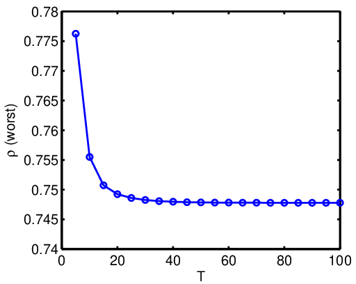
For any given uncertainty set , we define the worst-case spectral radius as the optimal value of the robust allocation problem (5). In other words, represents the slowest exponential rate of disease eradication that can be achieved for those contact matrices that are coherent with our observations. In our first experiment, we illustrate the dependency of with respect to , i.e., the number of observations available. In Fig. 2, we show the value of as we increase the observation period in the range . Notice how, as grows, the amount of available information about the contact network increases and, as a result, decreases (i.e., we are able to guarantee a faster disease eradication). Notice also that the value of remains approximately unchanged after observations. This result may seem surprising at first glance, since from the perspective of system observability, one would normally need as many time steps as the dimension of the system (in this case, ) in order to identify the system. This demonstrates one of the benefits of using the robust allocation framework; namely, it allows us to find an allocation without performing a previous system identification.
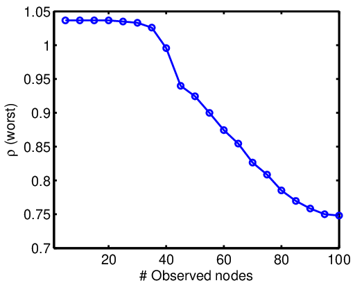
In a second set of experiments, we numerically verify the performance of our data-driven allocation algorithm in the presence of sparse observations. In particular, we assume that we can only measure the evolution of the disease in a set of sensor nodes , which we choose to be those airports with the highest yearly total traffic. In Fig. 3, we plot the value of as we increase the number of sensor nodes from . Notice how, as we increase the number of sensor nodes, decreases. Interestingly, for sensors, the value of hardly changes. In contrast, we observe a dramatic improvement in the value of for . In fact, using only 40 sensors (out of 100 nodes), we can find an allocation that guarantees the eradication of the disease (i.e., ), even for the worst instantiation of in .
In our final simulation, we compare the allocation obtained from the data-driven framework with the allocation obtained assuming we have full access to the actual matrix of infection rates . Using the framework proposed in Preciado et al. [35], we can obtain the optimal allocation , which is defined as the solution to the following optimization problem:
| (21) | ||||||
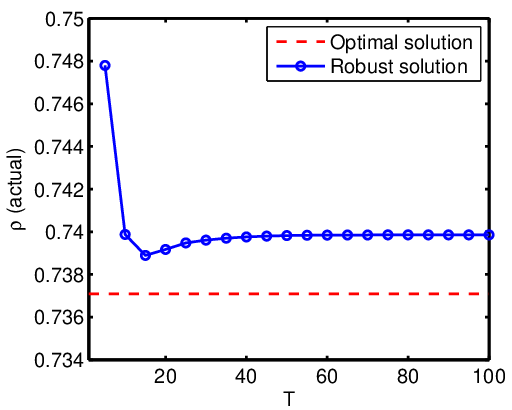
The optimal value of problem (21) represents the fastest exponential rate at which the disease is eradicated when the contact network is completely known. Additionally, we denote by the optimal solution to the robust data-driven allocation problem (5) when time samples are available. We evaluate the spectral radius , which represents the exponential rate at which the disease is eradicated when we apply the allocation to the actual contact network . In Fig. 4, we compare with the optimal value for different values of . Since is the optimal solution to problem (21), we always have . However, Fig. 4 shows that the difference between and is small for the particular network under investigation.
Finally, it is worth mentioning that the robust data-driven allocation problem does not take significantly more time to solve than the optimal allocation problem. We have solved both allocation problems in MATLAB (R2012b) using CVX (Version 2.1, Build 1079) [53] with the Mosek solver (Version 7.0.0.106). All computations are carried out on a laptop computer equipped with a dual-core 2.5 GHz Intel Core i5 processor and 4 GB of RAM. For , the optimal allocation problem takes approximately 17 seconds to solve, whereas the robust allocation problem with a priori bounds on takes approximately 49 seconds for .
V Conclusions
We have introduced a novel mathematical framework, based on conic geometric programming, to control a viral spreading process taking place in a contact network with unknown contact rates. We assume that we have access to time series data describing the evolution of the spreading process over a finite time period over a collection of sensor nodes. Using this data, we have developed a data-driven robust convex optimization framework to find the optimal allocation of protection resources over a set of control nodes to eradicate the viral spread at the fastest possible rate.
We have illustrated our approach using data obtained from the worldwide air transportation network. We have simulated a hypothetical epidemic outbreak over a finite time period and fed the resulting time series in our data-driven optimization algorithm. From our numerical results, we verify that (i) incorporating observations into the data-driven allocation algorithm significantly reduces the worst-case spreading rate bound; (ii) the robust allocation framework does not need many observations to converge; (iii) even though the robust allocation algorithm does not have access to the true underlying contact network , the resulting allocation achieves very similar performance compared to the optimal allocation solved under the actual .
References
- [1] V. Chandrasekaran and P. Shah, “Conic geometric programming,” in Annual Conference on Information Sciences and Systems, pp. 1–4, 2014.
- [2] N. Bailey, The Mathematical Theory of Infectious Diseases and Its Applications. Charles Griffin & Company Ltd., 1975.
- [3] R. M. Anderson, R. M. May, and B. Anderson, Infectious Diseases of Humans: Dynamics and Control, vol. 28. Wiley, 1992.
- [4] M. Newman, “Spread of epidemic disease on networks,” Physical Review E, vol. 66, no. 1, p. 016128, 2002.
- [5] R. Pastor-Satorras and A. Vespignani, “Epidemic dynamics and endemic states in complex networks,” Physical Review E, vol. 63, p. 066117, May 2001.
- [6] G. H. Weiss and M. Dishon, “On the asymptotic behavior of the stochastic and deterministic models of an epidemic,” Mathematical Biosciences, vol. 11, no. 3, pp. 261–265, 1971.
- [7] M. Draief and L. Massoulié, Epidemics and Rumours in Complex Networks. Cambridge University Press, 2010.
- [8] D. Easley and J. Kleinberg, Networks, Crowds, and Markets. Cambridge University Press, 2010.
- [9] D. Kempe, J. Kleinberg, and E. Tardos, “Maximizing the spread of influence through a social network,” in ACM SIGKDD, pp. 137–146, 2003.
- [10] J. Leskovec, L. A. Adamic, and B. A. Huberman, “The dynamics of viral marketing,” ACM Transactions on the Web, vol. 1, no. 1, p. 5, 2007.
- [11] A. J. Ganesh, L. Massoulié, and D. F. Towsley, “The effect of network topology on the spread of epidemics,” in IEEE INFOCOM 2005, vol. 2, pp. 1455–1466, 2005.
- [12] P. Van Mieghem, J. Omic, and R. Kooij, “Virus spread in networks,” IEEE/ACM Transactions on Networking, vol. 17, no. 1, pp. 1–14, 2009.
- [13] Y. Moreno, R. Pastor-Satorras, and A. Vespignani, “Epidemic outbreaks in complex heterogeneous networks,” The European Physical Journal B, vol. 26, pp. 521–529, 2002.
- [14] V. M. Preciado and A. Jadbabaie, “Spectral analysis of virus spreading in random geometric networks,” in IEEE Conference on Decision and Control, pp. 4802–4807, 2009.
- [15] V. M. Preciado and A. Jadbabaie, “Moment-based analysis of spreading processes from network structural information,” IEEE Transactions on Automatic Control, vol. 21, no. 2, pp. 373–382, 2013.
- [16] R. Pastor-Satorras and A. Vespignani, “Epidemic dynamics in finite size scale-free networks,” Physical Review E, vol. 65, no. 3, p. 035108, 2002.
- [17] Y. Wang, D. Chakrabarti, C. Wang, and C. Faloutsos, “Epidemic spreading in real networks: An eigenvalue viewpoint,” in IEEE Symposium on Reliable Distributed Systems, pp. 25–34, 2003.
- [18] R. Cohen, S. Havlin, and D. Ben-Avraham, “Efficient immunization strategies for computer networks and populations,” Physical Review Letters, vol. 91, no. 24, p. 247901, 2003.
- [19] C. Borgs, J. Chayes, A. Ganesh, and A. Saberi, “How to distribute antidote to control epidemics,” Random Structures & Algorithms, vol. 37, no. 2, pp. 204–222, 2010.
- [20] F. Chung, P. Horn, and A. Tsiatas, “Distributing antidote using pagerank vectors,” Internet Mathematics, vol. 6, no. 2, pp. 237–254, 2009.
- [21] Y. Wan, S. Roy, and A. Saberi, “Designing spatially heterogeneous strategies for control of virus spread,” IET Systems Biology, vol. 2, no. 4, pp. 184–201, 2008.
- [22] P. Van Mieghem, J. Omic, and R. Kooij, “Virus spread in networks,” IEEE/ACM Transactions on Networking, vol. 17, no. 1, pp. 1–14, 2009.
- [23] F. Sahneh and C. Scoglio, “Epidemic spread in human networks,” in IEEE Conference on Decision and Control, pp. 3008–3013, 2011.
- [24] F. D. Sahneh, C. Scoglio, and P. Van Mieghem, “Generalized epidemic mean-field model for spreading processes over multilayer complex networks,” IEEE/ACM Transactions on Networking, vol. 21, pp. 1609–1620, Oct. 2013.
- [25] P. Van Mieghem and J. Omic, “In-homogeneous virus spread in networks,” arXiv preprint arXiv:1306.2588, 2013.
- [26] H. J. Ahn and B. Hassibi, “Global dynamics of epidemic spread over complex networks,” in IEEE Conference on Decision and Control, pp. 4579–4585, 2013.
- [27] A. Khanafer, T. Basar, and B. Gharesifard, “Stability properties of infected networks with low curing rates,” in American Control Conference, pp. 3579–3584, 2014.
- [28] K. Drakopoulos, A. Ozdaglar, and J. N. Tsitsiklis, “An efficient curing policy for epidemics on graphs,” arXiv preprint arXiv:1407.2241, 2014.
- [29] X. Chen and V. M. Preciado, “Optimal coinfection control of competitive epidemics in multi-layer networks,” in IEEE Conference on Decision and Control, 2014.
- [30] W. Mei and F. Bullo, “Modeling and analysis of competitive propagation with social conversion,” in IEEE Conference on Decision and Control, 2014.
- [31] E. Ramirez-Llanos and S. Martinez, “A distributed algorithm for virus spread minimization,” in American Control Conference, pp. 184–189, 2014.
- [32] C. Nowzari, V. M. Preciado, and G. J. Pappas, “Stability analysis of generalized epidemic models over directed networks,” in IEEE Conference on Decision and Control, 2014.
- [33] Y. Hayel, S. Trajanovski, E. Altman, H. Wang, and P. Van Mieghem, “Complete game-theoretic characterization of SIS epidemics protection strategies,” in IEEE Conference on Decision and Control, 2014.
- [34] V. M. Preciado, M. Zargham, C. Enyioha, A. Jadbabaie, and G. J. Pappas, “Optimal vaccine allocation to control epidemic outbreaks in arbitrary networks,” in IEEE Conference on Decision and Control, pp. 7486–7491, 2013.
- [35] V. M. Preciado, M. Zargham, C. Enyioha, A. Jadbabaie, and G. J. Pappas, “Optimal resource allocation for network protection against spreading processes,” IEEE Transactions on Control of Networked Systems, vol. 1, no. 1, pp. 99–108, 2014.
- [36] “Google flu trends.” http://www.google.org/flutrends/us (retrieved: November 12, 2014).
- [37] “Flu activity & surveillance—seasonal influenza (flu).” http://www.cdc.gov/flu/weekly/fluactivitysurv.htm. (retrieved: November 12, 2014).
- [38] D. Materassi and G. Innocenti, “Topological identification in networks of dynamical systems,” IEEE Transactions on Automatic Control, vol. 55, no. 8, pp. 1860–1871, 2010.
- [39] D. Materassi and G. Innocenti, “Unveiling the connectivity structure of financial networks via high-frequency analysis,” Physica A, vol. 388, no. 18, pp. 3866–3878, 2009.
- [40] J. Gonçalves and S. Warnick, “Necessary and sufficient conditions for dynamical structure reconstruction of LTI networks,” IEEE Transactions on Automatic Control, vol. 53, no. 7, pp. 1670–1674, 2008.
- [41] Y. Yuan, G. B. Stan, S. Warnick, and J. Gonçalves, “Robust dynamical network structure reconstruction,” Automatica, 2011.
- [42] M. Timme, “Revealing network connectivity from response dynamics,” Physical Review Letters, vol. 98, no. 22, p. 224101, 2007.
- [43] M. Nabi-Abdolyousefi and M. Mesbahi, “Sieve method for consensus-type network tomography,” IET Control Theory & Applications, vol. 6, no. 12, pp. 1926–1932, 2012.
- [44] M. Nabi-Abdolyousefi and M. Mesbahi, “Network identification via node knockout,” IEEE Transactions on Automatic Control, vol. 57, no. 12, pp. 3214–3219, 2012.
- [45] S. Shahrampour and V. M. Preciado, “Reconstruction of directed networks from consensus dynamics,” in American Control Conference, pp. 1685–1690, 2013.
- [46] S. Shahrampuor and V. M. Preciado, “Topology identification of directed dynamical networks via cross-spectral analysis,” IEEE Transactions on Automatic Control, 2014.
- [47] M. Fazlyab and V. M. Preciado, “Robust topology identification and control of LTI networks,” in IEEE GlobalSIP Symposium on Network Theory, 2014.
- [48] D. Napoletani and T. D. Sauer, “Reconstructing the topology of sparsely connected dynamical networks,” Physical Review E, vol. 77, no. 2, p. 26103, 2008.
- [49] C. D. Michener and R. R. Sokal, “A quantitative approach to a problem in classification,” Evolution, pp. 130–162, 1957.
- [50] D. Marinazzo, M. Pellicoro, and S. Stramaglia, “Kernel method for nonlinear granger causality,” Physical Review Letters, vol. 100, no. 14, p. 144103, 2008.
- [51] S. Boyd, S.-J. Kim, L. Vandenberghe, and A. Hassibi, “A tutorial on geometric programming,” Optimization and Engineering, vol. 8, no. 1, pp. 67–127, 2007.
- [52] S. Boyd and L. Vandenberghe, Convex Optimization. Cambridge University Press, 2004.
- [53] CVX Research, Inc., “CVX: Matlab software for disciplined convex programming, version 2.0.” http://cvxr.com/cvx, Aug. 2012.
- [54] C. D. Meyer, Matrix Analysis and Applied Linear Algebra. SIAM, 2000.
- [55] C. M. Schneider, T. Mihaljev, S. Havlin, and H. J. Herrmann, “Suppressing epidemics with a limited amount of immunization units,” Physical Review E, vol. 84, p. 061911, Dec 2011.
- [56] D. Bertsekas, A. Nedić, and A. Ozdaglar, Convex Analysis and Optimization. Athena Scientific, 2003.
-A The Saddle Point Theorem
The purpose of this section is to present the Saddle Point Theorem from convex analysis that is used in the proof of Proposition 4. Most of this section is adopted from Chapters 1 and 2 of the book by Bertsekas et al. [56]. To prepare for this, we first introduce some basic concepts in convex analysis.
Definition 6 (Epigraph).
Let be a subset of . The epigraph of an extended real-valued function is defined as the set
Definition 7 (Closed Function).
Let be a subset of . An extend real-valued function is called closed if its epigraph is a closed set.
Definition 8 (Convex Function).
Let be a convex subset of . An extended real-valued function is called convex if is a convex set.
Let and be nonempty convex subsets of and , respectively. The Saddle Point Theorem considers a real-valued function and provides conditions to ascertain the minimax equality
| (22) |
Before introducing the Saddle Point Theorem, for each , we define the function as
and, for each , we define the function as
We also need the following assumption on and (or equivalently, ).
Assumption 9.
The function is closed and convex for each , and the function is closed and convex for each .
Remark 10.
One useful sufficient condition for the function to be closed is that the set is closed and the function is lower semicontinous in . In addition, the convexity of is equivalent to the convexity of in over . A similar sufficient condition can also be applied to .
We are now ready to present the Saddle Point Theorem.
Proposition 11 (Saddle Point Theorem).
- 1.
and are compact.
- 2.
is compact, and there exists and such that the set
is nonempty and compact.
- 3.
is compact, and there exists and such that the set
is nonempty and compact.
- 4.
There exist , , and such that the sets
are nonempty and compact.
-B Proof of Proposition 4
Without loss of generality, we assume that the vector satisfies . Define the set
We wish to show that the following minimax equality holds:
| (23) |
Define for all and the function
Then, the minimax equality (23) holds if and only if the following equality holds:
| (24) |
where .
Using the sufficient conditions in Remark 10, it can be verified that satisfies Assumption 9. To apply the Saddle Point Theorem (Proposition 11), we substitute , , , and in the Saddle Point Theorem. Since is compact according to item (i) in the formulation of Problem 1, we can apply the second condition in the Saddle Point Theorem if we can show that there exist and such that the set
| (25) |
is nonempty and compact.
Consider any and choose . We can observe that is nonempty, since . In order to show that is compact, notice that is a subset of . Then, compactness of is equivalent to that is closed and bounded as a result of the Heine–Borel theorem. To show that is closed, we use the fact that is continuous in , and is the preimage of the closed set . To show that is bounded, suppose by contradiction that is unbounded, which implies that there exists such that and for all . Substituting into (25), we obtain
for all . Define . We know that the set is nonempty; otherwise we have and hence . Then, from the irreducibility of , we know that there exist and such that . Using the definition of , we know that . As , we have and hence , which leads to a contradiction.
To summarize, we have shown that is compact and there exists such that is nonempty and compact. Then, from the second condition in the Saddle Point Theorem, we know that the minimax equality (24) holds. This allows us to rewrite the objective of problem (15) as
By introducing a slack variable
we obtain the optimization problem described in Proposition 4, where the constraint (17) is given by the definition of .