Consistent Collective Matrix Completion under Joint Low Rank Structure

Matrices are denoted by uppercase letters, $X$, $M$, etc. Matrix inner product is given by $\langle X,Y\rangle=\sum_{(i,j)}X_{ij}Y_{ij}$. The set of symmetric matrices of dimension $N$ is denoted as $\mathbb{S}^{N}$. For $M\in\mathbb{R}^{m\times n}$, with singular values $\sigma_{1}\geq\sigma_{2}\geq\ldots$, common matrix norms include the nuclear norm $\|M\|_{*}=\sum_{i}\sigma_{i}$, the spectral norm $\|M\|_{2}=\sigma_{1}$, and the Frobenius norm $\|M\|_{F}=\sqrt{\sum_{i}\sigma_{i}^{2}}=\sqrt{\sum_{ij}M_{ij}^{2}}$.

A collective–matrix, denoted using script letters, $\mathcal{X}$, $\mathcal{M}$, etc., is a collection of affinity relations among a set of $K$ types of entities; and is primarily represented as a list of $V$ matrices, $\mathcal{X}=[X_{v}]_{v=1}^{V}=[X_{v}:v=1,2,\ldots,V]$. Each component matrix $X_{v}$, called a view, is the affinity matrix between a pair of entity types denoted by ${r_{v}}$ (entity type along rows) and $c_{v}$ (entity type along columns). We only consider static undirected affinity relations, wherein, for a given pair of entity types $k_{1},k_{2}\in\{1,2,\ldots K\}$, there is at most one affinity relation $X_{v}$ defined between $k_{1}$ and $k_{2}$.

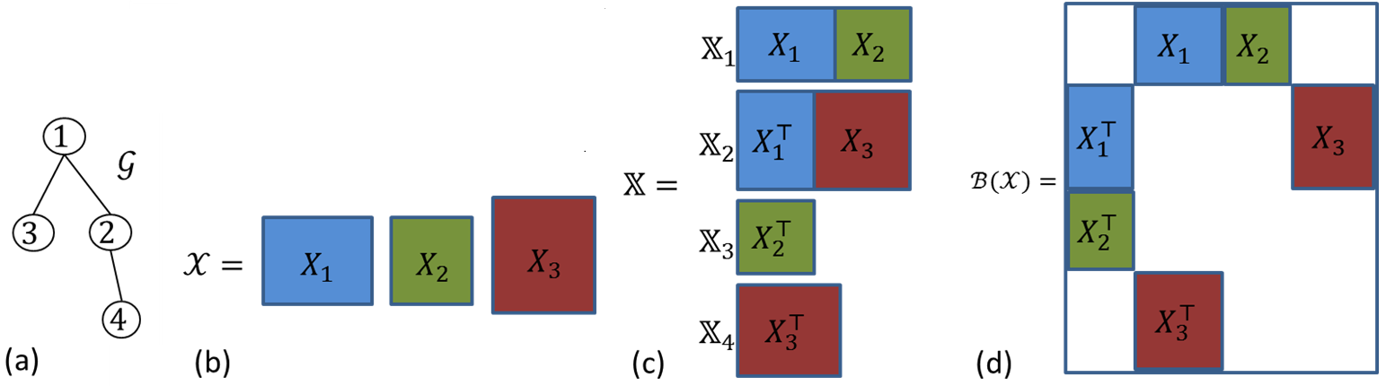
The entity–relationship structure defining a collective–matrix is represented by an undirected graph $\mathcal{G}$, with nodes denoting the $K$ entity types, and an edge between nodes $k_{1}$ and $k_{2}$ implying that a view $X_{v}$ with either $(r_{v}\,=\,k_{1},c_{v}=k_{2})$ or $(r_{v}=k_{2},c_{v}=k_{1})$ exists in the collective matrix. We assume that the graph $\mathcal{G}$ forms a single connected component, if not, each connected component could be handled separately without loss of generality. An illustration of a collective matrix structure $\mathcal{X}$ and its entity–relationship graph $\mathcal{G}$ is given in Fig. 1 $(a)$–$(b)$.

For $k=1,2,\ldots,K$, denote the number of instances of the $k^{\text{th}}$ entity type by $n_{k}$; let $N=\sum_{k}n_{k}$. Then, $\forall v$, $X_{v}\in\mathbb{R}^{n_{r_{v}}\times n_{c_{v}}}$, and collective–matrices with common entity–relationship graph $\mathcal{G}$ belong to the space:

Finally, $\forall v$, $\mathcal{I}(v)=\{(i,j):i\in[n_{r_{v}}],j\in[n_{c_{v}}]\}=[n_{r_{v}}]\times[n_{c_{v}}]$ denotes the set indices representing the elements in view $v$, where $[N]=\{1,2,\ldots,N\}$.

1. Collective–Matrix Inner Product and Euclidean Norm

   $$\langle\mathcal{X},\mathcal{Y}\rangle=\sum_{v=1}^{V}\langle X_{v},Y_{v}\rangle,\text{ and }\|\mathcal{X}\|_{F}=\sqrt{\langle\mathcal{X},\mathcal{X}\rangle}.$$

   Note: We overload the notation for inner product $\langle\cdot,\cdot\rangle$, and the Frobenius norm $\|\cdot\|_{F}$ for matrices and collective–matrices, with operands providing disambiguation.

2. Standard Orthonormal Basis

   The standard orthonormal basis for $\mathfrak{X}$ is given by $\{\mathcal{E}^{(v,i_{v},j_{v})}:v\in[V],(i_{v},j_{v})\in\mathcal{I}(v)\}$, where $\mathcal{E}^{(v,i_{v},j_{v})}\in\mathfrak{X}$ has a value of $1$ in the $(i_{v},j_{v})^{\text{th}}$ element of view $v$, and $0$ everywhere else. Recall that $[n]=\{1,2,\ldots,n\}$, and $\mathcal{I}(v)=[n_{r_{v}}]\times[n_{c_{v}}]$.

3. Joint Factorization and Collective–Matrix Rank

   A collective-matrix $\mathcal{X}\in\mathfrak{X}$ is said to possess an $R$–dimensional joint factorization, if there exists a set of factors $\{U_{k}\in\mathbb{R}^{n_{k}\times R}\}_{k=1}^{K}$, such that $\forall v,\;X_{v}=U_{r_{v}}U_{c_{v}}^{\top}$. The set of collective–matrices in $\mathfrak{X}$ that have a joint factorization structure of finite dimension is denoted by $\bar{\mathfrak{X}}\subseteq\mathfrak{X}$. For $\mathcal{X}\in\bar{\mathfrak{X}}$, the collective–matrix rank is defined as the minimum value of $R$ such that an $R$–dimensional joint factorization exists for $\mathcal{X}$.

Consider the following set of rank–$1$ collective–matrices:

where $\text{conv}()$ and $\text{ext}()$ return the convex hull and the extreme points of a set, respectively. Recall that $N=\sum_{k}n_{k}$, and $P_{v}:\mathbb{S}^{N}\to\mathbb{R}^{n_{r_{v}}\times n_{c_{v}}}$ extracts the block corresponding to the view $v$ in an $N\times N$ symmetric matrix. From the block matrix representation (Sec. 2.2.1), note that $\mathfrak{X}=\text{aff}(\mathscr{A})$; and the following proposition can be easily verified:

We define the following quantities of interest:

• Collective–Matrix Atomic Norm:

  also the gauge of $\mathscr{A}$,

  $\displaystyle\|\mathcal{X}\|_{\mathscr{A}}:=\text{inf}\{t>0:\mathcal{X}\in t\cdot\text{conv}(\mathscr{A})\}.$

  (2)

• Support function of $\mathscr{A}$:

  $\displaystyle\|\mathcal{X}\|_{\mathscr{A}}^{*}:=\text{sup}\{\langle\mathcal{X},\mathcal{A}\rangle:\mathcal{A}\in\mathscr{A}\}.$

  (3)

• “sign” collective–matrices of $\mathcal{X}$:

  $\displaystyle\mathscr{E}(\mathcal{X})=\{\mathcal{E}:\|\mathcal{X}\|_{\mathscr{A}}=\langle\mathcal{E},\mathcal{X}\rangle,\|\mathcal{E}\|_{\mathscr{A}}^{*}=1\}.$

  (4)

Remarks

1. 1.

   $\|\mathcal{X}\|_{\mathscr{A}}$ is not always a norm. It is a norm if $\mathscr{A}$ is centrally symmetric, i.e. if $\mathcal{A}\in\mathscr{A}\Leftrightarrow-\mathcal{A}\in\mathscr{A}$.

2. 2.

   By convention, $\|\mathcal{X}\|_{\mathscr{A}}=\infty$ if $\mathcal{X}\in\mathfrak{X}\setminus\bar{\mathfrak{X}}$.

3. 3.

   However, $\|\mathcal{X}\|_{\mathscr{A}}$ is always a convex function and exhibits many norm–like properties. $\forall\mathcal{X}\in\mathfrak{X}$, $\|\mathcal{X}\|_{\mathscr{A}}\geq 0$ and $\|\mathcal{X}\|_{\mathscr{A}}=0$ iff $\mathcal{X}=0$; $\forall a\geq 0,\;\|a\mathcal{X}\|_{\mathscr{A}}=a\|\mathcal{X}\|_{\mathscr{A}}$; and $\|\mathcal{X}+\mathcal{Y}\|_{\mathscr{A}}\leq\|\mathcal{X}\|_{\mathscr{A}}+\|\mathcal{Y}\|_{\mathscr{A}}$.

4. 4.

   If $\|\mathcal{X}\|_{\mathscr{A}}$ is a norm, then $\|\mathcal{X}\|_{\mathscr{A}}^{*}$ is its dual norm.

Collective–matrix completion is in general an ill–posed problem. However, recent literature on related tasks of compressed sensing [12, 7, 8], matrix estimation [28, 6, 5, 19, 20, 25, 18, 15], and other high dimensional estimation [26, 9, 4, 36] etc. propose tractable estimators with strong statistical guarantees for such high dimensional problems when low dimensional structural constraints are imposed on the ground truth parameters.

Analogous to matrices, $\forall\mathcal{X}\in\bar{\mathfrak{X}}$, we define the following:

where we have used the entity matrix set representation in (8) (See Sec. 2.2.1). In the rest of the paper, we denote $T(\mathcal{M})$ and $T^{\perp}(\mathcal{M})$ simply as $T$ and $T^{\perp}$, respectively. Let $P_{T}$ and $P_{T^{\perp}}$ be projections onto $T$ and $T^{\perp}$, respectively.

As with matrix completion, in a localized observation setting, consistent recovery is infeasible if any entry in $\mathcal{M}$ is overly significant. Such cases are precluded through the following analogue of incoherence conditions [6, 14].

Further, in Section 2.3 it was noted that in general $\bar{\mathfrak{X}}\subseteq{\mathfrak{X}}$, and the set of atoms spanning $\bar{\mathfrak{X}}$ defined in (1) need not be centrally symmetric. This poses subtle challenges in analyzing the consistency of collective–matrix completion. To mitigate these difficulties, we consider a restricted set of collective–matrix structures, under which $\mathfrak{X}=\bar{\mathfrak{X}}$, and $\mathscr{A}$ is centrally symmetric.

$\forall k$, we define $\Omega_{k}=\{(v_{s},i_{s},j_{s})\in\Omega:r_{v_{s}}=k\text{ or }c_{v_{s}}\}$. Let $|\Omega_{k}|$ be the expected number of observations in $\Omega_{k}$.

Collective–matrix rank of $\mathcal{M}\in\bar{\mathfrak{X}}$ is given by:

where $\mathcal{A}_{r}\in\mathscr{A}$. However, minimizing the rank of a collective–matrix is intractable. We use the atomic norm (2) as a convex surrogate for the rank function and propose the following convex estimator for the noise–free model:

For the additive–noise model, we suitably modify the above convex program to propose three equivalent estimators:

The estimators are theoretically equivalent in the sense that for some combination of $\omega$, $t$, and $\gamma$ we obtain the same estimate from the three convex programs. In practice, the parameters are set through cross validation, and the choice of a convex program for noisy collective–matrix completion is often made by the algorithmic considerations.

Recall: $|\Omega_{k}|$ is the expected cardinality of $\Omega_{k}=\{(v,i,j)\in\Omega:r_{v}=k\text{ or }c_{v}=k\}$, with the true cardinality concentrating sharply under the sampling scheme (Assumption 4), and $|\Omega|$ is the cardinality of $\Omega$; $n_{k}$ is the number of instances of type $k$, and $N=\sum_{k}n_{k}$; $R$ is the collective–matrix rank of $\mathcal{M}$; and $\mu_{0}$ and $\mu_{1}$ are the incoherence parameters (Assumption 2).

Recently, Jaggi et. al. [17] proposed a scalable approximate algorithm for solving nuclear norm regularized matrix estimation, by adapting the approximate SDP solver of Hazan [16]. We observe that using the alternate formulation of collective–matrix atomic norm stated in Proposition 4, the convex program for noisy collective–matrix completion in (15) can be cast as the following SDP:

where $\Omega_{v}=\{(v_{s},i_{s},j_{s})\in\Omega:v_{s}=v\}$. Hazan’s algorithm for solving (17) is given in Algorithm 1.

In comparison, the SVT–CMC algorithm proposed by Bouchard et. al. [2] converges faster in $O(\frac{1}{\sqrt{\epsilon}})$ iterations; however, each iteration in SVT–CMC requires computing all the non–zero eigen vectors of a $N\times N$ matrix, which does not scale well with $N$. Hazan’s algorithm can be used to trade–off computation for accuracy in large datasets.

A collective–matrix $\mathcal{M}$ of collective–matrix rank $R$ lies in a lower dimensional model space spanned by the entity factors, $\{U_{k}\in\mathbb{R}^{n_{k}\times R}\}$. Given $k$, $U_{k}$ is estimated entirely from $P_{\Omega_{k}}(\mathbb{M}_{k})$. Thus, an immediate lower bound on the sample complexity for well–posedness is given by $|\Omega_{k}|\sim O(n_{k}R)$. The results presented in the paper are optimal upto a poly–logarithmic factor.

A trivial estimate for collective–matrix completion is to estimate each component matrices independently. Since a joint low rank structure also imposes low rank structure on the component matrices, this is feasible if each component matrix satisfies the sample complexity requirements of standard matrix completion, i.e. $|\Omega_{v}|>C\max{\{\mu_{0},\mu_{1}\}}R(n_{r_{v}}+n_{c_{v}})\log(n_{r_{v}}+n_{c_{v}})$. Another, estimate from standard matrix completion can be obtained by completing each matrix $\{\mathbb{M}_{k}\}$ in the entity–matrix set representation independently, this requires a sample complexity of $|\Omega_{k}|>C\max{\{\mu_{0},\mu_{1}\}}R(n_{k}+m_{k})\log(n_{k}+m_{k})$ for consistent recovery. In comparison to the sample complexity in Theorem 6, these results are sub–optimal as they do not completely leverage the shared structure introduced by the jointly factorizability of collective–matrices.

Finally, the collective–matrix completion problem can also be cast as standard matrix completion problem of completing an incomplete $N\times N$ symmetric matrix, in which blocks corresponding to the collective–matrix are partially observed. However, the existing theoretical results on the consistency of matrix completion algorithms require either uniform random sampling [6, 19, 18], or coherent sampling [10] of the entries of the matrix; and these results fail for blockwise random sampled matrix. Thus, our results provide a strict generalization to existing matrix completion results for the task of collective–matrix completion.

The key challenge in the analysis is to optimally leverage the shared structure. In high dimensional recovery, sample complexity depends on some complexity measure of the model space $T$. Compared to trivial extensions, $T$ defined in (8) exploits the structure to give a narrow subspace for optimal sample complexity.

The proof is completed by constructing a dual certificate satisfying the conditions in Lemma 9. We begin by partitioning each $\Omega$ into $p=\mathcal{O}(\log{(N\kappa_{\Omega}(N))})$ partitions denoted by $\Omega^{(j)}$, for $j=1,2,\ldots,p$, such that for all $j$:
(a) $\forall k$, $|\Omega^{(j)}_{k}|>c_{0}\mu_{0}\beta Rn_{k}\log{N}$ and $\frac{|\Omega_{k}^{(j)}|}{n_{k}m_{k}}\leq c\frac{|\Omega^{(j)}|}{N^{2}}$,
(b) $|\Omega^{(j)}|>c_{2}\max\{\mu_{0},\mu_{1}\}\beta RN\log{N}$,
where $\Omega^{(j)}_{k}=\{(v,i,j)\in\Omega^{(j)}:r_{v}=k\text{ or }c_{v}=k\}$.

Define $\mathcal{W}_{0}=\mathcal{E}_{\mathcal{M}}$ where $\mathcal{E}_{\mathcal{M}}$ is the sign matrix from Assumption 2. We define a process for $j=1,2,\ldots$ s.t. :

Note that $\forall\;j$, $P_{\Omega}(\mathcal{Y}_{j})=\mathcal{Y}_{j}$, and $P_{T}(\mathcal{W}_{j})=\mathcal{W}_{j}$. We show that $\mathcal{Y}_{p}$ for $p=\mathcal{O}(\log{(N\kappa_{\Omega}(N))})$ satisfies the first condition required in Lemma 9. The proof for second condition follows directly from the analogous proof for standard matrix completion by Recht [27] and is provided in the supplementary material.

It is easy to verify that $\frac{1}{2}\mathcal{E}^{(v,i,j)}\in\mathscr{A}$ for all ${(v,i,j)}$, and by Assumption 3, $-\frac{1}{2}\mathcal{E}^{(v,i,j)}\in\mathscr{A}$. Thus, $\forall\mathcal{X}\in\bar{\mathfrak{X}}$,

Also, $1=\|\mathcal{E}_{\mathcal{M}}\|_{\mathscr{A}}^{*}\geq\frac{1}{2N}\|\mathcal{E}_{\mathcal{M}}\|_{F}$, and $P_{T}(\mathcal{Y}_{p})-\mathcal{E}_{\mathcal{M}}=\mathcal{W}_{p}$. Using the above inequalities, we have:

References

• (1) D. Agarwal, B. C. Chen, and B. Long. Localized factor models for multi-context recommendation. In Proceedings of KDD, 2011.
• (2) G. Bouchard, S. Guo, and D. Yin. Convex collective matrix factorization. In AISTATS, 2013.
• (3) J. F. Cai, E. J. Candes, and Z. Shen. A singular value thresholding algorithm for matrix completion. SIAM Journal on Optimization, 2010.
• (4) E. Candes. Mathematics of sparsity (and a few other things). Plenary Lectures, International Congress of Mathematicians, 2014.
• (5) E. J. Candes and Y. Plan. Matrix completion with noise. Proceedings of the IEEE, 2010.
• (6) E. J. Candes and B. Recht. Exact matrix completion via convex optimization. Foundations of Computational mathematics, 2009.
• (7) E. J. Candes, J. Romberg, and T. Tao. Robust uncertainty principles: Exact signal reconstruction from highly incomplete frequency information. Information Theory, IEEE Transactions on, 2006.
• (8) E. J. Candes and T. Tao. Near-optimal signal recovery from random projections: Universal encoding strategies? Information Theory, IEEE Transactions on, 2006.
• (9) V. Chandrasekaran, B. Recht, P. A. Parrilo, and A. S. Willsky. The convex geometry of linear inverse problems. Foundations of Computational Mathematics, 2012.
• (10) Y. Chen, S. Bhojanapalli, S. Sanghavi, and R. Ward. Coherent matrix completion. In ICML, 2014.
• (11) M. A. Davenport, Y. Plan, E. Berg, and M. Wootters. 1-bit matrix completion. arXiv preprint arXiv:1209.3672, 2012.
• (12) D. L. Donoho. Compressed sensing. Information Theory, IEEE Transactions on, 2006.
• (13) D. Dueck, Q. D. Morris, and B. J. Frey. Multi-way clustering of microarray data using probabilistic sparse matrix factorization. Bioinformatics, 2005.
• (14) D Gross. Recovering low-rank matrices from few coefficients in any basis. Information Theory, IEEE Transactions on, 2011.
• (15) S. Gunasekar, P. Ravikumar, and J. Ghosh. Exponential family matrix completion under structural constraints. In ICML, 2014.
• (16) E. Hazan. Sparse approximate solutions to semidefinite programs. In LATIN 2008: Theoretical Informatics. Springer, 2008.
• (17) M. Jaggi and M. Sulovsk. A simple algorithm for nuclear norm regularized problems. In ICML, 2010.
• (18) P. Jain, P. Netrapalli, and S. Sanghavi. Low-rank matrix completion using alternating minimization. In STOC, 2013.
• (19) R. H. Keshavan, A. Montanari, and S. Oh. Matrix completion from a few entries. IEEE Transactions on Information Theory, 2010.
• (20) R. H. Keshavan, A. Montanari, and S. Oh. Matrix completion from noisy entries. JMLR, 2010.
• (21) Y. Koren, R. Bell, and C. Volinsky. Matrix factorization techniques for recommender systems. IEEE Computer, 2009.
• (22) C. Lippert, S. H. Weber, Y. Huang, V. Tresp, M. Schubert, and H. P. Kriegel. Relation prediction in multi-relational domains using matrix factorization. In NIPS 2008 Workshop: Structured Input-Structured Output. Citeseer, 2008.
• (23) B. Long, Z. M. Zhang, X. Wu, and P. S. Yu. Spectral clustering for multi-type relational data. In ICML. ACM, 2006.
• (24) A. Mnih and R. Salakhutdinov. Probabilistic matrix factorization. In NIPS, 2007.
• (25) S. Negahban and M. J. Wainwright. Restricted strong convexity and weighted matrix completion: Optimal bounds with noise. JMLR, 2012.
• (26) S. Negahban, B. Yu, M. J. Wainwright, and P. Ravikumar. A unified framework for high-dimensional analysis of mm-estimators with decomposable regularizers. In NIPS, 2009.
• (27) B. Recht. A simpler approach to matrix completion. JMLR, 2011.
• (28) B. Recht, M. Fazel, and P. A. Parrilo. Guaranteed minimum-rank solutions of linear matrix equations via nuclear norm minimization. SIAM review, 2010.
• (29) R. Salakhutdinov and A. Mnih. Bayesian probabilistic matrix factorization using markov chain monte carlo. In ICML. ACM, 2008.
• (30) A. P. Singh. Efficient matrix models for relational learning. Technical report, DTIC Document, 2009.
• (31) A. P. Singh and G. Gordon. A bayesian matrix factorization model for relational data. arXiv preprint arXiv:1203.3517, 2012.
• (32) A. P. Singh and G. J. Gordon. Relational learning via collective matrix factorization. In Proceedings of KDD. ACM, 2008.
• (33) N. Srebro, J. Rennie, and T. S. Jaakkola. Maximum-margin matrix factorization. In NIPS, 2004.
• (34) K. C Toh and S. Yun. An accelerated proximal gradient algorithm for nuclear norm regularized linear least squares problems. Pacific Journal of Optimization, 2010.
• (35) Joel A Tropp. User-friendly tail bounds for sums of random matrices. Foundations of Computational Mathematics, 12(4):389–434, 2012.
• (36) R. Vershynin. Estimation in high dimensions: a geometric perspective. ArXiv e-prints, May 2014.
• (37) W. Xu, X. Liu, and Y. Gong. Document clustering based on non-negative matrix factorization. In Proceedings of ACM SIGIR conference on R&D in informaion retrieval, 2003.
• (38) K. Y. Yilmaz, A. T. Cemgil, and U. Simsekli. Generalised coupled tensor factorisation. In NIPS, 2011.
• (39) Y. Zhang, B. Cao, and D. Y. Yeung. Multi-domain collaborative filtering. arXiv preprint arXiv:1203.3535, 2012.
• (40) Y. Zhou, D. Wilkinson, R. Schreiber, and R. Pan. Large-scale parallel collaborative filtering for the netflix prize. In Algorithmic Aspects in Information and Management, LNCS 5034, 2008.
Appendix A Operator Bernstein Inequality
Theorem 10 (Operator Bernstein Inequality [35]).
Let SiS_{i}, i=1,2,…,mi=1,2,\ldots,m be i.i.d self–adjoint operators of dimension NN. If there exists constants RR and σ2\sigma^{2}, such that ∀i​‖Si‖op≤R\forall i\;\|S_{i}\|_{\text{op}}\leq R a.s., and ∑i‖E⁡[Si2]‖op≤σ2\sum_{i}\|E[S_{i}^{2}]\|_{\text{op}}\leq\sigma^{2},
then​∀t>0​P​r​(‖∑iSi‖op>t)≤N​exp⁡(−t2/2σ2+R​t3)\text{then}\hskip 9.24994pt\textstyle\forall\;t>0\hskip 9.24994ptPr\big(\|\sum_{i}S_{i}\|_{\text{op}}>t\big)\leq N\exp{\Big(\frac{-t^{2}/2}{\sigma^{2}+\frac{Rt}{3}}\Big)} (25)
Appendix B Proof of Lemma 𝟏\boldsymbol{1}
Recall that:
• •
T(𝒳)=aff{𝒴∈𝔛¯:∀v,rowSpan(𝕐rv)⊆rowSpan(𝕏rv) or rowSpan(𝕐cv)⊆rowSpan(𝕏cv)}T(\mathcal{X})=\text{aff}\{\mathcal{Y}\in\bar{\mathfrak{X}}:\forall\;v,\text{rowSpan}(\mathbb{Y}_{r_{v}})\subseteq\text{rowSpan}(\mathbb{X}_{r_{v}})\text{\emph{ or }}\text{rowSpan}(\mathbb{Y}_{c_{v}})\subseteq\text{rowSpan}(\mathbb{X}_{c_{v}})\}
T⟂(𝒳)={𝒴∈𝔛¯:∀v,rowSpan(Yv)⟂rowSpan(Mv) and colSpan(Yv)⟂colSpan(Mv)}T^{\perp}(\mathcal{X})=\{\mathcal{Y}\in\bar{\mathfrak{X}}:\forall\;v,\text{rowSpan}(Y_{v})\perp\text{rowSpan}(M_{v})\text{\emph{ and }}\text{colSpan}(Y_{v})\perp\text{colSpan}(M_{v})\}
We need to show that ∀𝒳∈𝔛¯\forall\mathcal{X}\in\bar{\mathfrak{X}}, 𝒳∈T⟂\mathcal{X}\in T^{\perp} iff ⟨𝒳,𝒴⟩=0\langle\mathcal{X},\mathcal{Y}\rangle=0, ∀𝒴∈T\forall\mathcal{Y}\in T.
⟹\Longrightarrow Let 𝒳∈{𝒳∈𝔛¯:⟨𝒳,𝒴⟩=0,∀𝒴∈T}\mathcal{X}\in\{\mathcal{X}\in\bar{\mathfrak{X}}:\langle\mathcal{X},\mathcal{Y}\rangle=0,\forall\mathcal{Y}\in T\}, if 𝒳∉T⟂\mathcal{X}\notin T^{\perp}, then ∃v\exists v such that atleast one of the statements below hold true:
1. (a)
rowSpan​(Xv)⟂̸rowSpan​(Mv)\text{rowSpan}(X_{v})\not\perp\text{rowSpan}(M_{v}), or
2. (b)
colSpan​(Xv)⟂̸colSpan​(Mv)\text{colSpan}(X_{v})\not\perp\text{colSpan}(M_{v})
WLOG let us assume that (a)(a) is true, the proof for the other case is analogous. Consider the decomposition Xv=Xv(1)+Xv(2)X_{v}=X_{v}^{(1)}+X_{v}^{(2)} such that rowSpan​(Xv(1))⟂rowSpan​(Mv)\text{rowSpan}(X_{v}^{(1)})\perp\text{rowSpan}(M_{v}) and rowSpan​(Xv(2))⊆rowSpan​(Mv)\text{rowSpan}(X_{v}^{(2)})\subseteq\text{rowSpan}(M_{v}). Consider the collective matrix 𝒴\mathcal{Y} such that Yv′=Xv(2)Y_{v^{\prime}}=X_{v}^{(2)} if v′=vv^{\prime}=v, and Yv′=0Y_{v^{\prime}}=0 otherwise. Clearly, 𝒴∈T\mathcal{Y}\in T as ∀v,rowSpan​(𝕐rv)⊆rowSpan​(𝕏rv)\forall\;v,\text{rowSpan}(\mathbb{Y}_{r_{v}})\subseteq\text{rowSpan}(\mathbb{X}_{r_{v}}), but ⟨𝒳,𝒴⟩≠0\langle\mathcal{X},\mathcal{Y}\rangle\neq 0, a contradiction.
⟸\Longleftarrow If 𝒳∈T⟂\mathcal{X}\in T^{\perp}, then by the definitions, ∀𝒴∈T\forall\mathcal{Y}\in T, ⟨𝒳,𝒴⟩=∑v⟨Xv,Yv⟩=0\langle\mathcal{X},\mathcal{Y}\rangle=\sum_{v}\langle X_{v},Y_{v}\rangle=0.
Appendix C Proof of Lemma 𝟑\boldsymbol{3}
Recall ℛs\mathcal{R}_{s} and ℛΩ\mathcal{R}_{\Omega} from (18)(18) and (19)(19). Also recall that ∀𝒳∈𝔛,\forall\mathcal{X}\in\mathfrak{X}, 𝒳=∑v=1V∑(i,j)∈ℐ⁡(v)⟨𝒳,ℰ(v,i,j)⟩​ℰ(v,i,j)\mathcal{X}=\sum_{v=1}^{V}\sum_{(i,j)\in\mathcal{I}(v)}\langle\mathcal{X},\mathcal{E}^{(v,i,j)}\rangle\mathcal{E}^{(v,i,j)}.
Thus, PT​(𝒳)=∑v=1V∑(i,j)∈ℐ⁡(v)⟨PT​(𝒳),ℰ(v,i,j)⟩​ℰ(v,i,j)=∑v=1V∑(i,j)∈ℐ⁡(v)⟨𝒳,PT​(ℰ(v,i,j))⟩​ℰ(v,i,j)P_{T}(\mathcal{X})=\sum_{v=1}^{V}\sum_{(i,j)\in\mathcal{I}(v)}\langle P_{T}(\mathcal{X}),\mathcal{E}^{(v,i,j)}\rangle\mathcal{E}^{(v,i,j)}=\sum_{v=1}^{V}\sum_{(i,j)\in\mathcal{I}(v)}\langle\mathcal{X},P_{T}(\mathcal{E}^{(v,i,j)})\rangle\mathcal{E}^{(v,i,j)}
Define 𝒱s:=PT​ℛs​PT:𝒳→1p⁡(vs,is,js)​⟨𝒳,PT​(ℰ(s))⟩​PT​(ℰ(s))\mathcal{V}_{s}:=P_{T}\mathcal{R}_{s}P_{T}:\mathcal{X}\to\frac{1}{p(v_{s},i_{s},j_{s})}\langle\mathcal{X},P_{T}(\mathcal{E}^{(s)})\rangle P_{T}(\mathcal{E}^{(s)}), where p⁡(v,i,j)=|Ωrv|2​nrv​mrv+|Ωcv|2​ncv​mcvp(v,i,j)=\frac{|\Omega_{r_{v}}|}{2n_{r_{v}}m_{r_{v}}}+\frac{|\Omega_{c_{v}}|}{2n_{c_{v}}m_{c_{v}}}.
We then have E⁡[𝒱s]=1|Ω|​PTE[\mathcal{V}_{s}]=\frac{1}{|\Omega|}P_{T}, and
‖𝒱s‖op\displaystyle\|\mathcal{V}_{s}\|_{\text{op}} =sup‖𝒳‖F=1​1p⁡(vs,is,js)​⟨𝒳,PT​(ℰ(s))⟩​‖PT​(ℰ(s))‖F=1p⁡(vs,is,js)​‖PT​(ℰ(s))‖F2\displaystyle=\underset{\|\mathcal{X}\|_{F}=1}{\text{sup}}\frac{1}{p(v_{s},i_{s},j_{s})}\langle\mathcal{X},P_{T}(\mathcal{E}^{(s)})\rangle\|P_{T}(\mathcal{E}^{(s)})\|_{F}=\frac{1}{p(v_{s},i_{s},j_{s})}\|P_{T}(\mathcal{E}^{(s)})\|^{2}_{F}
≤(a)​1p⁡(vs,is,js)​(μ0​Rmrvs+μ0​Rmcvs)​≤(b)​1c0​β​log⁡N,\displaystyle\overset{(a)}{\leq}\frac{1}{p(v_{s},i_{s},j_{s})}\left(\frac{\mu_{0}R}{m_{r_{v_{s}}}}+\frac{\mu_{0}R}{m_{c_{v_{s}}}}\right)\overset{(b)}{\leq}\frac{1}{c_{0}\beta\log{N}}, (26)
where (a)(a) follows from the incoherence condition in Assumption 22, and (b)(b) follows as ∀k\forall k, |Ωk|>c0​μ0​nk​R​β​log⁡N|\Omega_{k}|>c_{0}\mu_{0}n_{k}R\beta\log{N}.
1. (i)
Bound on ‖𝒱s−E⁡[𝒱s]‖op\|\mathcal{V}_{s}-E[\mathcal{V}_{s}]\|_{\text{op}}
‖𝒱s−E⁡[𝒱s]‖op​≤(a)​max⁡(‖𝒱s‖op,‖E⁡[𝒱s]‖op)≤max⁡(1c0​β​log⁡N,1Ω)=1c0​β​log⁡N\displaystyle\|\mathcal{V}_{s}-E[\mathcal{V}_{s}]\|_{\text{op}}\overset{(a)}{\leq}\max{(\|\mathcal{V}_{s}\|_{\text{op}},\|E[\mathcal{V}_{s}]\|_{\text{op}})}\leq\max{(\frac{1}{c_{0}\beta\log{N}},\frac{1}{\Omega})}=\frac{1}{c_{0}\beta\log{N}} (27)
where (a)(a) follows as both 𝒱s\mathcal{V}_{s} and E⁡[𝒱s]E[\mathcal{V}_{s}] are positive semidefinite.
2. (ii)
Bound on ∑s=1|Ω|‖E⁡[(𝒱s−E⁡[𝒱s])2]‖op\sum_{s=1}^{|\Omega|}\|E[(\mathcal{V}_{s}-E[\mathcal{V}_{s}])^{2}]\|_{\text{op}}.
E⁡[(𝒱s)2​(X)]\displaystyle E[(\mathcal{V}_{s})^{2}(X)] =E⁡[1p​(vs,is,js)2​⟨𝒳,PT​(ℰ(s))⟩​‖PT​(ℰ(s))‖F2​PT​(ℰ(s))]\displaystyle=E\left[\frac{1}{p(v_{s},i_{s},j_{s})^{2}}\langle\mathcal{X},P_{T}(\mathcal{E}^{(s)})\rangle\|P_{T}(\mathcal{E}^{(s)})\|_{F}^{2}P_{T}(\mathcal{E}^{(s)})\right]
≤1c0​β​log⁡N​E​[1p⁡(vs,is,js)​⟨𝒳,PT​(ℰ(s))⟩​PT​(ℰ(s))]=1|Ω|​c0​β​log⁡N​PT​(𝒳).\displaystyle\leq\frac{1}{c_{0}\beta\log{N}}E\left[\frac{1}{p(v_{s},i_{s},j_{s})}\langle\mathcal{X},P_{T}(\mathcal{E}^{(s)})\rangle P_{T}(\mathcal{E}^{(s)})\right]=\frac{1}{|\Omega|c_{0}\beta\log{N}}P_{T}(\mathcal{X}). (28)
∥E[(𝒱s−E[𝒱s])2]∥op=∥E[𝒱s2]−(E[𝒱s])2]∥op≤max(∥E[𝒱s2]∥op,∥(E[𝒱s])2∥op)≤(a)1|Ω|​c0​β​log⁡N,\|E[(\mathcal{V}_{s}-E[\mathcal{V}_{s}])^{2}]\|_{\text{op}}=\|E[\mathcal{V}_{s}^{2}]-(E[\mathcal{V}_{s}])^{2}]\|_{\text{op}}{\leq}\max{(\|E[\mathcal{V}_{s}^{2}]\|_{\text{op}},\|(E[\mathcal{V}_{s}])^{2}\|_{\text{op}})}\overset{(a)}{\leq}\frac{1}{|\Omega|c_{0}\beta\log{N}}, (29)
where (a)(a) follows as ‖PT‖op≤1\|P_{T}\|_{\text{op}}\leq 1.
Thus, σ2:=∑s=1|Ω|‖E⁡[(𝒱s−E⁡[𝒱s])2]‖op≤1c0​β​log⁡N\sigma^{2}:=\sum_{s=1}^{|\Omega|}\|E[(\mathcal{V}_{s}-E[\mathcal{V}_{s}])^{2}]\|_{\text{op}}\leq\frac{1}{c_{0}\beta\log{N}}
3. (iii)
The lemma follows by using (i)(i) and (i​i)(ii) above in the operator Bernstein inequality in (25).
Appendix D Proof of Lemma 𝟒\boldsymbol{4}
Recall that under the assumptions made in the paper ∥⋅∥𝒜\|\cdot\|_{\mathscr{A}} is norm, and by the sub differential characterization of norms we have the following:
∂∥ℳ∥𝒜={ℰ+𝒲:ℰ∈ℰ(ℳ)∩T,𝒲∈T⟂,∥𝒲∥𝒜∗≤1}\partial\|\mathcal{M}\|_{\mathscr{A}}=\{\mathcal{E}+\mathcal{W}:\mathcal{E}\in\mathscr{E}(\mathcal{M})\cap T,\mathcal{W}\in T^{\perp},\|\mathcal{W}\|_{\mathcal{A}}^{*}\leq 1\} (30)
Recall ℰ⁡(ℳ)\mathscr{E}(\mathcal{M}) from (4)(4). In particular the set {ℰℳ+𝒲:𝒲∈T⟂,∥𝒲∥𝒜∗≤1}⊂∂∥ℳ∥𝒜\{\mathcal{E}_{\mathcal{M}}+\mathcal{W}:\mathcal{W}\in T^{\perp},\|\mathcal{W}\|_{\mathcal{A}}^{*}\leq 1\}\subset\partial\|\mathcal{M}\|_{\mathscr{A}}, where ℰℳ\mathcal{E}_{\mathcal{M}} is the sign vector from Assumption 2.
Given any Δ,with ​PΩ​(Δ)=0\Delta,\text{with }P_{\Omega}(\Delta)=0, consider any 𝒲∈T⟂\mathcal{W}\in T^{\perp}, such that ‖PT⟂​(Δ)‖𝒜=⟨𝒲,PT⟂​(Δ)⟩\|P_{T^{\perp}}(\Delta)\|_{\mathscr{A}}=\langle\mathcal{W},P_{T^{\perp}}({\Delta})\rangle and ℰℳ+𝒲∈∂‖ℳ‖𝒜\mathcal{E}_{\mathcal{M}}+\mathcal{W}\in\partial\|\mathcal{M}\|_{\mathscr{A}}. Let 𝒴=PΩ​(𝒴)\mathcal{Y}=P_{\Omega}(\mathcal{Y}) be a dual certificate satisfying the conditions stated in the Lemma.
‖ℳ+Δ‖𝒜\displaystyle\|\mathcal{M}+\Delta\|_{\mathscr{A}} ≥(a)​‖ℳ‖𝒜+⟨ℰℳ+𝒲−𝒴,Δ⟩=‖ℳ‖𝒜+⟨ℰℳ−PT​(𝒴),PT​(Δ)⟩+⟨𝒲−PT⟂​(𝒴),PT⟂​(Δ)⟩\displaystyle\overset{(a)}{\geq}\|\mathcal{M}\|_{\mathscr{A}}+\langle\mathcal{E}_{\mathcal{M}}+\mathcal{W}-\mathcal{Y},\Delta\rangle=\|\mathcal{M}\|_{\mathscr{A}}+\langle\mathcal{E}_{\mathcal{M}}-P_{T}(\mathcal{Y}),P_{T}(\Delta)\rangle+\langle\mathcal{W}-P_{T^{\perp}}(\mathcal{Y}),P_{T^{\perp}}(\Delta)\rangle
≥(b)​‖ℳ‖𝒜−‖ℰℳ−PT​(𝒴)‖F​‖PT​(Δ)‖F+‖PT⟂​(Δ)‖𝒜​(1−‖PT⟂​(𝒴)‖𝒜∗)\displaystyle\overset{(b)}{\geq}\|\mathcal{M}\|_{\mathscr{A}}-\|\mathcal{E}_{\mathcal{M}}-P_{T}(\mathcal{Y})\|_{F}\|P_{T}(\Delta)\|_{F}+\|P_{T^{\perp}}(\Delta)\|_{\mathscr{A}}(1-\|P_{T^{\perp}}(\mathcal{Y})\|_{\mathscr{A}}^{*})
≥(c)​‖ℳ‖𝒜−12​κΩ​(N)​‖ℰℳ−PT​(𝒴)‖F​‖PT⟂​(Δ)‖F+12​‖PT⟂​(Δ)‖𝒜​>(d)​‖ℳ‖𝒜,\displaystyle\overset{(c)}{\geq}\|\mathcal{M}\|_{\mathscr{A}}-\frac{1}{2}\kappa_{\Omega}(N)\|\mathcal{E}_{\mathcal{M}}-P_{T}(\mathcal{Y})\|_{F}\|P_{T^{\perp}}(\Delta)\|_{F}+\frac{1}{2}\|P_{T^{\perp}}(\Delta)\|_{\mathscr{A}}\overset{(d)}{>}\|\mathcal{M}\|_{\mathscr{A}}, (31)
where (a)(a) follows as ⟨Δ,𝒴⟩=0\langle\Delta,\mathcal{Y}\rangle=0, (b)(b) follows from Holder’s inequality, (c)(c) follows as ‖PT⟂​(𝒴)‖𝒜∗≤12\|P_{T^{\perp}}(\mathcal{Y})\|_{\mathscr{A}}^{*}\leq\frac{1}{2} and 12​κΩ​(N)​‖PT⟂​(Δ)‖F≥‖PT​(Δ)‖F\frac{1}{2}\kappa_{\Omega}(N)\|P_{T^{\perp}}(\Delta)\|_{F}\geq\|P_{T}(\Delta)\|_{F} w.h.p. (from (22)(22)), and (d)(d) follows as ‖ℰℳ−PT​(𝒴)‖F<1κΩ​(N)\|\mathcal{E}_{\mathcal{M}}-P_{T}(\mathcal{Y})\|_{F}<\frac{1}{\kappa_{\Omega}(N)} and using ‖𝒳‖𝒜=minZ≽0⁡t​r​(Z)​s.t.Pv​[Z]=Xv​∀v≥minZ≽0⁡‖Z‖F​s.t.Pv​[Z]=Xv​∀v≥‖𝒳‖F\|\mathcal{X}\|_{\mathscr{A}}=\min_{Z\succcurlyeq 0}tr(Z)\;\;s.t.P_{v}[Z]=X_{v}\;\forall v\geq\min_{Z\succcurlyeq 0}\|Z\|_{F}\;\;s.t.P_{v}[Z]=X_{v}\;\forall v\geq\|\mathcal{X}\|_{F}.
Appendix E Dual Certificate–Bound on ‖PT⟂​𝒴p‖𝒜∗\|P_{T^{\perp}}\mathcal{Y}_{p}\|_{\mathscr{A}}^{*}
Recall that 𝒴p\mathcal{Y}_{p} was constructed through a iterative process described in Sec. 5.25.2 following a golfing scheme introduced by Gross et al. [14]. The proof for the second property of the dual certificate, extends directly from the analogous proof for matrix completion by Recht [27]. We note that:
‖PT⟂​𝒴p‖𝒜∗≤∑j=1p‖PT⟂​ℛΩ(j)​𝒲j−1‖𝒜∗=∑j=1p‖PT⟂​(ℛΩ(j)−ℐ)​𝒲j−1‖𝒜∗≤∑j=1p‖(ℛΩ(j)−ℐ)​𝒲j−1‖𝒜∗\displaystyle\|P_{T^{\perp}}\mathcal{Y}_{p}\|_{\mathscr{A}}^{*}\leq\sum_{j=1}^{p}\|P_{T^{\perp}}\mathcal{R}_{\Omega^{(j)}}\mathcal{W}_{j-1}\|_{\mathscr{A}}^{*}=\sum_{j=1}^{p}\|P_{T^{\perp}}(\mathcal{R}_{\Omega^{(j)}}-\mathcal{I})\mathcal{W}_{j-1}\|_{\mathscr{A}}^{*}\leq\sum_{j=1}^{p}\|(\mathcal{R}_{\Omega^{(j)}}-\mathcal{I})\mathcal{W}_{j-1}\|_{\mathscr{A}}^{*} (32)
Denote max(v,i,j)⁡|⟨𝒳,ℰ(v,i,j)⟩|=‖𝒳‖max\max_{(v,i,j)}|\langle\mathcal{X},\mathcal{E}^{(v,i,j)}\rangle|=\|\mathcal{X}\|_{\text{max}}.
We state the following lemmas which are directly adapted from Theorem 3.53.5 and Lemma 3.63.6 in [27]:
Lemma 0.
Let Ω\Omega be any subset of entries of size |Ω||\Omega| sampled independently according to Assumption 44, such that E​[ℛs​(𝒲)]=1|Ω|​𝒲E[\mathcal{R}_{s}(\mathcal{W})]=\frac{1}{|\Omega|}\mathcal{W}, then for all β>1\beta>1 and N≥2N\geq 2, the following holds with probability greater than 1−N1−β1-N^{1-\beta} provided |Ω|>6​N​β​log⁡N|\Omega|>6N\beta\log{N}, and |Ωk|nk​mk≥|Ω|N2;∀k\frac{|\Omega_{k}|}{n_{k}m_{k}}\geq\frac{|\Omega|}{N^{2}};\forall k:
‖(ℛΩ−ℐ)​𝒲‖𝒜∗≤‖ℬ⁡(ℛΩ​𝒲−𝒲)‖2≤8​β​N3​log⁡N3​|Ω|​‖𝒲‖max\|(\mathcal{R}_{\Omega}-\mathcal{I})\mathcal{W}\|_{\mathscr{A}}^{*}\leq\|\mathcal{B}(\mathcal{R}_{\Omega}\mathcal{W}-\mathcal{W})\|_{2}\leq\sqrt{\frac{8\beta N^{3}\log{N}}{3|\Omega|}}\|\mathcal{W}\|_{\text{max}} (33)
Proof. The proof is obtained by applying the steps described for the analogous proof in  [27] on ‖ℬ⁡(ℛΩ​𝒲−𝒲)‖2\|\mathcal{B}(\mathcal{R}_{\Omega}\mathcal{W}-\mathcal{W})\|_{2}. For s=1,2,…,|Ω|s=1,2,\ldots,|\Omega|, let 𝒱s=ℬ⁡(ℛs​(𝒲))\mathcal{V}_{s}=\mathcal{B}(\mathcal{R}_{s}(\mathcal{W})), then ℬ⁡(ℛΩ​𝒲−𝒲)=∑s=1|Ω|(𝒱s−E⁡[𝒱s])\mathcal{B}(\mathcal{R}_{\Omega}\mathcal{W}-\mathcal{W})=\sum_{s=1}^{|\Omega|}(\mathcal{V}_{s}-E[\mathcal{V}_{s}]) is a sum of independent zero mean random variables. From the proof of Theorem 3.53.5 in the work by Recht [28], we have that for any N×NN\times N matrix ZZ, ‖Z‖2≤N​‖Z‖max\|Z\|_{2}\leq N\|Z\|_{\text{max}}.
‖𝒱s−E⁡[𝒱s]‖2≤‖𝒱s‖2+‖E⁡[𝒱s]‖2​≤(a)​N2|Ω|​‖𝒲‖max+N|Ω|​‖𝒲‖max≤3​N22​|Ω|​‖𝒲‖max\|\mathcal{V}_{s}-E[\mathcal{V}_{s}]\|_{2}\leq\|\mathcal{V}_{s}\|_{2}+\|E[\mathcal{V}_{s}]\|_{2}\overset{(a)}{\leq}\frac{N^{2}}{|\Omega|}\|\mathcal{W}\|_{\text{max}}+\frac{N}{|\Omega|}\|\mathcal{W}\|_{\text{max}}\leq\frac{3N^{2}}{2|\Omega|}\|\mathcal{W}\|_{\text{max}} for N≥2N\geq 2, where (a)(a) follows as 1p⁡(v,i,j)≤1mink⁡|Ωk|nk​mk≤N2|Ω|\frac{1}{p(v,i,j)}\leq\frac{1}{\min_{k}\frac{|\Omega_{k}|}{n_{k}m_{k}}}\leq\frac{N^{2}}{|\Omega|} if |Ωk|nk​mk≥|Ω|N2,∀k\frac{|\Omega_{k}|}{n_{k}m_{k}}\geq\frac{|\Omega|}{N^{2}},\forall k; and ‖E⁡[𝒱s]‖2=1|Ω|​‖ℬ⁡(𝒲)‖2\|E[\mathcal{V}_{s}]\|_{2}=\frac{1}{|\Omega|}\|\mathcal{B}(\mathcal{W})\|_{2}.
‖E⁡[(𝒱s−E⁡[𝒱s])2]‖2=‖E⁡[𝒱s2]−(E⁡[𝒱s])2‖2≤max⁡{‖E⁡[𝒱s2]‖2,‖(E⁡[𝒱s])2‖2}\|E[(\mathcal{V}_{s}-E[\mathcal{V}_{s}])^{2}]\|_{2}=\|E[\mathcal{V}_{s}^{2}]-(E[\mathcal{V}_{s}])^{2}\|_{2}\leq\max{\{\|E[\mathcal{V}_{s}^{2}]\|_{2},\|(E[\mathcal{V}_{s}])^{2}\|_{2}\}}.
Now, ‖(E⁡[𝒱s])2‖2=1|Ω|2​‖ℬ⁡(𝒲)∗ℬ⁡(𝒲)‖2≤N2|Ω|2​‖𝒲‖max2\|(E[\mathcal{V}_{s}])^{2}\|_{2}=\frac{1}{|\Omega|^{2}}\|\mathcal{B}(\mathcal{W})*\mathcal{B}(\mathcal{W})\|_{2}\leq\frac{N^{2}}{|\Omega|^{2}}\|\mathcal{W}\|_{\text{max}}^{2}.
Also, ‖E⁡[𝒱s2]‖2=1|Ω|​‖∑v=1V∑(i,j)∈ℐ⁡(v)1p⁡(v,i,j)​⟨𝒲,ℰ(v,i,j)⟩​ℬ​(ℰ(v,i,j))‖2≤N4|Ω|2​‖𝒲‖max2\|E[\mathcal{V}_{s}^{2}]\|_{2}=\frac{1}{|\Omega|}\Big\|\displaystyle{\sum_{v=1}^{V}\sum_{(i,j)\in\mathcal{I}(v)}\frac{1}{p(v,i,j)}\langle\mathcal{W},\mathcal{E}^{(v,i,j)}\rangle\mathcal{B}{(\mathcal{E}^{(v,i,j)})}}\Big\|_{2}\leq\frac{N^{4}}{|\Omega|^{2}}\|\mathcal{W}\|_{\text{max}}^{2}.
Thus σ2:=‖E⁡[(𝒱s−E⁡[𝒱s])2]‖2≤N4|Ω|2​‖𝒲‖max2\sigma^{2}:=\|E[(\mathcal{V}_{s}-E[\mathcal{V}_{s}])^{2}]\|_{2}\leq\frac{N^{4}}{|\Omega|^{2}}\|\mathcal{W}\|_{\text{max}}^{2}
The proof follows by using the above bounds in operator Bernstein’s inequality with t=8​β​N3​log⁡N3​|Ω|​‖𝒲‖maxt=\sqrt{\frac{8\beta N^{3}\log{N}}{3|\Omega|}}\|\mathcal{W}\|_{\text{max}}
If ∀k\forall k, |Ωk|≥c0​β​nk​R​log⁡N|\Omega_{k}|\geq c_{0}\beta n_{k}R\log{N}, and the Assumptions in 3.13.1 are satisfied, then for sufficiently large c0c_{0}, the following holds with probability greater that 1−N1−β1-N^{1-\beta}:
∀𝒲∈T​‖PT​ℛΩ​𝒲−𝒲‖max≤12​‖𝒲‖max\forall\;\mathcal{W}\in T\;\|P_{T}\mathcal{R}_{\Omega}\mathcal{W}-\mathcal{W}\|_{\text{max}}\leq\frac{1}{2}\|\mathcal{W}\|_{\text{max}} (34)
Using the above lemmas in (32)(32), we have:
‖PT⟂​𝒴p‖𝒜∗\displaystyle\|P_{T^{\perp}}\mathcal{Y}_{p}\|_{\mathscr{A}}^{*} ≤∑j=1p‖(ℛΩ(j)−ℐ)​𝒲j−1‖𝒜∗​≤(a)​∑j=1p8​β​N3​log⁡N3​|Ω(j)|​‖𝒲j−1‖max\displaystyle\leq\sum_{j=1}^{p}\|(\mathcal{R}_{\Omega^{(j)}}-\mathcal{I})\mathcal{W}_{j-1}\|_{\mathscr{A}}^{*}\overset{(a)}{\leq}\sum_{j=1}^{p}\sqrt{\frac{8\beta N^{3}\log{N}}{3|\Omega^{(j)}|}}\|\mathcal{W}_{j-1}\|_{\text{max}}
≤(b)​2​∑j=1p2−j​8​β​N3​log⁡N3​|Ω(j)|​‖ℰℳ‖max​≤(c)​2​∑j=1p2−j​8​β​μ1​R​N​log⁡N3​|Ω(j)|​≤(d)​12,\displaystyle\overset{(b)}{\leq}2\sum_{j=1}^{p}2^{-j}\sqrt{\frac{8\beta N^{3}\log{N}}{3|\Omega^{(j)}|}}\|\mathcal{E}_{\mathcal{M}}\|_{\text{max}}\overset{(c)}{\leq}2\sum_{j=1}^{p}2^{-j}\sqrt{\frac{8\beta\mu_{1}RN\log{N}}{3|\Omega^{(j)}|}}\overset{(d)}{\leq}\frac{1}{2}, (35)
where (a)(a) follows from Lemma 55, (b)(b) from Lemma 66 as 𝒲j=𝒲j−1−PT​ℛΩ​𝒲j−1\mathcal{W}_{j}=\mathcal{W}_{j-1}-P_{T}\mathcal{R}_{\Omega}\mathcal{W}_{j-1}, (c)(c) from the second incoherence condition in Assumption 22, and finally (d)(d) if for large enough c1c_{1}, |Ω(j)|>c1​μ1​β​R​N​log⁡N|\Omega^{(j)}|>c_{1}\mu_{1}\beta RN\log{N}.
Finally, the probability that the proposed dual certificate 𝒴p\mathcal{Y}_{p} fails the conditions of Lemma 44 is given by a union bound of the failure probabilities of (24)(24), Lemma 55, and 66 for any partition Ω(j)\Omega^{(j)}: 3​c1​log⁡(N​κΩ​(N))​N1−β3c_{1}\log{(N\kappa_{\Omega}(N))}N^{1-\beta}; thus proving Theorem 11.
E.1 Proof of Lemma 6
Using union bound and noting that ∑vnrv​ncv≤N2\sum_{v}n_{r_{v}}n_{c_{v}}\leq N^{2}, we have:
P​r​(‖PT​ℛΩ​𝒲−𝒲‖max>12​‖𝒲‖max)≤P​r​(⟨PT​ℛΩ​𝒲−𝒲,ℰ(v,i,j)⟩>12​‖𝒲‖max​ for any (v,i,j))​N2Pr(\|P_{T}\mathcal{R}_{\Omega}\mathcal{W}-\mathcal{W}\|_{\text{max}}>\frac{1}{2}\|\mathcal{W}\|_{\text{max}})\leq Pr(\langle P_{T}\mathcal{R}_{\Omega}\mathcal{W}-\mathcal{W},\mathcal{E}^{(v,i,j)}\rangle>\frac{1}{2}\|\mathcal{W}\|_{\text{max}}\text{ for any (v,i,j)})N^{2}
For each (v,i,j)(v,i,j), sample s′=(vs′,is′,js′){s^{\prime}}={(v_{s^{\prime}},i_{s^{\prime}},j_{s^{\prime}})} according to the sampling distribution in Assumption 44. Define Ψ(v,i,j)=⟨ℰ(v,i,j),PT​ℛs′​𝒲−1|Ω|​𝒲⟩\Psi_{(v,i,j)}=\langle\mathcal{E}^{(v,i,j)},P_{T}\mathcal{R}_{s^{\prime}}\mathcal{W}-\frac{1}{|\Omega|}\mathcal{W}\rangle. Recall the definition of ℛs\mathcal{R}_{s} from the paper. Now each entry of PT​ℛΩ​𝒲−𝒲P_{T}\mathcal{R}_{\Omega}\mathcal{W}-\mathcal{W} is distributed as ∑s=1|Ω|Ψ(v,i,j)(s)\sum_{s=1}^{|\Omega|}\Psi_{(v,i,j)}^{(s)}, where Ψ(v,i,j)(s)\Psi_{(v,i,j)}^{(s)} are iid samples of Ψ(v,i,j)\Psi_{(v,i,j)}.
We have that : |Ψ(v,i,j)|≤1p⁡(v,i,j)​‖PT​(ℰ(v,i,j))‖F2​⟨ℰ(v,i,j),𝒲⟩|≤1c′​β​log⁡N​‖𝒲‖max|\Psi_{(v,i,j)}|\leq\frac{1}{p(v,i,j)}\|P_{T}(\mathcal{E}^{(v,i,j)})\|_{F}^{2}\langle\mathcal{E}^{(v,i,j)},\mathcal{W}\rangle|\leq\frac{1}{c^{\prime}\beta\log{N}}\|\mathcal{W}\|_{\text{max}}
Also, E⁡[Ψ(v,i,j)2]=E⁡[1p​(v,i,j)2​⟨ℰ(v,i,j),𝒲⟩2​⟨ℰ(v,i,j),ℰ(s′)⟩2]≤1|Ω|​c′​β​log⁡NE[\Psi_{(v,i,j)}^{2}]=E[\frac{1}{p(v,i,j)^{2}}\langle\mathcal{E}^{(v,i,j)},\mathcal{W}\rangle^{2}\langle\mathcal{E}^{(v,i,j)},\mathcal{E}^{(s^{\prime})}\rangle^{2}]\leq\frac{1}{|\Omega|c^{\prime}\beta\log{N}}, where the expectation is over s′s^{\prime}. Standard Bernstein inequality can be used with the above bounds to prove the lemma.