KINEMATIC EFFECTS OF THE VELOCITY FLUCTUATIONS FOR DARK HALOS POPULATION IN $\Lambda$CDM MODEL

In the $\Lambda$CDM model the Large-Scale Structure of the Universe is formed from the growing fluctuations of density and velocity in the cold dark matter. Evolution law of the structures with characteristic mass $m$ can be linked to the properties of the overdensity field $\delta\equiv(\rho-\rho_{\mathrm{cr,0}})/\rho_{\mathrm{cr,0}}$ averaged over the volume containing mass $m$. The averaging is defined as a convolution of the field with a filter $W$:

$$\delta(a,{\bm{\mathrm{x}}},m)=\int d^{3}x^{\prime}\,W({\bm{\mathrm{x}}}^{\prime}-{\bm{\mathrm{x}}},m)\,\delta(a,{\bm{\mathrm{x}}}^{\prime})\;,$$

(1)

where $a$ is the scale factor, which is related to the redshift $z$ as $a=1/(z+1)$; $m$ is the halo mass. The same in the terms of the Fourier transform is¹¹ 1 The Fourier transform is defined as $\tilde{f}({\bm{\mathrm{k}}})=(2\pi)^{-3/2}\int d^{3}x\,e^{i{\bm{\mathrm{kx}}}}f({\bm{\mathrm{x}}})$. :

$$\tilde{\delta}(a,{\bm{\mathrm{k}}},m)=(2\pi)^{3/2}\,\tilde{W}({\bm{\mathrm{k}}},m)\,\tilde{\delta}(a,{\bm{\mathrm{k}}})\;.$$

(2)

The „top-hat“ filter will be adopted hereinafter:

$$W({\bm{\mathrm{x}}},m)=\frac{3}{4\pi X^{3}}\,\theta(X-x)\;,$$

(3)

$$(2\pi)^{3/2}\,\tilde{W}({\bm{\mathrm{k}}},m)=3\,\frac{\sin kX-kX\cos kX}{k^{3}X^{3}}\;,$$

(4)

where $X=[3m/(4\pi\Omega_{\mathrm{m,0}}\rho_{\mathrm{cr,0}})]^{1/3}$.

The random fluctuations field is assumed to be Gaussian with zero mean and delta-correlated over Fourier modes,

$$\langle\tilde{\delta}(a,{\bm{\mathrm{k}}})\,\tilde{\delta}^{\ast}(a,{\bm{\mathrm{k}}}^{\prime})\rangle=\delta_{\mathrm{D}}({\bm{\mathrm{k}}}-{\bm{\mathrm{k}}}^{\prime})\,P(a,k)\;,$$

(5)

where $\delta_{\mathrm{D}}$ is the Dirac’s delta-function, $P(a,k)$ is the overdensity power spectrum at the moment corresponding to the scale factor $a$. Thereby, over spatial scale associated with the given mass $m$ the overdensity field can be characterized by only the variance value, which is independent of spatial position:

$$S(a,m)\equiv\langle\delta^{2}(a,{\bm{\mathrm{x}}},m)\rangle=\int d^{3}k\,|\tilde{W}({\bm{\mathrm{k}}},m)|^{2}\,P(a,k)\;.$$

(6)

Velocity divergence fluctuations field $\theta\equiv\nabla_{\bm{\mathrm{x}}}(a\dot{{\bm{\mathrm{x}}}})$ has the same properties:

$$\langle\tilde{\theta}(a,{\bm{\mathrm{k}}})\,\tilde{\theta}^{\ast}(a,{\bm{\mathrm{k}}}^{\prime})\rangle=\delta_{\mathrm{D}}({\bm{\mathrm{k}}}-{\bm{\mathrm{k}}}^{\prime})\,P_{\theta}(a,k)\;,$$

(7)

where $P_{\theta}(a,k)$ is the power spectrum of the field $\theta(a,{\bm{\mathrm{x}}})$. Let denote as ${\bm{\mathrm{v}}}\equiv a\dot{{\bm{\mathrm{x}}}}$ the field of the physical velocity determined relatively to the expanding Universe. We neglect the vortical part of the velocity fluctuations. In this case, the velocity field is determined by the divergence field only:

$$\langle\tilde{\theta}(a,{\bm{\mathrm{k}}})\,\tilde{\theta}^{\ast}(a,{\bm{\mathrm{k}}}^{\prime})\rangle=\sum_{j,j^{\prime}}k_{j}k^{\prime}_{j^{\prime}}\,\langle\tilde{v}_{j}(a,{\bm{\mathrm{k}}})\,\tilde{v}_{j^{\prime}}^{\ast}(a,{\bm{\mathrm{k}}}^{\prime})\rangle=\delta_{\mathrm{D}}({\bm{\mathrm{k}}}-{\bm{\mathrm{k}}}^{\prime})\sum_{j}k_{j}^{2}\,\langle|\tilde{v}_{j}(a,{\bm{\mathrm{k}}})|^{2}\rangle\;.$$

(8)

Let define as $P_{v}(a,k)\equiv\langle|\tilde{v}_{j}(a,{\bm{\mathrm{k}}})|^{2}\rangle$ the power spectrum of the velocity in the given spatial direction (the velocity distribution is assumed to be isotropic). Then the power spectrum of the field ${\bm{\mathrm{v}}}$ will be

$$P_{v}(a,k)=\frac{P_{\theta}(a,k)}{k^{2}}\;,$$

(9)

where $k^{2}=|{\bm{\mathrm{k}}}|^{2}$.

At large redshifts the overdensity and velocity divergence amplitudes evolve according to the linear law [21, 6]:

	$\displaystyle\tilde{\delta}(a,{\bm{\mathrm{k}}})$	$\displaystyle=\frac{D}{D_{\mathrm{i}}}\,\tilde{\delta}(a_{\mathrm{i}},{\bm{\mathrm{k}}})\equiv D\tilde{\delta}_{\mathrm{L}}({\bm{\mathrm{k}}})\;,$		(10)
	$\displaystyle\tilde{\theta}(a,{\bm{\mathrm{k}}})$	$\displaystyle=\frac{aHfD}{a_{\mathrm{i}}H_{\mathrm{i}}f_{\mathrm{i}}D_{\mathrm{i}}}\,\tilde{\theta}(a_{\mathrm{i}},{\bm{\mathrm{k}}})\equiv aHfD\tilde{\theta}_{\mathrm{L}}({\bm{\mathrm{k}}})\;,$		(11)

where $H=H(a)$ is the Hubble parameter, $D=D(a)$ is the linear growth factor, $f\equiv d\ln D/d\ln a$, index „$\mathrm{i}$“ marks the initial time. Hereinafter, by the index „$\mathrm{L}$“ we will denote the values reduced to the unit growth factor, i.e. not depending on the redshift. For linear approximation for the amplitudes, the variances are subject to the quadratic growth law:

	$\displaystyle S(a,m)$	$\displaystyle=D^{2}S_{\mathrm{L}}(m)$		(12)
	$\displaystyle S_{v}(a,m)$	$\displaystyle=D_{v}^{2}S_{v,\mathrm{L}}(m)\;,$		(13)

where $D_{v}\equiv aHfD$. Physically, interesting is the situation when the initial overdensity and velocity divergence perturbations are proportional to each other. It can be shown [6] that in this case

$$\tilde{\delta}(a_{\mathrm{i}},{\bm{\mathrm{k}}})=-\frac{\tilde{\theta}(a_{\mathrm{i}},{\bm{\mathrm{k}}})}{a_{\mathrm{i}}H_{\mathrm{i}}f_{\mathrm{i}}}\;,$$

(14)

i. e., the power spectra of the fields $\tilde{\delta}_{\mathrm{L}}({\bm{\mathrm{k}}})$ and $\tilde{\theta}_{\mathrm{L}}({\bm{\mathrm{k}}})$ coincide.

Due to the momentum conservation, the forming halo as a whole inherits the velocity of the proto-halo matter, namely, velocity, averaged over proto-halo mass scale

$${\bm{\mathrm{v}}}(a,{\bm{\mathrm{x}}},m)=\int d^{3}x^{\prime}\,W({\bm{\mathrm{x}}}^{\prime}-{\bm{\mathrm{x}}},m)\,{\bm{\mathrm{v}}}(a,{\bm{\mathrm{x}}}^{\prime})\;.$$

(15)

Let assume, that a proto-halo with mass $M$ had velocity ${\bm{\mathrm{V}}}(a,{\bm{\mathrm{X}}},M)$. Then the variance of a particular spatial component of the velocity $v_{j}(a,{\bm{\mathrm{x}}},m)$ of a sub-halo with the mass $m$, to the first approximation will depend neither on position of the sub-halo inside the proto-halo nor the velocity of the proto-halo, but only on the variance of the velocity field on the scale $M$²² 2 Closer the centers of the volumes $M$ and $m$ are to each other, the better this approximation is [9]. See also [12].:

$$S_{v}(a,m,M)\equiv D_{v}^{2}\,[S_{v,\mathrm{L}}(m)-S_{v,\mathrm{L}}(M)]\;.$$

(16)

In the present paper the $\Lambda$CDM model parameters obtained by the Planck mission [22] were adopted: $h=0.673$, $\Omega_{\mathrm{m,0}}=0.315$, $\Omega_{\Lambda,0}=1-\Omega_{\mathrm{m,0}}=0.685$, $\sigma_{8}=0.828$, $n_{\mathrm{S}}=0.9603$. The power spectrum of the overdensity fluctuations was calculated for these parameters by means of the code CAMB [14] for wavenumbers from $10^{-3}$ Mpc^-1 to $2$ Mpc^-1 (on-line interface to the CAMB is presented in the LAMBDA project 2013). Outside of this range, the theoretical power spectrum was used with the power index $n_{\mathrm{S}}$ and the transfer function [2, p. 60] with the shape parameter $\Gamma\equiv h^{2}\Omega_{\mathrm{m,0}}=0.14$ Mpc^-1. Plots of the overdensity and velocity variances calculated in such a model are shown in the Fig. 1. The linear growth factor was adopted from Bildhauer et al. [3] using normalization $D(a\approx 0)=a$.

The EPS model [20, 4] can be formulated with the excursion set approach as follows. Consider the overdensity fluctuations field $\delta(a,{\bm{\mathrm{x}}},m)$ with the mass scale $m$. If the perturbation is spherical, it can be argued that its amplitude on the linear stage is determined by the initial amplitude only [21], or, equivalently, by $\delta_{\mathrm{L}}({\bm{\mathrm{x}}},m)$. This feature can be used to choose such perturbations which collapse and virialize to the halo stage by a given redshift. It’s necessary to note, however, that some already virialized halos may be absorbed by more massive ones. Therefore, the only initial perturbations accounted in the mass function for certain redshift should be the most massive ones with required virialization time.

These ideas may be represented as a typical problem of theory of the stochastic processes. A stochastic process³³ 3 Hereafter the index „$\mathrm{L}$“ will be omitted as the redshift dependency will be denoted explicitly. $\delta(S)$ starts from the point $\delta=0$ with the parameter $S=0$, which corresponds to $m=\infty$. Its evolution obeys equation

$$\frac{d\delta}{dS}=\eta\;,$$

(17)

where $\eta=\eta(S)$ is a Gaussian random process with zero mean, unit variance, and the correlation function $\langle{\eta(S)\,\eta(S^{\prime})}\rangle=\delta_{\mathrm{D}}(S-S^{\prime})$ [15]. The mass $m$ corresponding to the value of the parameter $S$, when a certain threshold $\delta_{\mathrm{c}}/D(z)$ is reached by the process $\delta(S)$ for the first „time“ $S$, is interpreted as the mass of the halo virialized by the given redshift $z$. The distribution function of these masses is the halo mass function sought for.

The value $\delta_{\mathrm{c}}$ is the linear amplitude of the spherical overdensity perturbation (10) collapsing at the moment $z$. In the spherical collapse model [21] this value reduced to the unit growth factor is approximately $1.686$. In our case⁴⁴ 4 In models of the EPS class the linear growth factor $D$ is usually normalized to take unit value at $z=0$ [13]. In the present paper the alternative normalization is used: $D(z)\approx 1/(z+1)$ at $z\gg 1$. For cosmological parameters adopted here (see previous Sec.) we have $D(z=0)\approx 0.788$.

$$\delta_{\mathrm{c}}=1.686\,D(z=0)\;.$$

(18)

The resulting halo mass function can be represented as a probability density [4, 13]

$$f^{(0)}(z,S)=\frac{\omega}{\sqrt{2\pi S^{3}}}\,\exp\left(-\frac{\omega^{2}}{2S}\right)$$

(19)

or the cumulative distribution function

$$F^{(0)}(z,<S)=\int_{0}^{S}dS^{\prime}\,f^{(0)}(z,S^{\prime})=\operatorname{erfc}\left(\frac{\omega}{\sqrt{2S}}\right)\;,$$

(20)

where notation $\omega\equiv\delta_{\mathrm{c}}/D(z)$ is introduced.

The variance $S$ or the mass of a halo with a largest formation rate at the given redshift correspond to the maximum of the function $\partial f^{(0)}/\partial\omega$ and thus obeys equation $\omega^{2}=(3+\sqrt{6})\,S$. Most of the halos formed per unit time has the variance in the interval $\log S=\log[\omega^{2}/(3+\sqrt{6})]\pm 0.5$. At large redshifts, the interval can be estimated as

$$S\approx(0.15\dots 1.5)\,(z+1)^{2}\;.$$

(21)

It should be noted that the process $\delta(S)$ defined by Eq. (1) for an arbitrary filter strictly speaking does not comply to Eq. (17) where the r.h.s. is delta-correlated. That is, the process is not Markovian. Moreover, the spherical collapse model is quite a rough approximation, neither any possible deviations from the spherical symmetry in the initial conditions nor tidal action of environment are considered. These issues can be resolved by corrections to the excursion set formalism [4, 15, 16]. However in the present paper we base on the simple case of the excursion set theory.

Transition of a spherical perturbation into a halo proceeds in four stages: initial expansion, detachment from the Hubble flow, compression, virialization [21]. The moment of detachment or turnaround point is located approximately in the middle between the start of the expansion and the virialization, when the formation is completed [21]. In the spherical collapse model, the halo formation is described by motion of disjoint layers or test particles in the gravitational field of a point mass. At that, the mass enclosed inside the layer is conserved. For the perturbation to become collapsed at a given redshift $z_{\mathrm{f}}$, its linear overdensity must grow as [13]

$$\Delta(z)=\frac{D(z)}{D(z_{\mathrm{f}})}\,\frac{\delta_{\mathrm{c}}}{D(z=0)}\;.$$

(22)

It was mentioned above that sub-halos have random velocities relatively to the parent halo. Let consider the possibility that the velocity of the sub-halo is large enough to leave the proto-halo. Let’s write an expression for mechanical energy of a test particle inside the parent proto-halo using physical coordinates, and neglecting the $\Lambda$-term:

$$E=\frac{\dot{{\bm{\mathrm{r}}}}^{2}}{2}+\Phi\;.$$

(23)

At large redshifts, the overdensity amplitude of the parent proto-halo is low, thus the density distribution inside the parent proto-halo may be considered as uniform. Gravitational potential in this case is

$$\Phi=-\frac{GM}{R}\left(\frac{3}{2}-\frac{r^{2}}{2R^{2}}\right)\;,$$

(24)

where $M$ is the proto-halo mass; the scale $R$ is defined as a physical radius of the proto-halo at the turnaround, containing the mass $M$:

$$M=\frac{4\pi}{3}\,\rho_{\mathrm{cr,0}}\Omega_{\mathrm{m,0}}\,(1+\Delta)\,\frac{R^{3}}{a^{3}}\;.$$

(25)

We formulate escape condition for the particle as the constraints for the energy value, $E>0$:

$$(a\dot{x}+aHx)^{2}>\frac{H_{0}^{2}\Omega_{\mathrm{m,0}}}{a}X^{2}\,(1+\Delta)\left(\frac{3}{2}-\frac{x^{2}}{2X^{2}}\right)\;,$$

(26)

where $X=R/a$, $x=r/a$, $x\leqslant X$, $a<a_{\mathrm{f}}$. Condition (26) defines the lower bound of the velocity sufficient to leave the proto-halo:

$$\dot{x}>-Hx+\left[\frac{H_{0}^{2}\Omega_{\mathrm{m,0}}}{a^{3}}\,X^{2}\,(1+\Delta)\left(\frac{3}{2}-\frac{x^{2}}{2X^{2}}\right)\right]^{1/2}\;.$$

(27)

Let’s estimate the escape probability. Assume the following: (i) the test particle’s location is near the edge of the proto-halo; (ii) the proto-halo collapses at a high redshift ($H\approx H_{0}\Omega_{\mathrm{m,0}}^{1/2}a^{-3/2}$); (iii) the amplitude of the proto-halo is low ($\Delta\ll 1$). Then the escape condition (27) takes the form

$$\dot{x}>\frac{1}{2}\,HX\Delta\;.$$

(28)

Sub-halos served as the test particles in our formulation of the problem. Let’s multiply the last inequality by the scale factor $a$, then substitute into the l.h.s. the most probable value of the relative velocity modulus of the sub-halo inside the proto-halo, assuming the Gaussian distribution with zero mean and the variance (16). Also, let express $X$ via the proto-halo mass. In the high-$z$ limit, the condition (27) takes the form

$$[S_{v}(m)-S_{v}(M)]^{1/2}\gtrsim 3\,(z_{\mathrm{f}}+1)\left(\frac{M}{10^{14}M_{\odot}}\right)^{1/3}\;\text{Mpc}\;.$$

(29)

It can be shown (see Appendix) that in not very strict conditions ($m\to 0$, $M<10^{14}M_{\odot}$) the l.h.s. of the last inequality can be estimated as

$$[S_{v}(0)-S_{v}(M)]^{1/2}\approx 1.75\,\{\dots\}\left(\frac{M}{10^{14}M_{\odot}}\right)^{1/3}\;\text{Mpc}\;,$$

(30)

where expression in braces is slowly changing decreasing function of $M$ (it becomes close to $200$ when $M=10^{2}M_{\odot}$, and $1$ when $M=10^{14}M_{\odot}$). Adopting (29), we get (27) in the form

$$\{\dots\}\gtrsim z_{\mathrm{f}}+1\;.$$

(31)

This inequality formally shows that for any $z_{\mathrm{f}}$ there are perturbations which masses are small enough to obey the escape condition for its sub-halos. It is necessary to remember, however, that for any redshift there is a certain mass interval in which most of the halos form, see Eq. (21). For sub-halos escape to have an effect upon the population formation process, the proto-halo mass must satisfy both Eqs. (21) and (29). This requirement can be represented as

$$\frac{S_{v}(0)-S_{v}(M)}{(M/10^{14}M_{\odot})^{2/3}\;\text{Mpc}^{2}\>}\gtrsim S(M)\;.$$

(32)

Let’s estimate both sides of this inequality in the low-mass limit. For simplicity let use the „k-sharp“ filter for which the Fourier image is $\tilde{W}({\bm{\mathrm{k}}},M)=\theta(1-kX)$. Then the overdensity and the velocity variances are

$$S(M)\propto\int_{0}^{X^{-1}(M)}dk\,k^{2}P(k)$$

(33)

and

$$S_{v}(0)-S_{v}(M)\propto\int_{X^{-1}(M)}^{\infty}dk\,P(k)\;.$$

(34)

Calculating the differentials, it’s easy to show that

$$\frac{d}{dS}\frac{S_{v}(0)-S_{v}(M)}{M^{2/3}}\propto-1+\frac{2X}{P(X^{-1})}\int_{X^{-1}}^{\infty}dk\,P(k)\;,$$

(35)

where the proportionality factor is a positive constant. We assumed also $k\equiv X^{-1}$. Defining the power spectrum as $P(k)\equiv\Pi(k)/k^{3}$, by formal integration of the r.h.s we obtain

$$\frac{d}{dS}\frac{S_{v}(0)-S_{v}(M)}{M^{2/3}}\propto\frac{1}{X^{2}\Pi(X^{-1})}\int d\Pi^{\prime}\,X^{\prime 2}\geqslant 0\;.$$

(36)

If $\Pi$ is a constant (this is true in a rough approximation) then the r.h.s. of (36) is zero. In a more strict approximation we have $\Pi\propto\ln^{2}(k/\Gamma)$ i.e. slowly growing function of the wavenumber [2]. The conclusion is: the lesser proto-halo mass is, the lesser the probability for its sub-halos to escape. Given that the formation of the structures with time goes from the low masses to the larger ones, it can be argued that in the high redshift limit the sub-halo escape does not affect the formation of the dark halo population.

Let’s denote as $\sigma_{v}\equiv[S_{v}(m)-S_{v}(M)]^{1/2}$ the standard deviation of the 1-D velocity (reduced to the unit growth factor) of a sub-halo $m$ relatively to a proto-halo $M$. The probability for modulus of the Gaussian distributed sub-halo velocity to exceed some $v$ is

$$P_{v}(>v)=\operatorname{erfc}\left(\frac{v}{\sqrt{2}\,\sigma_{v}}\right)+\frac{2}{\sqrt{\pi}}\,\frac{v}{\sqrt{2}\,\sigma_{v}}\,\exp\left(-\frac{v^{2}}{2\sigma_{v}^{2}}\right)\;.$$

(37)

Given the uniform spatial distribution of the sub-halos at the early stage of the proto-halo evolution, the probability for sub-halo $m$ to escape proto-halo $M$ formed at the redshift $z_{\mathrm{f}}$ is

$$\chi_{\mathrm{ej}}(z_{\mathrm{f}},M,m)\equiv\frac{3}{X^{3}}\int_{0}^{X}dx\,x^{2}P_{v}(>v_{\mathrm{ej}})\;,$$

(38)

where a threshold velocity value $v_{\mathrm{ej}}$ is the r.h.s. of (27) reduced to the unit growth factor:

$$v_{\mathrm{ej}}=-\frac{aH}{D_{v}}\,x+\left[\frac{H_{0}^{2}\Omega_{\mathrm{m,0}}}{aD_{v}^{2}}\,X^{2}\,(1+\Delta)\left(\frac{3}{2}-\frac{x^{2}}{2X^{2}}\right)\right]^{1/2}\;.$$

(39)

Distribution of $\chi_{\mathrm{ej}}$ for the sub-halos of low masses is shown in Fig. 2. Comparing the position of contour lines and the mass interval of proto-halos formed by a given era (the mass interval is bounded by thick dashed lines), one can see that for the formation redshifts $z_{\mathrm{f}}\lesssim 100$ the mass fraction of escaping sub-halos of low masses is approximately constant for all $z_{\mathrm{f}}$ and can be estimated as $30\%$, roughly. The same is true in the case when the sub-halo mass is one-third of that of the proto-halo, but the escaping mass fraction is about $15\%$ (see Fig. 3). Thereby, a significant fraction of the sub-halos can escape the parent proto-halo, thus avoiding the absorption.

In the standard excursion set approach a mass inside each collapsed perturbation is conserved during the collapse and equals to the subsequent halo mass. This suggestion makes realizations of the random process $\delta(S)$ independent up to some small corrections noted above. As it became clear, proto-halos may loss a significant fraction of the sub-halos resulting in transition of the sub-halos to proto-halo of larger scales which undergo collapse at later times. Consequently, the values of $\delta(S)$ will correlate both in scales and redshifts. This fact makes it difficult to use the excursion set formalism explicitly.

Greater clarity can have an approach based on the kinetic equation, when the evolution of the mass function explicitly presented as a result of the absorption process of the sub-halo by the large-scale perturbations. Let’s write the total probability of a halo formation at the moment $\omega_{1}$, the mass of which corresponds to the interval $(S_{1},S_{1}+dS_{1})$, and another halo $(S_{2},S_{2}+dS_{2})$ at the moment $\omega_{2}$, given conditions $S_{1}>S_{2}$ and $\omega_{1}>\omega_{2}$:

	$\displaystyle p^{(0)}(\omega_{1},S_{1};\,\omega_{2},S_{2})\,dS_{1}dS_{2}$	$\displaystyle={}f^{(0)}(\omega_{1},S_{1}\,|\,\omega_{2},S_{2})\,f^{(0)}(\omega_{2},S_{2})\,dS_{1}dS_{2}=$		(40)
		$\displaystyle{}=f^{(0)}(\omega_{2},S_{2}\,|\,\omega_{1},S_{1})\,f^{(0)}(\omega_{1},S_{1})\,dS_{1}dS_{2}\;,$		(41)

where $f^{(0)}(\omega,S)$ is the PS mass function (19). Reducing the total probability, one obtains

$$\int_{S_{2}}^{\infty}dS_{1}\,p^{(0)}(\omega_{1},S_{1};\,\omega_{2},S_{2})=f^{(0)}(\omega_{2},S_{2})\;,$$

(42)

$$\int_{0}^{S_{1}}dS_{2}\,p^{(0)}(\omega_{1},S_{1};\,\omega_{2},S_{2})=f^{(0)}(\omega_{1},S_{1})\;.$$

(43)

These relations suggest a possible form of the kinetic equation:

$$f^{(0)}(\omega,S)-f^{(0)}(\omega+\Delta\omega,S)={}\\ {}=\int_{S}^{\infty}dS^{\prime}\,p^{(0)}(\omega+\Delta\omega,S^{\prime};\,\omega,S)-\int_{0}^{S}dS^{\prime}\,p^{(0)}(\omega+\Delta\omega,S;\,\omega,S^{\prime})\;,$$

(44)

i.e.

$$-\frac{\partial f^{(0)}(\omega,S)}{\partial\omega}={}\\ {}=\lim_{\Delta\omega\to 0+}\frac{1}{\Delta\omega}\left[\int_{S}^{\infty}dS^{\prime}\,p^{(0)}(\omega+\Delta\omega,S^{\prime};\,\omega,S)-\int_{0}^{S}dS^{\prime}\,p^{(0)}(\omega+\Delta\omega,S;\,\omega,S^{\prime})\right]\;.$$

(45)

There is a „minus“ sign in the l.h.s. of Eq. (45) because the $\omega$ parameter decreases with the time. Terms in the r.h.s. are the source and the sink respectively.

According to the total probability formula (40, 41) the source and the sink can be written in different ways. We choose the way which leads to the most familiar form of kinetic equation:

	$\displaystyle-\frac{\partial f^{(0)}(\omega,S)}{\partial\omega}=\lim_{\Delta\omega\to 0+}\frac{1}{\Delta\omega}\bigg[$	$\displaystyle\int_{S}^{\infty}dS^{\prime}\,f^{(0)}(\omega,S\,|\,\omega+\Delta\omega,S^{\prime})\,f^{(0)}(\omega+\Delta\omega,S^{\prime})-{}$		(46)
		$\displaystyle{}-f^{(0)}(\omega+\Delta\omega,S)\int_{0}^{S}dS^{\prime}\,f^{(0)}(\omega,S^{\prime}\,|\,\omega+\Delta\omega,S)\bigg]\;.$		(47)

„Transfer cross section“ here is the conditional PDF $f^{(0)}(\omega,S\,|\,\omega+\Delta\omega,S^{\prime})$, and the unknown function is $f^{(0)}(\omega+\Delta\omega,S)$. Since the random process $\delta(S)$ is considered as markovian, it can be argued [13] that $f^{(0)}(\omega_{1},S_{1}\,|\,\omega_{2},S_{2})=f^{(0)}(\omega_{1}-\omega_{2},S_{1}-S_{2})$. Expression for conditional PDF $f^{(0)}(\omega_{2},S_{2}\,|\,\omega_{1},S_{1})$ can be obtained via the formula of total probability (40,41).

Let’s modify the source and the sink of (46) in a way to allow the mass ejection from the forming halos. Consider the probability $f^{(0)}(\omega,S\,|\,\omega+\Delta\omega,S^{\prime})\,dS$, which is a mass fraction of fluctuations having variance range from $S$ to $S+dS$ and collapsing by the time $\omega$, after each absorbs halos $S^{\prime}$, which existed before by the time $\omega+\Delta\omega$. As the sub-halos $S^{\prime}$ may escape the proto-halo, this fraction may decrease.

Let denote as $f(\omega,S)$ the unknown mass function and to assume that the statistics of the fluctuations is not affected by the sub-halos ejection occurring in other proto-halos (those which collapsed earlier). In this case, the product $[1-\chi_{\mathrm{ej}}(\omega,S,S^{\prime})]\,f^{(0)}(\omega,S\,|\,\omega+\Delta\omega,S^{\prime})\,f(\omega+\Delta\omega,S^{\prime})\,dS$ gives contribution to the mass of the halo $S$ by the sub-halos $S^{\prime}$, which could not leave the parent. Then the mass fraction of all the halos that form during interval $\Delta\omega$ is

$$P_{+}(\omega+\Delta\omega,\omega,S)\,dS\equiv{}\\ {}\equiv dS\int_{S}^{\infty}dS^{\prime}\,[1-\chi_{\mathrm{ej}}(\omega,S,S^{\prime})]\,f^{(0)}(\omega,S\,|\,\omega+\Delta\omega,S^{\prime})\,f(\omega+\Delta\omega,S^{\prime})\;.$$

(48)

Here $f(\omega+\Delta\omega,S^{\prime})$ is the mass function of the halos formed by the time $\omega+\Delta\omega$. Expression (48) is the first component of the source. It corresponds to the mass redistribution after growth and virialization of the perturbations. Besides that, we need to take into account those of the sub-halos which leave the proto-halos and return to the population:

$$P_{+,\mathrm{re}}(\omega+\Delta\omega,\omega,S)\equiv\int_{0}^{S}dS^{\prime\prime}\,\chi_{\mathrm{ej}}(\omega,S^{\prime\prime},S)\,f^{(0)}(\omega,S^{\prime\prime}\,|\,\omega+\Delta\omega,S)\,f(\omega+\Delta\omega,S)\;.$$

(49)

This term must be incorporated into the source with negative sign.

The sink also has two components:

$$P_{-}(\omega+\Delta\omega,\omega,S)\equiv f(\omega+\Delta\omega,S)\,Q_{-}(\omega+\Delta\omega,\omega,S)\;,$$

(50)

$$P_{-,\mathrm{re}}(\omega+\Delta\omega,\omega,S)\equiv f(\omega+\Delta\omega,S)\,Q_{-,\mathrm{re}}(\omega+\Delta\omega,\omega,S)\;,$$

(51)

where

$$Q_{-}(\omega+\Delta\omega,\omega,S)\equiv\int_{0}^{S}dS^{\prime\prime}\,[1-\chi_{\mathrm{ej}}(\omega,S^{\prime\prime},S)]\,f^{(0)}(\omega,S^{\prime\prime}\,|\,\omega+\Delta\omega,S)\;,$$

(52)

$$Q_{-,\mathrm{re}}(\omega+\Delta\omega,\omega,S)\equiv\int_{0}^{S}dS^{\prime\prime}\,\chi_{\mathrm{ej}}(\omega,S^{\prime\prime},S)\,f^{(0)}(\omega,S^{\prime\prime}\,|\,\omega+\Delta\omega,S)\;.$$

(53)

After all substitutions, the kinetic equation has the form:

$$-\frac{\partial f}{\partial\omega}=\lim_{\Delta\omega\to 0+}\frac{1}{\Delta\omega}\left[P_{+}-P_{+,\mathrm{re}}-(P_{-}-P_{-,\mathrm{re}})\right]\;.$$

(54)

It’s easy to show by evaluation that

$$\int_{0}^{\infty}dS\,(P_{+}+P_{-,\mathrm{re}})=\int_{0}^{\infty}dS\,(P_{-}+P_{+,\mathrm{re}})=1\;.$$

(55)

Expressions (54) and (55) reveal that the normalization of the PDF $f$ is conserved with the time. Note also that $P_{+,\mathrm{re}}=P_{-,\mathrm{re}}$. Let’s finally rewrite the equation (54) using Taylor expansion in $\Delta\omega$ and obtain then a recurrent procedure for calculation of the mass function:

$$f(\omega,S)=f(\omega+\Delta\omega,S)+P_{+}(\omega+\Delta\omega,\omega,S)-f(\omega+\Delta\omega,S)\,Q_{-}(\omega+\Delta\omega,\omega,S)+\mathcal{O}(|\Delta\omega|^{2})\;.$$

(56)

Neglecting the quadratic residue, the recurrent relation (56) can be written as

$$f(\omega,S)=\int_{0}^{\infty}dS^{\prime}\,r(\omega,S\,|\,\omega+\Delta\omega,S^{\prime})\,f(\omega+\Delta\omega,S^{\prime})\;,$$

(57)

where

	$\displaystyle r(\omega,S\,|\,\omega+\Delta\omega,S^{\prime})$	$\displaystyle=\theta(S^{\prime}-S)\,q(\omega,S\,|\,\omega+\Delta\omega,S^{\prime})+{}$		(58)
		$\displaystyle{}+\delta_{\mathrm{D}}(S-S^{\prime})-\delta_{\mathrm{D}}(S-S^{\prime})\int_{0}^{S^{\prime}}dS^{\prime\prime}\,q(\omega,S^{\prime\prime}\,|\,\omega+\Delta\omega,S^{\prime})\;,$		(59)

and

$$q(\omega,S\,|\,\omega+\Delta\omega,S^{\prime})\equiv[1-\chi_{\mathrm{ej}}(\omega,S,S^{\prime})]\,f^{(0)}(\omega,S\,|\,\omega+\Delta\omega,S^{\prime})\;.$$

(60)

The representation (57) is useful for numerical solution of the kinetic equation by Monte-Carlo method. One step of the solution procedure may look like this:

• (a)

  generate the random value $S^{\prime}$ with initial PDF $f(\omega,S^{\prime})$;

• (b)

  generate the random value $S$ according to the transition PDF (58);

• (c)

  redefine $\omega-\Delta\omega\mapsto\omega$, $S\mapsto S^{\prime}$ and go to (b).

A cumulative transfer distribution function is more convenient for this algorithm than the PDF:

$$\int_{0}^{S}dS^{\prime\prime}\,r(\omega,S^{\prime\prime}\,|\,\omega+\Delta\omega,S^{\prime})=\left\{\begin{aligned} &\int_{0}^{S}dS^{\prime\prime}\,q(\omega,S^{\prime\prime}\,|\,\omega+\Delta\omega,S^{\prime})\;,\quad S\leqslant S^{\prime}\\ &1\;,\quad S>S^{\prime}\end{aligned}\right.$$

(61)

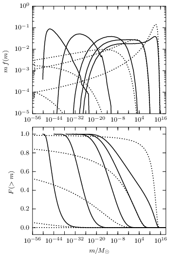
Examples of how the sub-halo ejection affects the halo mass function are shown in Fig. 4. In these calculations, the escape probability was assumed constant. Also the EPS mass function was used as the initial PDF. It is clearly seen that for larger escape probability $\chi_{\mathrm{ej}}$ the „tail“ of the low mass end (high $S$ values) of the mass function becomes heavier , i.e. the evolution of the population effectively slows down as $\chi_{\mathrm{ej}}$ increases.

In the kinetic approach presented above it is possible to use an appropriate arbitrary initial mass function. Thus, the problem of the choice of the initial conditions arises. According to the modern cosmological theory, matter-dominated era started at $z\approx 3\times 10^{3}$ [8]. According to the formal relation (21), structures with the variances $S\sim 10^{6}\dots 10^{7}$ or masses $\log(m/M_{\odot})\ll-100$ formed at that era (see Appendix). It is obvious, however, that the masses of the structures can not be lower than the mass of a hypothetical dark matter particle. If we take the value $m_{\mathrm{DM}}=100$ GeV $\sim 10^{-55}M_{\odot}$ as the mass of the dark matter particle (this value corresponds to $S_{\mathrm{DM}}\approx 10^{4}$), then the earliest structures may form at the redshifts as low as $z\sim 100$ (see Eq. (21)), and it is unlikely for structures to form at the higher redshifts. Finally, recalling the sub-halo escape model, we see that the sub-halos can not escape at the redshifts greater than $250$ (see Fig. 2). Considering all these restrictions, we assume the redshift value $z_{\mathrm{i}}\equiv 300$ as the initial moment for all calculations below. As the initial mass function we assume the cumulative distribution function

$$F(\omega_{\mathrm{i}},<S)=\left\{\begin{aligned} &F^{(0)}(\omega_{\mathrm{i}},<S)\;,\quad S\leqslant S_{\mathrm{DM}}\\ &1\;,\quad S>S_{\mathrm{DM}}\;,\end{aligned}\right.$$

(62)

where $\omega_{\mathrm{i}}=\delta_{\mathrm{c}}/D(z_{\mathrm{i}})$. Note that $F^{(0)}(\omega_{\mathrm{i}},<S_{\mathrm{DM}})\sim 10^{-7}$.

In Fig. 5 the mass functions in the model without sub-halo ejection ($\chi_{\mathrm{ej}}=0$) are plotted for the different redshifts. The initial mass function (62) peaks at the greater masses relatively to the peak of the EPS mass function (at $z=300$ the EPS peaks at $S\sim 10^{5}$), so the mass function at the subsequent times is also shifted to the higher masses. However, at $z\lesssim 15$ the massive end of the distribution coincides with the EPS model. In general, the low mass end of the mass function is suppressed at all redshifts, because of absence of the structures of mass $m_{\mathrm{DM}}$ and lower.

Obvious consequence of using the initial mass function suggested in this section is that the formation of the structures with masses lower than $m_{\mathrm{DM}}$ is impossible. This property may be used for the analysis of the resolution effects of cosmological codes built on top of the N-body or grid methods. The lowest possible mass scale in such applications should correspond to the spatial resolution of the numerical method.

Effect of the low density background structure (the supercluster or the void) can be considered in our model. Such a structure may be set in terms of the statistical constraints for the field of the overdensity fluctuations [12]. Applying the constraints leads to considerable change in statistics of modes of the fluctuations. E.g. the statistics is not more spatially uniform, the perturbations field „feels“ the size and shape of the background structure. Thus, the halo mass function also changes. In the EPS theory the effects of the background was considered first by Bond et al. [4], Bower [5], and investigated further by Mo and White [18], Sheth and Tormen [24] and others. When deviation of density of the background structure from uniform distribution is low, and the structure is large enough in all directions, the effect of the background presence can be accounted by a simple approach. Let’s denote $S_{\mathrm{B}}\equiv S(m_{\mathrm{B}})$ the variance of the overdensity fluctuations averaged over the background structure’s mass scale $m_{\mathrm{B}}$, then the variance of the field over the mass scale $m\ll m_{\mathrm{B}}$ placed deep inside the background structure is approximately $S(m)-S_{\mathrm{B}}$ [9, 12]. The same considerations are true for the velocity fluctuations field also (this fact was already utilized when the escape criterion (16) was obtained).

Bond et al. [4], Bower [5] have shown that the large scale background structure can be easily applied to the PS mass function Eq. (19) by formal substitutions of the kind

$$\omega\mapsto\omega-\omega_{\mathrm{B}}\;,\qquad S\mapsto S-S_{\mathrm{B}},$$

(63)

where $\omega_{\mathrm{B}}$ is the background overdensity calculated via the linear law (10), and reduced to the unit growth factor:

$$\omega_{\mathrm{B}}=\frac{D(z=0)}{D(z_{\mathrm{i}})}\,\Delta(z_{\mathrm{i}})=\frac{\delta_{\mathrm{c}}}{D(z_{\mathrm{f}})}\;.$$

(64)

The second equality in this expression allows to define an overdense structure which collapses by the moment $z_{\mathrm{f}}$. The equivalent description can be reached in the kinetic approach proposed in the previous section, if the substitutions (63) are made in the transfer PDF $f^{(0)}(\omega,S\,|\,\omega+\Delta\omega,S^{\prime})$.

The same substitutions may be utilized in the model with kinematic effects. It should be noted however, that the substitutions (63) must not be applied to escape probability $\chi_{\mathrm{ej}}(\omega,S,S^{\prime})$, because in fact the probability depends on the redshift and the halo mass, but not the overdensity threshold and the overdensity variance. Moreover, the velocity variance already enters Eq. (38), as the difference, hence its value, does not change as the velocity field varies, if these changes have the form (63). Finally, the transfer cross section is

$$q(\omega,S\,|\,\omega+\Delta\omega,S^{\prime})=[1-\chi_{\mathrm{ej}}(\omega,S,S^{\prime})]\,f^{(0)}(\omega-\omega_{\mathrm{B}},S-S_{\mathrm{B}}\,|\,\omega-\omega_{\mathrm{B}}+\Delta\omega,S^{\prime}-S_{\mathrm{B}})\;,$$

(65)

where $\omega_{\mathrm{B}}\equiv\delta_{\mathrm{B}}/D$. Note that the initial conditions (62) must not be transformed by (63).

References

- [1] LAMBDA – Legacy Archive for Microwave Background Data Analysis, 2013. URL http://lambda.gsfc.nasa.gov/.
- [2] J. M. Bardeen, J. R. Bond, N. Kaiser, and A. S. Szalay. The statistics of peaks of Gaussian random fields. ApJ, 304:15–61, May 1986. 10.1086/164143.
- [3] S. Bildhauer, T. Buchert, and M. Kasai. Solutions in Newtonian cosmology - The pancake theory with cosmological constant. A&A, 263:23–29, September 1992.
- [4] J. R. Bond, S. Cole, G. Efstathiou, and N. Kaiser. Excursion set mass functions for hierarchical Gaussian fluctuations. ApJ, 379:440–460, October 1991. 10.1086/170520.
- [5] R. G. Bower. The evolution of groups of galaxies in the Press-Schechter formalism. MNRAS, 248:332–352, January 1991.
- [6] M. Crocce and R. Scoccimarro. Renormalized cosmological perturbation theory. Phys. Rev. D, 73(6):063519–+, March 2006. 10.1103/PhysRevD.73.063519.
- [7] J. Diemand, M. Kuhlen, and P. Madau. Formation and Evolution of Galaxy Dark Matter Halos and Their Substructure. ApJ, 667:859–877, October 2007. 10.1086/520573.
- [8] D. S. Gorbunov and V. A. Rubakov. Introduction to the Theory of the Early Universe: Hot Big Bang Theory. World Scientific Publishing Co. Pte. Ltd., 5 Toh Tuck Link, Singapore 596224, 2011.
- [9] Y. Hoffman and E. Ribak. Constrained realizations of Gaussian fields - A simple algorithm. ApJ, 380:L5–L8, October 1991. 10.1086/186160.
- [10] M. J. Jee, R. L. White, N. Benítez, H. C. Ford, J. P. Blakeslee, P. Rosati, R. Demarco, and G. D. Illingworth. Weak-Lensing Analysis of the z˜=0.8 Cluster CL 0152-1357 with the Advanced Camera for Surveys. ApJ, 618:46–67, January 2005. 10.1086/425912.
- [11] I. D. Karachentsev, V. E. Karachentseva, and W. K. Huchtmeier. Disturbed isolated galaxies: indicators of a dark galaxy population? A&A, 451:817–820, June 2006. 10.1051/0004-6361:20054497.
- [12] E. P. Kurbatov. The mass function of dark halos in superclusters and voids. Astronomy Reports, 58:386–398, June 2014. 10.1134/S1063772914060031.
- [13] C. Lacey and S. Cole. Merger rates in hierarchical models of galaxy formation. MNRAS, 262:627–649, June 1993.
- [14] A. Lewis, A. Challinor, and A. Lasenby. Efficient Computation of Cosmic Microwave Background Anisotropies in Closed Friedmann-Robertson-Walker Models. ApJ, 538:473–476, August 2000. 10.1086/309179.
- [15] M. Maggiore and A. Riotto. The Halo Mass Function from Excursion Set Theory. I. Gaussian Fluctuations with Non-Markovian Dependence on the Smoothing Scale. ApJ, 711:907–927, March 2010a. 10.1088/0004-637X/711/2/907.
- [16] M. Maggiore and A. Riotto. The Halo mass function from Excursion Set Theory. II. The Diffusing Barrier. ApJ, 717:515–525, July 2010b. 10.1088/0004-637X/717/1/515.
- [17] D. Makarov and I. Karachentsev. Galaxy groups and clouds in the local () Universe. MNRAS, 412:2498–2520, April 2011. 10.1111/j.1365-2966.2010.18071.x.
- [18] H. J. Mo and S. D. M. White. An analytic model for the spatial clustering of dark matter haloes. MNRAS, 282:347–361, September 1996.
- [19] P. Natarajan and V. Springel. Abundance of Substructure in Clusters of Galaxies. ApJ, 617:L13–L16, December 2004. 10.1086/427079.
- [20] J. A. Peacock and A. F. Heavens. Alternatives to the Press-Schechter cosmological mass function. MNRAS, 243:133–143, March 1990.
- [21] P. J. E. Peebles. The large-scale structure of the universe. Princeton Univ. Press, Princeton, N.J., 1980.
- [22] Planck Collaboration, P. A. R. Ade, N. Aghanim, C. Armitage-Caplan, M. Arnaud, M. Ashdown, F. Atrio-Barandela, J. Aumont, C. Baccigalupi, A. J. Banday, and et al. Planck 2013 results. XVI. Cosmological parameters. ArXiv e-prints, March 2013.
- [23] W. H. Press and P. Schechter. Formation of Galaxies and Clusters of Galaxies by Self-Similar Gravitational Condensation. ApJ, 187:425–438, February 1974. 10.1086/152650.
- [24] R. K. Sheth and G. Tormen. Large-scale bias and the peak background split. MNRAS, 308:119–126, September 1999. 10.1046/j.1365-8711.1999.02692.x.
- [25] P. Valageas. Impact of a warm dark matter late-time velocity dispersion on large-scale structures. Phys. Rev. D, 86(12):123501, December 2012. 10.1103/PhysRevD.86.123501.