Optimal additive Schwarz methods for the $hp$ -BEM: the hypersingular integral operator in 3D on locally refined meshes

T. Führer Email: tofuhrer@mat.puc.cl Address: Pontificia Universidad Católica de Chile, Facultad de Matemáticas, Vicuña Mackenna 4860, Santiago, Chile. J. M. Melenk Email: melenk@tuwien.ac.at Address: Technische Universität Wien, Institut für Analysis und Scientific Computing, Wiedner Hauptstraße 8-10, A-1040 Vienna Corresponding author: Corresponding author D. Praetorius Email: dirk.praetorius@tuwien.ac.at Address: Technische Universität Wien, Institut für Analysis und Scientific Computing, Wiedner Hauptstraße 8-10, A-1040 Vienna A. Rieder Email: alexander.rieder@tuwien.ac.at Address: Technische Universität Wien, Institut für Analysis und Scientific Computing, Wiedner Hauptstraße 8-10, A-1040 Vienna

August 24, 2026

Abstract

We propose and analyze an overlapping Schwarz preconditioner for the $p$ and $hp$ boundary element method for the hypersingular integral equation in 3D. We consider surface triangulations consisting of triangles. The condition number is bounded uniformly in the mesh size $h$ and the polynomial order $p$ . The preconditioner handles adaptively refined meshes and is based on a local multilevel preconditioner for the lowest order space. Numerical experiments on different geometries illustrate its robustness.

Keywords:

hp

-BEM, hypersingular integral equation, preconditioning, additive Schwarz method

MSC

65N35, 65N38, 65N55

1 Introduction

Many elliptic boundary value problems that are solved in practice are linear and have constant (or at least piecewise constant) coefficients. In this setting, the boundary element method (BEM, [21, 35, 39, 31]) has established itself as an effective alternative to the finite element method (FEM). Just as in the FEM applied to this particular problem class, high order methods are very attractive since they can produce rapidly convergent schemes on suitably chosen adaptive meshes. The discretization leads to large systems of equations, and a use of iterative solvers brings the question of preconditioning to the fore.

In the present work, we study high order Galerkin discretizations of the hypersingular operator. This is an operator of order $1$ , and we therefore have to expect the condition number of the system matrix to increase as the mesh size $h$ decreases and the approximation order $p$ increases. We present an additive overlapping Schwarz preconditioner that offsets this degradation and results in condition numbers that are bounded independently of the mesh size and the approximation order. This is achieved by combining the recent $H^{1/2}$ -stable decomposition of spaces of piecewise polynomials of degree $p$ of [23] and the multilevel diagonal scaling preconditioner of [14, 16] for the hypersingular operator discretized by piecewise linears.

Our additive Schwarz preconditioner is based on stably decomposing the approximation space of piecewise polynomials into the lowest order space (i.e., piecewise linears) and spaces of higher order polynomials supported by the vertex patches. Such stable localization procedures were first developed for the $hp$ -FEM in [34] for meshes consisting of quadrilaterals (or, more generally, tensor product elements). The restriction to tensor product elements stems from the fact that the localization is achieved by exploiting stability properties of the 1D-Gauß-Lobatto interpolation operator, which, when applied to polynomials, is simultaneously stable in $L^{2}$ and $H^{1}$ (see, e.g., [7, eqns. (13.27), (13.28)]). This simultaneous stability raises the hope for $H^{1/2}$ -stable localizations and was pioneered in [18] for the $hp$ -BEM for the hypersingular operator on meshes consisting of quadrilaterals. Returning to the $hp$ -FEM, $H^{1}$ -stable localizations on triangular/tetrahedral meshes were not developed until [36]. The techniques developed there were subsequently used in [23] to design $H^{1/2}$ -stable decompositions on triangular meshes and thus paved the way for condition number estimates that are uniform in the approximation $p$ for overlapping Schwarz methods for the $hp$ -version BEM applied to the hypersingular operator. Non-overlapping additive Schwarz preconditioners for high order discretizations of the hypersingular operator are also available in the literature, [1]; as it is typical of this class of preconditioners, the condition number still grows polylogarithmically in $p$ .

Our preconditioner is based on decomposing the approximation space into the space of piecewise linears and spaces associated with the vertex patches. It is highly desirable to decompose the space of piecewise linears further in a multilevel fashion. For sequences of uniformly refined meshes, the first such multilevel space decomposition appears to be [43] (see also [33]). For adaptive meshes, local multilevel diagonal scaling was first analyzed in [2], where for a sequence $\mathcal{T}_{\ell}$ of successively refined adaptive meshes a uniformly bounded condition number for the preconditioned system is established. Formally, however, [2] requires that $\mathcal{T}_{\ell}\cap\mathcal{T}_{\ell+1}\subset\mathcal{T}_{\ell+k}$ for all $\ell,k\in\mathbb{N}_{0}$ , i.e., as soon as an element $K\in\mathcal{T}_{\ell}$ is not refined, it remains non-refined in all succeeding triangulations. While this can be achieved implementationally, the recent works [14, 16] avoid such a restriction by considering sequences of meshes that are obtained in typical $h$ -adaptive environments with the aid of newest vertex bisection (NVB). We finally note that the additive Schwarz decomposition on adaptively refined meshes is a subtle issue. Hierarchical basis preconditioners (which are based on the new nodes only) lead to a growth of the condition number with $\mathcal{O}(\left|\log{h_{min}}\right|^{2})$ ; see [44]. Global multilevel diagonal preconditioning (which is based on all nodes) leads to a growth $\mathcal{O}(\left|\log{h_{min}}\right|)$ ; see [28, 14].

The paper is organized as follows: In Section 2 we introduce the hypersingular equation and the discretization by high order piecewise polynomial spaces. Section 3 collects properties of the fractional Sobolev spaces including the scaling properties. Section 4 studies in detail the $p$ -dependence of the condition number of the unpreconditioned system. The polynomial basis on the reference triangle chosen by us is a hierarchical basis of the form first proposed by Karniadakis & Sherwin, [25, Appendix D.1.1.2]; the precise form is the one from [50, Section 5.2.3]. We prove bounds for the condition number of the stiffness matrix not only in the $H^{1/2}$ -norm but also in the norms of $L^{2}$ and $H^{1}$ . This is also of interest for $hp$ -FEM and could not be found in the literature. Section 5 develops several preconditioners. The first one (Theorem 5.3) is based on decomposing the high order approximation space into the global space of piecewise linears and local high order spaces of functions associated with the vertex patches. The second one (Theorem 5.6) is based on a further multilevel decomposition of the global space of piecewise linears. The third one (Theorem 5.10) exploits the observation that topologically, only a finite number of vertex patches can occur. Hence, significant memory savings for the preconditioner are possible if the exact bilinear forms for the vertex patches are replaced with scaled versions of simpler ones defined on a finite number of reference configurations. Numerical experiments in Section 6 illustrate that the proposed preconditioners are indeed robust with respect to both $h$ and $p$ .

We close with a remark on notation: The expression $a\lesssim b$ signifies the existence of a constant $C>0$ such that $a\leq C\,b$ . The constant $C$ does not depend on the mesh size $h$ and the approximation order $p$ , but may depend on the geometry and the shape regularity of the triangulation. We also write $a\sim b$ to abbreviate $a\lesssim b\lesssim a$ .

2 $hp$ -discretization of the hypersingular integral equation

2.1 Hypersingular integral equation

Let $\Omega\subset\mathbb{R}^{3}$ be a bounded Lipschitz polyhedron with a connected boundary $\partial\Omega$ , and let $\Gamma\subseteq\partial\Omega$ be an open, connected subset of $\partial\Omega$ . If $\Gamma\neq\partial\Omega$ , we assume it to be a Lipschitz hypograph, [31]; the key property needed is that $\Gamma$ is such that the ellipticity condition (2.2) holds. Furthermore, we will use affine, shape regular triangulations of $\Gamma$ , which further imposes conditions on $\Gamma$ . In this work, we are concerned with preconditioning high order discretizations of the hypersingular integral operator, which is given by

\displaystyle\left(Du\right)(x)

\displaystyle:=-\partial_{n_{x}}^{int}\int_{\Gamma}{\partial_{n_{y}}^{int}G(x,y)u(y)\;ds_{y}}\quad\text{for }x\in\Gamma,

(2.1)

where $G(x,y):=\frac{1}{4\pi}\frac{1}{\left|x-y\right|}$ is the fundamental solution of the 3D-Laplacian and $\partial_{n_{y}}^{int}$ denotes the (interior) normal derivative with respect to $y\in\Gamma$ .

We will need some results from the theory of Sobolev and interpolation spaces, see [31, Appendix B]. For an open subset $\omega\subset\partial\Omega$ , let $L^{2}(\omega)$ and $H^{1}(\omega)$ denote the usual Sobolev spaces. The space $\widetilde{H}^{1}(\omega)$ consists of those functions whose zero extension to $\partial\Omega$ is in $H^{1}(\partial\Omega)$ . (In particular, for $\omega=\partial\Omega$ , $H^{1}(\partial\Omega)=\widetilde{H}^{1}(\partial\Omega)$ .) When the surface measure of the set $\partial\Omega\setminus\omega$ is positive, we use the equivalent norm $\left\|u\right\|_{\widetilde{H}^{1}(\omega)}^{2}:=\left\|\nabla_{\Gamma}u\right\|^{2}_{L^{2}(\omega)}$ .

We will define fractional Sobolev norms by interpolation. The following Proposition 2.1 collects key properties of interpolation spaces that we will need; we refer to [41, 45] for a comprehensive treatment. For two Banach spaces $\left(X_{0},\left\|\cdot\right\|_{0}\right)$ and $\left(X_{1},\left\|\cdot\right\|_{1}\right)$ , with continuous inclusion $X_{1}\subseteq X_{0}$ and a parameter $s\in(0,1)$ the interpolation norm is defined as

\displaystyle\left\|u\right\|^{2}_{[X_{0},X_{1}]_{s}}

\displaystyle:=\int_{t=0}^{\infty}t^{-2s}\left(\inf_{v\in X_{1}}\|u-v\|_{0}+t\|v\|_{1}\right)^{2}\frac{dt}{t}.

The interpolation space is given by $\left[X_{0},X_{1}\right]_{s}:=\left\{u\in X_{0}:\left\|u\right\|_{[X_{0},X_{1}]_{s}}<\infty\right\}$ .

An important result, which we use in this paper, is the following interpolation theorem:

Proposition 2.1.

Let $X_{i}$ , $Y_{i}$ , $i\in\{0,1\}$ , be two pairs of Banach spaces with continuous inclusions $X_{1}\subseteq X_{0}$ and $Y_{1}\subseteq Y_{0}$ . Let $s\in(0,1)$ .

(i)

If a linear operator $T$ is bounded as an operator $X_{0}\to Y_{0}$ and $X_{1}\to Y_{1}$ , then it is also bounded as an operator $[X_{0},X_{1}]_{s}\to[Y_{0},Y_{1}]_{s}$ with

\displaystyle\left\|T\right\|_{[X_{0},X_{1}]_{s}\to[Y_{0},Y_{1}]_{s}}\leq\left\|T\right\|_{X_{0}\to Y_{0}}^{1-s}\left\|T\right\|_{X_{1}\to Y_{1}}^{s}.

(ii)

There exists a constant $C>0$ such that for all $x\in X_{1}$ : $\displaystyle\left\|x\right\|_{[X_{0},X_{1}]_{s}}\leq C\left\|x\right\|_{X_{0}}^{1-s}\left\|x\right\|_{X_{1}}^{s}.$

We define the fractional Sobolev spaces by interpolation. For $s\in(0,1)$ , we set:

\displaystyle H^{s}(\omega)

\displaystyle:=\left[L^{2}(\omega),H^{1}(\omega)\right]_{s},\quad\widetilde{H}^{s}(\omega):=\left[L^{2}(\omega),\widetilde{H}^{1}(\omega)\right]_{s}.

Here, we will only consider the case $s=1/2$ . We define $H^{-1/2}(\Gamma)$ as the dual space of $\widetilde{H}^{1/2}(\Gamma)$ , where duality is understood with respect to the (continuously) extended $L^{2}(\Gamma)$ -scalar product and denoted by $\left<\cdot,\cdot\right>_{\Gamma}$ . An equivalent norm on $H^{1/2}(\Gamma)$ is given by ${\left\|u\right\|_{H^{1/2}(\Gamma)}^{2}\sim\left\|u\right\|_{L^{2}(\Gamma)}^{2}+\left|u\right|_{H^{1/2}(\Gamma)}^{2}}$ , where $\left|\cdot\right|_{H^{1/2}(\Gamma)}$ is given by the Sobolev-Slobodeckij seminorm (see [35] for the exact definition).

We now state some important properties of the hypersingular operator $D$ from (2.1), see, e.g., [35, 31, 21, 39]. First, the operator $D:\widetilde{H}^{1/2}(\Gamma)\to H^{-1/2}(\Gamma)$ is a bounded linear operator.

For open surfaces $\Gamma\subsetneqq\partial\Omega$ the operator is elliptic

\displaystyle\left<Du,u\right>_{\Gamma}

\displaystyle\geq c_{ell}\left\|u\right\|_{\widetilde{H}^{1/2}(\Gamma)}^{2}\quad\quad\forall u\in\widetilde{H}^{1/2}(\Gamma),

(2.2)

with some constant $c_{ell}>0$ that only depends on $\Gamma$ . In the case of a closed surface, i.e. $\Gamma=\partial\Omega$ we note that $\widetilde{H}^{1/2}(\Gamma)=H^{1/2}(\Gamma)$ and the operator $D$ is still semi-elliptic, i.e.

\displaystyle\left<Du,u\right>_{\Gamma}

\displaystyle\geq c_{ell}\left|u\right|_{H^{1/2}(\Gamma)}^{2}\quad\quad\forall u\in\widetilde{H}^{1/2}(\Gamma).

Moreover, the kernel of $D$ then consists of the constant functions only: $\operatorname{ker}(D)\penalty\ =\penalty\ \operatorname{span}(1)$ .

To get unique solvability and strong ellipticity for the case of a closed surface, it is customary to introduce a stabilized operator $\widetilde{D}$ given by the bilinear form

\displaystyle\left<\widetilde{D}u,v\right>_{\Gamma}:=\left<Du,v\right>_{\Gamma}+\alpha^{2}\left<u,1\right>_{\Gamma}\left<v,1\right>_{\Gamma},\quad\alpha>0.

(2.3)

In order to avoid having to distinguish the two cases $\Gamma=\partial\Omega$ and $\Gamma\subsetneqq\partial\Omega$ , we will only work with the stabilized form on $\widetilde{H}^{1/2}(\Gamma)$ and just set $\alpha=0$ in the case of $\Gamma\subsetneqq\partial\Omega$ . The basic integral equation involving the hypersingular operator $D$ then reads: For given $g\in H^{-1/2}(\Gamma)$ , find $u\in\widetilde{H}^{1/2}(\Gamma)$ such that

\displaystyle\left<\widetilde{D}u,v\right>_{\Gamma}

\displaystyle=\left<g,v\right>_{\Gamma}\quad\forall v\in\widetilde{H}^{1/2}(\Gamma).

(2.4)

We note that in the case of the closed surface $\Gamma=\partial\Omega$ , the solution of the stabilized system above is equivalent to the solution of $\left<Du,v\right>_{\Gamma}=\left<g,v\right>_{\Gamma}$ under the side constraint $\left<u,1\right>_{\Gamma}=\frac{\left<g,1\right>_{\Gamma}}{\alpha^{2}\,\left|\Gamma\right|}$ . Moreover, it is well known that $\left<\widetilde{D}\cdot,\cdot\right>_{\Gamma}$ is symmetric, elliptic and induces an equivalent norm on $\widetilde{H}^{1/2}(\Gamma)$ , i.e.,

\displaystyle\left<\widetilde{D}u,u\right>_{\Gamma}\sim\left\|u\right\|_{\widetilde{H}^{1/2}(\Gamma)}^{2}\quad\quad\forall u\in\widetilde{H}^{1/2}(\Gamma).

2.2 Discretization

Let $\mathcal{T}=\{K_{1},\dots,K_{N}\}$ denote a regular (in the sense of Ciarlet) triangulation of the two-dimensional manifold $\Gamma\subseteq\partial\Omega$ into compact, non-degenerate planar surface triangles. We say that a triangulation is $\gamma$ -shape regular, if there exists a constant $\gamma>0$ such that

\displaystyle\max_{K\in\mathcal{T}}\frac{\mathrm{diam}(K)^{2}}{|K|}\leq\gamma.

(2.5)

Let $\widehat{K}:=\operatorname{conv}\{(0,0),(1,0),(0,1)\}$ be the reference triangle. With each element $K$ we associate an affine, bijective element map $F_{K}:\widehat{K}\to K$ . We will write $P^{p}(\widehat{K})$ for the space of polynomials of degree $p$ on $\widehat{K}$ . The space of piecewise polynomials on $\mathcal{T}$ is given by

\displaystyle P^{p}(\mathcal{T}):=\left\{u\in L^{2}(\Gamma)\,:\,u\circ F_{K}\in P^{p}(\widehat{K})\text{ for all }K\in\mathcal{T}\right\}.

(2.6)

The elementwise constant mesh width function $h:=h_{\mathcal{T}}\in P^{0}(\mathcal{T})$ is defined by $(h_{\mathcal{T}})|_{K}:=\mathrm{diam}(K)$ for all $K\in\mathcal{T}$ .

Let ${\mathcal{V}}=\{{\boldsymbol{z}}_{1},\dots,{\boldsymbol{z}}_{M}\}$ denote the set of all vertices of the triangulation $\mathcal{T}$ that are not on the boundary of $\Gamma$ . We define the (vertex) patch $\omega_{\boldsymbol{z}}$ for a vertex ${\boldsymbol{z}}\in{\mathcal{V}}$ by

\displaystyle\omega_{\boldsymbol{z}}:=\operatorname*{interior}\left(\bigcup_{\left\{K\in\mathcal{T}:\;{\boldsymbol{z}}\in K\right\}}K\right),

(2.7)

where the interior is understood with respect to the topology of $\Gamma$ . For $p\geq 1$ , define

\displaystyle\widetilde{S}^{p}(\mathcal{T}):=P^{p}(\mathcal{T})\cap\widetilde{H}^{1/2}(\Gamma).

(2.8)

Then, the Galerkin discretization of (2.4) consists in replacing $\widetilde{H}^{1/2}(\Gamma)$ with the discrete subspace $\widetilde{S}^{p}(\mathcal{T})$ , i.e.: Find $u_{h}\in\widetilde{S}^{p}(\mathcal{T})$ such that

\displaystyle\left<\widetilde{D}u_{h},v_{h}\right>_{\Gamma}=\left<g,v_{h}\right>_{\Gamma}\quad\text{for all }v_{h}\in\widetilde{S}^{p}(\mathcal{T}).

(2.9)

Remark 2.2.

We employ the same polynomial degree for all elements. This is not essential and done for simplicity of presentation. For details on the more general case, see [23].

After choosing a basis of $\widetilde{S}^{p}(\mathcal{T})$ , the problem (2.9) can be written as a linear system of equations, and we write $\widetilde{D}^{p}_{h}$ for the resulting system matrix. Our goal is to construct a preconditioner for $\widetilde{D}^{p}_{h}$ . It is well-known that the condition number of $\widetilde{D}_{h}^{p}$ depends on the choice of the basis of $\widetilde{S}^{p}(\mathcal{T})$ , which we fix in Definition 2.4 below. We remark in passing that the preconditioned system of Section 5.2 will no longer depend on the basis.

2.3 Polynomial basis on the reference element

For the matrix representation of the Galerkin formulation (2.9) we have to specify a polynomial basis on the reference triangle $\widehat{K}$ . We use a basis that relies on a collapsed tensor product representation of the triangle and is given in [50, Section 5.2.3]. This kind of basis was first proposed for the $hp$ -FEM by Karniadakis & Sherwin, [25, Appendix D.1.1.2]; closely related earlier works on polynomial bases that rely on a collapsed tensor product representation of the triangle are [26, 9].

Definition 2.3 (Jacobi polynomials).

For coefficients $\alpha$ , $\beta>-1$ the family of Jacobi polynomials on the interval $\left(-1,1\right)$ is denoted by $P_{n}^{(\alpha,\beta)}$ , $n\in\mathbb{N}_{0}$ . They are orthogonal with respect to the $L^{2}(-1,1)$ inner product with weight $(1-x)^{\alpha}(1+x)^{\beta}$ . (See for example [25, Appendix A] or [50, Appendix A.3] for the exact definitions and a list of important properties). The Legendre polynomials are a special case of the Jacobi polynomials for $\alpha=\beta=0$ and denoted by $\ell_{n}(s):=P^{(0,0)}_{n}(s)$ . The integrated Legendre polynomials $L_{n}$ and the scaled polynomials are defined by

\displaystyle L_{n}(s)

\displaystyle:=\int_{-1}^{s}{\ell_{n-1}(t)dt}\quad\text{for }n\in\mathbb{N},

\displaystyle P_{n}^{\mathcal{S},(\alpha,\beta)}(s,t)

\displaystyle:=t^{n}P^{(\alpha,\beta)}_{n}(s/t),

\displaystyle L_{n}^{\mathcal{S}}(s,t)

\displaystyle:=t^{n}L_{n}(s/t).

(2.10)

On the reference triangle, our basis reads as follows:

Definition 2.4 (polynomial basis on the reference triangle).

Let $p\in{\mathbb{N}}$ and let $\lambda_{1},\lambda_{2},\lambda_{3}$ be the barycentric coordinates on the reference triangle $\widehat{K}$ . Then the basis functions for the reference triangle consist of three vertex functions, $p-1$ edge functions per edge, and $(p-1)(p-2)/2$ cell-based functions:

(a)

for $i=1$ , $2$ , $3$ the vertex functions are:

	$\displaystyle\varphi^{\mathcal{V}}_{i}$	$\displaystyle:=\lambda_{i};$
	(b) for $m=1$ , $2$ , $3$ and an edge $\mathcal{E}_{m}$ with edge vertices $e_{1},e_{2}$ , the edge functions are given by:
	$\displaystyle\varphi_{i}^{\mathcal{E}_{m}}$	$\displaystyle:=\sqrt{\frac{2i+3}{2}}\,L_{i+2}^{\mathcal{S}}(\lambda_{e_{2}}-\lambda_{e_{1}},\lambda_{e_{1}}+\lambda_{e_{2}}),\quad\quad 0\leq i\leq p-2;$
	(c) for $0\leq i+j\leq p-3$ the cell based functions are:
	$\displaystyle\varphi_{(i,j)}^{\mathcal{I}}$	$\displaystyle:=c_{ij}\lambda_{1}\lambda_{2}\lambda_{3}P_{i}^{\mathcal{S},(2,2)}(\lambda_{1}-\lambda_{2},\lambda_{1}+\lambda_{2})\,P_{j}^{(2i+5,2)}(2\lambda_{3}-1).$

with $c_{ij}$ such that $\left\|\varphi_{(i.j)}^{\mathcal{I}}\right\|_{L^{2}(\widehat{K})}=1$ .

Remark 2.5.

In order to get a basis of $\widetilde{S}^{p}(\mathcal{T})$ we take the composition with the element mappings $\varphi\circ F_{K}$ . To ensure continuity along edges we take an arbitrary orientation of the edges and observe that the edge basis functions $\varphi_{i}^{\mathcal{E}}$ are symmetric under permutation of $\lambda_{e_{1}}$ and $\lambda_{e_{2}}$ up to a sign change $(-1)^{i}$ .

3 Properties of $\widetilde{H}^{1/2}(\Gamma)$

3.1 Quasi-interpolation in $\widetilde{H}^{1/2}(\Gamma)$

Several results of the present paper depend on results in [23]. Therefore we present a short summary of the main results of that paper in this section. In [23] the authors propose an $H^{1/2}$ -stable space decomposition on meshes consisting of triangles. It is based on quasi-interpolation operators constructed by local averaging on elements.

We introduce the following product spaces:

\displaystyle X_{0}

\displaystyle:=\prod_{\boldsymbol{z}\in{\mathcal{V}}}{L^{2}(\omega_{\boldsymbol{z}})},\quad\quad X_{1}:=\prod_{\boldsymbol{z}\in{\mathcal{V}}}{\widetilde{H}^{1}(\omega_{\boldsymbol{z}})}.

The spaces $L^{2}(\omega_{\boldsymbol{z}})$ and $\widetilde{H}^{1}(\omega_{\boldsymbol{z}})$ are endowed with the $L^{2}$ - and $\widetilde{H}^{1}$ -norm, respectively.

Proposition 3.1 (localization, [23]).

There exists an operator $J:L^{2}(\Gamma)\to\left(\widetilde{\mathcal{S}}^{1}(\mathcal{T}),\left\|\cdot\right\|_{L^{2}(\Gamma)}\right)\times X_{0}$ with the following properties:

(i)

$J$ is linear and bounded.
(ii)

$J|_{\widetilde{H}^{1}(\Gamma)}$ is also bounded as an operator $\widetilde{H}^{1}(\Gamma)\to\left(\widetilde{\mathcal{S}}^{1}(\mathcal{T}),\left\|\cdot\right\|_{\widetilde{H}^{1}(\Gamma)}\right)\times X_{1}$ .
(iii)

If $u\in\widetilde{S}^{p}(\mathcal{T})$ then each component of $Ju$ is in $\widetilde{S}^{p}(\mathcal{T})$ .

(iv)

If we write $Ju=:(u_{1},U)$ , and furthermore $U_{\boldsymbol{z}}$ for the component of $U$ in $X_{0}$ corresponding to the space $L^{2}(\omega_{\boldsymbol{z}})$ , then $Ju$ represents an $\widetilde{H}^{1/2}(\Gamma)-stable$ decomposition of $u$ , i.e.,

\displaystyle u

\displaystyle=u_{1}+\sum_{\boldsymbol{z}\in{\mathcal{V}}}{U_{\boldsymbol{z}}}\quad\text{and}\quad\left\|u_{1}\right\|_{\widetilde{H}^{1/2}(\Gamma)}^{2}+\sum_{\boldsymbol{z}\in{\mathcal{V}}}{\left\|U_{\boldsymbol{z}}\right\|_{\widetilde{H}^{1/2}(\omega_{\boldsymbol{z}})}^{2}}\leq C\left\|u\right\|_{\widetilde{H}^{1/2}(\Gamma)}^{2}.

(3.1)

The norms of $J$ in (i)—(ii) and the constant $C>0$ in (iv) depend only on $\Gamma$ and the shape regularity constant $\gamma$ .

Sketch of proof: .

The first component of $J$ (i.e., the mapping $u\mapsto u_{1}$ ) consists of the Scott-Zhang projection operator, as modified in [3, Section 3.2]. The local components (i.e., the functions $U_{\boldsymbol{z}}$ , $z\in{\mathcal{V}}$ ) then are based on a successive decomposition into vertex, edge and interior parts, similar to what is done in [36]. We give a flavor of the procedure. Set $u_{2}:=u-u_{1}$ . In order to define the vertex parts for a vertex $\boldsymbol{z}$ , we select an element $K\subset\omega_{\boldsymbol{z}}$ of the patch $\omega_{\boldsymbol{z}}$ and perform a suitable local averaging of $u_{2}$ on that element; this averaged function $u_{loc,K}$ is defined on $K$ in terms of $u_{2}|_{K}$ and vanishes on the edge opposite $\boldsymbol{z}$ . In order to extend $u_{loc,K}$ to the patch $\omega_{\boldsymbol{z}}$ and thus obtain the function $u_{\boldsymbol{z}}$ , we define $u_{\boldsymbol{z}}$ by “rotating” $u_{loc,K}$ around the vertex $\boldsymbol{z}$ . The averaging process can be done in such a way that for continuous functions $u_{2}$ one has $u_{2}(\boldsymbol{z})=u_{\boldsymbol{z}}(\boldsymbol{z})$ and that one has appropriate stability properties in $L^{2}$ and $H^{1}$ . The edge contributions are constructed from the function $u_{3}:=u_{2}-\sum_{\boldsymbol{z}\in{\mathcal{V}}}u_{\boldsymbol{z}}$ . Let ${\mathcal{E}}(\mathcal{T})$ denote the set of interior edges of $\mathcal{T}$ . For an edge ${\mathcal{E}}\in{\mathcal{E}}(\mathcal{T})$ one selects an element (of which ${\mathcal{E}}$ is an edge), averages there, and extends the obtained averaged function to the edge patch by symmetry across the edge ${\mathcal{E}}$ . In this way, the function $u_{{\mathcal{E}}}$ is constructed for each edge ${\mathcal{E}}$ . It again holds for sufficiently smooth $u_{3}$ that $u_{3}(x)=u_{{\mathcal{E}}}(x)\;\forall x\in{\mathcal{E}}$ . For $u\in\widetilde{H}^{1}(\Gamma)$ and in turn $u_{2}\in\widetilde{H}^{1}(\Gamma)$ , we have that $u_{4}:=u-\sum_{{\mathcal{E}}\in\mathcal{E}(\mathcal{T})}{u_{\mathcal{E}}}-\sum_{\boldsymbol{z}\in{\mathcal{V}}}{u_{\boldsymbol{z}}}$ vanishes on all edges; hence $u_{4}|_{K}\in\widetilde{H}^{1}(K)$ for all $K\in\mathcal{T}$ . The terms $u_{\boldsymbol{z}}$ , $u_{\mathcal{E}}$ , $u_{4}|_{K}$ can be rearranged to take the form of patch contributions $U_{\boldsymbol{z}}$ as given in the statement of the proposition. (The decomposition is not unique.) The $\widetilde{H}^{1/2}$ stability is a direct consequence of the $L^{2}$ and $H^{1}$ stability and interpolation properties given in Proposition 2.1, (i). We finally mention that assertion (iii) follows from the fact that the averaging operators employed at the various stages of the decomposition are polynomial preserving. ∎

Remark 3.2.

Independently, a decomposition similar to Proposition 3.1 was presented in [10].

The construction in Proposition 3.1 can be modified and used to relate the $\widetilde{H}^{1/2}(\omega_{\boldsymbol{z}})$ -norm to the $\widetilde{H}^{1/2}({\mathcal{O}})$ -norm if ${\mathcal{O}}\supset\omega_{\boldsymbol{z}}$ :

Corollary 3.3.

Let $\boldsymbol{z}\in{\mathcal{V}}$ and $\mathcal{O}$ be the union of some triangles of $\mathcal{T}$ with $\omega_{\boldsymbol{z}}\subseteq\mathcal{O}\subseteq\Gamma$ . Then there exist constants $c_{1},c_{2}$ that depend only on $\mathcal{O}$ , $\Gamma$ , and the $\gamma$ -shape regularity of $\mathcal{T}$ such that for all $u\in\widetilde{H}^{1/2}(\mathcal{O})$ with $\operatorname{supp}(u)\subseteq\overline{\omega_{\boldsymbol{z}}}$ , we can estimate:

\displaystyle c_{1}\;\left\|u\right\|_{\widetilde{H}^{1/2}(\omega_{\boldsymbol{z}})}

\displaystyle\leq\left\|u\right\|_{\widetilde{H}^{1/2}(\mathcal{O})}\leq c_{2}\left\|u\right\|_{\widetilde{H}^{1/2}(\omega_{\boldsymbol{z}})}.

Proof.

To see the second inequality, consider the extension operator $E$ that extends the function $u$ by $0$ outside of $\omega_{\boldsymbol{z}}$ . This operator is continuous $L^{2}(\omega_{\boldsymbol{z}})\rightarrow L^{2}(\mathcal{O})$ and $\widetilde{H}^{1}(\omega_{\boldsymbol{z}})\rightarrow\widetilde{H}^{1}(\mathcal{O})$ , both with constant $1$ . Applying Proposition 2.1, (i) to this extension operator $E$ gives the second inequality with $c_{2}=1$ . The first inequality is more involved. We start by noting that the stability assertion (3.1) of Proposition 3.1 gives $u=u_{1}+\sum_{\boldsymbol{z^{\prime}}\in{\mathcal{V}}}U_{\boldsymbol{z^{\prime}}}$ and

\displaystyle\left\|u_{1}\right\|^{2}_{\widetilde{H}^{1/2}(\mathcal{O})}+\sum_{\boldsymbol{z^{\prime}}\in{\mathcal{V}}}{\left\|U_{\boldsymbol{z^{\prime}}}\right\|^{2}_{\widetilde{H}^{1/2}(\omega_{\boldsymbol{z^{\prime}}})}}

\displaystyle\leq C\left\|u\right\|^{2}_{\widetilde{H}^{1/2}(\mathcal{O})}.

(3.2)

The constant $C$ depends only on the set ${\mathcal{O}}$ and the shape regularity of the triangulation, when Proposition 3.1 is applied with $\Gamma$ replaced by $\mathcal{O}$ . The decomposition in Proposition 3.1 is not unique, and we will now exploit this by requiring more. Specifically, we assert that the operator $J$ , which effects the decomposition, can be chosen such that, for given $\omega_{\boldsymbol{z}}$ , we have $\operatorname*{supp}u_{1}\subset\overline{\omega_{\boldsymbol{z}}}$ and $U_{\boldsymbol{z}^{\prime}}=0$ for $\boldsymbol{z}^{\prime}\neq\boldsymbol{z}$ . If this can be achieved, we get $u=u_{1}+U_{\boldsymbol{z}}$ . Since (3.2) contains a term $\left\|u_{1}\right\|_{\widetilde{H}^{1/2}(\mathcal{O})}$ , we also need to reinvestigate the stability proof. The decomposition is $L^{2}$ - and $H^{1}$ -stable, and maps to functions with $\operatorname*{supp}u_{1}\subset\overline{\omega_{\boldsymbol{z}}}$ . Therefore, we can interpret the first component of $J$ as an operator mapping to $\widetilde{H}^{1}(\omega_{\boldsymbol{z}})$ and apply Proposition 2.1 (i) to get:

\left\|u_{1}\right\|_{\widetilde{H}^{1/2}(\omega_{\boldsymbol{z}})}+\left\|U_{\boldsymbol{z}}\right\|_{\widetilde{H}^{1/2}(\omega_{\boldsymbol{z}})}\leq C\left\|u\right\|_{\widetilde{H}^{1/2}(\mathcal{O})}.

The triangle inequality $\left\|u\right\|_{\widetilde{H}^{1/2}(\omega_{\boldsymbol{z}})}\leq\left\|u_{1}\right\|_{\widetilde{H}^{1/2}(\omega_{\boldsymbol{z}})}+\left\|U_{\boldsymbol{z}}\right\|_{\widetilde{H}^{1/2}(\omega_{\boldsymbol{z}})}$ then concludes the proof.

It therefore remains to see that we can construct the operator $J$ of Proposition 3.1 with the additional property that $u=u_{1}+U_{\boldsymbol{z}}$ if $u$ is such that $\operatorname*{supp}u\subset\overline{\omega_{\boldsymbol{z}}}$ . This follows by carefully selecting the elements on which the local averaging is done, namely, whenever one has to choose an element on which to average, one selects, if possible, an element that is not contained in $\omega_{\boldsymbol{z}}$ . For example for vertex contributions $\boldsymbol{z^{\prime}}\in\partial\omega_{\boldsymbol{z}}$ we make sure to use elements $K^{\prime}$ which are not in $\omega_{\boldsymbol{z}}$ . This implies that for $\operatorname{supp}(u)\subseteq\overline{\omega_{\boldsymbol{z}}}$ we get $u_{\boldsymbol{z^{\prime}}}=0$ . A similar choice is made when defining the edge contributions. ∎

The stable space decomposition of Proposition 3.1 is one of several ingredients of the proof that the interpolation space obtained by interpolating the space $\widetilde{S}^{p}(\mathcal{T})$ endowed with the $L^{2}$ -norm and the $H^{1}$ -norm yields the space $\widetilde{S}^{p}(\mathcal{T})$ endowed with the appropriate fractional Sobolev norm:

Proposition 3.4 ([23]).

Let $s\in(0,1)$ and let $\mathcal{T}$ be a shape regular triangulation of $\Gamma$ . Let $p\geq 1$ . Then:

\displaystyle\left[\left(\widetilde{S}^{p}(\mathcal{T}),\left\|\cdot\right\|_{L^{2}(\Gamma)}\right),\left(\widetilde{S}^{p}(\mathcal{T}),\left\|\cdot\right\|_{\widetilde{H}^{1}(\Gamma)}\right)\right]_{s}

\displaystyle=\left(\widetilde{S}^{p}(\mathcal{T}),\left\|\cdot\right\|_{\widetilde{H}^{s}(\Gamma)}\right).

The constants implied in the norm equivalence depend only on $\Gamma$ , $s$ , and the $\gamma$ -shape regularity of $\mathcal{T}$ .

We note that such a result is clearly valid for fixed $p\geq 1$ (see, e.g., [3, Proof of Prop. 5]), but the essential observation of [23] is that the norm equivalence constants do not depend on $p$ .

3.2 Geometry of vertex patches

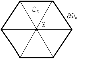
Refer to caption — Figure 3.1: Example of an interior reference patch $\widehat{\omega}_{\boldsymbol{z}}$

We recall that ${\mathcal{V}}$ is the set of all inner vertices, i.e., $\boldsymbol{z}\notin\partial\Gamma$ for all $\boldsymbol{z}\in{\mathcal{V}}$ . We define the patch size for a vertex $z\in{\mathcal{V}}$ as $h_{\boldsymbol{z}}:=\operatorname{diam}(\omega_{\boldsymbol{z}})$ and stress that $\gamma$ -shape regularity implies $h_{\boldsymbol{z}}\sim h|_{K}$ for all elements $T\subseteq\omega_{\boldsymbol{z}}$ .

Due to shape regularity, the number of elements meeting at a vertex is bounded. The following definition allows us to transform the vertex patches $\omega_{\boldsymbol{z}}$ to a finite number of reference configurations.

Definition 3.5 (reference patch).

Let $\omega_{\boldsymbol{z}}$ be an interior patch consisting of $n$ triangles. We may define a Lipschitz continuous bijective map $F_{\boldsymbol{z}}:\widehat{\omega}_{\boldsymbol{z}}\rightarrow\omega_{\boldsymbol{z}}$ , where $\widehat{\omega}_{\boldsymbol{z}}\subseteq\mathbb{R}^{2}$ is a regular polygon with $n$ edges, see Fig. 3.1. The map $F_{\boldsymbol{z}}$ is piecewise defined as a concatenation of affine maps from triangles comprising the regular polygon to the reference element $\widehat{K}$ with the element maps $F_{K}$ . We note that $F_{\boldsymbol{z}}(\partial\widehat{\omega}_{\boldsymbol{z}})=\partial\omega_{\boldsymbol{z}}$ .

The following lemma tells us how the hypersingular integral operator behaves under the patch transformation.

Lemma 3.6.

Let $u\in\widetilde{H}^{1/2}(\Gamma)$ with $\operatorname{supp}(u)\subseteq\overline{\omega_{\boldsymbol{z}}}$ . Define $\widehat{u}:=u\circ F_{\boldsymbol{z}}$ and the integral operator $\widehat{D}$ as $\widehat{D}\widehat{u}\,(x):=-\partial_{n_{x}}^{int}\int_{\widehat{\omega_{\boldsymbol{z}}}}{\partial_{n_{y}}^{int}G(x,y)\widehat{u}(y)\;ds(y)}\quad\text{for }x\in\widehat{\omega}_{\boldsymbol{z}}$ , where we treat $\widehat{\omega_{\boldsymbol{z}}}\subseteq\mathbb{R}^{2}$ as a screen embedded in $\mathbb{R}^{3}$ and $\partial_{n_{x}}$ is the derivative in direction of the vector $(0,0,1)$ . Then the hypersingular operator scales like

\left<Du,u\right>_{\omega_{\boldsymbol{z}}}\sim h_{\boldsymbol{z}}\left<\widehat{D}\widehat{u},\widehat{u}\right>_{\widehat{\omega}_{\boldsymbol{z}}},

where the implied constants depend only on $\Gamma$ and the $\gamma$ -shape regularity of $\mathcal{T}$ .

Proof.

We will prove this in three steps:

(i)

$\left<Du,u\right>_{\Gamma}\sim\left\|u\right\|_{\widetilde{H}^{1/2}(\omega_{\boldsymbol{z}})}^{2}$ ,
(ii)

$\left\|u\right\|_{\widetilde{H}^{1/2}(\omega_{\boldsymbol{z}})}^{2}\sim h_{\boldsymbol{z}}\left\|\widehat{u}\right\|_{\widetilde{H}^{1/2}(\widehat{\omega}_{\boldsymbol{z}})}^{2}$ ,
(iii)

$\left\|\widehat{u}\right\|_{\widetilde{H}^{1/2}(\widehat{\omega}_{\boldsymbol{z}})}^{2}\sim\left<\widehat{D}\widehat{u},\widehat{u}\right>_{\widehat{\omega}_{\boldsymbol{z}}}$ .

Proof of (i): It is well-known that $D$ is continuous and elliptic on $\widetilde{H}^{1/2}(\omega_{\boldsymbol{z}})$ . In our case, the ellipticity constants can be chosen independently of the patch $\omega_{\boldsymbol{z}}$ and instead only depend on $\Gamma$ . To do so we embed the spaces $\widetilde{H}^{1/2}(\omega_{\boldsymbol{z}})$ into finitely many larger spaces $\widetilde{H}^{1/2}(\mathcal{O}_{j})$ , where the sub-surfaces $\mathcal{O}_{j}$ are open and for each $\boldsymbol{z}$ there is ${\mathcal{O}}_{j}$ such that $\omega_{\boldsymbol{z}}\subseteq\mathcal{O}_{j}\subseteq\Gamma$ . (For the screen problem we may use the single sub-surface $\mathcal{O}:=\Gamma$ , for the case of closed surfaces we can, for example, use $\mathcal{O}_{j}:=\Gamma\setminus F_{j}$ , where $F_{j}$ is the $j$ -th face of the polyhedron $\Omega$ such that $\omega_{\boldsymbol{z}}\cap F_{j}=\emptyset$ ). It is important that these surfaces are open, since for closed surfaces $\Gamma$ we do not have full ellipticity of $D$ but only for $\widetilde{D}$ , and the stabilization term has a different scaling behavior. Since $u$ vanishes outside of $\omega_{\boldsymbol{z}}$ we can use the ellipticity on $\widetilde{H}^{1/2}(\mathcal{O}_{j})$ to see $\left<Du,u\right>_{\Gamma}\sim\left\|u\right\|_{\widetilde{H}^{1/2}(\mathcal{O}_{j})}^{2}$ . By Corollary 3.3 the norms on $\omega_{\boldsymbol{z}}$ and $\mathcal{O}_{j}$ are equivalent, which implies the statement (i).

Proof of (ii): The scalings of the $L^{2}$ -norm and $H^{1}$ -seminorm (we can use the seminorm, since we are working on $\widetilde{H}^{1/2}$ of an open surface) is well-known to be

\displaystyle\left\|u\right\|_{L^{2}(\omega_{\boldsymbol{z}})}

\displaystyle\sim h_{\boldsymbol{z}}\left\|\widehat{u}\right\|_{L^{2}(\widehat{\omega}_{\boldsymbol{z}})},\quad\left\|\nabla u\right\|_{L^{2}(\omega_{\boldsymbol{z}})}\sim\left\|\nabla\widehat{u}\right\|_{L^{2}(\widehat{\omega}_{\boldsymbol{z}})}.

The interpolation theorem (Proposition 2.1, (i)) then proves part (ii).

Proof of (iii): We again use ellipticity and continuity of $\widehat{D}$ . Since there are only finitely many reference patches, the constants can be chosen independently of the individual patches. ∎

4 Condition number of the $hp$ -Galerkin matrix

In this section we investigate the condition number of the unpreconditioned Galerkin matrix to motivate the need for good preconditioning. We will work on the reference triangle $\widehat{K}=\operatorname{conv}\left\{(0,0),(1,0),(0,1)\right\}$ and will need the following well-known inverse inequalities for polynomials on $\widehat{K}$ :

Proposition 4.1 (Inverse inequalities, [37, Theorem 4.76]).

Let $\widehat{K}$ denote the reference triangle and let ${\mathcal{E}}$ be one of its edges. There exists a constant $C$ such that for all $p\in\mathbb{N}$ and for all $v\in P^{p}(\widehat{K})$ the following estimates hold:

$\displaystyle\left\\|v\right\\|_{L^{\infty}(\widehat{K})}$	$\displaystyle\leq Cp^{2}\left\\|v\right\\|_{L^{2}(\widehat{K})},$	(4.1)
$\displaystyle\left\\|v\right\\|_{L^{\infty}(\widehat{K})}$	$\displaystyle\leq C\sqrt{\log(p+1)}\left\\|v\right\\|_{H^{1}(\widehat{K})},$	(4.2)
$\displaystyle\left\\|v\right\\|_{H^{1}(\widehat{K})}$	$\displaystyle\leq Cp^{2}\left\\|v\right\\|_{L^{2}(\widehat{K})},$	(4.3)
$\displaystyle\left\\|v\right\\|_{L^{2}({\mathcal{E}})}$	$\displaystyle\leq Cp\left\\|v\right\\|_{L^{2}(\widehat{K})}.$	(4.4)

∎

First we investigate the $L^{2}$ and $H^{1}$ conditioning of our basis on the reference triangle.

Lemma 4.2.

Let $u\in P^{p}(\widehat{K})$ and let $\alpha^{\mathcal{V}}_{j}$ , $\alpha_{j}^{\mathcal{E}_{m}}$ , $\alpha^{\mathcal{I}}_{(ij)}$ be the coefficients with respect to the basis in Definition 2.4, i.e., we decompose $u=u_{\mathcal{V}}+u_{\mathcal{E}_{1}}+u_{\mathcal{E}_{2}}+u_{\mathcal{E}_{3}}+u_{\mathcal{I}}$ with

\displaystyle u_{\mathcal{V}}

\displaystyle=\sum_{j=1}^{3}{\alpha^{\mathcal{V}}_{j}\varphi^{\mathcal{V}}_{j}},\quad u_{\mathcal{E}_{m}}=\sum_{j=0}^{p-2}{\alpha^{\mathcal{E}_{m}}_{j}\varphi^{\mathcal{E}_{m}}_{j}},\quad u_{\mathcal{I}}=\sum_{i+j\leq p-3}{\alpha^{\mathcal{I}}_{(ij)}\varphi^{\mathcal{I}}_{(ij)}}.

(4.5)

Then for a constant $C>0$ that does not depend on $u$ or $p$ :

\displaystyle\left\|u_{\mathcal{V}}\right\|_{L^{2}(\widehat{K})}^{2}

\displaystyle\leq C\sum_{j=1}^{3}{\left|\alpha^{\mathcal{V}}_{j}\right|^{2}},

\displaystyle\left\|u_{\mathcal{E}_{m}}\right\|_{L^{2}(\widehat{K})}^{2}

\displaystyle\leq C\sum_{j=0}^{p-2}{\left|\alpha^{\mathcal{E}_{m}}_{j}\right|^{2}},

\displaystyle\left\|u_{\mathcal{I}}\right\|_{L^{2}(\widehat{K})}^{2}

\displaystyle=\sum_{i+j\leq p-3}{\left|\alpha^{\mathcal{I}}_{(ij)}\right|^{2}}.

(4.6)

Combined this gives:

\displaystyle\left\|u\right\|_{L^{2}(\widehat{K})}^{2}

\displaystyle\leq C\Bigl(\sum_{j=1}^{3}{\left|\alpha^{\mathcal{V}}_{j}\right|^{2}}+\sum_{m=1}^{3}{\sum_{j=0}^{p-2}{\left|\alpha_{j}^{\mathcal{E}_{m}}\right|}^{2}}+\sum_{i+j\leq p-3}{\left|\alpha^{\mathcal{I}}_{(ij)}\right|^{2}}\Bigr).

(4.7)

Proof.

The estimate for $u_{\mathcal{V}}$ in (4.6) is clear. For the edge contributions in (4.6), we restrict ourselves to the edge $(0,0)-(1,0)$ , i.e., $m=1$ and drop the index $m$ in the notation. The other edges can be treated analogously.

	$\displaystyle\left\\|u_{\mathcal{E}}\right\\|_{L^{2}(\widehat{K})}^{2}$	$\displaystyle=\left\\|\sum_{j=0}^{p-2}{\alpha^{\mathcal{E}}_{j}\sqrt{\frac{2i+3}{2}}L^{\mathcal{S}}_{i+2}(\lambda_{1}-\lambda_{2},\lambda_{1}+\lambda_{2})}\right\\|^{2}_{L^{2}(\widehat{K})}$
		$\displaystyle=\sum_{i,j=0}^{p-2}{\alpha^{\mathcal{E}}_{j}\alpha^{\mathcal{E}}_{i}\int_{\widehat{K}}{\sqrt{\frac{2i+3}{2}}L^{\mathcal{S}}_{i+2}(\lambda_{1}-\lambda_{2},\lambda_{1}+\lambda_{2})}\sqrt{\frac{2j+3}{2}}L^{\mathcal{S}}_{j+2}(\lambda_{1}-\lambda_{2},\lambda_{1}+\lambda_{2})}dx$
		$\displaystyle=\frac{1}{4}\sum_{i,j=0}^{p-2}{\alpha^{\mathcal{E}}_{j}\alpha^{\mathcal{E}}_{i}\int_{-1}^{1}{\int_{-1}^{1}{\sqrt{\frac{2i+3}{2}}L_{i+2}(\xi)\sqrt{\frac{2j+3}{2}}L_{j+2}(\xi)\left(\frac{1-\eta}{2}\right)^{i+j+5}d\xi d\eta}}}.$

In the last step we transformed the reference triangle to $(-1,1)\times(-1,1)$ via the map ${(\xi,\eta)\mapsto(\frac{1}{4}(1+\xi)(1-\eta),\frac{1}{2}(1+\eta))}$ .

It is well-known (see [37, p. 65]) that the 1D-mass matrix M of the integrated Legendre polynomials is pentadiagonal, and the non-zero entries satisfy $\left|M_{(ij)}\right|\sim\frac{1}{(i+1)\,(j+1)}$ . It is easy to check that $\left|\int_{-1}^{1}{\left(\frac{1-\eta}{2}\right)^{i+j+5}d\eta}\right|\leq C(i+j+6)^{-1}$ . Together with a Cauchy-Schwarz estimate, we obtain:

\displaystyle\left\|u_{\mathcal{E}}\right\|_{L^{2}(\widehat{K})}^{2}

\displaystyle\lesssim\sum_{j=0}^{p-2}{\left|\alpha^{\mathcal{E}}_{j}\right|^{2}\frac{1}{(j+1)^{3}}}\lesssim\sum_{j=0}^{p-2}{\left|\alpha^{\mathcal{E}}_{j}\right|^{2}}.

The bubble basis functions are chosen $L^{2}$ -orthogonal. Thus, using our scaling of the bubble basis functions,

\displaystyle\left\|u_{\mathcal{I}}\right\|_{L^{2}(\widehat{K})}^{2}

\displaystyle=\sum_{i+j\leq p-3}{\left|\alpha^{\mathcal{I}}_{(ij)}\right|^{2}\left\|\varphi_{(ij)}\right\|_{L^{2}(\widehat{K})}^{2}}=\sum_{i+j\leq p-3}\left|\alpha^{\mathcal{I}}_{(ij)}\right|^{2}.

Finally, we split the function $u$ into vertex, edge and inner components, apply the triangle inequality and get

\displaystyle\left\|u\right\|_{L^{2}(\widehat{K})}^{2}

\displaystyle\leq 5\left\|u_{\mathcal{V}}\right\|^{2}_{L^{2}(\widehat{K})}+5\sum_{m=1}^{3}{\left\|u_{\mathcal{E}_{j}}\right\|_{L^{2}(\widehat{K})}^{2}}+5\left\|u_{\mathcal{I}}\right\|_{L^{2}(\widehat{K})}^{2},

which is (4.7). ∎

More interesting are the reverse estimates.

Lemma 4.3.

There is a constant $C>0$ independent of $p$ such for every $u\in P^{p}(\widehat{K})$ the coefficients of its representation in the basis of Definition 2.4 as in Lemma 4.2 satisfy:

	vertex parts:	$\displaystyle\qquad\sum_{j=1}^{3}{\left\|\alpha^{\mathcal{V}}_{j}\right\|^{2}}\leq Cp^{4}\left\\|u\right\\|_{L^{2}(\widehat{K})}^{2}\quad\text{ as well as }\quad\sum_{j=1}^{3}{\left\|\alpha^{\mathcal{V}}_{j}\right\|^{2}}\leq C\log(p+1)\left\\|u\right\\|_{H^{1}(\widehat{K})}^{2},$
	edge parts:	$\displaystyle\qquad\sum_{j=0}^{p-2}{\left\|\alpha^{\mathcal{E}_{m}}_{j}\right\|^{2}}\leq Cp^{6}\left\\|u\right\\|_{L^{2}(\widehat{K})}^{2}\quad\text{ and }\quad\sum_{j=0}^{p-2}{\left\|\alpha^{\mathcal{E}_{m}}_{j}\right\|^{2}}\leq Cp^{2}\left\\|u\right\\|_{H^{1}(\widehat{K})}^{2}.$

Moreover, if $u$ vanishes on $\partial\widehat{K}$ , then

\displaystyle\sum_{i+j\leq p-3}{\left|\alpha^{\mathcal{I}}_{(ij)}\right|^{2}}

\displaystyle=\left\|u\right\|_{L^{2}(\widehat{K})}^{2}.

(4.8)

Proof.

Since $\alpha^{\mathcal{V}}_{j}=u(\boldsymbol{z}_{j})$ where $\boldsymbol{z}_{j}$ denotes the $j-th$ vertex, we can use the $L^{\infty}$ -inverse estimates (4.1) and (4.2) to get estimates for the vertex part.

For the edge parts, we again only consider the bottom edge, ${\mathcal{E}}={\mathcal{E}}_{m}$ with $m=1$ . First we assume that $u$ vanishes in all vertices. If we consider the restriction of $u$ to the edge ${\mathcal{E}}$ we only have contributions by the edge basis, i.e., we can write

	$\displaystyle u\left(x,0\right)$	$\displaystyle=\sum_{i=0}^{p-2}{\alpha^{\mathcal{E}}_{i}\sqrt{\frac{2i+3}{2}}L_{i+2}(2x-1)},\quad x\in(0,1),$
	$\displaystyle\frac{\partial}{\partial x}u(x,0)$	$\displaystyle=\sum_{i=0}^{p-2}{\alpha^{\mathcal{E}}_{i}2\;\sqrt{\frac{2i+3}{2}}\ell_{i+1}(2x-1)},\quad x\in(0,1).$

The factor was chosen to get an $L^{2}$ -normalized basis, since we have $\left\|\ell_{i+1}\right\|_{L^{2}(-1,1)}^{2}=\frac{2}{2i+3}$ . The Legendre polynomials are orthogonal on $(-1,1)$ , and therefore simple calculations show

\displaystyle\left\|\frac{\partial u}{\partial x}\right\|_{L^{2}(\mathcal{E})}^{2}

\displaystyle=2\sum_{i=0}^{p-2}{\left|\alpha^{\mathcal{E}}_{i}\right|^{2}}.

If we consider a general $u\in P^{p}(\widehat{K})$ , we apply the previous estimate to $u_{2}:=u-I^{1}u$ where $I^{1}$ denotes the nodal interpolation operator to the linears. Then we get from the triangle inequality

\displaystyle\sum_{i=0}^{p-2}{\left|\alpha^{\mathcal{E}}_{i}\right|^{2}}

\displaystyle\leq 2\left\|\frac{\partial u}{\partial x}\right\|_{L^{2}(\mathcal{E})}^{2}+2\left\|\frac{\partial I^{1}u}{\partial x}\right\|_{L^{2}(\mathcal{E})}^{2}.

We apply the trace estimate (4.4) to the first part and the trace and norm equivalence for the second. We obtain:

\displaystyle\sum_{i=0}^{p-2}{\left|\alpha^{\mathcal{E}}_{i}\right|^{2}}

\displaystyle\lesssim p^{2}\left\|\frac{\partial u}{\partial x}\right\|_{L^{2}(\widehat{K})}^{2}+\left\|I^{1}u\right\|_{L^{2}(\widehat{K})}^{2}.

The $H^{1}$ estimate then follows from the $L^{\infty}$ estimate for the nodal interpolant (4.2). For the $L^{2}$ estimate we then simply use the inverse estimate (4.3).

For the equality (4.8) we note that if $u|_{\partial T}=0$ then $u=u_{\mathcal{I}}$ and thus we can use the equality in (4.6). ∎

Lemma 4.4.

There exist constants $c_{0}$ , $C_{0}$ , $c_{1}$ , $C_{1}>0$ independent of $p$ such that for every $u\in P^{p}(\widehat{K})$ its coefficients in the basis of Definition 2.4 as in Lemma 4.2 satisfy:

	$\displaystyle c_{0}\left\\|u\right\\|_{L^{2}(\widehat{K})}^{2}$	$\displaystyle\leq\sum_{j=1}^{3}{\left\|\alpha^{\mathcal{V}}_{j}\right\|^{2}}+\sum_{m=1}^{3}{\sum_{j=0}^{p-2}{\left\|\alpha_{j}^{\mathcal{E}_{m}}\right\|}^{2}}+\sum_{i+j\leq p-3}{\left\|\alpha^{\mathcal{I}}_{(ij)}\right\|^{2}}\leq C_{0}p^{6}\left\\|u\right\\|_{L^{2}(\widehat{K})}^{2},$		(4.9)
	$\displaystyle c_{1}p^{-4}\left\\|u\right\\|_{H^{1}(\widehat{K})}^{2}$	$\displaystyle\leq\sum_{j=1}^{3}{\left\|\alpha^{\mathcal{V}}_{j}\right\|^{2}}+\sum_{m=1}^{3}{\sum_{j=0}^{p-2}{\left\|\alpha_{j}^{\mathcal{E}_{m}}\right\|}^{2}}+\sum_{i+j\leq p-3}{\left\|\alpha^{\mathcal{I}}_{(ij)}\right\|^{2}}\leq C_{1}p^{2}\left\\|u\right\\|_{H^{1}(\widehat{K})}^{2}.$		(4.10)

Proof of (4.9): .

The lower bound was already shown in Lemma 4.2. For the upper bound we apply the preceding Lemma 4.3 to $u$ and see $\sum_{j=1}^{3}{\left|\alpha^{\mathcal{V}}_{j}\right|^{2}}\lesssim p^{4}\left\|u\right\|_{L^{2}(\widehat{K})}^{2}$ . For any edge ${\mathcal{E}}_{m}$ we get

\displaystyle\sum_{j=0}^{p-2}{\left|\alpha^{\mathcal{E}_{m}}_{j}\right|^{2}}

\displaystyle\lesssim p^{6}\left\|u\right\|_{L^{2}(\widehat{K})}^{2}.

Next we set $u_{2}:=u-u_{\mathcal{V}}-u_{\mathcal{E}}$ , where $u_{\mathcal{E}}$ is the sum of the edge contributions $u_{\mathcal{E}_{m}}$ . This function vanishes on the boundary of $\widehat{K}$ and we can apply Lemma 4.3 to get:

\displaystyle\sum_{i+j\leq p-3}{\left|\alpha^{\mathcal{I}}_{(ij)}\right|^{2}}

\displaystyle\lesssim\left\|u_{2}\right\|_{L^{2}(\widehat{K})}^{2}.

Since we can always estimate the $L^{2}$ norms by the $\ell^{2}$ norms of the coefficients (Lemma 4.2), we obtain

\displaystyle\left\|u_{2}\right\|_{L^{2}(\widehat{K})}^{2}

\displaystyle\leq 3\left\|u\right\|_{L^{2}(\widehat{K})}^{2}+3\left\|u_{\mathcal{V}}\right\|_{L^{2}(\widehat{K})}^{2}+3\left\|u_{\mathcal{E}}\right\|_{L^{2}(\widehat{K})}^{2}\lesssim\left\|u\right\|_{L^{2}(\widehat{K})}^{2}+p^{6}\left\|u\right\|_{L^{2}(\widehat{K})}^{2}+p^{4}\left\|u\right\|_{L^{2}(\widehat{K})}^{2}.

Proof of (4.10): The proof for the upper $H^{1}$ estimate works along the same lines, but using the sharper $H^{1}$ -estimates from Lemma 4.3 for the vertex and edge parts. For the lower estimate, we just make use of the inverse estimate (4.3) and the fact that the $L^{2}$ -norm is uniformly bounded by the coefficients, to conclude the proof. ∎

Figure 4.1: Numerical computation of the extremal eigenvalues of the mass matrices and the sum of mass and

H^{1}

-stiffness matrix

M+S

for the full system and different sub-blocks.

Example 4.5.

In Figure 4.1 we compare our theoretical bounds on the reference element from Lemma 4.4 with a numerical experiment that studies the maximal and minimal eigenvalues of the mass matrix $M$ and the stiffness matrix $S$ (corresponding to the bilinear form $(\nabla\cdot,\nabla\cdot)_{L^{2}(\widehat{K})}$ ). We focus on the full system and the subblocks that contributed the highest order in our theoretical investigations, i.e. the edge blocks $M_{\mathcal{E}}$ , $S_{\mathcal{E}}$ , and the block of inner basis functions $M_{\mathcal{I}}$ , $S_{\mathcal{I}}$ . We see that the estimates on the full condition numbers are not overly pessimistic: the numerics show a behavior of the minimal eigenvalue of $\mathcal{O}(p^{5.5})$ instead of $\mathcal{O}(p^{6})$ . If we focus solely on the edge contributions, we see that the bound we used for the lower eigenvalue is not sharp there. This can partly be explained by the fact that if no inner basis functions are present it is possible to improve the estimate (4.4) by a factor of $p$ . But since we also need to include the coupling of inner and edge basis functions this improvement in order is lost again when looking at the full systems.

The estimates on the reference triangle can now be transferred to the global space $\widetilde{S}^{p}(\mathcal{T})$ on quasiuniform meshes.

Theorem 4.6.

Let $\mathcal{T}$ be a quasiuniform triangulation with mesh size $h$ . With the polynomial basis on the reference triangle $\widehat{K}$ given by Definition 2.4, let $\{\varphi_{i}\,|\,i=1,\ldots,N\}$ be the basis of $\widetilde{S}^{p}(\mathcal{T})$ . Then there exist constants $c_{0}$ , $c_{1/2}$ , $c_{1}$ , $C_{0}$ , $C_{1/2}$ , $C_{1}>0$ that depend only on $\Gamma$ and the $\gamma$ -shape regularity of $\mathcal{T}$ , such that, for every $\mathfrak{u}\in\mathbb{R}^{N}$ and $u=\sum_{j=1}^{N}{\mathfrak{u}_{j}\varphi_{j}}\in\widetilde{S}^{p}(\mathcal{T})$ :

$\displaystyle c_{0}\frac{1}{h^{2}}\left\\|u\right\\|_{L^{2}(\Gamma)}^{2}$	$\displaystyle\leq\left\\|\mathfrak{u}\right\\|_{\ell^{2}}^{2}\leq C_{0}\frac{p^{6}}{h^{2}}\left\\|u\right\\|_{L^{2}(\Gamma)}^{2},$	(4.11)
$\displaystyle c_{1}p^{-4}\left\\|u\right\\|_{H^{1}(\Gamma)}^{2}$	$\displaystyle\leq\left\\|\mathfrak{u}\right\\|_{\ell^{2}}^{2}\leq C_{1}\left(p^{2}+h^{-2}\right)\left\\|u\right\\|_{H^{1}(\Gamma)}^{2},$	(4.12)
$\displaystyle c_{1/2}h^{-1}\,p^{-2}\left\\|u\right\\|_{\widetilde{H}^{1/2}(\Gamma)}^{2}$	$\displaystyle\leq\left\\|\mathfrak{u}\right\\|_{\ell^{2}}^{2}\leq C_{1/2}\left(\frac{p^{4}}{h}+h^{-2}\right)\left\\|u\right\\|_{\widetilde{H}^{1/2}(\Gamma)}^{2}.$	(4.13)

Proof.

The $L^{2}$ -estimate (4.11) can easily be shown by transforming to the reference element and applying (4.9).

To prove the other estimates (4.12), (4.13), we need the Scott-Zhang projection operator $J_{h}:L^{2}(\Gamma)\rightarrow\widetilde{S}^{1}(\mathcal{T})$ as modified in [3, Section 3.2]. It has the following important properties:

1.

$J_{h}$ is a bounded linear operator from $L^{2}(\Gamma)$ to $(\widetilde{S}^{1}(\mathcal{T}),\|\cdot\|_{L^{2}(\Gamma)})$ .
2.

For every $s\in[0,1]$ there holds $\left\|J_{h}v\right\|_{\widetilde{H}^{s}(\Gamma)}\leq C_{stab}(s)\left\|v\right\|_{\widetilde{H}^{s}(\Gamma)}$ $\forall v\in\widetilde{H}^{s}(\Gamma)$ .

For every $K\in\mathcal{T}$ let $\omega_{K}:=\bigcup\left\{K^{\prime}\in\mathcal{T}:K\cap K^{\prime}\neq\emptyset\right\}$ denote the element patch, i.e., the union of all elements that touch $K$ . Then, for all $v\in\widetilde{H}^{1}(\Gamma)$

	$\displaystyle\left\\|\left(1-J_{h}\right)v\right\\|_{L^{2}(K)}$	$\displaystyle\leq C_{sz}h_{K}\left\\|\nabla v\right\\|_{L^{2}(\omega_{K})},$		(4.14)
	$\displaystyle\left\\|\nabla\left(1-J_{h}\right)v\right\\|_{L^{2}(K)}$	$\displaystyle\leq C_{sz}\left\\|\nabla v\right\\|_{L^{2}(\omega_{K})}.$		(4.15)

The constant $C_{sz}$ depends only on the $\gamma$ -shape regularity of $\mathcal{T}$ , and $C_{stab}(s)$ additionally depends on $\Gamma$ and $s$ .

We will use the following notation: For a function $u\in\widetilde{S}^{p}(\mathcal{T})$ we will write $\mathfrak{u}\in\mathbb{R}^{N}$ for its representation in the basis $\{\varphi_{i}\,|\,i=1,\ldots,N\}$ . For an element $K\in\mathcal{T}$ we write $\mathfrak{u}|_{K}$ for the part of the coefficient vector that belongs to basis functions whose support intersects the interior of $K$ . In addition to the function $u\in\widetilde{S}^{p}(\mathcal{T})$ , we will employ the function $\tilde{u}:=u-J_{h}u$ . Its vector representation will be denoted $\tilde{\mathfrak{u}}\in\mathbb{R}^{N}$ . Finally, the vector representation of $J_{h}u$ (again $u\in\widetilde{S}^{p}(\mathcal{T})$ ) will be $\mathfrak{J}_{h}\mathfrak{u}\in\mathbb{R}^{N}$ .

1. step: We claim the following stability estimates:

$\displaystyle\left\\|\mathfrak{J}_{h}\mathfrak{u}\right\\|_{\ell^{2}}^{2}$	$\displaystyle\lesssim h^{-2}\,\left\\|J_{h}u\right\\|_{L^{2}(\Gamma)}^{2}\lesssim h^{-2}\left\\|u\right\\|_{L^{2}(\Gamma)}^{2}\lesssim\left\\|\mathfrak{u}\right\\|_{\ell^{2}}^{2},$	(4.16)
$\displaystyle\left\\|J_{h}u\right\\|_{\widetilde{H}^{1/2}(\Gamma)}^{2}$	$\displaystyle\lesssim\penalty\ h^{-1}\left\\|J_{h}u\right\\|_{L^{2}(\Gamma)}^{2},$	(4.17)
$\displaystyle\left\\|J_{h}u\right\\|_{\widetilde{H}^{1/2}(\Gamma)}^{2}$	$\displaystyle\lesssim h\left\\|\mathfrak{u}\right\\|_{\ell^{2}}^{2}.$	(4.18)

The inequalities (4.16) are just a simple scaling argument combined with the $L^{2}$ stability of the Scott-Zhang projection and (4.11). The inequality (4.17) follows from the inverse inequality (note that $J_{h}u$ has degree 1). Finally, (4.18) follows from combining (4.17) and (4.16).

2. step: Next, we investigate the function $\tilde{u}=u-J_{h}u$ . We claim the following estimates:

$\displaystyle\left\\|\tilde{u}\right\\|_{L^{2}(\Gamma)}^{2}$	$\displaystyle\lesssim h^{2}\left\\|\mathfrak{u}\right\\|_{\ell^{2}}^{2},$	(4.19)
$\displaystyle\left\\|\tilde{u}\right\\|_{H^{1}(\Gamma)}^{2}$	$\displaystyle\lesssim p^{4}\left\\|\mathfrak{u}\right\\|_{\ell^{2}}^{2},$	(4.20)
$\displaystyle\left\\|\tilde{u}\right\\|_{\widetilde{H}^{1/2}(\Gamma)}^{2}$	$\displaystyle\lesssim p^{2}\,h\left\\|\mathfrak{u}\right\\|_{\ell^{2}}^{2}.$	(4.21)

The estimate (4.19) is a simple consequence of (4.11) and the $L^{2}$ -stability of the Scott-Zhang operator $J_{h}$ . For the proof of (4.20), we combine a simple scaling argument with (4.10) and the stability estimate (4.16) to get

\displaystyle\left\|\tilde{u}\right\|_{H^{1}(\Gamma)}^{2}

\displaystyle\stackrel{{\scriptstyle\penalty\ \eqref{eqn:condition_estimates_tref_h1}}}{{\lesssim}}p^{4}\left\|\mathfrak{\tilde{u}}\right\|_{\ell^{2}}^{2}\stackrel{{\scriptstyle\penalty\ \eqref{est_jhu_coeff}}}{{\lesssim}}p^{4}\left\|\mathfrak{u}\right\|_{\ell^{2}}^{2}.

The bound (4.21) follows from the interpolation estimate of Proposition 2.1, (ii) and the estimates (4.19)–(4.20).

3. step: We assert:

$\displaystyle\left\\|\mathfrak{\tilde{u}}\right\\|_{\ell^{2}}^{2}$	$\displaystyle\lesssim\frac{p^{6}}{h^{2}}\left\\|u\right\\|_{L^{2}(\Gamma)}^{2},$	(4.22)
$\displaystyle\left\\|\mathfrak{\tilde{u}}\right\\|_{\ell^{2}}^{2}$	$\displaystyle\lesssim p^{2}\left\\|u\right\\|_{H^{1}(\Gamma)}^{2},$	(4.23)
$\displaystyle\left\\|\mathfrak{\tilde{u}}\right\\|_{\ell^{2}}^{2}$	$\displaystyle\lesssim\frac{p^{4}}{h}\left\\|u\right\\|_{\widetilde{H}^{1/2}(\Gamma)}^{2}.$	(4.24)

Again, (4.22) is a simple consequence of (4.11) and the $L^{2}$ -stability of the Scott-Zhang operator $J_{h}$ . For the bound (4.23) we calculate, using the equivalence (4.10) of the coefficient vector and the $H^{1}$ -norm on the reference triangle, together with the scaling properties of the $H^{1}$ - and $L^{2}$ -norms,

\displaystyle\left\|\mathfrak{\tilde{u}}\right\|_{\ell^{2}}^{2}

\displaystyle\leq\sum_{K\in\mathcal{T}}{\left\|\mathfrak{\tilde{u}}|_{K}\right\|_{\ell^{2}}^{2}}\stackrel{{\scriptstyle\penalty\ \eqref{eqn:condition_estimates_tref_h1},\text{scaling}}}{{\lesssim}}p^{2}\sum_{K\in\mathcal{T}}{\left(h^{-2}\left\|\tilde{u}\right\|_{L^{2}(K)}^{2}+\left|\tilde{u}\right|_{H^{1}(K)}^{2}\right)}.

By applying the local $L^{2}$ -interpolation estimate (4.14) and $H^{1}$ -stability (4.15) we get

\displaystyle\left\|\mathfrak{\tilde{u}}\right\|_{\ell^{2}}^{2}

\displaystyle\lesssim p^{2}\sum_{K\in\mathcal{T}}{\left\|u\right\|_{H^{1}(\omega_{K})}^{2}}\lesssim p^{2}\left\|u\right\|_{H^{1}(\Gamma)}^{2},

where in the last step we used the fact for shape regular meshes each element is contained in at most $M$ different patches, where $M$ depends solely on the shape regularity constant $\gamma$ .

We next prove (4.24). We apply Proposition 2.1, (i) to the map $\ell^{2}\to\widetilde{S}^{p}(\mathcal{T}):\;\mathfrak{u}\mapsto u$ , where the space $\widetilde{S}^{p}(\mathcal{T})$ is once equipped with the $L^{2}$ - and once with the $H^{1}$ -norm. By Proposition 3.4 interpolating between (4.19) and (4.20) yields $\left\|\mathfrak{\tilde{u}}\right\|_{\ell^{2}}^{2}\lesssim\left(p^{6}h^{-2}\,p^{2}\right)^{1/2}\left\|u\right\|^{2}_{\widetilde{H}^{1/2}(\Gamma)}\lesssim p^{4}h^{-1}\left\|u\right\|^{2}_{\widetilde{H}^{1/2}(\Gamma)}$ .

4. step: The above steps allow us to obtain the $H^{1}$ and $H^{1/2}$ estimates (4.12)—(4.13) of the theorem. We decompose $u=\tilde{u}+J_{h}u$ and correspondingly $\mathfrak{u}=\mathfrak{\tilde{u}}+\mathfrak{J}_{h}\mathfrak{u}$ . Then:

	$\displaystyle\left\\|\mathfrak{u}\right\\|_{\ell^{2}}^{2}\lesssim\left\\|\tilde{\mathfrak{u}}\right\\|_{\ell^{2}}^{2}+\left\\|\mathfrak{J}_{h}\mathfrak{u}\right\\|_{\ell^{2}}^{2},$	$\displaystyle\stackrel{{\scriptstyle(\ref{est_utilde_coeff_honehalf}),(\ref{est_jhu_coeff})}}{{\lesssim}}\frac{p^{4}}{h}\left\\|u\right\\|_{\widetilde{H}^{1/2}(\Gamma)}^{2}+\frac{1}{h^{2}}\left\\|u\right\\|_{L^{2}(\Gamma)}^{2}\lesssim\frac{p^{4}\,h+1}{h^{2}}\left\\|u\right\\|_{\widetilde{H}^{1/2}(\Gamma)}^{2},$
	$\displaystyle\left\\|u\right\\|_{\widetilde{H}^{1/2}(\Gamma)}^{2}\lesssim\left\\|\tilde{u}\right\\|_{\widetilde{H}^{1/2}(\Gamma)}^{2}+\left\\|J_{h}u\right\\|_{\widetilde{H}^{1/2}(\Gamma)}^{2}$	$\displaystyle\stackrel{{\scriptstyle(\ref{est_utilde_honehalf}),(\ref{est_jhu_honehalf})}}{{\lesssim}}p^{2}\,h\left\\|\mathfrak{u}\right\\|_{\ell^{2}}^{2}+h\left\\|\mathfrak{u}\right\\|_{\ell^{2}}^{2}\lesssim h\,p^{2}\left\\|\mathfrak{u}\right\\|_{\ell^{2}}^{2}.$

This shows (4.13). The $H^{1}$ estimate (4.12) follows along the same lines: An elementwise inverse estimate gives

\left\|u\right\|^{2}_{H^{1}(\Gamma)}\lesssim\frac{p^{4}}{h^{2}}\left\|u\right\|^{2}_{L^{2}(\Gamma)}\stackrel{{\scriptstyle\penalty\ \eqref{eqn:condition_numbers_l2}}}{{\lesssim}}p^{4}\|\mathfrak{u}\|^{2}_{\ell^{2}},

and the splitting $\mathfrak{u}=\tilde{\mathfrak{u}}+\mathfrak{J}_{h}\mathfrak{u}$ produces

\displaystyle\left\|\mathfrak{u}\right\|^{2}_{\ell^{2}}\lesssim\left\|\tilde{\mathfrak{u}}\right\|^{2}_{\ell^{2}}+\left\|\mathfrak{J}_{h}\mathfrak{u}\right\|^{2}_{\ell^{2}}{\stackrel{{\scriptstyle(\ref{est_utilde_coeff}),(\ref{est_jhu_coeff})}}{{\lesssim}}}\left(p^{2}+h^{-2}\right)\left\|u\right\|^{2}_{H^{1}(\Gamma)}.

∎

Corollary 4.7.

The spectral condition number of the unpreconditioned Galerkin matrix $\widetilde{D}^{p}_{h}$ can be bounded by

\displaystyle\kappa\left(\widetilde{D}^{p}_{h}\right)

\displaystyle\leq C\left(\frac{p^{2}}{h}+p^{6}\right)

with a constant $C>0$ that depends only on $\Gamma$ and the $\gamma$ -shape regularity of $\mathcal{T}$ .

Proof.

The bilinear form induced by the stabilized hypersingular operator is elliptic and continuous with respect to the $\widetilde{H}^{1/2}$ -norm. By applying the estimates (4.13) to the Rayleigh quotients we get the stated result. ∎

Remark 4.8.

In this section we did not consider the effect of diagonal scaling. The numerical results in Section 6 suggest that it improves the $p$ -dependence of the condition number significantly.

4.1 Quadrilateral meshes

The present paper focuses on meshes consisting of triangles. Nevertheless, in order to put the results of Section 4 in perspective, we include a short section on quadrilateral meshes. In [29], estimates similar to those of Lemma 4.4 have been derived for the case of the Babuška-Szabó basis on the reference square $\widehat{S}:=[-1,1]^{2}$ . We give a brief summary of the definitions and results.

Definition 4.9 (Babuška-Szabó basis).

(i)

On the reference interval $\widehat{I}:=[-1,1]$ , the basis functions are based on the integrated Legendre polynomials $L_{j}$ as defined in (2.10):

\displaystyle\varphi_{0}(x)

\displaystyle:=\frac{1}{2}(1-x),

\displaystyle\varphi_{1}(x)

\displaystyle:=\frac{1}{2}(1+x),

\displaystyle\varphi_{j}(x)

\displaystyle:=\frac{1}{\left\|\ell_{j-1}\right\|_{L^{2}(I)}}L_{j}(x)\quad\forall\,2\leq j\leq p.

(ii)

On the reference square $\widehat{S}$ , the basis of the “tensor product space” ${\mathcal{Q}}^{p}(\widehat{S})$ is given by the tensor product of the 1D basis functions: ${\{\varphi_{i}\otimes\varphi_{j}:0\leq i,j\leq p\}}$ .

For this basis, the following estimates hold:

Proposition 4.10 ([29, Theorem 1], [22, Theorem 4.1]).

Let $u\in\mathcal{Q}^{p}(\widehat{S})$ and let $\mathfrak{u}$ denote its coefficient vector with respect to the basis of Definition 4.9. Then the following estimates hold:

\displaystyle\left\|u\right\|_{L^{2}(\widehat{S})}^{2}

\displaystyle\lesssim\left\|\mathfrak{u}\right\|_{\ell^{2}}^{2}\lesssim p^{8}\left\|u\right\|_{L^{2}(\widehat{S})}^{2},

\displaystyle\quad\left\|u\right\|_{H^{1}(\widehat{S})}^{2}

\displaystyle\lesssim\left\|\mathfrak{u}\right\|_{\ell^{2}}^{2}\lesssim p^{4}\left\|u\right\|_{H^{1}(\widehat{S})}^{2}.

(4.25)

Remark 4.11.

In [29, Thm. 1], the estimates were only shown for the inner degrees of freedom, i.e., if $u|_{\partial\widehat{S}}=0$ . This restriction is removed in [22, Thm. 4.1].

Theorem 4.12.

Let $\mathcal{T}$ be a quasi-uniform, shape-regular affine mesh of quadrilaterals of size $h$ , and let $F_{K}:\widehat{S}\to K$ be the affine element map for $K\in\mathcal{T}$ . Let $u\in\widetilde{\mathcal{Q}}^{p}(\mathcal{T}):=\left\{u\in\widetilde{H}^{1/2}(\Gamma):u|_{K}\circ F_{K}\in\mathcal{Q}^{p}(\widehat{S})\;\;\forall K\in\mathcal{T}\right\}$ , and let $\mathfrak{u}$ denote its coefficient vector with respect to the basis of Definition 4.9. Then there exist constants $c_{0},c_{1},C_{0},C_{1}>0$ that depend only on $\Gamma$ and the $\gamma$ -shape regularity of $\mathcal{T}$ such that:

\displaystyle c_{0}h^{-2}\left\|u\right\|_{L^{2}(\Gamma)}^{2}

\displaystyle\leq\left\|\mathfrak{u}\right\|_{\ell^{2}}^{2}\leq C_{0}h^{-2}p^{8}\left\|u\right\|_{L^{2}(\Gamma)}^{2},

\displaystyle c_{1}\left\|u\right\|_{H^{1}(\Gamma)}^{2}

\displaystyle\leq\left\|\mathfrak{u}\right\|_{\ell^{2}}^{2}\leq C_{1}\left(p^{4}+h^{-2}\right)\left\|u\right\|_{H^{1}(\Gamma)}^{2}.

Proof.

The proof is completely analogous to that of Theorem 4.6. The only additional ingredient to Proposition 4.10 is an operator $J_{h}:L^{2}\to\widetilde{\mathcal{Q}}^{1}(\mathcal{T})$ that is bounded with respect to the $L^{2}$ and the $H^{1}$ -norm, reproduces homogeneous Dirichlet boundary conditions for the case of open surfaces, and has the approximation property $\displaystyle\left\|u-J_{h}u\right\|_{L^{2}(\Gamma)}\lesssim h\left|u\right|_{H^{1}(\Gamma)}.$ Such an operator was proposed, e.g., in [6]. The important estimates that need to be shown are (we again write $\widetilde{u}:=u-J_{h}u$ ):

	$\displaystyle\left\\|u\right\\|_{L^{2}(\Gamma)}^{2}$	$\displaystyle\lesssim h^{2}\left\\|\mathfrak{u}\right\\|_{\ell^{2}}^{2},$	$\displaystyle\left\\|u\right\\|_{H^{1}(\Gamma)}^{2}$	$\displaystyle\lesssim\left\\|\mathfrak{u}\right\\|_{\ell^{2}}^{2}$
	$\displaystyle\left\\|\mathfrak{u}\right\\|_{\ell^{2}}^{2}$	$\displaystyle\lesssim\frac{p^{8}}{h^{2}}\left\\|u\right\\|_{L^{2}(\Gamma)}^{2},$	$\displaystyle\left\\|\mathfrak{u}\right\\|_{\ell^{2}}^{2}$	$\displaystyle\lesssim\left\\|\mathfrak{\widetilde{u}}\right\\|_{\ell^{2}}^{2}+\left\\|\mathfrak{J_{h}u}\right\\|_{\ell^{2}}^{2}\lesssim{p^{4}}\left\\|u\right\\|_{H^{1}(\Gamma)}^{2}+h^{-2}\left\\|u\right\\|_{L^{2}(\Gamma)}^{2}.\qed$

Remark 4.13.

In the case of triangular meshes, Proposition 3.4 allowed us to infer $\widetilde{H}^{1/2}$ -condition number estimates in Corollary 4.7 by interpolating the discrete norm equivalences in $L^{2}$ and $H^{1}$ of Theorem 4.6. For meshes consisting of quadrilaterals, the result corresponding to Proposition 3.4 is currently not available in the literature. If we conjecture $\left[\left(\widetilde{\mathcal{Q}}^{p}(\mathcal{T}),\left\|\cdot\right\|_{L^{2}(\Gamma)}\right),\left(\widetilde{\mathcal{Q}}^{p}(\mathcal{T}),\left\|\cdot\right\|_{H^{1}(\Gamma)}\right)\right]_{1/2}=\left(\widetilde{\mathcal{Q}}^{p}(\mathcal{T}),\left\|\cdot\right\|_{\widetilde{H}^{1/2}(\Gamma)}\right)$ with equivalent norms, then Theorem 4.12 implies the following estimates:

	$\displaystyle h^{-1}\left\\|u\right\\|^{2}_{\widetilde{H}^{1/2}(\Gamma)}$	$\displaystyle\lesssim\left\\|\mathfrak{u}\right\\|^{2}_{\ell^{2}}\lesssim\left(h^{-1}p^{6}+h^{-2}\right)\left\\|u\right\\|_{\widetilde{H}^{1/2}(\Gamma)}^{2},$
	$\displaystyle\kappa\left(\widetilde{D}_{h}^{p}\right)$	$\displaystyle\lesssim h^{-1}+p^{6}.$

Remark 4.14.

[29] also analyzes the influence of diagonal preconditioning and shows that the condition number is improved by a factor of two in the exponents of $p$ . Although we did not make any theoretical investigations in this direction for the $H^{1/2}$ -case, our numerical experiments in Examples 6.2 and 6.3 for triangular meshes show that diagonal scaling improves the $p$ -dependence of the condition number from $\mathcal{O}(p^{5.5})$ to $\mathcal{O}(p^{2.5})$ .

Remark 4.15.

The Babuška-Szabó basis of Definition 4.9 is not the only one used on quadrilaterals or hexahedra. An important representative of other bases are the Lagrange interpolation polynomials associated with the Gauß-Lobatto points. This basis has the better $\mathcal{O}(p^{3})$ conditioning for the stiffness matrix and $\mathcal{O}(p^{2})$ for the mass matrix (see [32],[29, Sect. 6]). Using the same arguments as in the proof of Theorem 4.12, we get for the global $H^{1}$ -problem that the condition number behaves like $\mathcal{O}(p\,h^{-2}+p^{3})$ . If the conjecture of Remark 4.13 is valid, then we obtain for this basis for the hypersingular integral operator the condition number estimate $\kappa(\widetilde{D}_{h}^{p})\lesssim p^{5/2}+p^{-1/2}h^{-1}$ . (See the Appendix for details.)

5 $hp$ -preconditioning

5.1 Abstract additive Schwarz methods

Additive Schwarz preconditioners are based on decomposing a vector space $\mathds{V}$ into smaller subspaces $\mathds{V}_{i}$ , $i=0,\dots,J$ , on which a local problem is solved. We recall some of the basic definitions and important results. Details can be found in [42, chapter 2].

Let $a(\cdot,\cdot):\mathds{V}\times\mathds{V}\to\mathbb{R}$ be a symmetric, positive definite bilinear form on the finite dimensional vector space $\mathds{V}$ . For a given $f\in\mathds{V}^{\prime}$ consider the problem of finding $u\in\mathds{V}$ such that

\displaystyle a(u,v)

\displaystyle=f(v)\quad\forall v\in\mathds{V}.

We will write $A$ for the corresponding Galerkin matrix.

Let $\mathds{V}_{i}\subset\mathds{V},\;i=0,\dots,J$ , be finite dimensional vector spaces with corresponding prolongation operators $R_{i}^{T}:\mathds{V}_{i}\to\mathds{V}$ . We will commit a slight abuse of notation and also denote the matrix representation of the operator by $R^{T}_{i}$ , and $R_{i}$ is its transposed matrix. We also assume that $\mathds{V}$ permits a (in general not direct) decomposition into

\displaystyle\mathds{V}

\displaystyle=R_{0}^{T}\mathds{V}_{0}+\sum_{i=1}^{J}{R_{i}^{T}\mathds{V}_{i}}.

We assume that for each subspace $\mathds{V}_{i}$ a symmetric and positive definite bilinear form

\displaystyle\widetilde{a}_{i}(\cdot,\cdot):\mathds{V}_{i}\times\mathds{V}_{i}\to\mathbb{R},\quad i=0,\dots,J,

is given. We write $\widetilde{A}_{i}$ for the matrix representation of $\widetilde{a}_{i}(\cdot,\cdot)$ . Sometimes these bilinear forms are referred to as the “local solvers”; in the simplest case of “exact local solvers” they are just restrictions of $a(\cdot,\cdot)$ , i.e., $\widetilde{a}_{i}(u_{i},v_{i}):=a\left(R_{i}^{T}u_{i},R_{i}^{T}v_{i}\right)$ for all $u_{i},v_{i}\in\mathds{V}_{i}.$ Then, the corresponding additive Schwarz preconditioner is given by

\displaystyle B^{-1}:=\sum_{i=0}^{J}{R_{i}^{T}\widetilde{A}^{-1}_{i}R_{i}}.

The following proposition allows us to bound the condition number of the preconditioned system $B^{-1}A$ . The first part is often referred to as the Lemma of Lions (see [51, 27, 30]).

Proposition 5.1.

(a)

Assume that there exists a constant $C_{0}>0$ such that every $u\in\mathds{V}$ admits a decomposition $u=\sum_{i=0}^{J}{R_{i}^{T}\,u_{i}}$ with $u_{i}\in\mathds{V}_{i}$ such that

$\displaystyle\sum_{i=0}^{J}{\widetilde{a}_{i}(u_{i},u_{i})}\leq C_{0}\;a(u,u).$

Then, the minimal eigenvalue $\lambda_{min}(B^{-1}A)$ of $B^{-1}A$ satisfies $\lambda_{min}\left(B^{-1}A\right)\geq C_{0}^{-1}.$
(b)

Assume that there exists $C_{1}>0$ such that for every decomposition $u=\sum_{i=0}^{J}{R_{i}^{T}\,v_{i}}$ with $v_{i}\in\mathds{V}_{i}$ the following estimate holds:

$\displaystyle a(u,u)\leq C_{1}\sum_{i=0}^{J}{\widetilde{a}_{i}(v_{i},v_{i})}.$

Then, the maximal eigenvalue $\lambda_{max}(B^{-1}A)$ of $B^{-1}A$ satisfies $\lambda_{max}\left(B^{-1}A\right)\leq C_{1}$ .
(c)

These two estimates together give an estimate for the condition number of the preconditioned linear system:

$\displaystyle\kappa\left(B^{-1}A\right)$ $\displaystyle:=\frac{\lambda_{max}}{\lambda_{min}}\leq C_{0}C_{1}.$ ∎

5.2 An $hp$ -stable preconditioner

In order to define an additive Schwarz preconditioner, we decompose the boundary element space $\mathds{V}:=\widetilde{S}^{p}(\mathcal{T})$ into several overlapping subspaces. We define $\mathds{V}_{h}^{1}:=\widetilde{S}^{1}(\mathcal{T})$ as the space of globally continuous and piecewise linear functions on $\mathcal{T}$ that vanish on $\partial\Gamma$ and denote the corresponding canonical embedding operator by $R_{h}^{T}:\mathds{V}_{h}^{1}\to\mathds{V}$ . We also define for each vertex $\boldsymbol{z}\in{\mathcal{V}}$ the local space

\displaystyle\mathds{V}_{\boldsymbol{z}}^{p}:=\{u\in\widetilde{S}^{p}(\mathcal{T})|\operatorname{supp}(u)\subset\overline{\omega_{\boldsymbol{z}}}\}

and denote the canonical embedding operators by $R_{\boldsymbol{z}}^{T}:\mathds{V}_{\boldsymbol{z}}^{p}\to\mathds{V}$ . The space decomposition then reads

\displaystyle\mathds{V}=\mathds{V}_{h}^{1}+\sum_{\boldsymbol{z}\in{\mathcal{V}}}{\mathds{V}_{\boldsymbol{z}}^{p}}.

(5.1)

We will denote the restriction of the Galerkin matrix $\widetilde{D}_{h}^{p}$ to the subspaces $\mathds{V}_{h}^{1}$ and $\mathds{V}_{\boldsymbol{z}}^{p}$ as $\widetilde{D}_{h}^{1}$ and $\widetilde{D}^{p}_{h,\boldsymbol{z}}$ , respectively.

Lemma 5.2.

There exist constants $c_{1},c_{2}>0$ , which depend only on $\Gamma$ and the $\gamma$ -shape regularity of $\mathcal{T}$ , such that the following holds:

(a)

For every $u\in\widetilde{S}^{p}(\mathcal{T})$ there exists a decomposition $u=u_{1}+\sum_{\boldsymbol{z}\in{\mathcal{V}}}{u_{\boldsymbol{z}}}$ with $u_{1}\in\mathds{V}_{h}^{1}$ and $u_{\boldsymbol{z}}\in\mathds{V}^{p}_{\boldsymbol{z}}$ and

\displaystyle\left\|u_{1}\right\|_{\widetilde{H}^{1/2}(\Gamma)}^{2}+\sum_{\boldsymbol{z}\in{\mathcal{V}}}{\left\|u_{\boldsymbol{z}}\right\|_{\widetilde{H}^{1/2}(\Gamma)}^{2}}

\displaystyle\leq c_{1}\;\left\|u\right\|_{\widetilde{H}^{1/2}(\Gamma)}^{2}.

(b)

Any decomposition $u=v_{1}+\sum_{\boldsymbol{z}\in{\mathcal{V}}}{v_{\boldsymbol{z}}}$ with $v_{1}\in\mathds{V}^{1}_{h}$ and $v_{\boldsymbol{z}}\in\mathds{V}^{p}_{\boldsymbol{z}}$ satisfies

\displaystyle\left\|u\right\|_{\widetilde{H}^{1/2}(\Gamma)}^{2}

\displaystyle\leq c_{2}\left(\left\|v_{1}\right\|_{\widetilde{H}^{1/2}(\Gamma)}^{2}+\sum_{\boldsymbol{z}\in{\mathcal{V}}}{\left\|v_{\boldsymbol{z}}\right\|_{\widetilde{H}^{1/2}(\Gamma)}^{2}}\right).

Proof.

The first estimate is the assertion of Proposition 3.1, (iv). The second estimate can be shown by a so-called coloring argument, along the same lines as in [18, Lemma 2]. It is based on the following estimate (see [35, Lemma 4.1.49] or [46, Lemma 3.2]): Let $w_{j}$ , $j=1,\dots,n$ be functions in $\widetilde{H}^{s}(\Gamma)$ for $s\geq 0$ with pairwise disjoint support. Then it holds

\displaystyle\left\|\sum_{i=1}^{n}{w_{i}}\right\|_{\widetilde{H}^{s}(\Gamma)}^{2}

\displaystyle\leq C\sum_{i=1}^{n}{\left\|w_{i}\right\|^{2}_{\widetilde{H}^{s}(\Gamma)}},

(5.2)

where $C>0$ depends only on $\Gamma$ . By $\gamma$ -shape regularity, the number of elements in any vertex patch, and therefore also the number of vertices in a patch, is uniformly bounded by some constant $N_{c}$ which depends solely on $\gamma$ . Thus, we can divide the vertices into sets $J_{1},\dots,J_{N_{c}}$ such that $\bigcup_{i=1}^{N_{c}}{J_{i}}={\mathcal{V}}$ and $\left|\omega_{\boldsymbol{z}}\cap\omega_{\boldsymbol{z^{\prime}}}\right|=0$ for all $\boldsymbol{z},\boldsymbol{z^{\prime}}$ in the same index set $J_{i}$ . Repeated application of the triangle inequality together with (5.2) then gives:

	$\displaystyle\left\\|u\right\\|_{\widetilde{H}^{1/2}(\Gamma)}^{2}\leq 2\left\\|v_{1}\right\\|_{\widetilde{H}^{1/2}(\Gamma)}^{2}+2\left\\|\sum_{\boldsymbol{z}\in{\mathcal{V}}}{v_{\boldsymbol{z}}}\right\\|_{\widetilde{H}^{1/2}(\Gamma)}^{2}$	$\displaystyle\leq 2\left\\|v_{1}\right\\|_{\widetilde{H}^{1/2}(\Gamma)}^{2}+2N_{c}\sum_{i=1}^{N_{c}}{\left\\|\sum_{\boldsymbol{z}\in J_{i}}{v_{\boldsymbol{z}}}\right\\|_{\widetilde{H}^{1/2}(\Gamma)}^{2}}$
		$\displaystyle\leq 2\left\\|v_{1}\right\\|_{\widetilde{H}^{1/2}(\Gamma)}^{2}+2\,N_{c}\,C\sum_{\boldsymbol{z}\in{\mathcal{V}}}{\left\\|v_{\boldsymbol{z}}\right\\|_{\widetilde{H}^{1/2}(\Gamma)}^{2}}.\qed$

The previous lemma only made statements about the $\widetilde{H}^{1/2}(\Gamma)$ -norm.

Theorem 5.3.

Let $\mathcal{T}$ be a $\gamma$ -shape regular triangulation of $\Gamma$ . Then there is a constant $C>0$ that depends solely on $\Gamma$ and the $\gamma$ -shape regularity of ${\mathcal{T}}$ such that the following is true: The preconditioner

\displaystyle B^{-1}:=R^{T}_{h}\left(\widetilde{D}_{h}^{1}\right)^{-1}R_{h}\;+\;\sum_{\boldsymbol{z}\in{\mathcal{V}}}{R^{T}_{\boldsymbol{z}}\left(\widetilde{D}_{h,\boldsymbol{z}}^{p}\right)^{-1}}R_{\boldsymbol{z}},

which is implied by the space decomposition (5.1), leads to the spectral condition number estimate

\displaystyle\kappa(B^{-1}\widetilde{D}_{h}^{p})

\displaystyle\leq C.

Proof.

The bilinear form $\left<\widetilde{D}\cdot,\cdot\right>_{\Gamma}$ is equivalent to $\left\|{\cdot}\right\|^{2}_{\widetilde{H}^{1/2}(\Gamma)}$ . Hence, the combination of Lemma 5.2 and Proposition 5.1 give the boundedness of the condition number. ∎

5.3 Multilevel preconditioning on adaptive meshes

The preconditioner of Theorem 5.3 relies on the space decomposition (5.1). In this section, we discuss how the space $\widetilde{S}^{1}(\mathcal{T})$ of piecewise linear function can be further decomposed in a multilevel fashion. Our setting will be one where $\mathcal{T}$ is the finest mesh of a sequence $(\mathcal{T}_{\ell})_{\ell=0}^{L}$ of nested meshes that are generated by newest vertex bisection (NVB); see Figure 5.1 for a description. We point the reader to [40, 24] for a detailed discussion of NVB. A key feature of NVB is that it creates sequences of meshes that are uniformly shape regular. We mention in passing that further properties of NVB were instrumental in proving optimality of $h$ -adaptive algorithms in both FEM [8, 13] and BEM [11, 12, 15, 17]. Before discussing the details of the multilevel space decomposition, we stress that the preconditioner described in Section 5.2 is independent of the chosen refinement strategy (such as NVB) as long as it satisfies the assumptions in Section 5.2, whereas the condition number estimates for the local multilevel preconditioner discussed in the present Section 5.3 depend on the fact that the underlying refinement strategy is based on NVB.

Adaptive algorithms create sequences of meshes $(\mathcal{T}_{\ell})_{\ell=0}^{L}$ . Typically, the procedure starts with an initial triangulation $\mathcal{T}_{0}$ and the further members of the sequences are created inductively. That is, mesh $\mathcal{T}_{\ell}$ is obtained from $\mathcal{T}_{\ell-1}$ by refining some elements of $\mathcal{T}_{\ell-1}$ . In an adaptive environment, these elements are determined by a marking criterion (“marked elements”) and a mesh closure condition. Usually, the following assumptions on the mesh refinement are made:

1.

$\mathcal{T}_{\ell}$ is regular for all $\ell\in\mathbb{N}_{0}$ , i.e., there exist no hanging nodes;
2.

The meshes $\mathcal{T}_{0},\mathcal{T}_{1},\dots$ are uniformly $\gamma$ -shape-regular, i.e., with $|K|$ denoting the surface area of an element $K\in\mathcal{T}_{\ell}$ and $\mathrm{diam}(K)$ the Euclidean diameter, we have

$\displaystyle\sup_{\ell\in\mathbb{N}_{0}}\max_{K\in\mathcal{T}_{\ell}}\frac{\mathrm{diam}(K)^{2}}{|K|}\leq\gamma.$ (5.3)

We consider a sequence of triangulations $\mathcal{T}_{0},\dots,\mathcal{T}_{L}$ , which is created by iteratively applying NVB. The corresponding sets of vertices are denoted ${\mathcal{V}}_{0},\dots,{\mathcal{V}}_{L}$ . For a vertex ${\boldsymbol{z}}\in{\mathcal{V}}_{\ell}$ , the associated patch is denoted by $\omega_{\ell,{\boldsymbol{z}}}$ .

In the construction of the $p$ -preconditioner in Section 5.2 we only considered a single mesh $\mathcal{T}$ . For the remainder of the paper, the $p$ part will always be constructed with respect to the finest mesh $\mathcal{T}_{L}$ . For a simpler presentation we set $\mathcal{T}:=\mathcal{T}_{L}$ and ${\mathcal{V}}:={\mathcal{V}}_{L}$ .

5.3.1 A refined splitting for adaptive meshes

The space decomposition from (5.1) involves the global lowest-order space $\mathds{V}_{h}^{1}=\widetilde{S}^{1}(\mathcal{T}_{L})$ . Therefore, the computation of the corresponding additive Schwarz operator needs the inversion of a global problem, which is, in practice, very costly, and often even infeasible. To overcome this disadvantage, we consider a refined splitting of the space $\mathds{V}_{h}^{1}$ that relies on the hierarchy of the adaptively refined meshes $\mathcal{T}_{0},\dots,\mathcal{T}_{L}$ . The corresponding local multilevel preconditioner was introduced and analyzed in [14, 16]. See also [20, 47, 49, 48] for local multilevel preconditioners for (adaptive) FEM , [43, 19] for (uniform) BEM, and [2, 28, 44] for (restricted) approaches for adaptive BEM.

Set $\widetilde{\mathcal{V}}_{0}:={\mathcal{V}}_{0}$ and define the local subsets

\displaystyle\widetilde{\mathcal{V}}_{\ell}:={\mathcal{V}}_{\ell}\backslash{\mathcal{V}}_{\ell-1}\cup\{{\boldsymbol{z}}\in{\mathcal{V}}_{\ell-1}\,:\,\omega_{\ell,{\boldsymbol{z}}}\subsetneq\omega_{\ell-1,{\boldsymbol{z}}}\}\quad\text{for }\ell\geq 1

(5.4)

of newly created vertices plus some of their neighbors, see Figure 5.2 for a visualization. Based on these sets, we consider the space decomposition

\displaystyle\mathds{V}_{h}^{1}=\sum_{\ell=0}^{L}\sum_{{\boldsymbol{z}}\in\widetilde{\mathcal{V}}_{\ell}}\mathds{V}^{1}_{\ell,{\boldsymbol{z}}}\quad\text{with}\quad\mathds{V}^{1}_{\ell,{\boldsymbol{z}}}:=\mathrm{span}\{\varphi_{\ell,{\boldsymbol{z}}}\},

(5.5)

where $\varphi_{\ell,{\boldsymbol{z}}}\in\widetilde{S}^{1}(\mathcal{T}_{\ell})$ is the nodal hat function with $\varphi_{\ell,{\boldsymbol{z}}}({\boldsymbol{z}})=1$ and $\varphi_{\ell,{\boldsymbol{z}}}({\boldsymbol{z}}^{\prime})=0$ for all ${\boldsymbol{z}}^{\prime}\in{\mathcal{V}}_{\ell}\backslash\{{\boldsymbol{z}}\}$ . The basic idea of this splitting is that we do a diagonal scaling only in the regions where the meshes have been refined. We will use local exact solvers, i.e.,

\displaystyle\widetilde{a}_{\ell,{\boldsymbol{z}}}(u_{\ell,{\boldsymbol{z}}},v_{\ell,{\boldsymbol{z}}}):=\left<\widetilde{D}(R_{\ell,{\boldsymbol{z}}})^{T}u_{\ell,{\boldsymbol{z}}},(R_{\ell,{\boldsymbol{z}}})^{T}v_{\ell,{\boldsymbol{z}}}\right>_{\Gamma}\quad\text{for all }u_{\ell,{\boldsymbol{z}}},v_{\ell,{\boldsymbol{z}}}\in\mathds{V}^{1}_{\ell,{\boldsymbol{z}}},

where $(R_{\ell,{\boldsymbol{z}}})^{T}:\mathds{V}^{1}_{\ell,{\boldsymbol{z}}}\to\mathds{V}_{h}^{1}$ denotes the canonical embedding operator. Let $\widetilde{D}_{h}^{1}$ denote the Galerkin matrix of $\widetilde{D}$ with respect to the basis $(\varphi_{L,{\boldsymbol{z}}})_{{\boldsymbol{z}}\in{\mathcal{V}}_{L}}$ of $\mathds{V}_{h}^{1}$ and define $\widetilde{D}_{\ell,{\boldsymbol{z}}}^{1}:=\widetilde{a}_{\ell,{\boldsymbol{z}}}(\varphi_{\ell,{\boldsymbol{z}}},\varphi_{\ell,{\boldsymbol{z}}})$ . Then, the local multilevel diagonal (LMLD) preconditioner associated to the splitting (5.5) reads

\displaystyle(B_{h}^{1})^{-1}:=\sum_{\ell=0}^{L}\sum_{{\boldsymbol{z}}\in\widetilde{\mathcal{V}}_{\ell}}(R_{\ell,{\boldsymbol{z}}})^{T}\left(\widetilde{D}_{\ell,{\boldsymbol{z}}}^{1}\right)^{-1}R_{\ell,{\boldsymbol{z}}}.

(5.6)

We stress that this preconditioner corresponds to a diagonal scaling with respect to the local subset of vertices $\widetilde{\mathcal{V}}_{\ell}$ on each level $\ell=0,\dots,L$ . Further details and the proof of the following result are found in [14, 16].

Proposition 5.4.

The splitting (5.5) together with $\widetilde{a}_{\ell,{\boldsymbol{z}}}(\cdot,\cdot)$ and the operators $R_{\ell,\boldsymbol{z}}^{T}$ satisfies the requirements of Proposition 5.1 with constants depending only on $\Gamma$ and the initial triangulation $\mathcal{T}_{0}$ . For the additive Schwarz operator $P_{h}^{1}:=(B_{h}^{1})^{-1}\widetilde{D}_{h}^{1}$ , there holds in particular

\displaystyle c\left<\widetilde{D}u_{h},u_{h}\right>_{\Gamma}\leq\left<\widetilde{D}P_{h}^{1}u_{h},u_{h}\right>_{\Gamma}\leq C\left<\widetilde{D}u_{h},u_{h}\right>_{\Gamma}\quad\text{for all }u_{h}\in\mathds{V}_{h}^{1}.

(5.7)

The constants $c$ , $C>0$ depend only on $\Gamma$ , the initial triangulation $\mathcal{T}_{0}$ , and the use of NVB for refinement, i.e., $\mathcal{T}_{\ell+1}=\operatorname{refine}(\mathcal{T}_{\ell},\mathcal{M}_{\ell})$ with arbitrary set $\mathcal{M}_{\ell}\subseteq\mathcal{T}_{\ell}$ of marked elements. ∎

We replace the space $\mathds{V}_{h}^{1}$ in (5.1) by the refined splitting (5.5) and end up with the space decomposition

\displaystyle\mathds{V}=\sum_{\ell=0}^{L}\sum_{{\boldsymbol{z}}\in\widetilde{{\mathcal{V}}}_{\ell}}\mathds{V}^{1}_{\ell,{\boldsymbol{z}}}+\sum_{{\boldsymbol{z}}\in{\mathcal{V}}_{L}}\mathds{V}_{L,\boldsymbol{z}}^{p}.

(5.8)

The following Lemma 5.5 shows that the preconditioner resulting from the decomposition (5.8) is $hp$ -stable. The result formalizes the observation that the combination of stable subspace decompositions leads again to a stable subspace decomposition. It is a simple consequence of the well-known theory for additive Schwarz methods; see Section 5.1. Therefore, details are left to the reader.

Lemma 5.5.

Let $\mathds{V}$ be a finite dimensional vector space, and let $\mathds{V}_{j}$ , $R_{\mathds{V},j}^{T}$ , and $\widetilde{a}_{\mathds{V},j}(\cdot,\cdot)$ for $j=0,\dots,J$ be a decomposition of $\mathds{V}$ in the sense of Section 5.1 that satisfies the assumptions of Proposition 5.1 with constants $C_{0,\mathds{V}}$ and $C_{1,\mathds{V}}$ . Consider an additional decomposition $\mathds{W}_{\ell}$ , $R_{\mathds{W},{\ell}}^{T}$ and $\widetilde{a}_{\mathds{W},\ell}(\cdot,\cdot)$ with $\ell=0,\dots,L$ of $\mathds{V}_{0}$ that also satisfies the requirements of Proposition 5.1 for the bilinear form $\widetilde{a}_{\mathds{V},0}(\cdot,\cdot)$ with constants $C_{0,\mathds{W}}$ and $C_{1,\mathds{W}}$ . Define a new additive Schwarz preconditioner as:

\displaystyle\widetilde{B}^{-1}:=R_{\mathds{V},0}^{T}\left(\sum_{\ell=0}^{L}{R_{\mathds{W},\ell}^{T}\widetilde{A}_{\mathds{W},\ell}^{-1}R_{\mathds{W},\ell}}\;\right)R_{\mathds{V},0}\;+\;\sum_{j=1}^{J}{R_{\mathds{V},j}^{T}\widetilde{A}_{\mathds{V},j}^{-1}R_{\mathds{V},j}}.

This new preconditioner satisfies the assumptions of Proposition 5.1 with $C_{0}=\max\left(1,C_{0,\mathds{W}}\right)C_{0,\mathds{V}}$ and $C_{1}=\max\left(1,C_{1,\mathds{W}}\right)C_{1,\mathds{V}}$ . ∎

Theorem 5.6.

Assume that $\mathcal{T}$ is generated from a regular and shape-regular initial triangulation $\mathcal{T}_{0}$ by successive application of NVB. Based on the space decomposition (5.8) define the preconditioner

\displaystyle B_{2}^{-1}:=R_{h}^{T}(B_{h}^{1})^{-1}R_{h}\;+\;\sum_{\boldsymbol{z}\in{\mathcal{V}}_{L}}{R^{T}_{\boldsymbol{z}}\left(\widetilde{D}_{h,\boldsymbol{z}}^{p}\right)^{-1}}R_{\boldsymbol{z}}.

Then, for constants $c$ , $C>0$ that depend only on $\Gamma$ , $\mathcal{T}_{0}$ , and the use of NVB refinement, the extremal eigenvalues of $B_{2}^{-1}\widetilde{D}_{h}^{p}$ satisfy

\displaystyle c\leq\lambda_{\mathrm{min}}(B_{2}^{-1}\widetilde{D}_{h}^{p})\leq\lambda_{\mathrm{max}}(B_{2}^{-1}\widetilde{D}_{h}^{p})\leq C.

In particular, the condition number $\kappa(B_{2}^{-1}\widetilde{D}_{h}^{p})$ is bounded independently of $h$ and $p$ .

Proof.

The proof follows from Lemma 5.2, Proposition 5.4, and Lemma 5.5. ∎

5.4 Spectrally equivalent local solvers

For each vertex patch, we need to store the dense matrix $\left(\widetilde{D}^{p}_{h,\boldsymbol{z}}\right)^{-1}$ . For higher polynomial orders, storing these blocks is a significant part of the memory consumption of the preconditioner. To reduce these costs, we can make use of the fact that the abstract additive Schwarz theory allows us to replace the local bilinear forms $a(R^{T}_{i}u_{i},R^{T}_{i}v_{i})$ with spectrally equivalent forms, as long as they satisfy the conditions stated in Proposition 5.1. This is for example the case, if the decomposition is stable for the exact local solvers and if there exist constants $c_{1}$ , $c_{2}>0$ such that

\displaystyle c_{1}\,\widetilde{a}_{i}(u_{i},u_{i})

\displaystyle\leq a(R^{T}_{i}u_{i},R^{T}_{i}u_{i})\leq c_{2}\widetilde{a}_{i}(u_{i},u_{i})\quad\forall u_{i}\in\mathds{V}_{i}.

The new preconditioner will be based on a finite number of reference patches, for which the Galerkin matrix has to be inverted.

First we prove the simple fact that we can drop the stabilization term from (2.4) when assembling the local bilinear forms:

Lemma 5.7.

There exists a constant $c_{1}>0$ that depends only on $\Gamma$ and the $\gamma$ -shape regularity of $\mathcal{T}$ such that for any vertex patch $\omega_{\boldsymbol{z}}$ the following estimates hold:

\displaystyle\left<Du,u\right>_{\Gamma}

\displaystyle\leq\left<\widetilde{D}u,u\right>_{\Gamma}\leq c_{1}\left<Du,u\right>_{\Gamma}\qquad\forall u\in\mathds{V}^{p}_{\boldsymbol{z}}.

Proof.

The first estimate is trivial, as $\widetilde{D}$ only adds an additional non-negative term. For the second inequality, we note that the functions in $\mathds{V}^{p}_{\boldsymbol{z}}$ all vanish outside of $\omega_{\boldsymbol{z}}$ and therefore $\mathds{V}^{p}_{\boldsymbol{z}}\cap\operatorname{ker}(D)=\{0\}$ . We transform to the reference patch, use the fact that $\widehat{D}$ is elliptic on $\widetilde{H}^{1/2}(\widehat{\omega}_{\boldsymbol{z}})$ , and transform back by applying Lemma 3.6:

\displaystyle\left\|u\right\|_{L^{2}(\omega_{\boldsymbol{z}})}^{2}

\displaystyle\lesssim h_{\boldsymbol{z}}^{2}\left\|\widehat{u}\right\|_{L^{2}\left(\widehat{\omega}_{\boldsymbol{z}}\right)}^{2}\lesssim h_{\boldsymbol{z}}^{2}\left\|\widehat{u}\right\|_{\widetilde{H}^{1/2}(\widehat{\omega}_{\boldsymbol{z}})}^{2}\lesssim h_{\boldsymbol{z}}^{2}\left<\widehat{D}\widehat{u},\widehat{u}\right>_{\widehat{\omega}_{\boldsymbol{z}}}\lesssim h_{\boldsymbol{z}}\,\left<Du,u\right>_{\omega_{\boldsymbol{z}}}.

Thus, we can simply estimate the stabilization:

\displaystyle\alpha^{2}\left<u,\mathds{1}\right>_{\omega_{\boldsymbol{z}}}^{2}

\displaystyle\leq\alpha^{2}\left\|u\right\|^{2}_{L^{2}(\omega_{\boldsymbol{z}})}\left\|\mathds{1}\right\|^{2}_{L^{2}(\omega_{\boldsymbol{z}})}\leq C\alpha^{2}\left\|\mathds{1}\right\|_{L^{2}(\omega_{\boldsymbol{z}})}^{2}\,h_{\boldsymbol{z}}\;\left<Du,u\right>_{\Gamma}.

This gives the full estimate with the constant $c_{1}:=\max\left(1,\alpha^{2}\left\|\mathds{1}\right\|_{L^{2}(\omega_{\boldsymbol{z}})}^{2}\,Ch_{\boldsymbol{z}}\right)\leq\max\left(1,C\alpha^{2}h_{\boldsymbol{z}}^{3}\right)$ . ∎

Remark 5.8.

The proof of the previous lemma shows that this modification does not significantly affect the stability of the preconditioner and its effect will even vanish with $h$ -refinement.

We are now able to define the new local bilinear forms as:

Definition 5.9.

Take $\boldsymbol{z}\in{\mathcal{V}}$ and let $F_{\boldsymbol{z}}:\widehat{\omega}_{\boldsymbol{z}}\to\omega_{\boldsymbol{z}}$ be the pullback mapping to the reference patch as in Definition 3.5. Set

\displaystyle\widetilde{a}_{\boldsymbol{z}}(u,v):=h_{\boldsymbol{z}}\left<\widehat{D}\left(\;u\circ F_{\boldsymbol{z}}\right),v\circ F_{\boldsymbol{z}}\right>_{\widehat{\omega}_{\boldsymbol{z}}}\qquad\forall u,v\in\mathds{V}^{p}_{\boldsymbol{z}}.

(see Lemma 3.6 for the definition of $\widehat{D}$ ). We denote the Galerkin matrix corresponding the bilinear form $\widetilde{a}_{\boldsymbol{z}}$ on the reference patch by $\widehat{D}_{h,\operatorname{ref}(\boldsymbol{z})}^{p}$ .

The above definition only needs to evaluate $\left<\widehat{D}\widehat{u},\widehat{v}\right>_{\Gamma}$ on the reference patch. Since the reference patch depends only on the number of elements belonging to the patch, the number of blocks that need to be stored, depends only on the shape regularity and is independent of the number of vertices in the triangulation $\mathcal{T}$ .

Theorem 5.10.

Assume that $\mathcal{T}$ is generated from a regular and shape-regular initial triangulation $\mathcal{T}_{0}$ by successive application of NVB. The preconditioner using the local solvers from Definition 5.9 is optimal, i.e., for

\displaystyle B_{3}^{-1}:=R_{h}^{T}(B_{h}^{1})^{-1}R_{h}\;+\;\sum_{\boldsymbol{z}\in{\mathcal{V}}_{L}}{h_{\boldsymbol{z}}^{-1}R^{T}_{\boldsymbol{z}}\left(\widehat{D}_{h,\operatorname{ref}(\boldsymbol{z})}^{p}\right)^{-1}}R_{\boldsymbol{z}},

the condition number of the preconditioned system satisfies

\displaystyle\kappa(B_{3}^{-1}\tilde{D}_{h}^{p})\leq C,

where $C>0$ depends only on $\Gamma$ , $\mathcal{T}_{0}$ and the use of NVB refinement. It is in particular independent of $h$ and $p$ .

Proof.

The scaling properties of $\left<Du,u\right>_{\Gamma}$ were stated in Lemma 3.6. Therefore, we can conclude the argument by using the standard additive Schwarz theory. ∎

5.4.1 Numerical realization

Figure 5.3: The mapping to the reference patch described as a combination of element maps.

When implementing the preconditioner as defined above, it is important to note that for a basis function $\varphi_{i}$ on $\omega_{\boldsymbol{z}}$ the transformed function $\varphi_{i}\circ F_{\boldsymbol{z}}^{-1}$ does not necessarily correspond to the $i$ -th basis function on $\widehat{\omega}_{\boldsymbol{z}}$ . Depending on the chosen basis we may run into orientation difficulties. This can be resolved in the following way:

Let $\boldsymbol{z}\in{\mathcal{V}}$ be fixed. Choose a numbering for the vertices $\boldsymbol{z}_{i}$ and elements $K_{i}$ of $\omega_{\boldsymbol{z}}$ such that adjacent elements have adjacent numbers (for example, enumerate clockwise or counter-clockwise). We also choose a similar enumeration on the reference patch and denote it as $\widehat{\boldsymbol{z}}_{i}$ and $\widehat{K}_{i}$ . The enumeration is such that the reference map $F_{\boldsymbol{z}}$ maps $\boldsymbol{z}_{i}$ to $\widehat{\boldsymbol{z}_{i}}$ and $K_{i}$ to $\widehat{K}_{i}$ . Let $N_{\boldsymbol{z}}$ be the number of vertices in the patch.

For elements $K\subset\omega_{\boldsymbol{z}}$ and $K^{\prime}\subset\widehat{\omega}_{\boldsymbol{z}}$ , the bases on $\omega_{\boldsymbol{z}}$ and on $\widehat{\omega}_{\boldsymbol{z}}$ are locally defined by the pullback of polynomials on the reference triangle $\widehat{K}$ . We denote the element maps as $F_{K}:\widehat{K}\to K$ and $F_{K}^{\prime}:\widehat{K}\to K^{\prime}$ , respectively. The basis functions are then given as $\varphi_{j}:=\widehat{\varphi}_{j}\circ F_{K}$ on $\omega_{\boldsymbol{z}}$ and $\psi_{j}:=\widehat{\psi}_{j}\circ F_{K^{\prime}}$ on $\widehat{\omega}_{\boldsymbol{z}}$ . Corresponding local element maps do not necessarily map the same vertices of the reference element $\widehat{K}$ to vertices with the same numbers in the local ordering. Hence, we need to introduce another map $Q:\widehat{K}\to\widehat{K}$ that represents a vertex permutation. Then, we can write the patch-pullback restricted to $K^{\prime}$ as $F_{\boldsymbol{z}}|_{K^{\prime}}=F_{K}\circ Q\circ F_{K^{\prime}}^{-1}$ (see Figure 5.3). We observe:

i)

For the hat function the mapping is trivial: $\varphi_{\boldsymbol{z}}\circ F_{\boldsymbol{z}}=\psi_{\widehat{\boldsymbol{z}}}$ .
ii)

For the edge basis, permuting the vertices on the reference element only changes the sign of the corresponding edge functions. Thus, we have $\varphi^{{\mathcal{E}}_{m}}_{j}\circ F_{\boldsymbol{z}}=(-1)^{j}\psi^{{\mathcal{E}}_{m}}_{j}$ , if the orientation of the edge in the global triangulation does not match the orientation of the reference patch.
iii)

The inner basis functions transformation under $Q$ is not so simple. Since the basis functions all have support on a single element we can restrict our consideration to this element and assemble the necessary basis transformations for all 5 permutations of vertices on the reference triangle without losing the memory advantage of using the reference patch.

Remark 5.11.

One could also exploit the symmetry (up to a sign change) of the permutation of $\lambda_{1}$ and $\lambda_{2}$ in the definition of the inner basis functions to reduce the number of basis transformation matrices needed from 5 to 2.

6 Numerical results

The following numerical experiments confirm that the proposed preconditioners (Theorem 5.3, Theorem 5.6, and Theorem 5.10) do indeed yield a system with a condition number that is bounded uniformly in $h$ and $p$ , whereas the condition number of the unpreconditioned system grows in $p$ with a rate slightly smaller than predicted in Corollary 4.7: We observe numerically $\kappa\sim\mathcal{O}(p^{5.5})$ . Diagonal preconditioning appears to reduce the condition number to $\mathcal{O}(p^{2.5})$ . All of the following experiments were performed using the BEM++ software library ([38]; www.bempp.org) with the AHMED software library for $\mathcal{H}$ -matrix compression, [4], [5]. We used the polynomial basis described in Section 2.2.

Example 6.1 (unpreconditioned $p$ -dependence).

We consider a quadratic screen in $\mathbb{R}^{3}$ (see Figure 6.1, right). We study the $p$ -dependence of the unpreconditioned system on different uniformly refined meshes. In accordance with the estimates of Corollary 4.7, Figure 6.2 shows that one has, depending on the mesh size $h$ , a preasymptotic phase in which the $\mathcal{O}(h^{-1}p^{2})$ term dominates, and an $h$ -independent asymptotic $\mathcal{O}(p^{5.5})$ behavior. The latter is slightly better than the prediction of $\mathcal{O}(p^{6})$ of Corollary 4.7.

Figure 6.2: Comparison of the condition number of

\widetilde{D}^{p}_{h}

for the screen problem on different uniform meshes (Example 6.1)

Example 6.2 (Fichera’s cube).

We compare the preconditioner that uses the local multilevel preconditioner for the $h$ -part and the inexact local solvers based on the reference patches to the unpreconditioned system and to simple diagonal scaling. We consider the problem on a closed surface, namely, the surface of the Fichera cube with side length $2$ , and employ a stabilization parameter $\alpha=0.2$ . To generate the adaptive meshes, we used NVB, where in each step, the set of marked elements originated from a lowest order adaptive algorithm with a ZZ-type error estimator (as described in [3]). The left part of Figure 6.1 shows an example of one of the meshes used.

Figure 6.3 confirms that the condition number of the preconditioned system does not depend on the polynomial degree of the discretization. Figure 6.4 confirms the robustness of the preconditioner with respect to the adaptive refinement level. The unpreconditioned and the diagonally preconditioned system do not show a bad behavior with respect to $h$ , probably due to the already large condition number for $p>1$ .

Figure 6.4: Fichera cube, adaptive

h

-refinement for

p=3

(Example 6.2).

Example 6.3 (screen problem).

We consider the screen problem in $\mathbb{R}^{3}$ with a quadratic screen of side length 1 (see Figure 6.1, right), which represents the case $\Gamma\neq\partial\Omega$ and $\alpha=0$ in (2.3), and perform the same experiments as we did for Fichera’s cube in Example 6.2. In Figure 6.5 we again observe that the condition number is independent of the polynomial degree. Figures 6.6–6.9 demonstrate the independence of the mesh size $h$ .

Figure 6.5: Screen problem, condition numbers for uniform mesh with

45

elements (Example 6.3).

Figure 6.6: Screen problem, uniform

h

-refinement for

p=4

(Example 6.3).

Example 6.4 (inexact local solvers).

We compare the different preconditioners proposed in this paper. While the numerical experiments all show that the preconditioner is indeed robust in $h$ and $p$ , the constant differs if we use the different simplifications described in the Sections 5.3 and 5.4 to the preconditioner. In Figures 6.10 and 6.11, we can observe the different constants for the geometry given by Fichera’s cube of Example 6.2.

Figure 6.10: Comparison of the different proposed preconditioners for a fixed uniform mesh with

70

elements on the Fichera cube (Example 6.4).

Figure 6.11: Comparison of the different proposed preconditioners for adaptive mesh refinement on the Fichera cube with

p=2

Example 6.5 (inexact local solvers).

We continue with the geometry of Example 6.4, i.e., Fichera’s cube. We motivated Section 5.4 by stating the large memory requirement of the preconditioner when storing the dense local block inverses. It can be seen in Table 6.1 that the reference patch based preconditioner resolves this issue: we present the memory requirements for the various approaches when excluding the memory requirement for the treatment of the lowest order space $\mathds{V}_{h}^{1}$ . For comparison, we included the storage requirements for the full matrix $\widetilde{D}_{h}^{p}$ and the $\mathcal{H}$ -matrix approximation with accuracy $10^{-8}$ which is denoted as $D^{p,\mathcal{H}}_{h}$ . While we still get linear growth in the number of elements, due to some bookkeeping requirements, such as element orientation etc., which could theoretically also be avoided, we observe a much reduced storage cost. For $p=3$ and $55,298$ degrees of freedom, the memory requirement is less than $2.5\%$ of the full block storage. For $p=4$ and $393,218$ degrees of freedom the memory requirement is just $0.6\%$ and for higher polynomial orders, this ratio would become even smaller. Comparing only the number of blocks that need to be stored, we see that in this particular geometry we only need to store the inverse for $6$ reference blocks.

$p$	$N_{dof}$	$\operatorname{mem}\left(\widetilde{D}^{p}_{h}\right)/{N_{dof}}$	$\operatorname{mem}\left(\widetilde{D}^{p,\mathcal{H}}_{h}\right)/N_{dof}$	$\operatorname{mem}\left(B^{-1}\right)/N_{dof}$	$\operatorname{mem}\left(B_{3}^{-1}\right)/N_{dof}$
		[KB]	[KB]	[KB]	[KB]
$2$	$98$	$0.765\,62$	$0.769\,45$	$0.094\,547$	$0.039\,222$
$2$	$298$	$2.3281$	$2.3334$	$0.098\,259$	$0.027\,318$
$2$	$986$	$7.7031$	$7.1907$	$0.100\,25$	$0.020\,522$
$2$	$3558$	$27.797$	$15.006$	$0.100\,68$	$0.018\,394$
$2$	$8950$	$69.922$	$19.817$	$0.100\,78$	$0.017\,902$
$3$	$218$	$1.7031$	$1.7103$	$0.313\,14$	$0.083\,787$
$3$	$668$	$5.2188$	$5.1523$	$0.325\,08$	$0.041\,261$
$3$	$2216$	$17.312$	$10.921$	$0.332$	$0.017\,895$
$3$	$5969$	$46.633$	$16.452$	$0.3343$	$0.011\,556$
$3$	$16\,310$	$127.42$	$22.738$	$0.332\,74$	$0.009\,182\,4$
$3$	$20\,135$	$157.3$	$24.04$	$0.333\,72$	$0.008\,922\,2$
$4$	$386$	$3.0156$	$3.0197$	$0.670\,86$	$0.169\,73$
$4$	$1954$	$15.266$	$10.879$	$0.702\,33$	$0.048\,29$
$4$	$5634$	$44.016$	$17.39$	$0.710\,85$	$0.019\,619$
$4$	$14\,226$	$111.14$	$21.209$	$0.713\,64$	$0.010\,424$
$4$	$35\,794$	$279.64$	$27.596$	$0.714\,28$	$0.006\,790\,8$
$5$	$602$	$4.7031$	$4.7083$	$1.1694$	$0.293\,24$
$5$	$1852$	$14.469$	$14.476$	$1.2122$	$0.129\,45$
$5$	$8802$	$68.766$	$68.772$	$1.2384$	$0.029\,459$
$5$	$16\,577$	$129.51$	$129.4$	$1.2468$	$0.016\,961$
$5$	$45\,302$	$353.92$	$353.79$	$1.2404$	$0.007\,989\,8$
$5$	$55\,927$	$436.93$	$436.78$	$1.2443$	$0.007\,006\,2$

Table 6.1: Comparison of the memory requirement relative to the number of degrees of freedom

N_{dof}

between storing the full block structure and the reference block based preconditioner from Section 5.4 (Example 6.5).

Acknowledgments: The research was supported by the Austrian Science Fund (FWF) through the doctoral school “Dissipation and Dispersion in Nonlinear PDEs” (project W1245, A.R.) and “Optimal Adaptivity for BEM and FEM-BEM Coupling” (project P27005, T.F, D.P.). T.F. furthermore acknowledges funding through the Innovative Projects Initiative of Vienna University of Technology and the CONICYT project “Preconditioned linear solvers for nonconforming boundary elements” (grant FONDECYT 3150012).

Appendix

From [32, Prop. 2.8] for the stiffness matrix and from classical estimates for the quadrature weights of the Gauß-Lobatto quadrature, we have on the reference square $\widehat{S}$

\displaystyle p^{-2}\|{\mathfrak{u}}\|^{2}_{\ell^{2}}\lesssim\|u\|^{2}_{H^{1}(\widehat{S})}\lesssim p\|{\mathfrak{u}}\|^{2}_{\ell^{2}},\qquad p^{-4}\|{\mathfrak{u}}\|^{2}_{\ell^{2}}\lesssim\|u\|^{2}_{L^{2}(\widehat{S})}\lesssim p^{-2}\|{\mathfrak{u}}\|^{2}_{\ell^{2}}\qquad\forall u\in{\mathcal{Q}}^{p}(\widehat{S})

For quasi-uniform meshes, we therefore obtain

\displaystyle h^{-2}p^{2}\|u\|^{2}_{L^{2}(\Gamma)}

\displaystyle\lesssim\|{\mathfrak{u}}\|^{2}_{\ell^{2}}\lesssim h^{-2}p^{4}\|u\|^{2}_{L^{2}(\Gamma)}.

Furthermore, we have

	$\displaystyle\\|{\mathfrak{J}}_{h}{\mathfrak{u}}\\|^{2}_{\ell^{2}}$	$\displaystyle\lesssim h^{-2}\\|J_{h}u\\|^{2}_{L^{2}(\Gamma)}\lesssim h^{-2}\\|u\\|^{2}_{L^{2}(\Gamma)}\lesssim p^{-2}\\|{\mathfrak{u}}\\|^{2}_{\ell^{2}},$
	$\displaystyle\\|{\mathfrak{u}}-{\mathfrak{J}}_{h}{\mathfrak{u}}\\|^{2}_{\ell^{2}}$	$\displaystyle\lesssim\sum_{K\in{\mathcal{T}}}\\|({\mathfrak{u}}-{\mathfrak{J}}_{h}{\mathfrak{u}})\|_{K})\\|^{2}_{\ell^{2}}\lesssim p^{2}\sum_{K\in{\mathcal{T}}}\\|\widehat{u}-\widehat{J_{h}u}\\|^{2}_{H^{1}(\widehat{S})}\lesssim p^{2}\sum_{K\in{\mathcal{T}}}\|u-J_{h}u\|^{2}_{H^{1}(K)}+h^{-2}\\|u-J_{h}u\\|^{2}_{L^{2}(K)}$
		$\displaystyle\lesssim p^{2}\\|u\\|^{2}_{H^{1}(\Gamma)}.$

We obtain

\displaystyle\|u\|^{2}_{L^{2}(\Gamma)}\lesssim h^{2}p^{-2}\|{\mathfrak{u}}\|^{2}_{\ell^{2}},\qquad\|u\|^{2}_{H^{1}(\Gamma)}=\|u\|^{2}_{L^{2}(\Gamma)}+|u|^{2}_{H^{1}(\Gamma)}\lesssim h^{2}p^{-2}\|{\mathfrak{u}}\|^{2}_{\ell^{2}}+p\|{\mathfrak{u}}\|^{2}_{\ell^{2}}\lesssim p\|{\mathfrak{u}}\|^{2}_{\ell^{2}},

so that interpolation yields

\|u\|^{2}_{\widetilde{H}^{1/2}(\Gamma)}\lesssim hp^{-1/2}\|{\mathfrak{u}}\|^{2}_{\ell^{2}}.

For the converse estimate, we observe

\displaystyle\|{\mathfrak{u}}-{\mathfrak{J}}_{h}{\mathfrak{u}}\|^{2}_{\ell^{2}}\lesssim p^{2}\|u\|^{2}_{H^{1}(\Gamma)},\qquad\qquad\|{\mathfrak{u}}-{\mathfrak{J}}_{h}{\mathfrak{u}}\|^{2}_{\ell^{2}}\lesssim h^{-2}p^{4}\|u\|^{2}_{L^{2}(\Gamma)},

so that an interpolation argument (which we assume to be admissible!) produces

\displaystyle\|{\mathfrak{u}}-{\mathfrak{J}}_{h}{\mathfrak{u}}\|^{2}_{\ell^{2}}

\displaystyle\lesssim p^{3}h^{-1}\|u\|^{2}_{\widetilde{H}^{1/2}(\Gamma)}.

Hence,

\displaystyle\|{\mathfrak{u}}\|^{2}_{\ell^{2}}

\displaystyle\lesssim\|{\mathfrak{u}}-{\mathfrak{J}}_{h}{\mathfrak{u}}\|^{2}_{\ell^{2}}+\|{\mathfrak{J}}_{h}{\mathfrak{u}}\|^{2}_{\ell^{2}}\lesssim p^{3}h^{-1}\|u\|^{2}_{\widetilde{H}^{1/2}(\Gamma)}+h^{-2}\|u\|^{2}_{L^{2}(\Gamma)}\lesssim\left(p^{3}h^{-1}+h^{-2}\right)\|u\|^{2}_{\widetilde{H}^{1/2}(\Gamma)}.

Putting things together, we get

p^{1/2}h^{-1}\|u\|^{2}_{\widetilde{H}^{1/2}(\Gamma)}\lesssim\|{\mathfrak{u}}\|^{2}_{\ell^{2}}\lesssim\left(p^{3}h^{-1}+h^{-2}\right)\|u\|^{2}_{\widetilde{H}^{1/2}(\Gamma)},

which in turn gives the condition number estimate

\kappa(\widetilde{D}^{p}_{h})\lesssim p^{5/2}+h^{-1}p^{-1/2}.

For the $H^{1}$ -condition number, we note the estimates

	$\displaystyle\\|u\\|^{2}_{H^{1}(\Gamma)}$	$\displaystyle=\|u\|^{2}_{H^{1}(\Gamma)}+\\|u\\|^{2}_{L^{2}(\Gamma)}\lesssim p\\|{\mathfrak{u}}\\|^{2}_{\ell^{2}}+h^{2}p^{-2}\\|{\mathfrak{u}}\\|^{2}_{\ell^{2}}\lesssim p\\|{\mathfrak{u}}\\|^{2}_{\ell^{2}},$
	$\displaystyle\\|{\mathfrak{u}}\\|^{2}_{\ell^{2}}$	$\displaystyle\lesssim\\|{\mathfrak{u}}-{\mathfrak{J}}_{h}{\mathfrak{u}}\\|^{2}_{\ell^{2}}+\\|{\mathfrak{J}}_{h}{\mathfrak{u}}\\|^{2}_{\ell^{2}}\lesssim p^{2}\\|u\\|^{2}_{H^{1}(\Gamma)}+h^{-2}\\|u\\|^{2}_{L^{2}(\Gamma)}\lesssim\left(p^{2}+h^{-2}\right)\\|u\\|^{2}_{H^{1}(\Gamma)},$

so that we get

p^{-1}\|u\|^{2}_{H^{1}(\Gamma)}\lesssim\|{\mathfrak{u}}\|^{2}_{\ell^{2}}\lesssim\left(p^{2}+h^{-2}\right)\|u\|^{2}_{H^{1}(\Gamma)}

References

[1] M. Ainsworth, B. Guo, An additive Schwarz preconditioner for $p$ -version boundary element approximation of the hypersingular operator in three dimensions, Numer. Math. 85 (2000) 343–366.
[2] M. Ainsworth, W. McLean, Multilevel diagonal scaling preconditioners for boundary element equations on locally refined meshes, Numer. Math. 93 (3) (2003) 387–413.
[3] M. Aurada, M. Feischl, T. Führer, M. Karkulik, D. Praetorius, Energy norm based error estimators for adaptive BEM for hypersingular integral equations, Appl. Numer. Math. (2015) published online first.
[4] M. Bebendorf, Hierarchical Matrices: A Means to Efficiently Solve Elliptic Boundary Value Problems, vol. 63 of Lect. Notes Comput. Sci. Eng., Springer-Verlag, 2008, iSBN 978-3-540-77146-3.
[5] M. Bebendorf, Another software library on hierarchical matrices for elliptic differential equations (AHMED), http://bebendorf.ins.uni-bonn.de/AHMED.html (Jun. 2014).
[6] C. Bernardi, V. Girault, A local regularization operator for triangular and quadrilateral finite elements, SIAM J. Numer. Anal. 35 (5) (1998) 1893–1916.
[7] C. Bernardi, Y. Maday, Spectral methods, in: P. Ciarlet, J. Lions (eds.), Handbook of Numerical Analysis, Vol. 5, North Holland, Amsterdam, 1997.
[8] J. M. Cascon, C. Kreuzer, R. H. Nochetto, K. G. Siebert, Quasi-optimal convergence rate for an adaptive finite element method, SIAM J. Numer. Anal. 46 (5) (2008) 2524–2550.
[9] M. Dubiner, Spectral methods on triangles and other domains, J. Sci. Comp. 6 (1991) 345–390.
[10] R. Falk, R. Winther, The bubble transform: A new tool for analysis of finite element methods, Found. Comput. Math. (2015) 1–32.
[11] M. Feischl, T. Führer, M. Karkulik, J. M. Melenk, D. Praetorius, Quasi-optimal convergence rates for adaptive boundary element methods with data approximation, part I: weakly-singular integral equation, Calcolo 51 (2014) 531–562.
[12] M. Feischl, T. Führer, M. Karkulik, J. M. Melenk, D. Praetorius, Quasi-optimal convergence rates for adaptive boundary element methods with data approximation. Part II: Hyper-singular integral equation, Electron. Trans. Numer. Anal. 44 (2015) 153–176.
[13] M. Feischl, T. Führer, D. Praetorius, Adaptive FEM with optimal convergence rates for a certain class of non-symmetric and possibly non-linear problems, SIAM J. Numer. Anal. 52(2) (2014) 601 – 625.
[14] M. Feischl, T. Führer, D. Praetorius, E. P. Stephan, Efficient additive Schwarz preconditioning for hypersingular integral equations on locally refined triangulations, ASC Report 25/2013, Vienna University of Technology.
[15] M. Feischl, M. Karkulik, J. M. Melenk, D. Praetorius, Quasi-optimal convergence rate for an adaptive boundary element method, SIAM J. Numer. Anal. 51 (2) (2013) 1327–1348.
[16] T. Führer, Zur Kopplung von finiten Elementen und Randelementen, Ph.D. thesis, Vienna University of Technology, in German (2014).
[17] T. Gantumur, Adaptive boundary element methods with convergence rates, Numer. Math. 124 (3) (2013) 471–516.
[18] N. Heuer, Additive Schwarz methods for indefinite hypersingular integral equations in ${\bf R}^{3}$ —the $p$ -version, Appl. Anal. 72 (3-4) (1999) 411–437.
[19] R. Hiptmair, S. Mao, Stable multilevel splittings of boundary edge element spaces, BIT 52 (3) (2012) 661–685.
[20] R. Hiptmair, H. Wu, W. Zheng, Uniform convergence of adaptive multigrid methods for elliptic problems and Maxwell’s equations, Numer. Math. Theory Methods Appl. 5 (3) (2012) 297–332.
[21] G. C. Hsiao, W. L. Wendland, Boundary integral equations, vol. 164 of Applied Mathematical Sciences, Springer-Verlag, Berlin, 2008.
[22] N. Hu, X.-Z. Guo, I. N. Katz, Bounds for eigenvalues and condition numbers in the $p$ -version of the finite element method, Math. Comp. 67 (224) (1998) 1423–1450.
[23] M. Karkulik, J. M. Melenk, A. Rieder, Optimal additive Schwarz methods for the $p$ -BEM: the hypersingular integral operator (in preparation).
[24] M. Karkulik, D. Pavlicek, D. Praetorius, On 2D newest vertex bisection: Optimality of mesh-closure and $H^{1}$ -stability of $L_{2}$ -projection, Constr. Approx. 38 (2013) 213–234.
[25] G. E. Karniadakis, S. J. Sherwin, Spectral/ $hp$ element methods for CFD, Numerical Mathematics and Scientific Computation, Oxford University Press, New York, 1999.
[26] T. Koornwinder, Two-variable analogues of the classical orthogonal polynomials, in: Theory and application of special functions (Proc. Advanced Sem., Math. Res. Center, Univ. Wisconsin, Madison, Wis., 1975), Academic Press, New York, 1975, pp. 435–495. Math. Res. Center, Univ. Wisconsin, Publ. No. 35.
[27] P.-L. Lions, On the Schwarz alternating method. I, in: First International Symposium on Domain Decomposition Methods for Partial Differential Equations (Paris, 1987), SIAM, Philadelphia, PA, 1988, pp. 1–42.
[28] M. Maischak, A multilevel additive Schwarz method for a hypersingular integral equation on an open curve with graded meshes, Appl. Numer. Math. 59 (9) (2009) 2195–2202.
[29] J.-F. Maitre, O. Pourquier, Condition number and diagonal preconditioning: comparison of the $p$ -version and the spectral element methods, Numer. Math. 74 (1) (1996) 69–84.
[30] A. M. Matsokin, S. V. Nepomnyaschikh, A Schwarz alternating method in a subspace, Soviet Math. 29(10) (1985) 78–84.
[31] W. McLean, Strongly elliptic systems and boundary integral equations, Cambridge University Press, Cambridge, 2000.
[32] J. M. Melenk, On condition numbers in $hp$ -FEM with Gauss-Lobatto-based shape functions, J. Comput. Appl. Math. 139 (1) (2002) 21–48.
[33] P. Oswald, Interface preconditioners and multilevel extension operators, in: Eleventh International Conference on Domain Decomposition Methods (London, 1998), DDM.org, Augsburg, 1999, pp. 97–104.
[34] L. F. Pavarino, Additive Schwarz methods for the $p$ -version finite element method, Numer. Math. 66 (4) (1994) 493–515.
[35] S. A. Sauter, C. Schwab, Boundary element methods, vol. 39 of Springer Series in Computational Mathematics, Springer-Verlag, Berlin, 2011, translated and expanded from the 2004 German original.
[36] J. Schöberl, J. M. Melenk, C. Pechstein, S. Zaglmayr, Additive Schwarz preconditioning for $p$ -version triangular and tetrahedral finite elements, IMA J. Numer. Anal. 28 (1) (2008) 1–24.
[37] C. Schwab, $p$ - and $hp$ -finite element methods, Numerical Mathematics and Scientific Computation, The Clarendon Press, Oxford University Press, New York, 1998, theory and applications in solid and fluid mechanics.
[38] W. Śmigaj, T. Betcke, S. Arridge, J. Phillips, M. Schweiger, Solving boundary integral problems with BEM++, ACM Trans. Math. Softw. 41 (2) (2015) 6:1–6:40.
[39] O. Steinbach, Numerical approximation methods for elliptic boundary value problems, Springer, New York, 2008, finite and boundary elements, Translated from the 2003 German original.
[40] R. Stevenson, The completion of locally refined simplicial partitions created by bisection, Math. Comp. 77 (261) (2008) 227–241.
[41] L. Tartar, An introduction to Sobolev spaces and interpolation spaces, vol. 3 of Lecture Notes of the Unione Matematica Italiana, Springer, Berlin, 2007.
[42] A. Toselli, O. Widlund, Domain decomposition methods—algorithms and theory, vol. 34 of Springer Series in Computational Mathematics, Springer-Verlag, Berlin, 2005.
[43] T. Tran, E. P. Stephan, Additive Schwarz methods for the $h$ -version boundary element method, Appl. Anal. 60 (1-2) (1996) 63–84.
[44] T. Tran, E. P. Stephan, P. Mund, Hierarchical basis preconditioners for first kind integral equations, Appl. Anal. 65 (3-4) (1997) 353–372.
[45] H. Triebel, Interpolation theory, function spaces, differential operators, 2nd ed., Johann Ambrosius Barth, Heidelberg, 1995.
[46] T. von Petersdorff, Randwertprobleme der Elastizitätstheorie für Polyeder - Singularitäten und Approximation mit Randelementmethoden, Ph.D. thesis, Technische Hochschule Darmstadt, in German (1989).
[47] H. Wu, Z. Chen, Uniform convergence of multigrid V-cycle on adaptively refined finite element meshes for second order elliptic problems, Sci. China Ser. A 49 (10) (2006) 1405–1429.
[48] J. Xu, L. Chen, R. H. Nochetto, Optimal multilevel methods for $H(\mathrm{grad})$ , $H(\mathrm{curl})$ , and $H(\mathrm{div})$ systems on graded and unstructured grids, in: Multiscale, nonlinear and adaptive approximation, Springer, Berlin, 2009, pp. 599–659.
[49] X. Xu, H. Chen, R. H. W. Hoppe, Optimality of local multilevel methods on adaptively refined meshes for elliptic boundary value problems, J. Numer. Math. 18 (1) (2010) 59–90.
[50] S. Zaglmayr, High order finite element methods for electromagnetic field computation, Ph.D. thesis, Johannes Kepler University Linz (2006).
[51] X. Zhang, Multilevel Schwarz methods, Numer. Math. 63 (4) (1992) 521–539.

$\displaystyle\left\\|v\right\\|_{L^{\infty}(\widehat{K})}$	$\displaystyle\leq Cp^{2}\left\\|v\right\\|_{L^{2}(\widehat{K})},$	(4.1)
$\displaystyle\left\\|v\right\\|_{L^{\infty}(\widehat{K})}$	$\displaystyle\leq C\sqrt{\log(p+1)}\left\\|v\right\\|_{H^{1}(\widehat{K})},$	(4.2)
$\displaystyle\left\\|v\right\\|_{H^{1}(\widehat{K})}$	$\displaystyle\leq Cp^{2}\left\\|v\right\\|_{L^{2}(\widehat{K})},$	(4.3)
$\displaystyle\left\\|v\right\\|_{L^{2}({\mathcal{E}})}$	$\displaystyle\leq Cp\left\\|v\right\\|_{L^{2}(\widehat{K})}.$	(4.4)

	$\displaystyle c_{0}\left\\|u\right\\|_{L^{2}(\widehat{K})}^{2}$	$\displaystyle\leq\sum_{j=1}^{3}{\left\|\alpha^{\mathcal{V}}_{j}\right\|^{2}}+\sum_{m=1}^{3}{\sum_{j=0}^{p-2}{\left\|\alpha_{j}^{\mathcal{E}_{m}}\right\|}^{2}}+\sum_{i+j\leq p-3}{\left\|\alpha^{\mathcal{I}}_{(ij)}\right\|^{2}}\leq C_{0}p^{6}\left\\|u\right\\|_{L^{2}(\widehat{K})}^{2},$		(4.9)
	$\displaystyle c_{1}p^{-4}\left\\|u\right\\|_{H^{1}(\widehat{K})}^{2}$	$\displaystyle\leq\sum_{j=1}^{3}{\left\|\alpha^{\mathcal{V}}_{j}\right\|^{2}}+\sum_{m=1}^{3}{\sum_{j=0}^{p-2}{\left\|\alpha_{j}^{\mathcal{E}_{m}}\right\|}^{2}}+\sum_{i+j\leq p-3}{\left\|\alpha^{\mathcal{I}}_{(ij)}\right\|^{2}}\leq C_{1}p^{2}\left\\|u\right\\|_{H^{1}(\widehat{K})}^{2}.$		(4.10)

$\displaystyle c_{0}\frac{1}{h^{2}}\left\\|u\right\\|_{L^{2}(\Gamma)}^{2}$	$\displaystyle\leq\left\\|\mathfrak{u}\right\\|_{\ell^{2}}^{2}\leq C_{0}\frac{p^{6}}{h^{2}}\left\\|u\right\\|_{L^{2}(\Gamma)}^{2},$	(4.11)
$\displaystyle c_{1}p^{-4}\left\\|u\right\\|_{H^{1}(\Gamma)}^{2}$	$\displaystyle\leq\left\\|\mathfrak{u}\right\\|_{\ell^{2}}^{2}\leq C_{1}\left(p^{2}+h^{-2}\right)\left\\|u\right\\|_{H^{1}(\Gamma)}^{2},$	(4.12)
$\displaystyle c_{1/2}h^{-1}\,p^{-2}\left\\|u\right\\|_{\widetilde{H}^{1/2}(\Gamma)}^{2}$	$\displaystyle\leq\left\\|\mathfrak{u}\right\\|_{\ell^{2}}^{2}\leq C_{1/2}\left(\frac{p^{4}}{h}+h^{-2}\right)\left\\|u\right\\|_{\widetilde{H}^{1/2}(\Gamma)}^{2}.$	(4.13)

	$\displaystyle\left\\|\left(1-J_{h}\right)v\right\\|_{L^{2}(K)}$	$\displaystyle\leq C_{sz}h_{K}\left\\|\nabla v\right\\|_{L^{2}(\omega_{K})},$		(4.14)
	$\displaystyle\left\\|\nabla\left(1-J_{h}\right)v\right\\|_{L^{2}(K)}$	$\displaystyle\leq C_{sz}\left\\|\nabla v\right\\|_{L^{2}(\omega_{K})}.$		(4.15)

$\displaystyle\left\\|\mathfrak{J}_{h}\mathfrak{u}\right\\|_{\ell^{2}}^{2}$	$\displaystyle\lesssim h^{-2}\,\left\\|J_{h}u\right\\|_{L^{2}(\Gamma)}^{2}\lesssim h^{-2}\left\\|u\right\\|_{L^{2}(\Gamma)}^{2}\lesssim\left\\|\mathfrak{u}\right\\|_{\ell^{2}}^{2},$	(4.16)
$\displaystyle\left\\|J_{h}u\right\\|_{\widetilde{H}^{1/2}(\Gamma)}^{2}$	$\displaystyle\lesssim\penalty\ h^{-1}\left\\|J_{h}u\right\\|_{L^{2}(\Gamma)}^{2},$	(4.17)
$\displaystyle\left\\|J_{h}u\right\\|_{\widetilde{H}^{1/2}(\Gamma)}^{2}$	$\displaystyle\lesssim h\left\\|\mathfrak{u}\right\\|_{\ell^{2}}^{2}.$	(4.18)

Optimal additive Schwarz methods for the h​php-BEM: the hypersingular integral operator in 3D on locally refined meshes

Abstract

Keywords:

MSC

1 Introduction

2 h​php-discretization of the hypersingular integral equation

2.1 Hypersingular integral equation

Proposition 2.1.

2.2 Discretization

Remark 2.2.

2.3 Polynomial basis on the reference element

Definition 2.3 (Jacobi polynomials).

Definition 2.4 (polynomial basis on the reference triangle).

Remark 2.5.

3 Properties of H~1/2​(Γ)\widetilde{H}^{1/2}(\Gamma)

3.1 Quasi-interpolation in H~1/2​(Γ)\widetilde{H}^{1/2}(\Gamma)

Proposition 3.1 (localization, [23]).

Sketch of proof: .

Remark 3.2.

Corollary 3.3.

Proof.

Proposition 3.4 ([23]).

3.2 Geometry of vertex patches

Definition 3.5 (reference patch).

Lemma 3.6.

Proof.

4 Condition number of the h​php-Galerkin matrix

Proposition 4.1 (Inverse inequalities, [37, Theorem 4.76]).

Lemma 4.2.

Proof.

Lemma 4.3.

Proof.

Lemma 4.4.

Proof of (4.9): .

Example 4.5.

Theorem 4.6.

Proof.

Corollary 4.7.

Proof.

Remark 4.8.

4.1 Quadrilateral meshes

Definition 4.9 (Babuška-Szabó basis).

Proposition 4.10 ([29, Theorem 1], [22, Theorem 4.1]).

Remark 4.11.

Theorem 4.12.

Proof.

Remark 4.13.

Remark 4.14.

Remark 4.15.

5 h​php-preconditioning

5.1 Abstract additive Schwarz methods

Proposition 5.1.

5.2 An h​php-stable preconditioner

Lemma 5.2.

Proof.

Theorem 5.3.

Proof.

5.3 Multilevel preconditioning on adaptive meshes

5.3.1 A refined splitting for adaptive meshes

Proposition 5.4.

Lemma 5.5.

Theorem 5.6.

Proof.

5.4 Spectrally equivalent local solvers

Lemma 5.7.

Proof.

Remark 5.8.

Definition 5.9.

Theorem 5.10.

Proof.

5.4.1 Numerical realization

Remark 5.11.

6 Numerical results

Example 6.1 (unpreconditioned pp-dependence).

Example 6.2 (Fichera’s cube).

Example 6.3 (screen problem).

Example 6.4 (inexact local solvers).

Example 6.5 (inexact local solvers).

Appendix

References

Optimal additive Schwarz methods for the $hp$ -BEM: the hypersingular integral operator in 3D on locally refined meshes

2 $hp$ -discretization of the hypersingular integral equation

3 Properties of $\widetilde{H}^{1/2}(\Gamma)$

3.1 Quasi-interpolation in $\widetilde{H}^{1/2}(\Gamma)$

4 Condition number of the $hp$ -Galerkin matrix

5 $hp$ -preconditioning

5.2 An $hp$ -stable preconditioner

Example 6.1 (unpreconditioned $p$ -dependence).