On Approximations of Persistence DiagramsThanks: The first author’s research was funded in part by AFOSR Grant FA9550-09-1-0148 and NSF Grant DMS-0915019.Thanks: The second author’s research was funded in part by NSF Grants DMS-1125174 and DMS-0835621.
Abstract.
Biological and physical systems often exhibit distinct structures at different spatial/temporal scales. Persistent homology is an algebraic tool that provides a mathematical framework for analyzing the multi-scale structures frequently observed in nature. In this paper a theoretical framework for the algorithmic computation of an arbitrarily good approximation of the persistent homology is developed. We study the filtrations generated by sub-level sets of a function , where is a CW-complex. In the special case , we discuss implementation of the proposed algorithms. We also investigate a priori and a posteriori bounds of the approximation error introduced by our method.
1. Introduction
The formation of complex patterns can be encountered in almost all sciences. Many patterns observed in nature are extremely complicated and it is usually impossible to completely understand them using analytical methods. Often a coarser but computationally tractable description is needed. In recent years computational topology [8, 14] has become widely recognized as an important tool for quantifying complex structures. Computational homology has been used to quantitatively study spatio-temporal chaos [9] as well as to analyze complicated flow patterns generated by Rayleigh-Bénard convection [19, 20], time evolution of the isotropically compressed granular material [15] and complex microstructures generated in binary metal alloys through a process called spinodal decomposition [10, 21]. Unfortunately homology groups can be extremely sensitive to small perturbations [17]. Persistent homology [7] overcomes this problem [4] and provides a more powerful tool for studying evolution of complex patterns in the granular media [17, 16] and fluid dynamics [18].
In the applications mentioned above the pattern is given by a sub- or super-level set of a real valued function . Therefore analyzing the patterns usually involves numerical study based on a suitable discretization. It is important to know when the homology groups of a sub-level set of can be inferred from a discrete approximation of this set. Probabilistic results, for a function , are presented in [24]. An alternative approach is to construct a cubical approximation of the sub-level set with the same homology groups [5]. The algorithm presented in [5] can handle functions defined on a unit square and uses a uniform grid on . If the resolution of a grid is fine enough, then the sub-level set can be approximated by a collection of the grid elements that intersect the sub-level set. This often leads to an unnecessary large complex. The size of the complex can be reduced by using a randomized version of the algorithm [3]. Using a regular CW complex to construct the nodal approximation [6] simplifies the homology computations.
In this paper we develop a method for approximating the sub-level sets of a continuous function , where is a regular CW complex. Note that the sub-level set does not have to be a CW complex. The following definition provides conditions on a CW structure of under which the singular homology groups of the CW complex
are isomorphic to the homology groups . Throughout the paper, we use the notation “” to mean “ for all ”.
Definition 1.1.
Let be a finite regular complex with a CW structure . Suppose that is a continuous function and . We say that the CW structure is compatible with if every cell satisfies one of the following conditions:
- (1)
,
- (2)
,
- (3)
there exists a deformation retraction of the set onto .
According to the following theorem, proved in Section 3, the singular homology groups can be obtained by computing the cellular homology groups of the complex .
Theorem 1.2.
Let be a finite regular CW complex. If the CW decomposition of is compatible with , then the map , induced by the inclusion , is an isomorphism.
Due to computational complexity of computing homology, it is extremely important that the number of cells in the complex is as small as possible. To achieve this goal we use a multi-scale CW structure . The diameter (size) of the cells in varies with local complexity of the pattern. Larger cells are used at places with smaller complexity while small cells might be necessary at the places where spacial scales of the pattern are small. To produce a multi-scale CW structure we start from a coarse CW structure of and keep refining the cells that do not satisfy any of the conditions in Definition 1.1. For the number of cells in is smaller than the number of cells in the cubical complex used in [5, 6].
To facilitate the refinement process we introduce self similar grids. The size of the grid elements might vary but all the grid elements of are homeomorphic to . The resolution of the self similar grid can be dynamically adjusted at different parts of . To increase the resolution, each grid element can be refined into a union of smaller complexes homeomorphic to . We represent a self similar grid by a tree structure. The root of this tree corresponds to the whole complex . The -th level nodes represent the complexes obtained by refinements of . Finally, the leaves correspond to the grid elements of .
The tree representation of provides a basis for a memory efficient data structure for storing the complex and its boundary operator. We stress that the boundary operator is not stored as a large matrix. Instead it is computed using the boundary operator corresponding to the coarse (unrefined) CW structure, the tree structure representing the self similar grid and geometric information about intersections of the grid elements.
While constructing a compatible CW structure for an arbitrary regular CW complex might be challenging, it is straight forward when , where . The coarse CW structure of , employed in this paper, is given by standard decomposition of a cube into vertices, edges and higher dimensional faces (cells). A self similar grid on consists of dyadic cubes of different sizes. If every cube (grid element) in satisfies the following definition, then every cell in the CW structure generated by the grid satisfies one of the conditions in Definition 1.1. Moreover, if a cell satisfies Condition (3) in Definition 1.1, then the function can be taken to be non-increasing in .
Definition 1.3.
Let and be an dimensional dyadic cube. We say that is -verified if for some coordinate vectors , where , and for every dimensional cell of the cube which is orthogonal to the vectors , then either or .
A cell is considered to be orthogonal to a collection of vectors if the projection of onto is zero dimensional. The condition in Definition 1.3 can be checked using interval arithmetics. Therefore the homology groups can be evaluated on a computer. However, if is close to a critical value, then using interval arithmetics to guarantee that the cubes surrounding the critical point satisfy Definition 1.3 might require an extremely fine resolution or might not be possible at all. Another problem with this approach is that the topology of the set depends on the choice of the threshold , and small changes of can lead to large changes of the topology as demonstrated in [17]. So the particular choice of the threshold might be hard to justify. Both of these problems can be overcome by using the persistent homology [7, 8].
Persistent homology relates the homology groups of for different values of . It reduces the function to a collection of points in the plane. This collection of points is called a persistence diagram and denoted by . Each point in the persistence diagram encodes a well defined geometric feature of . Hence the persistent homology provides a finer description of the pattern than the homology groups of any one sub-level set. The set of all persistence diagrams can be turned into a complete metric space by using a Bottleneck distance between the diagrams [4, 22].
The main contribution of this paper is a theoretical framework for constructing an approximation of the persistence diagram . For and a continuous function we define an approximate filtration of as follows.
Definition 1.4.
Let be a finite regular CW complex and a continuous function. Suppose that a sequence of real numbers has the following properties:
- (1)
and ,
- (2)
and ,
- (3)
for .
Then the collection of sub-level sets is called an approximate filtration of .
It follows from the stability results [4] that the persistence diagram of any approximate filtration of is close to . More precisely
| (1.1) |
Construction of the persistence diagram requires determining homology groups of the sub-level sets in some approximate filtration of . Freedom in choosing an approximate filtration of allows us to stay away from the critical values. In order to compute the persistence diagram of an approximate filtration one might be tempted to replace this filtration by its cellular counterpart . However there is no guarantee that and so may not be a filtration. (See Figure 2 for a counterexample.) In order to construct a cellular filtration we have to require that the CW structures are commensurable.
Definition 1.5.
Let be a collection of CW structures on . We say that they are commensurable if for every such that then either or .
The CW structures constructed using a self similar grid are always commensurable. The CW complexes define by form an approximate cellular filtration of . This filtration has the following property.
Theorem 1.6.
Let be an approximate cellular filtration of corresponding to . Suppose that for every cell which satisfies Condition (3) in Definition 1.1, the function is non-increasing in . Then the persistence diagrams of the filtrations and are equal.
Corollary 1.7.
Let be an approximate cellular filtration of . If is the persistence diagram of this filtration, then .
The persistence diagram can be computed even if we fail to construct CW structures compatible with for some of the thresholds . In this case the distance can be evaluated a posteriori. The required resources for computing the persistence homology can be further reduced if zig-zag persistence [1] is used.
The remainder of this paper is organized as follows. In Section 2 we recall the definition of a CW-complex, homology and persistent homology. Theorem 1.2 is proven in Section 3. In Section 4 we address the Inequality (1.1). A precise definition of a self similar grid is given in Section 5. These grids are employed in Section 6 to build a compatible structure. A memory efficient data structure for storing the CW complex and its boundary operator is presented in Section 7. In the last section we use our method to compute the approximate persistence diagram of a two dimensional Fourier series with modes and discuss the a posteriori error estimates.
2. Background
In this section we recall definitions of a CW-complex [12], homology [14] and persistent homology [7]. Notation introduced in this section is used throughout the paper. We start by introducing a regular CW-complex.
Let be a Hausdorff space. A (finite) regular CW decomposition of is a (finite) set of subspaces of with the following properties:
- (1)
is a partition of , that is and
- (2)
Every is homeomorphic to some euclidean space
- (3)
For every -cell there exists a continuous embedding such that where is the closure of , and .
The number is well determined and is called the dimension of . The sets which are homeomorphic to are the -cells. The boundary of a cell is defined by . The union is the -skeleton of the CW decomposition. The map is called a characteristic map for and an attaching map. The space is called a regular CW complex if there exists a regular CW decomposition of .
Cellular homology is useful for computing the homology groups of CW complexes. For a regular CW-complex the -chains are defined by
There is a one-to-one correspondence between the basis elements of and the -cells of . For every dimensional cell the map generates a monomorphism . For a fixed generator the set
is a basis of . For every we denote its corresponding geometric cell by .
The boundary operator is defined by the following composition
where is the connecting homomorphism from the long exact sequence of the pair and is the quotient map. In the above chosen basis of , the boundary operator is completely determined by the values on the basis elements and can be uniquely expressed as
The coefficient is called an incidence number of the cells. Regularity of the complex implies that the incidence number is non-zero only for the pairs of cells such that . Moreover in this case.
The cellular complex corresponding to is defined by . The singular homology of is isomorphic to the cellular homology of , which is given by
We close this section with a short overview of persistent homology, following the presentation given in [7]. Let be a function defined on a CW complex . We denote its sub-level sets by . The function is called tame if the homology groups of every sub-level set have finite ranks and there are only finitely many values across which the homology groups are not isomorphic. Let be the values for which the homology of and differ for all . We define an interleaved sequence such that , and , for . For each there is a natural inclusion of the set into and we denote the induced homomorphism between the corresponding homology groups by
Persistent homology makes use of the above mentioned maps to compare the homology groups of for different values of . We say that the homology class is born at if it does not come from a class in , that is . The class dies at if is in but not in . We denote the birth-death pair for by . The -th persistence diagram is defined to be the multi set of the points containing:
- (1)
one point for each pair .
- (2)
infinitely many copies of the points at the diagonal.
If has dimension , then the persistence diagram for the function is the collection . Actually, persistence diagrams can be defined for continuous function , where is the realization of a simplicial complex as a topological space[2]. In this case the persistence diagrams can contain accumulation points at the diagonal. In other words there might be a sequence of off diagonal points converging to the diagonal. Using the same reasoning as in [2] the same is true if is a finite regular CW-complex.
Differences between the persistence diagrams can be assessed using a bottleneck distance defined as follows.
Definition 2.1.
Let and be persistence diagrams. The bottleneck distance between and is defined to be
where and ranges over all bijections.
3. Homology of sub-level sets

In this section we present a method for computing the homology of sub-level sets. Let be a CW-complex and a continuous function; we are interested in the homology of the sub-level set . Suppose that is a CW structure on , then we define the cellular approximation to be
| (3.1) |
Note that is a closed subset of , and since is a finite union of cells, then it is a sub-complex of . For the function shown in Figure 1 the set is homologous to . According to Theorem 1.2, the homology groups of and are isomorphic if the CW-structure is compatible with . We close this section by proving Theorem 1.2.
Proof.
If (using singular homology), then the fact that is an isomorphism follows from the long exact sequence of the pair. We prove that by induction on the dimension of .
For a zero dimensional complex , the set is equal to and so trivially . Now we show that for an dimensional complex under the assumption that the statement is true for any complex with dimension less than . Let us first suppose that contains a single dimensional cell . Then . Define to be the skeleton of . While is not a CW complex in general, we define an analog of its skeleton by . By the inductive hypothesis, the homology groups are trivial.
The CW structure is compatible with , so the cell satisfies one of the conditions in Definition 1.1. If , then and . Hence we obtain the set equality and so by the inductive assumption the relative homology groups stay trivial.
Now suppose that . In this case both and . In general, we have the equality , so it follows from the inductive assumption that . We would like to apply the excision theorem to obtain . However, the assumptions of the singular excision theorem are not actually satisfied because is not in the interior of . This problem can be overcome by expanding and inside using a small neighborhood of . Note that for small enough the homology groups of and do not change.
If satisfies Condition (3) in Definition 1.1, then there exists a deformation retraction of the set onto . Note that is a continuous map on the closed set , and the identity map on the closed set is also continuous. Since these two maps agree on the intersection of their domains, we can extend to a deformation retraction of onto . Existence of also implies that there exists some such that , hence and . By induction again.
Finally suppose that is an arbitrary dimensional complex. Let be its dimensional cells. We repeat the above process times. At each step we add a cell to
∎
4. Persistent homology
In order to exactly compute the persistence diagrams of a continuous bounded function, one must identify all thresholds for which the homology of and differ for all . If is a Morse function, then the thresholds are the critical values of , which one may identify after locating every point where the Jacobian vanishes. Such a root finding problem is frequently studied in nonlinear optimization [11]. In applications though, it may not always be feasible to rigorously find every root of . In such a situation, it would be desirable to still be able to compute the persistence diagrams of , even at the cost of losing some accuracy.
In this section we present a framework for computing an approximation of the persistence diagram . For a given we construct a cellular approximation of the filtration corresponding to . The persistence diagram of this approximation is close to , that is . We start by choosing an approximate filtration (cf. Definition 1.4). The following lemma shows that the bottleneck distance between the persistent diagram for the approximate filtration of and the persistence diagram of is at most .
Lemma 4.1.
Let be a CW complex and a continuous bounded function. If is a persistence diagram of any approximate filtration of then .
Proof.
To prove the lemma we have to show that for every -th persistence diagram there exists a bijection from to such that for every .
If and , then we define . Clearly in this case. The collection of sets is an filtration. Therefore, if , then there exist indices and such that . So the topological feature corresponding to is not present in the sub-level set but it can be found in . Hence for the approximate filtration there exists a unique topological feature , corresponding to , born at . By the same reasoning the feature dies at and we define . Again the distance , and the number of points in is smaller or equal to the number of points in . So is a bijection. ∎
It is appealing to construct a cellular approximate filtration by replacing the sets with their cellular surrogates introduced in the previous section. However the collection might not be a filtration, as shown in Figure 2. Namely, the set is not a subset of because of different choices of the compatible CW structures for the sub-level sets. To avoid this problem we construct a common refinement of the CW structures. Our refinement process relies on the fact that the CW structures are commensurable (cf. Definition 1.5).
Definition 4.2.
Let be a commensurable collection of CW structures on . Then the set
is called the common refinement of the CW structures .
The CW structures and shown in Figures 2 (b-c) are commensurable and their common refinement is . In this paper we will use the common refinement of all the structures to compute the persistent homology. If zig-zag persistence [1] is used, then it suffices to consider the common refinements of consecutive CW structures and . We stress that the common refinement does not need to be compatible with any of the sub-level sets . Hence we need to develop a more sophisticated approach for building a cellular representation of the approximate filtration. Before introducing a cellular representation of the filtration let us prove that the common refinement is a regular CW structure on .
Lemma 4.3.
Let be a common refinement of the commensurable CW structures on . Then is a CW structure on .
Proof.
First we show that every point is contained in a unique cell . Note that the set is not empty. If , then by Definition 1.5 either or . This implies that the cell is an element of . Moreover for any the cell and if . Therefore . Suppose by contradiction that is not a unique cell in containing . Then there exist such that . It follows from Definition 4.2 that and . So .
We showed that is a disjoint cellular decomposition of . Naturally, every cell is homeomorphic to some euclidean space . Now we need to define the characteristic maps for the cells. Every cell in belongs to at least one . We identify the characteristic map for with the characteristic map given by one (arbitrary but fixed) CW structure . Since every cell in is covered by a collection of smaller cells in , the boundary of a cell is contained in the union of cells in of dimension less than . Hence the set of cells equipped with these maps is a CW structure on . ∎
Since the common refinement does not have to be compatible with any of the sub-level sets, we cannot use it to generate a cellular approximation of the filtration . Instead we approximate the sub-level sets by
| (4.1) |
Definition 4.4.
Let be an approximate filtration of a continuous function and a collection of commensurable CW structures, where is compatible with for every . Then the collection of sets is called an approximate cellular filtration of corresponding to .
Remark 4.5.
Every set is a sub-complex of , where the CW structure of is given by the common refinement . Moreover is a filtration, that is
Our goal is to show that the persistence diagrams of the filtrations and are equal. This is true if the diagram shown below in Figure 3, with the maps induced by inclusion, commutes and the maps are isomorphisms. It follows from Remark 4.5 and the functorality of homology that the diagram commutes. To prove that are isomorphisms we will have to strengthen the definition of a compatible CW structure.
First, we illustrate the idea on a simple example shown in Figure 2. The cells that are not in are inside of the single 2 dimensional cell and additionally . Furthermore because the image contains both values above and below . The fact that the CW structure is compatible with implies that there is a deformation retraction from onto . If is non-increasing in , then it can be restricted to a deformation retraction from onto . By the same argument as in the proof of Theorem 1.2 the inclusion map from to induces an isomorphism on the homology level. We now prove Theorem 1.6, which treats the general case.
Proof.
The persistence diagrams of the filtrations and are equal if the diagram in Figure 3 commutes and the maps , induced by inclusion, are isomorphisms. We already showed that the diagram computes. Now we have to prove that every is an isomorphism. According to Theorem 1.2, the inclusion of each into induces an isomorphism. Hence it suffices to show that the inclusion from into also induces an isomorphism in homology.
The set is a sub-complex of . So
for some cells . We denote . First we divide the cells in into disjoint groups. Then we show that by removing all of the cells in the first group we obtain a CW sub-complex of and the map induced by the inclusion of this complex into is an isomorphism. We prove that the maps are isomorphisms by inductively removing the cells in all the other groups.
Before grouping the cells into disjoint classes let us show that for every cell there exists and , where , such that:
- (1)
,
- (2)
.
By the construction of , each cell is a subset of a unique cell and . The fact that implies for some It follows from the construction of the cellular approximation that . Otherwise we would have . Therefore there exists a cell which satisfies the properties (1) and (2).
Let be the cells with the properties (1) and (2) corresponding to the cells in and let be a set of the maximal cells. That is, a cell is removed from the set if there is another cell such that . We order the cells in by dimension so that for . We say that the cells are in the same group if there exists some such that both and are subsets of .
We will remove the cells from in steps. During the -th step all of the cells such that are removed. Note that . Due to the ordering of the cells in we get a CW-complex at each step. To show this let be contained in some . We show that is not in the boundary of any cell in . The cell for some and . It follows from the construction of that every cell such that is not in . So every cell in whose closure intersects the cell is contained in some cell such that and was removed before . Therefore at each step we get a closed subset of the cells from which is a CW-complex. Moreover, at each step we can express the complex as a finite union of cells from , so it also has a CW structure induced by .
First we suppose that and prove that the map , induced by inclusion, is an isomorphism. To do so we apply the five lemma to the following diagram.
Horizontal maps are given by the cellular Mayer-Vietoris sequences for the CW complexes given by the middle terms. The vertical maps are induced by inclusion. The first two vertical maps are induced by identity maps and are thereby isomorphisms. To satisfy the assumptions of the five lemma we have to show that the map is also an isomorphism.
We recall that the cell and for some . Therefore the image contains points both above and below and there has to exist a deformation retraction . We have assumed that is non-increasing in . So restricts to a deformation retraction from onto . Hence the top horizontal map in the diagram below is an isomorphism.
There exist regular CW decompositions of and comprised of cells from . It follows from Theorem 1.2 that the vertical arrows in the diagram above are isomorphisms. By the commutativity of the diagram, it follows that the map is an isomorphism. So by the five lemma, it follows that the map is an isomorphism.
Using mathematical induction we suppose that the inclusion map from to induces an isomorphism on the homology level. To show that this is also true for we repeat the above process replacing the set by and by . ∎
5. Cellular complexes on grid
In order to build a cellular approximation of we need to construct commensurable CW structures on the space . We do this in an adaptive manner, starting with a coarse CW structure on . To obtain a cellular approximation which is compatible with a given sub-level set, the cells that do not satisfy any of the conditions in Definition 1.1 are repeatedly refined. If the critical values of are bounded away from , then this process terminates in a finite number of steps.
To formalize this process we introduce the notion of a self similar grid. Using this type of grid also facilitates a memory efficient method for storing the complex and its boundary operator, see Section 7. At the end of this section we show how to compute the boundary operator for the refined CW structure on in terms of the incidence numbers for the basis given by .
Before defining a self similar grid in full generality we consider the case of a unit cube . We choose to be the standard CW structure on the cube consisting of the vertices, edges, higher dimensional faces and a single N-dimensional cell. A self similar grid for the unit cube is built out of dyadic cubes defined as follows.
Definition 5.1.
Let be an arbitrary natural number. For every sequence , where , we define an dimensional dyadic cube as a closed set
Every dyadic cube is homeomorphic to . Compositions of this homeomorphism with the characteristic maps for the cells define a CW structure on the dyadic cubes. A dyadic grid is a particular self similar grid consisting of dyadic cubes.
Definition 5.2.
Let be a finite collection of dimensional dyadic cubes. Then is a dyadic grid if the following conditions are satisfied:
- (1)
,
- (2)
if .
Figure 4(a) shows a simple example of dyadic grid on a unit square. The CW structures of the dyadic cubes are depicted in Figure 4(b). Note that orientation of a cell depends on the precise choice of the homeomorphism . In our example we reversed orientation of the cells in two cubes at the bottom left corner.
We generalize the idea of dyadic grids to CW complexes which are homeomorphic to a closed ball. In the rest of this paper we assume that there is a regular CW structure on with a single dimensional cell such that , thus implying that is homeomorphic to an dimensional closed ball. The building blocks of a self similar grid are homeomorphic to and their CW structure is again induced by these homeomorphisms. They also have to cover in a similar manner as the dyadic cubes cover the unit cube. A self similar grid on is a special collection of the building blocks.
Definition 5.3.
Let be an dimensional regular CW complex with a single dimensional cell such that . The set is called a collection of building blocks of if it satisfies the following conditions:
- (1)
An element is a CW complex homeomorphic to , and .
- (2)
Let and for . If , then either or .
- (3)
.
Definition 5.4.
Let be a collection of building blocks of . Then is a self similar grid on if the following conditions are satisfied:
- (1)
,
- (2)
For all the intersection if .
Using the same arguments as in the proof of Lemma 4.3, one can show that by removing the redundant cells, a self similar grid on generates a CW structure . For our simple example of a dyadic grid, this structure is shown in Figure 4(c). If we fix a collection of building blocks , then a collection of CW structures generated by the self similar grids is always commensurable. The following two lemmas formalize the above statements.
Lemma 5.5.
Let be a self similar grid on and
Then
is a CW structure on generated by .
Lemma 5.6.
Let be a collection of building blocks of and be a collection of self similar grids on such that for . Then the CW structures , generated by the grids , are commensurable.
In the second part of this section we analyze the boundary operator associated with the CW structure . Our goal is to express this operator using the incidence numbers given by the basis corresponding to . We start by building a basis for the chain complex induced by the cellular structure . Every cell belongs to some . We associate this cell with one of these (arbitrary but fixed) building blocks . Let be the homeomorphism from to . Then there is a cell such that . Now the characteristic map for is given by where is the characteristic map for . The map induces a chain isomorphism between the chain complexes, . Fix to be the basis element associated with the cell , and the inclusion map. We choose to be a basis element in with the cellular structure , corresponding to the geometric cell . We denote by and the corresponding basis by . As before is the topological cell associated with .
To define a boundary operator in the basis using the incidence numbers for , we need to understand the relationship between the cells belonging to different building blocks. Namely, we need a method for comparing the orientations of two intersecting cells with the same dimension, and we do so using their local homology groups.
Let us consider cells and such that and . Without loss of generality we can suppose that and select a point . Since and are deformation retracts of and respectively, then it follows that the maps induced by inclusion
are isomorphisms. By excision, the map induced by inclusion is also an isomorphism. Thereby we obtain the following commutative diagram where all of the maps are isomorphisms:
Hence for a fixed generator then
| (5.1) |
where is a unit. If we are working with coefficients then and we say that and have the same orientation if and the opposite otherwise.
First we evaluate a boundary for some cells in the complex shown in Figure 4. The boundary of the two dimensional cell in the top left square consists of five one dimensional cells. Three of them belong to . However the bottom edge was replaced by two smaller edges. Orientation of the removed edge agrees with the smaller edges. Hence we can simply replace this edge by those smaller edges. For the bottom right square the problem is a little more complicated. The missing left edge is divided into two smaller edges but orientation of the bottom smaller edge is opposite. Therefore we need to reverse orientation of this cell by multiplying it by . The following lemma formalizes this procedure.
Lemma 5.7.
Let . Then
| (5.2) |
where .
Proof.
First we consider the boundary of inside equipped with the basis . This boundary can be written as . However this is not necessarily the boundary of in the basis . This is because some elements might be represented by basis elements corresponding to a different building block, or they can be broken up to smaller pieces also from different building blocks. The set is a representation of in the basis . Geometrically, this means that . To obtain we have to replace each by the elements in . In order to accommodate possible differences in orientation, the sign of the incidence number has to be changed if and have opposite orientation. Therefore each term contained in the second sum is multiplied by . ∎
6. Construction of compatible CW structures on a unit cube
By now the results presented in this paper have been mostly theoretical. In this section we restrict our attention to functions and present an algorithm for constructing a CW structure compatible with the sub-level set . It is complicated to check the conditions in Definition 1.1 algorithmically, especially Condition (3). Instead we introduce analytical conditions for dyadic cubes that force their cells to satisfy the conditions in Definition 1.1. These conditions can be checked using interval arithmetic, and the algorithm can be carried out by a computer. We divide this section in two parts. In the first part we present the conditions posed on the dyadic cubes. The second part describes the algorithm for constructing a compatible CW structures on a unit cube.
6.1. Verified Cubes
The dyadic grid is said to be -verified if every dyadic cube is -verified (cf. Definition 1.3). We will show that if is -verified, then the associated CW complex is compatible with . Note that every cell in belongs to at least one dyadic cube . Hence it suffices to show that every cell in a -verified cube satisfies one of the three conditions in Definition 1.1. The following lemma allows us to prove this for just the top dimensional cell.
Lemma 6.1.
If a cube is -verified, then for every cell , the cube is -verified.
Proof.
Fix vectors such that for all , with . Select any cell . There exists a such that if we reorder the sequence , then for all and is orthogonal to for any . Select any dimensional cell such that is orthogonal to the vectors . Since is a cube, then there exists a cell such that and is orthogonal to the vectors . Since is -verified, then either or . Thereby either or , thus showing that is -verified. ∎
There are three special cases of a cube being -verified corresponding to the cases when and :
- (1)
- (2)
- (3)
for .
If a -verified cube satisfies one of Conditions (1) or (2) above, then all of its cells satisfy Condition (1) or (2) in Definition 1.1 respectively. On the other hand, if a cube satisfies neither of Conditions (1) or (2) above, then we must construct a deformation retraction required by Condition (3) in Definition 1.1. Using rescaling we can further restrict our attention to a unit cube.


Before constructing the deformation retraction in full generality, we demonstrate the basic ideas on two examples shown in Figure 5. The unit cube depicted in Figure 5(a) satisfies Condition (3) above. In this case both partial derivatives are negative. For we define a vector field . The set can be retracted onto along the flow lines, indicated by the arrows in Figure 5(a), of the flow generated by . To ensure that the function is non-increasing in we have to choose sufficiently close to the origin.
For the example shown in Figure 5(b) the partial derivative and is both positive and negative on . In this case the cells and are orthogonal to the coordinate vector , and satisfy and . Hence cube is -verified. In this case we define the vector field for some point and small enough. Again we retract the set along the flow lines indicated by the arrows. The first coordinate of the vector field is similar to the one used in the previous example. Part of the set is contained inside the horizontal edges of the cube. The second coordinate of the vector field ensures that some flow lines reach this part of the set . The following two lemmas formalize the above discussion.
Lemma 6.2.
If for and passes through , then there exists a deformation retraction from onto . Moreover is non-increasing in .
Proof.
Without loss of generality we can suppose that for all and . Thereby the value of at the origin has to be greater than . To prove the existence of a deformation retraction we use the Ważewski principal. We will show that is a Ważewski set for a flow corresponding to an appropriate linear vector field on .
The vector field is given by where such that for all . To show that there exists such we analyze the continuous function . For every the function and it attains zero only at the origin.
So there exists such that on . Moreover for sufficiently small for all . We choose to be an arbitrary but fixed point in . Clearly and for all .
Let be a flow given by the vector field . We define the exit set and the immediate exit set for as follows:
The unstable fixed point of the linear system is not in . Therefore all the orbits have to leave and . By the chain rule which is negative for all and is strictly decreasing with respect to for all . Hence for every there exists such that and the immediate exit set satisfies . The point is in . Thus for every the vector field points out of the unit cube and for . Thereby .
The sets and are closed so it follows that is a Ważewski set. By the Ważewski principal there exists a deformation retraction from onto . The set is retracted along the flow lines of . So is non-increasing in .
∎
Lemma 6.3.
If is -verified and passes through , then there exists a deformation retraction from onto . Moreover is non-increasing in .
Proof.
Without loss of generality we can suppose that for all and . We denote by projection on the first coordinates and by projection on the last coordinates. The cube is the closure of a cell in which is orthogonal to the vectors , so either or . Since and for then it follows that .
We apply the Ważewski principal to a linear flow radiating from some point . By the same argument as in the previous proof one can show that for some there exists such that for all . We now define the following vector field
where . The value has to be finite because it is supremum of a continuous function on the compact set . Define to be the flow generated by the vector field .
The function is non-increasing along the flow lines of as corroborated by the following calculation
Applying the Ważewski principal to the same sets and as in the proof of the previous lemma guarantees that there exists a deformation retraction from onto and is non-increasing in .
∎
Finally we are in the position to show that an -verified grid induces a CW structure compatible with .
Theorem 6.4.
Let . If the dyadic grid on is -verified, then the CW structure is compatible with .
Proof.
If is a cell in , then there exists some -verified cube which contains . By Lemma 6.1 it follows that is -verified. If either or , then will satisfy Condition (1) or (2) in Definition 1.1, respectively. Otherwise passes through , and so by Lemma 6.3 there exists a deformation retraction of the set onto . Moreover the function is non-increasing in . Thereby is compatible with . ∎
Remark 6.5.
The fact that the function is non-increasing in implies that the sets obtained using the dyadic grid can be used to produce a cellular filtration (see Theorem 1.6).
6.2. Algorithm for Constructing a Verified Grid
Recall that a dyadic grid is -verified if every cube is -verified. To construct a verified grid we start with a grid containing a single cube . Then we iteratively refine the cubes that are not -verified.
If is not -verified, then we replace it by dyadic cubes inside whose edge length equals to half of the edge length of .
We call those smaller cubes the offspring of .
If the following algorithm terminates, then the returned grid is -verified.
= ConstructVerifiedGrid
7. Data Structures and Algorithms
In order to compute the homology of the sub-level set we need to develop data structures for storing the basis and the boundary operator. In Section 7.1 we introduce a representation of the basis associated with the grid . A special structure of self similar grid is exploited to devise a memory efficient data structure. We do not store the boundary operator for the basis which is usually a large (sparse) matrix and requires a lot of memory to be stored. Only the incidence numbers for the coarse CW structure need to be stored. In the case of a unit cube the incidence numbers can be computed and the memory requirements are further reduced.
In Section 7.2, the boundary operator is computed using Formula (5.2). Evaluating the terms in (5.2) involves manipulating geometric objects. This might be complicated for a general self similar grid. However for a dyadic grid it can be performed using a special representation of the cells, as explained in Section 7.3.
7.1. Representation of
A collection of building blocks , given by Definition 5.3, can be partially ordered by inclusion. For we say that precedes and write if . The fact that for all implies that the graph representing the partial ordering is a tree with the root corresponding to the set . Therefore a self similar grid can be represented by a subtree of containing the vertices corresponding to the building blocks and their predecessors.
Figure 6 shows an example of a self similar grid with seven building blocks and its tree representation . There is a one to one correspondence between the building blocks and the leaves of the tree . The nodes of the tree correspond to the building blocks that were refined in the process of creating the grid. In our example the root corresponds to the unit square and the unlabeled node in the middle layer to the subdivided cube at the bottom left corner.
Definition 7.1.
For every node (leaf) in we denote the corresponding building block by . If is not a leaf, then . For a leaf we define .
7.2. Boundary Operator
Evaluation of Formula (5.2) requires construction of the set . In this section we present a tree traversing algorithm for constructing . The algorithm consists of two parts. In the first part, the algorithm moves up the tree. It stops at the node such that . We will prove that the elements of are stored in the leaves that can be reached by descending down form the node . In the second part, the algorithm descends to the leaves that can contain elements of and retrieves them. Before stating the algorithm we recall some basic terminology.
Definition 7.2.
Let be a tree. Suppose that are two nodes of connected by an edge. We say that is a predecessor (child) of if the path from to the root is shorter (longer) than the path from to the root.
= ConstructN
The following lemma guarantees that the set retrieved by ConstructN is equal to the set given by (5.2).
Lemma 7.3.
For every basis element the algorithm ConstructN returns the set .
Proof.
Let be the node reached at the end of the ascending part (first while cycle) of the algorithm. We show that every leaf containing an element of can be reached by descending from the node . If is the root, then this is trivial. If is not the root, then . For every the cell . So for every building block , such that . The interior of every building block is formed by a single dimensional cell. Hence by Condition (2) of Definition 5.3 either or . If , then there exists a building block , corresponding to some leaf below , such that . This violates Condition (2) of Definition 5.4. Therefore and the leaf, containing can be reached by descending from the node .
In the descending part, the algorithm reaches every leaf corresponding to a building block that intersects . All the elements of which intersect are added to . Hence . ∎
7.3. Dyadic Grid
In this section we deal with implementation of the algorithm for a dyadic grid. First we label the dyadic cubes. Our labeling schema is motivated by the refinement process applied to the unit cube. During a single refinement the cube is divided into cubes with edge lengths equal to . Each of these cubes contains exactly one vertex of the original cube. Let be a cube containing the vertex . The coordinates of the vertex can be interpreted as a binary number. The number is the index of the cube . Note that the index contains complete information about position of the cube. Coordinates of the smallest vertex (in the lexicographical order) of are given by , see Figure 7.
Further refinement of the cube , considered above, produces another collection of dyadic cubes. Each of these cubes contains exactly one vertex of . Again, the position of each cube inside is encoded by a binary number with digits. Therefore every cube obtained by two consecutive refinements of is indexed by a sequence , see Figure 7(c). In general a dyadic cube obtained by subdivisions is uniquely indexed by where . The position of the cube corresponding to is given by
| (7.1) |
where is the -th binary digit of .
We choose a CW structure for the unit cube to be the standard cellular structure on . Every cell is a product of generalized intervals and can be uniquely indexed by . In particular the cell corresponding to the index is where
If the cell is a translation of the cell , then , where is the translation map. The characteristic map of the cell whose closure contains the origin can be chosen arbitrarily. The orientation of the cells that do not contain the origin in their closure is given by .
To define a CW structure on we use the homeomorphism defined coordinate-wise by
| (7.2) |
where . Our choice of orientation and homeomorphisms guarantees that two intersecting cells have the same orientation. So Formula (5.2) reduces to
Implementation of the algorithm ConstructN requires evaluation of intersections of the cells. For the dyadic grid the cells are cubes and their intersection can be computed from the cell index using (7.1) and (7.2). In practice we do not compute the intersections. Instead we formally manipulate indices of the cells to obtain the index of the cell corresponding to the intersection.
8. Application
8.1. Error Estimates for Persistence Diagrams
The algorithm we have described for computing persistence diagrams largely depends on constructing -verified grids at a variety of thresholds. Depending on how many -verified grids we are able to construct, the following corollary provides an a posteriori bound on the bottleneck distance between our calculated persistence diagrams and the true persistent diagrams for our function.
Corollary 8.1.
Fix a sequence of real numbers with the following properties:
- (1)
and ,
- (2)
and .
Suppose there exists a sequence of grids such that each grid is -verified. Define to be the associated CW complexes, define to be the corresponding approximate filtration, and define to be the persistence diagram associated with . Then
where .
Proof.
By Theorem 6.4 it follows that each CW structure is compatible with . Moreover, for every cell which satisfies Condition (3) in Definition 1.1, the function is non-increasing in . It follows from Theorem 1.6 that and have the same persistence diagrams. For every the sequence is an -approximate filtration. Taking the limit as goes to zero, it follows from Lemma 4.1 that .
∎
In practice, we do not know a priori the thresholds for which we can construct an -verified grid. Consequently, we can only give a posteriori error estimates for our persistence diagrams. For example, fix a sequence of real numbers as above and suppose that it is uniformly spaced. That is for . If we attempt to create -verified grids corresponding to then our resulting persistence diagram will satisfy
| (8.1) |
where is the largest number of consecutive thresholds which we failed to construct -verified grids. While we have a priori control on choosing , the final error estimate can only be determined after finishing the calculation.
The algorithm we employ for creating an -verified grid will either terminate successfully or halt after reaching one of two failure conditions. The first failure condition is reached if the algorithm has exceeded a predetermined maximum resolution of the domain. This condition is imposed to prevent the algorithm from subdividing grid elements ad infinitum. The second failure condition occurs if, by using interval arithmetic, a vertex has an image which is neither strictly greater than nor strictly less than the threshold . If this conditions is satisfied, then we are unable to decide whether or not to include that vertex in the approximation.
In general, we only need to worry about the first failure condition, and regions of the sub-level set which are geometrically complex. In particular, if a cube contains a critical point of the function , then it can only be -verified if it satisfies either or . Consequently, if has a critical value very close to the threshold , then a dyadic grid will need to have a very fine resolution in order to be -verified. Additionally, it is sometimes the case that the offspring of a cube which is -verified are themselves not -verified. For these reasons, having very precise interval arithmetic can help prevent runaway subdivisions of the domain.
8.2. Computational Results
We implemented our algorithm for studying the sub-level sets of functions defined on the unit square: . The source code can be downloaded from [13]. In particular, we studied random Fourier series of the form
where the coefficients were taken from a normal distribution of mean and standard deviation . Depicted in Figure 8 is one such computation, where we used as the maximum number of modes.
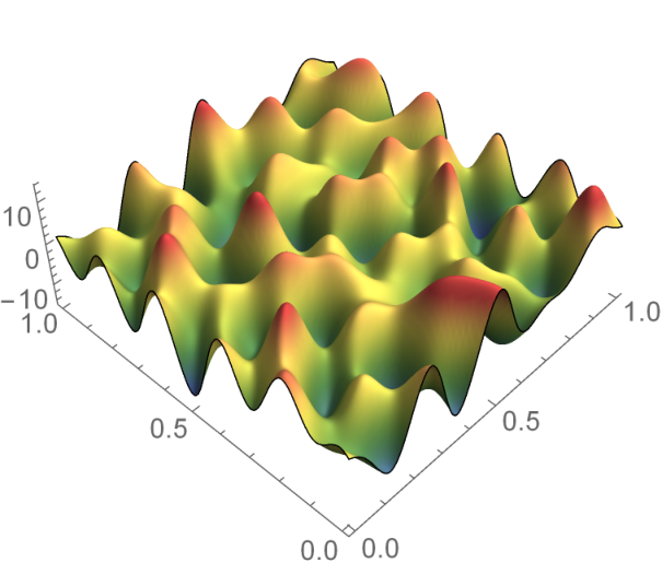
For the filtration we tried to construct -verified grids for thresholds between and using spacings of . Out of the 601 thresholds, we failed to construct -verified grids for 11 thresholds. The largest number of consecutive failures occurred when both and failed to be verified. Hence the largest gap between any two verified thresholds in our filtration was . Therefore the persistent diagrams we calculated are within a bottleneck distance of of the true persistent diagrams for our given function.
The computation took 193 hours and used 16 MB of memory, and was performed on a single Intel i7-2600 processor. The algorithm created a filtered CW structure on which contained 145,721 cells, which was then processed by the Perseus software program to compute its persistent homology [23]. The -approximate filtration was constructed sequentially by computing , so at most three CW complexes were stored in memory at a given time. At the cost of using more memory, one could reduce the computation time by computing the cellular approximations in parallel, and subsequently creating the filtration . Additionally, the one point of departure our implementation took from the algorithm here described is that the cells were represented using a lookup table, as opposed to the product of generalized intervals.
The reason our algorithm failed to verify the thresholds is because when attempting to verify them, it surpassed 25 subdivisions of the domain. In general, the size of geometric features in these sub-level sets was much larger than . However, the error bounds produced by interval arithmetic have a risk of creating a cascade of cubes which fail to become -verified. In order to compute interval arithmetic more precisely, whenever we computed a function on a cube, we subdivided the cube seven times and computed the function using interval arithmetic on each piece.
When we repeated the computation but instead used six subdivisions, the number of thresholds we failed to verify increased fold and the accuracy of our computed persistence diagram was only in the bottleneck distance (it failed to verify seven consecutive thresholds). Using six subdivisions also increased the number of cells in the filtered complex by , however the entire computation finished times faster. We refer the reader to [3, 5] for more efficient techniques to compute precise interval arithmetic bounds needed by this algorithm.
Acknowledgments
The authors would like to thank Konstantin Mischaikow for his insightful comments and conversations.
References
- [1] Gunnar Carlsson, Vin de Silva, and Dmitriy Morozov, Zigzag persistent homology and real-valued functions, Proceedings of the Twenty-fifth Annual Symposium on Computational Geometry (New York, NY, USA), SCG ’09, ACM, 2009, pp. 247–256.
- [2] Frederic Chazal, Vin de Silva, Marc Glisse, and Steve Oudot, The structure and stability of persistence modules, arXiv (2013), 1207.3674.
- [3] Gregory Scott Cochran, Thomas Wanner, and Paweł Dłotko, A randomized subdivision algorithm for determining the topology of nodal sets, Computational Methods in Science and Engineering 35 (2013), no. 5, B1034–B1054.
- [4] David Cohen-Steiner, Herbert Edelsbrunner, and John Harer, Stability of persistence diagrams, Discrete Comput. Geom. 37 (2007), no. 1, 103–120. MR 2279866 (2008i:68130)
- [5] Sarah Day, William D. Kalies, and Thomas Wanner, Verified homology computations for nodal domains, Multiscale Modeling and Simulation 7 (2009), 1695–1726.
- [6] Paweł Dłotko, Tomasz Kaczynski, Marian Mrozek, and Thomas Wanner, Coreduction homology algorithm for regular CW-complexes, Discrete & Computational Geometry 46 (2010), 361–388.
- [7] Herbert Edelsbrunner and John Harer, Persistent homology-a survey, Contemporary mathematics 453 (2008), 257–282.
- [8] Herbert Edelsbrunner and John L. Harer, Computational topology, American Mathematical Society, Providence, RI, 2010, An introduction. MR 2572029 (2011e:00001)
- [9] Marcio Gameiro, Konstantin Mischaikow, and William Kalies, Topological characterization of spatial-temporal chaos, Phys. Rev. E 70 (2004), 035203.
- [10] Marcio Gameiro, Konstantin Mischaikow, and Thomas Wanner, Evolution of pattern complexity in the Cahn-Hilliard theory of phase separation, Acta Materialia 53 (2005).
- [11] Eldon Hansen and G William Walster, Global optimization using interval analysis: revised and expanded, vol. 264, CRC Press, 2003.
- [12] Allen Hatcher, Algebraic topology, Cambridge University Press, 2001.
- [13] J. Jaquette and M. Kramar, C++ code available at: http://chomp.rutgers.edu/Projects/Rigorous_Computational_Dynamics/Approximating_Persistence_Diagrams.html.
- [14] Tomasz Kaczynski, Konstantin Mischaikow, and Marian Mrozek, Computational homology, Springer, 2004.
- [15] L. Kondic, A. Goullet, C.S. O’Hern, M. Kramar, K. Mischaikow, and R.P. Behringer, Topology of force networks in compressed granular media, Europhys. Lett. 97 (2012), 54001.
- [16] M. Kramar, A. Goullet, L. Kondic, and K. Mischaikow, Persistence of force networks in compressed granular media, Phys. Rev. E 87 (2013), 042207.
- [17] by same author, Quantifying force networks in particulate systems, Physica D 283 (2014), 37–55.
- [18] M. Kramar, R. Levanger, M. Shcatz, M. Paul, M. Xu, J. Tithof, B. Suri, and K. Mischaikow, Detecting recurrent dynamics of Kolmogorov flow and Rayleigh-Benard convection, (2014), In preparation.
- [19] Kapilanjan Krishan, Huseyin Kurtuldu, Michael Schatz, Marcio Gameiro, Konstantin Mischaikow, and Santiago Madruga, Homology and symmetry breaking in Rayleigh-Benard convection: Experiments and simulations, Physics of Fluids 19 (2007).
- [20] H. Kurtuldu, K. Mischaikow, and M. F. Schatz, Measuring the departures from the Boussinesq approximation in Rayleigh-Benard convection experiments, Journal of Fluid Mechanics 682 (2011), 543–557.
- [21] R. Mendoza, K. Thornton, I. Savin, and P.W. Voorhees, The evolution of interfacial topology during coarsening, Acta Materialia 54 (2006), 743–750.
- [22] Yuriy Mileyko, Sayan Mukherjee, and John Harer, Probability measures on the space of persistence diagrams, Inverse Problems 27 (2011), no. 12, 124007.
- [23] Konstantin Mischaikow and Vidit Nanda, Morse theory for filtrations and efficient computation of persistent homology, Discrete & Computational Geometry 50 (2013), no. 2, 330–353.
- [24] Konstantin Mischaikow and Thomas Wanner, Topology-guided sampling of nonhomogeneous random processes, Annals of Applied Probability 20 (2010), no. 3, 1068–1097.