CALIBRATION OF THE MIXING-LENGTH THEORY FOR CONVECTIVE WHITE DWARF ENVELOPES
Abstract
A calibration of the mixing-length parameter in the local mixing-length theory (MLT) is presented for the lower part of the convection zone in pure-hydrogen atmosphere white dwarfs. The parameterization is performed from a comparison of 3D CO5BOLD simulations with a grid of 1D envelopes with a varying mixing-length parameter. In many instances, the 3D simulations are restricted to the upper part of the convection zone. The hydrodynamical calculations suggest, in those cases, that the entropy of the upflows does not change significantly from the bottom of the convection zone to regions immediately below the photosphere. We rely on this asymptotic entropy value, characteristic of the deep and adiabatically stratified layers, to calibrate 1D envelopes. The calibration encompasses the convective hydrogen-line (DA) white dwarfs in the effective temperature range (K) and the surface gravity range . It is established that the local MLT is unable to reproduce simultaneously the thermodynamical, flux, and dynamical properties of the 3D simulations. We therefore propose three different parameterizations for these quantities. The resulting calibration can be applied to structure and envelope calculations, in particular for pulsation, chemical diffusion, and convective mixing studies. On the other hand, convection has no effect on the white dwarf cooling rates until there is a convective coupling with the degenerate core below 5000 K. In this regime, the 1D structures are insensitive to the MLT parameterization and converge to the mean 3D results, hence remain fully appropriate for age determinations.
Subject headings
convection – hydrodynamics – stars: evolution – stars: fundamental parameters – stars: interiors – white dwarfsI. INTRODUCTION
In late-type stars, giants, and cool white dwarfs, the convective outer envelope has a significant impact on the observed properties. The physical principles explaining convective energy transport in stars are well understood, although the non-local and turbulent nature of convection has delayed the development of precise models for convective stellar layers. The mixing-length theory [8, hereafter MLT] has proven rather successful despite presenting a very simple description of convection. In this picture, the condition that distinguishes between convective and stable layers is the Schwarzschild criterion, and the convective efficiency, the ratio of convective and radiative fluxes, is computed from local quantities. In the super-adiabatic convective layers that define the atmosphere of most stars, the predicted convective efficiency is very sensitive to the underlying model describing the radiative energy losses, the lifetime, and the geometrical shape of individual convective structures. These quantities are not well constrained by the MLT and must be calibrated from observations.
In recent years, three dimensional (3D) radiation hydrodynamical (RHD) simulations have provided predictions for the surface convection that are in very good agreement with the observed solar granulation [57, see, e.g.,]. Furthermore, various studies relied on 3D RHD simulations to improve the predicted photospheric structures and spectroscopic abundance determinations for the Sun and other stars [1, 10, 44, 45]. In addition to a better representation of the surface inhomogeneities, 3D model atmospheres feature non-local effects, such as the so-called top overshoot layers, which are completely missing in local 1D MLT models [56, 35, 38, 22, 55].
The deep convection zone, where the stratification becomes essentially adiabatic, is not sensitive to the convection model. It is however the entropy jump in the super-adiabatic layers that completely defines the asymptotic entropy value of the deep, adiabatically stratified structure, hence also the depth of the convection zone. One possibility to model these layers is to rely on RHD simulations to determine the asymptotic entropy value for the deep convection zone [48, 34]. This arises from the prediction that upflows formed at the base of the convection zone follow an adiabat almost up to the visible surface [49]. The 1D MLT envelopes are then calibrated from the multi-dimensional asymptotic entropy, a technique that has been employed for late-type stars and giants [34, 36]. The calibrated 1D structures nevertheless neglect the overshoot layers predicted at the base of non-local convection zones [5, 11, 46, 21], which for deep convective envelopes, impacts the convective mixing into the nuclear burning core. In this work, we are interested in the calibration of 1D envelopes of DA white dwarfs with a pure-hydrogen atmosphere. All currently available white dwarf structures rely on the local MLT with a fixed parameterization [51, 19, 41, 42, see, e.g.,].
Surface granulation in DA white dwarfs is qualitatively very similar to that seen in the Sun and stars [54], albeit with shorter lifetimes and smaller characteristic sizes, which are roughly inversely proportional to gravity. Convective instabilities due to hydrogen recombination develop in the atmosphere of these pure-hydrogen stellar remnants at K, although convective energy fluxes only become significant at K for . The convection zone eventually grows to sub-photospheric, and essentially adiabatic layers, at slightly lower effective temperatures. White dwarfs in the range (K) have super-adiabatic photospheric layers where the 1D MLT parameterization has a strong influence on the predicted thermal structures and spectra [3, 33, 4]. Tremblay et al. [55] recently demonstrated that the local 1D MLT is unable to reproduce the mean photospheric structure of 3D simulations, and that shortcomings in the 1D MLT are responsible for the spurious high values previously derived from spectroscopic observations of cool convective white dwarfs [2]. In particular, the top overshoot region was found to have a crucial impact on the spectroscopic predictions.
The convection zone in DA white dwarfs remains limited to the thin hydrogen envelope until it reaches the degenerate core at K, or mixes with the underlying helium layer if the total gravitationally stratified mass of hydrogen is less than about [51]. Before one of these events takes place, the cooling process is regulated by the radiative interface layer just above the largely isothermal degenerate core, which is in some sense the bottle-neck for the energy transport. The evolutionary calculations converge to the so-called radiative zero solution, hence they are insensitive to the details of the convection model [17], which is unlike earlier evolutionary stages [20, see, e.g.,]. The situation is different below K, where the cooling rates are directly impacted by the convecting coupling between the interior thermal reservoir and the radiating surface. In this temperature range, however, the super-adiabatic peak has a negligible amplitude, or in other words, the full convection zone has an essentially adiabatic structure which does not depend on the MLT parameterization. As a consequence, the cooling ages predicted from current 1D evolutionary sequences are not expected to be impacted by 3D effects. However, the convection zone has an indirect effect on observed ages, since they are often derived from spectroscopically determined atmospheric parameters that are modified by 3D effects.
There are a number of cases where 3D effects on structures are expected to have a direct impact. Non-adiabatic pulsation calculations depend critically on the structure of the convective layers, especially for the determination of the edges of the ZZ Ceti instability strip of pulsating DA white dwarfs [18, 26, 27]. Chemical diffusion applications [39, 40, 15] and convective mixing studies [13, see, e.g.,] also depend critically on the size and especially the dynamical properties of the convection zone, e.g. the root-mean-square (RMS) vertical velocity in the convective overshoot layers at the base of the convection zone [21]. In order to characterize white dwarfs accreting disrupted planets, it is likely important to account for the currently neglected convective overshoot [32]. The total mass of the chemical elements mixed in the convection zone (hereafter mixed mass), and to a lesser degree their relative abundances, depend on how rapidly these elements diffuse in the deep overshoot region. Through the remaining of this work, overshoot refers only to the region at the base of the convection zone, since the top overshoot layers have no direct relevance for white dwarf envelope and structure models.
This study proposes a calibration of the MLT free parameters for the size of the convection zone in 1D envelopes of DA white dwarfs from a comparison with CO5BOLD 3D simulations previously computed for spectroscopic applications [55]. We emphasize that our proposed calibration has little in common with the spectroscopic parameterization of the MLT. In both cases, the free parameters of the MLT are employed to mimic specific properties of the mean 3D simulations and mean 3D spectra, respectively, rather than to describe the more general underlying nature of convection. In Section 2, we introduce our grid of 3D simulations and 1D envelope models. We follow in Section 3 with definitions for the sizes of non-local convection zones. In Section 4, we compare 1D and 3D models in order to propose and discuss a MLT parameterization in Section 5. We conclude in Section 6.
II. WHITE DWARF MODELS
II.1. 3D Model Atmosphere Simulations
We rely on CO5BOLD 3D simulations that were presented in earlier works [53, 54, 55, hereafter TL13a, TL13b, and TL13c, respectively]. The 70 simulations cover the range (K) and (see Appendix A of TL13c). While TL13c reviewed the predicted spectral properties drawn from these simulations, which mostly depend on the uppermost regions of the convection zone, the study presented here reports on the overall properties and lower parts of convection zones. The natural starting point is therefore the comparison of 3D and 1D structures at presented in TL13a. We have demonstrated that sequences at different surface gravities possess rather similar properties (TL13b, TL13c), largely because 3D effects depend mostly on the local density, and the same range of densities is found at all surface gravities, albeit with a shift in .
The numerical setup of the 3D model atmospheres is described in detail in TL13a, and more broadly in Freytag et al. [23] in terms of the general properties of the code. We provide a brief overview in this section. The 3D simulations rely on an equation-of-state (EOS) and opacity tables that are computed with the same microphysics as that of standard 1D model atmospheres [52]. We employed a grid of points in the and directions, where is used for the vertical direction and points towards the exterior of the star. The grid spacing in the direction is non-equidistant and the total horizontal extent is chosen in order to have about 10 granules at the surface. The structure of the deep convection zone is largely determined by the radiative energy losses in the photosphere, which also fix the of a simulation. As suggested by Brassard & Fontaine [9], Hansen [29], and Fontaine et al. [19], non-gray atmospheres are an essential boundary condition for precise envelope calculations. The 3D simulations solve the non-gray radiative transfer using 8 to 13 opacity bins, which has proven adequate for spectroscopic applications (TL13c). This setup is likely more than sufficient for a comparison with 1D structure calculations which are less sensitive to the optically thin layers.
The implementation of boundary conditions is described in detail in Freytag et al. [23, see Sect. 3.2]. In brief, the lateral boundaries are periodic, and the top boundary is open to material flows and radiation. We rely on bottom conditions that are either open or closed to convective flows. The lower boundary is closed (hereafter closed simulations) when the vertical extent of the convection zone can be fully included in the simulation. This is the situation for the 3D simulations with , and 14,000 K, for 7.0, 7.5, 8.0, 8.5, and 9.0, respectively. In those cases, we impose zero vertical velocities at the bottom, and a radiative flux is injected from below.
For cooler simulations, the bottom layer is open to convective flows and radiation (hereafter open simulations), and a zero total mass flux is enforced. We specify the entropy of the ascending material to obtain approximately the desired value (an indirect quantity computed from the resulting emergent flux of the simulation). Figure 1 shows that the entropy from 1D envelopes (see Sect. 2.3) at the lower boundary of the convection zone increases monotonically with . Convection is essentially adiabatic in deep convection zones, and the entropy value in the lower part of the convection zone is assumed to be the same as that of the upflows at the bottom of the simulations (see Sect. 2.2).

In all models, the top boundary reaches a space- and time-averaged value of no more than a Rosseland optical depth of . The bottom layer was generally fixed at , well below the photosphere, i.e. the line-forming regions. A few models were extended to deeper layers when the bottom of the convection zone was too close to the simulation boundary. We cover at least 3 pressure scale heights () below the unstable regions when the bottom of the simulation is closed to mass flows.
II.2. Properties of the Deep Convection Zone
The physical conditions at the bottom of convection zones can be extracted from 3D simulations even if we do not simulate the full zones. We rely on the technique presented in Ludwig et al. [34], for which a demonstration is shown in Figure 2 for a DA simulation at K and . We present the local 3D values of the entropy in convective structures (black dots) as a function of geometrical depth with the stellar surface on the right-hand side. We also display the average entropy profile over constant geometrical depth (solid red line). We observe significant entropy fluctuations at all depths, although there is a constant asymptotic upper limit, hereafter . According to the scenario developed in Stein & Nordlund [49] and Ludwig et al. [34], the gas in central regions of broad ascending flows is still thermally isolated from its surroundings until it reaches layers immediately below the photosphere. In other words, convective upflows keep an imprint of the physical conditions at the bottom of the convection zone. The averaged 3D entropy, on the other hand, is not a conserved quantity due to radiative losses and the presence of downdrafts created in the photosphere.
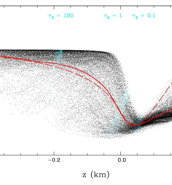
The above technique only applies if the center of upflows remains adiabatic, hence a minimum requirement is that the conditions at the bottom of the convection zone are adiabatic. We have observed that the adiabatic transition takes place when the bottom of the convection zone reaches layers deeper than . For all of our simulations with an open bottom, we can recover an asymptotic value. For closed simulations, there is no significant entropy plateau since conditions are never adiabatic, although in those cases we can directly extract the properties at the bottom of the convection zones.
We also overlay in Figure 2 the 1D model atmosphere with the MLT calibrated from a comparison of with a grid of 1D envelopes (see Section 4.2). The 1D model atmospheres and envelopes calibrated is this way are only meant to recover the conditions at the bottom of the convection zone, although by construction they also provide an accurate mean structure for the essentially adiabatic parts of the convection zone. On the other hand, there is no guarantee that the calibrated 1D models will provide a good match to the mean 3D stratification in super-adiabatic layers. Fortunately, in the case of white dwarfs in contrast to main-sequence stars, the super-adiabatic layers have little direct impact on applications that require the use of 1D envelopes. As it was custom until now, it is generally sufficient to employ 1D envelopes where the MLT parameterization is based on the deep layers, and rely on a different set of models, e.g. 3D simulations, for atmospheric parameter determinations. An inspection of Figure 2 demonstrates that if needed, a connection of the 1D and mean 3D structures at large depth could also be a fairly good approximation.
II.3. 1D Envelope Models
For the purpose of this work, we computed 1D envelopes relying on the MLT for the treatment of convection, similar to those presented in Fontaine et al. [19] and van Grootel et al. [27]. The models employ the ML2 treatment of MLT convection [7, 51] and an EOS for a non-ideal pure-hydrogen gas [43]. Realistic non-gray temperature gradients are extracted from detailed atmospheric computations and employed as upper boundary conditions [9, 27]. The non-gray effects on the size of the convection zone are shown in Figure 5 of van Grootel et al. [27]. In order to compare the envelopes to 3D simulations, we have varied the mixing length to pressure scale height ratio11 1 ML2/ has the same functional form as the more commonly used for stars but it also specifies the choice of auxiliary parameters of the MLT formulation [34]. ML2/ from values of 0.4 to 2.0 in steps of 0.2. ML2/ is selected as a proxy for all MLT free parameters since changes in the other parameters have similar effects on the structures. We use the same range of surface gravities and (steps of 0.5 dex and 100 K, respectively) as our set of 3D calculations.

From the 1D envelopes we have extracted the physical conditions at the bottom of the convection zone. Figure 3 depicts the hydrogen mass integrated from the surface (), with respect to the total white dwarf mass, for the case. Clearly, the MLT parameterization has a strong effect on the size and mass included in the convection zone at intermediate temperatures, where the atmospheric layers are super-adiabatic.
To ensure that we share a common entropy zero point in all calculations, we computed all entropy values using the same EOS as the 3D simulations, based on the Hummer & Mihalas [31] non-ideal EOS, where we have also accounted for partial degeneracy. The entropy values at the bottom of the convection zone are shown in Figure 1 (solid lines), along with additional sequences where we have neglected partial degeneracy (dotted lines). The degeneracy effects are very small in the convection zone (, where is the chemical potential of the free electrons). This is largely due to the fact that the degeneracy level is constant for an adiabatic process. For the essentially adiabatic structure of cool white dwarf convection zones, degeneracy is changing very slowly as a function of depth [6, see Eq. (13) of]. Furthermore, degeneracy effects are still negligible at the lower limit where the calibration of ML2/ is performed in this work (see Section 5.1).
Our proposed calibration of the MLT is performed by comparing 3D simulations to 1D envelopes. We also rely on 1D MLT model atmospheres [52] for illustrative purposes in cases where we display a detailed comparison of 1D and mean 3D stratifications as a function of depth. The 1D model atmospheres and envelopes provide very similar results, within a few percent, below the photosphere.
III. DEFINITION OF CONVECTIVE LAYERS
In the following, we rely on mean 3D values, hereafter , for all quantities except for the asymptotic entropy . values are the temporal and spatial average of 3D simulations over constant geometrical depth. We use 250 snapshots in the last 25% of a simulation to make the temporal average. While our earlier studies have relied on averages over constant optical depth, the geometrical depth is better suited to extract convective fluxes and overshoot velocities.
Before comparing 3D simulations and 1D envelopes, it is crucial to define what we refer to as the convection zone. In the local MLT picture, the convective regions are clearly characterized as the layers where the radiative gradient
| (1) |
is larger than the adiabatic gradient
| (2) |
with the temperature and the pressure. All other parts of the structure are fully static. This is a rather crude approximation of the dynamical nature of convection, where material flows do not vanish abruptly when the thermal structure becomes stable. In this section, we review the different regions that are found in non-local models of the lower part of convection zones [46, 12, 21, see also]. Table 1 formally defines the regions discussed in this section, and we give an example of the geometrical extent and mass included in these layers based on the 12,100 K and simulation.
| Region | aaThe coordinate points towards the exterior of the star. | aaThe coordinate points towards the exterior of the star. | bbRanges are taken from the simulation at K and as an illustrative example. Zones 3 and 4 feature an exponential decay of (negative) flux and velocity, respectively, and their depth can only be defined approximately. For the example presented here, we adopt a bottom boundary of for Zone 3. | bbRanges are taken from the simulation at K and as an illustrative example. Zones 3 and 4 feature an exponential decay of (negative) flux and velocity, respectively, and their depth can only be defined approximately. For the example presented here, we adopt a bottom boundary of for Zone 3. | |||||
|---|---|---|---|---|---|---|---|---|---|
| (3D) | (1D) | (3D) | (1D) | (3D) | (1D) | ||||
| Zone 1 | |||||||||
| Zone 2 | 0.2 | ||||||||
| Zone 3 | |||||||||
| Zone 4 |
To further illustrate the profile of 3D convection zones, Figure 4 displays the RMS vertical velocities for closed-box simulations at . We start from the vertical velocity
| (3) |
where the mass flux weighted mean velocity (second term on right-hand side) is removed from the directly simulated velocity to account for the residual numerical mass flux. The latter results from the presence of plane-parallel oscillations and an imperfect temporal averaging due to the finite number of snapshots. The corresponding RMS vertical velocity is
| (4) |
where all averages are performed over constant geometrical depth22 2 This differs from the RMS velocity fluctuation where is expected to be non-zero due to a correlation between velocity and density fluctuations in the convection zone.. Furthermore, Figures 5 and 6 show the and 1D convective flux profiles. The convective flux is the sum of the enthalpy and kinetic energy fluxes,
| (5) |
where is the internal energy per gram, the density, and the 3D velocity. The mass flux weighted energy flux (third term on right-hand side of Eq. (5)) is subtracted to correct for any residual non-zero mass flux in the numerical simulations as in Eq. (4). This correction is a small fraction of the convective flux for all simulations. The total energy is defined from
| (6) |
We use the logarithm of the temperature as an independent variable since it is a local quantity, while optical depth and mass are integrated from the top of the convection zone, and are more sensitive to differences in the photosphere.


The proper convection zone in 3D (open circles in Figs. 4-6) is defined in the same way as in 1D from the Schwarzschild (stability) criterion. In this region, the entropy gradient is negative with respect to geometrical depth (increasing towards the exterior). In the following, we define the bottom of this region as the Schwarzschild boundary. In the 3D simulations, convective flows are largely created, horizontally advected, and merged into narrow downdrafts in the photosphere [21]. Large entropy fluctuations are produced by the radiative cooling in these layers, which drives the convective motions. For cool convective white dwarfs ( K, ) with deep convection zones, entropy fluctuations are smaller in the photosphere and the dominant role of the downflows is diminished. The descending fluid form a hierarchical structure of merging downdrafts due to the increase of the pressure scale height with depth [1].
In the 3D simulations, downdrafts at the base of the convection zone (according to the Schwarzschild criterion) still have large momenta. They are also denser than the ambient medium, albeit with a decreasing difference. As a consequence, the convective cells are still accelerated in the region just below the unstable layers. Mass conservation guarantees that there is warm material transported upwards, hence there is a positive convective flux is this region. These layers are equivalent to a convection zone in thermodynamical terms. We define the bottom of this region as the layer where and refer to it as the flux boundary (filled circles in Figs. 4-6). The typical size of the region between the Schwarzschild and flux boundaries is a bit less than one pressure scale height, or 0.3 dex in mass.
At the flux boundary, the momentum of the downdrafts remains significant, hence they penetrate into even deeper layers. This is the beginning of the convective overshoot region, although some authors prefer the term convective penetration [58] when the convective flux is still energetically relevant. In these layers, convective structures are decelerated since they have a density deficit. Downdrafts are generally warmer than the ambient medium and they carry a net downwards (negative) convective flux, or in other words, the temperature gradient in these layers is larger than the radiative gradient. That follows from the change of sign of the velocity-enthalpy correlation. However, Figure 5 demonstrates that this negative overshoot flux is always a small fraction () of the total flux. Once the convective flux has decreased by one order of magnitude, or to a value of less than 1% of the total flux, the energetic impact on the structure becomes very small.
The negative convective flux and velocities decay in a similar exponential way below the flux boundary, both with a scale height close to . While the convective flux becomes rapidly energetically negligible, the convective velocities still have mixing capabilities in much deeper layers. This situation is due to the extreme ratio between convective and diffusive time scales (see Section 5.2). In typical cases for DA white dwarfs, convective velocities are of the order of km s-1 at base of the convection zone, while overshoot velocities of the order of 1 m s-1 still dominate over the slower diffusive speeds, and can efficiently mix elements [21]. This implies that microscopic diffusion timescales are likely to dominate only in the deep overshoot layers, i.e. a few below the flux boundary. The exact layer where this happens depends on the diffusing trace chemical element and the atmospheric parameters of the model, although it is clear that the mixed region can be much larger than in the 1D approximation. In Figures 4-6, we identify the position of a 1 dex velocity decay with respect to the velocity at the flux boundary (filled triangles), which is generally close to the bottom of the simulation. Our simulations evidently provide a truncated picture of the overshoot layers and we review this issue in Section 5.2.
IV. COMPARISON OF 1D AND 3D CONVECTION ZONES
IV.1. Closed 3D Simulations
We first proceed with a direct comparison of and 1D stratifications in the case of shallow convection zones, completely enclosed within the simulation domain. Figures 7 and 8 present the logarithmic values of the temperature and pressure, respectively, characterizing the bottom of the convection zone for simulations at . We rely on three different definitions for the size of the convection zone as discussed in Section 3, with the same symbols as in Figures 4-6. These regions correspond to the Schwarzschild boundary (open circles), the flux boundary (filled circles), and a decay of 1 dex (open triangles) below the reference value at the flux boundary. Figures 7 and 8 also display 1D sequences, with values ranging from ML2 = 0.4 to 2.0 in steps of 0.2, using the Schwarzschild boundary to define the size of the convection zone (solid lines).


Figures 7 and 8 demonstrate that the 1D envelope that best matches the bottom of a 3D simulation is generally independent of whether the matching is performed on temperature or pressure. The pressure is proportional to the 1D mass column, where only thermodynamic pressure contributes to hydrostatic equilibrium, while in 3D simulations one must also account for the turbulent pressure. Figure 3 depicts the and 1D comparison in terms of the hydrogen mass, and the results are similar to those presented for the temperature and pressure at the base of the convection zone. It implies that even though and 1D models have different profiles in the photosphere, due to the top convective overshoot and turbulent pressure, differences in the integrated mass column are small in the lower part of the convection zone. In the following, the calibrated ML2 is the average value of the two 1D models that best match the pressure and temperature at the bottom of the convection zone, respectively, within a prescribed boundary. The mass column can be directly extracted from the envelopes calibrated in this way.
In terms of the Schwarzschild boundary, Figures 7 and 8 demonstrate that the mixing-length parameter increases rapidly with , with values of 0.88, 1.07, and 1.32 at 12,100, 12,500, and 13,000 K, respectively. In this range partially covering the ZZ Ceti instability strip, the MLT variation is significant compared to the usually assumed constant value of ML2/ = 1.0 for envelopes [16]. Our calibration of ML2/ is meant to represent the temperature and pressure at the Schwarzschild boundary, and by construction, it provides an estimation of the average temperature gradient for the full convection zone. However, the photospheric temperature gradient of a calibrated 1D envelope is not expected to correspond to that of the 3D simulation.
For the convection zone defined in terms of the flux boundary, ML2/ values have to be increased to 1.00, 1.25, and 1.50 for the same values as above. The derived efficiency is significantly higher than that found for the Schwarzschild boundary. One should be cautious since an inspection of Figure 5 for 1D model atmospheres calibrated for the flux boundary (blue dashed lines) reveals that while the zero point of convective flux is by definition in agreement with the 3D simulations, the overall shape of the convective flux is not very well reproduced for shallow convection zones. Our calibration of ML2/ is mostly useful to characterize the depth at which convection becomes energetically insignificant and the velocities start to decay exponentially with geometrical depth. Finally, Figure 9 demonstrates that the versus 1D results (temperature only) at other gravities are fairly similar, albeit with a shift in . As a consequence, the previous discussion applies most generally to white dwarfs with shallow convection zones.

For the very warm simulations, e.g. 13,500 and 14,000 K at = 8.0, the Schwarzschild and flux boundaries are essentially in the photosphere (), and therefore the ML2/ value for these layers becomes coupled with the MLT parameterization used in spectroscopic applications (TL13c). Both 3D simulations and 1D models show new patterns in this regime. The convective flux becomes negligible outside of the unstable layers, and there is a reversal of the flux and Schwarzschild boundaries, with the Schwarzschild boundary moving below the flux boundary with increasing . In this regime, efficient radiation transport is able to smooth temperature fluctuations. This diminishes the flux of internal energy (first term in Eq. (5)) over a shorter distance from the top of the convection zone than the velocity field becomes symmetric in up- and downflows. The significant momentum of the narrow downdrafts produces a negative kinetic energy flux (second term in Eq. (5)). This flux remains large near the mean Schwarzschild boundary since cool downdrafts get convectively stable at larger geometrical depths than the upflows. As a consequence, the mean total flux becomes negative slightly above the mean Schwarzschild boundary. We have verified that there is no reversal of the flux and Schwarzschild boundaries when the kinetic energy flux is neglected. The MLT does not account for the kinetic energy flux, hence we do not expect a similar reversal in 1D.
For convective 1D models at large , the size of the unstable regions becomes insensitive to the MLT parameterization according to Figure 7, hence it is not possible to calibrate the MLT based on the Schwarzschild boundary. This picture is somewhat misleading since the MLT convective fluxes, and associated velocities, remain very sensitive to the value of the MLT parameters. Figure 7 shows that the 1D convective flux drops to very small values (, dotted lines) much higher in the photosphere than the 1D Schwarzschild boundary.
Our results would naively suggest that convective efficiency increases with but the 3D simulations present a more complex picture. At high , non-local effects from strong and deep reaching downdrafts create flux profiles that are extended and smoother as a function of geometrical depth than in the 1D case, both at the top and bottom of the convection zone. In Figure 10, we have calibrated ML2/ in order to reproduce the maximum value of the convective flux, which peaks in the photosphere, for shallow convection zones. Clearly, a much smaller mixing-length parameter is necessary to match the convective flux in the photosphere in comparison to the Schwarzschild or flux boundaries. The values of ML2/ = 0.6-0.8 are consistent with the commonly used spectroscopic parameterizations (TL13c). Nevertheless, the parameterizations for the Schwarzschild and flux boundaries offer a better representation of the conditions at the bottom of the convection zones.

We have already discussed the fact that the convection zone is drastically deeper when defined in terms of the convective velocities. This is also seen in Figures 7 and 8 where we show the position of the one order of magnitude decrease for below the flux boundary (open triangles). It is inappropriate to parameterize the 1D MLT for the highly non-local overshoot velocities, and it would produce spurious stratifications in the unstable regions. Instead, we propose an overshoot parameterization that does not directly involve the MLT in Section 5.2.
IV.2. Open 3D Simulations
For open 3D simulations, we have extracted the asymptotic entropy values characterizing the deep adiabatic layers using the technique described in Section 2.2. is directly derived from the specified entropy of the ascending material at the bottom boundary of the simulations. We have verified that this matches the observed asymptotic value below the photosphere (see, e.g., Figure 2). We then assume that also corresponds to the entropy value at the bottom of the unstable layers in 1D envelopes. The and 1D entropy values are compared in Figure 1 for the case. The calibration of ML2/ is directly performed from a match of with entropy values interpolated from the grid of 1D envelopes. In Figure 3, we show the resulting hydrogen mass integrated from the surface.
At low temperatures ( K at ), DA white dwarfs have extremely small super-adiabatic atmospheric layers, and the structure remains essentially adiabatic from the bottom to the top of the convection zone. Since the top of the convection zone is higher than the photosphere (), the effective temperature directly identifies the entropy value at the bottom of the convection zone. The choice of the MLT parameterization does not matter since there is no significant radiative energy exchange during one advective (turnover) timescale.
V. DISCUSSION
V.1. 1D MLT Calibration
Figure 11 (top panel) presents the MLT parameterization for the lower part of the convection zone in order to recover the Schwarzschild boundary (hereafter ML2/) of the 70 3D simulations in our grid. We illustrate with different symbols the calibration derived directly from closed 3D simulations (open circles) and inferred from a match of (filled squares). We also present in Figure 11 (bottom panel) the calibration matching the flux boundary (hereafter ML2/). The latter calibration is directly performed for closed simulations, and in those cases, is 16% larger than with a relatively small dispersion of 3%. Therefore, we simply assume that ML2/ for open 3D simulations. This is likely a good approximation in the transition region between closed and open 3D simulations, and at lower , the 1D envelopes depend less critically on the MLT parameterization.

The calibration is not performed when the 1D mass included within the convection zone varies by an amount smaller than 0.2 dex for the range of ML2 between 0.4 and 2.0. This defines the upper and lower boundaries in Figure 11, which depend on . At the cool end, we propose to keep ML2/ constant, since the value is irrelevant for structure calculations. Similarly, at values above those in the calibration range, it is likely acceptable to keep the value constant for most applications. The choice of the asymptotic ML2/ value is not obvious, however, because of its rapid variation with . As a compromise, we adopt values of 1.2 and 1.4, for ML2/ and ML2/, respectively, at values larger than our calibration range. If one is interested in the detailed properties of shallow convection zones above K at = 8.0, it may be preferable to combine the and 1D structures at some depth below the convection zone where the convective flux is negligible. The MLT does not reproduce very well the extended but inefficient 3D convection zones in this regime. For values above our calibration range, most of the 3D effects will be from the overshoot at the base of the convection zone since contrary to the small convective fluxes, velocities remain significant well below the photosphere.
Table 2 provides the tabulated MLT parameterizations, which are valid for 1D envelopes with an EOS, opacities, and boundary conditions similar to those employed for our grid. Physical conditions at the bottom of our calibrated envelopes (mass, temperature, and pressure) are also given as a reference point. Moreover, we propose fitting functions for ML2/ and ML2/, respectively, where the independent variables are defined as
| (7) |
| (8) |
and the functions are as follow with numerical coefficients found in Table 3
| (9) |
| (10) |
The proposed functions are presented in Figure 11 along with the data points. Similarly to our 3D atmospheric parameter corrections in TL13c, we have adopted functions that do not retain the fine details of the 3D and 1D differences. Small scale fluctuations may be due to inaccuracies in the grid of 3D simulations. Ultimately, the calibrated 1D structures do not provide the detailed convective flux profile and neglect the turbulent nature of convection. It is not well constrained how much these 3D effects impact chemical diffusion and pulsation calculations. Finally, we remind the reader that 1D structure codes typically make approximations for the non-gray radiative transfer in the atmospheres, which may introduce a slight offset in the size of convection zones. The ML2/ offset is at most a few percent for our setup (see Section 2.3). As a consequence, we believe that a calibration within 5% is sufficient.
| ML2/ aaCorresponds to the position of the Schwarzschild boundary for closed simulations (see Section 4.1). For open simulations, the calibration is performed by matching the 3D value with the 1D entropy at the bottom of the convection zone (see Section 4.2). | aaCorresponds to the position of the Schwarzschild boundary for closed simulations (see Section 4.1). For open simulations, the calibration is performed by matching the 3D value with the 1D entropy at the bottom of the convection zone (see Section 4.2). | aaCorresponds to the position of the Schwarzschild boundary for closed simulations (see Section 4.1). For open simulations, the calibration is performed by matching the 3D value with the 1D entropy at the bottom of the convection zone (see Section 4.2). | aaCorresponds to the position of the Schwarzschild boundary for closed simulations (see Section 4.1). For open simulations, the calibration is performed by matching the 3D value with the 1D entropy at the bottom of the convection zone (see Section 4.2). | ML2/ bbCorresponds to the position of the flux boundary for closed simulations. For open simulations, we simply assume that ML2/ (see Section 5.1). | bbCorresponds to the position of the flux boundary for closed simulations. For open simulations, we simply assume that ML2/ (see Section 5.1). | bbCorresponds to the position of the flux boundary for closed simulations. For open simulations, we simply assume that ML2/ (see Section 5.1). | bbCorresponds to the position of the flux boundary for closed simulations. For open simulations, we simply assume that ML2/ (see Section 5.1). | ||
|---|---|---|---|---|---|---|---|---|---|
| (K) | [K] | [dyn cm-2] | [K] | [dyn cm-2] | |||||
| 6112 | 7.00 | 0.53 | 6.06 | 5.93 | 14.04 | 0.61 | 6.03 | 5.94 | 14.07 |
| 7046 | 7.00 | 0.53 | 6.79 | 5.80 | 13.30 | 0.61 | 6.74 | 5.81 | 13.36 |
| 8027 | 7.00 | 0.63 | 7.51 | 5.68 | 12.58 | 0.74 | 7.42 | 5.69 | 12.67 |
| 9025 | 7.00 | 0.69 | 8.90 | 5.41 | 11.19 | 0.80 | 8.69 | 5.45 | 11.40 |
| 9521 | 7.00 | 0.70 | 10.14 | 5.17 | 9.94 | 0.81 | 9.78 | 5.24 | 10.31 |
| 10018 | 7.00 | 0.69 | 12.00 | 4.84 | 8.07 | 0.80 | 11.49 | 4.93 | 8.59 |
| 10540 | 7.00 | 0.72 | 13.92 | 4.44 | 6.16 | 0.85 | 13.33 | 4.58 | 6.74 |
| 11000 | 7.00 | 1.05 | 14.30 | 4.34 | 5.78 | 1.20 | 13.98 | 4.42 | 6.10 |
| 11501 | 7.00 | 1.20 | 14.63 | 4.28 | 5.45 | 1.40 | 14.59 | 4.29 | 5.49 |
| 12001 | 7.00 | 1.20 | 14.78 | 4.26 | 5.30 | 1.40 | 14.77 | 4.26 | 5.30 |
| 12501 | 7.00 | 1.20 | 14.89 | 4.24 | 5.19 | 1.40 | 14.89 | 4.24 | 5.19 |
| 13003 | 7.00 | 1.20 | 14.98 | 4.23 | 5.10 | 1.40 | 14.98 | 4.23 | 5.10 |
| 6065 | 7.50 | 0.58 | 6.91 | 5.90 | 14.17 | 0.67 | 6.90 | 5.90 | 14.19 |
| 7033 | 7.50 | 0.58 | 7.54 | 5.79 | 13.54 | 0.67 | 7.51 | 5.80 | 13.57 |
| 8017 | 7.50 | 0.58 | 8.22 | 5.68 | 12.86 | 0.68 | 8.16 | 5.69 | 12.92 |
| 9015 | 7.50 | 0.66 | 9.07 | 5.53 | 12.01 | 0.77 | 8.95 | 5.55 | 12.13 |
| 9549 | 7.50 | 0.71 | 9.83 | 5.38 | 11.25 | 0.82 | 9.64 | 5.42 | 11.44 |
| 10007 | 7.50 | 0.70 | 10.81 | 5.19 | 10.27 | 0.81 | 10.52 | 5.25 | 10.55 |
| 10500 | 7.50 | 0.70 | 12.30 | 4.93 | 8.78 | 0.82 | 11.86 | 5.00 | 9.21 |
| 10938 | 7.50 | 0.74 | 13.68 | 4.68 | 7.40 | 0.86 | 13.12 | 4.79 | 7.96 |
| 11498 | 7.50 | 0.94 | 14.79 | 4.42 | 6.29 | 1.09 | 14.27 | 4.56 | 6.81 |
| 11999 | 7.50 | 1.20 | 15.24 | 4.32 | 5.84 | 1.40 | 15.06 | 4.36 | 6.02 |
| 12500 | 7.50 | 1.20 | 15.43 | 4.29 | 5.65 | 1.40 | 15.42 | 4.29 | 5.66 |
| 13002 | 7.50 | 1.20 | 15.53 | 4.28 | 5.55 | 1.40 | 15.52 | 4.28 | 5.55 |
| 5997 | 8.00 | 0.52 | 7.68 | 5.89 | 14.40 | 0.60 | 7.67 | 5.89 | 14.41 |
| 7011 | 8.00 | 0.52 | 8.44 | 5.75 | 13.64 | 0.60 | 8.42 | 5.76 | 13.65 |
| 8034 | 8.00 | 0.52 | 9.01 | 5.66 | 13.07 | 0.60 | 8.97 | 5.67 | 13.11 |
| 9036 | 8.00 | 0.61 | 9.66 | 5.55 | 12.41 | 0.71 | 9.58 | 5.57 | 12.50 |
| 9518 | 8.00 | 0.64 | 10.10 | 5.47 | 11.98 | 0.74 | 9.98 | 5.50 | 12.10 |
| 10025 | 8.00 | 0.69 | 10.71 | 5.36 | 11.36 | 0.80 | 10.56 | 5.39 | 11.52 |
| 10532 | 8.00 | 0.68 | 11.61 | 5.19 | 10.46 | 0.79 | 11.39 | 5.23 | 10.68 |
| 11005 | 8.00 | 0.72 | 12.63 | 5.00 | 9.45 | 0.84 | 12.32 | 5.06 | 9.75 |
| 11529 | 8.00 | 0.76 | 14.04 | 4.76 | 8.04 | 0.88 | 13.58 | 4.84 | 8.50 |
| 12099 | 8.00 | 0.88 | 15.27 | 4.51 | 6.81 | 1.00 | 14.82 | 4.63 | 7.26 |
| 12504 | 8.00 | 1.07 | 15.69 | 4.40 | 6.38 | 1.25 | 15.27 | 4.52 | 6.81 |
| 13000 | 8.00 | 1.20 | 16.05 | 4.33 | 6.03 | 1.40 | 15.96 | 4.35 | 6.12 |
| 13502 | 8.00 | 1.20 | 16.18 | 4.31 | 5.89 | 1.40 | 16.17 | 4.31 | 5.90 |
| 14000 | 8.00 | 1.20 | 16.26 | 4.30 | 5.81 | 1.40 | 16.26 | 4.30 | 5.82 |
| 6024 | 8.50 | 0.60 | 8.51 | 5.86 | 14.57 | 0.70 | 8.51 | 5.86 | 14.57 |
| 6925 | 8.50 | 0.60 | 9.32 | 5.71 | 13.76 | 0.70 | 9.31 | 5.72 | 13.76 |
| 8004 | 8.50 | 0.60 | 9.80 | 5.65 | 13.28 | 0.70 | 9.78 | 5.65 | 13.30 |
| 9068 | 8.50 | 0.60 | 10.38 | 5.55 | 12.69 | 0.70 | 10.33 | 5.56 | 12.74 |
| 9522 | 8.50 | 0.64 | 10.67 | 5.51 | 12.41 | 0.74 | 10.61 | 5.52 | 12.47 |
| 9972 | 8.50 | 0.66 | 11.01 | 5.45 | 12.07 | 0.76 | 10.93 | 5.46 | 12.14 |
| 10496 | 8.50 | 0.68 | 11.52 | 5.35 | 11.55 | 0.79 | 11.41 | 5.38 | 11.67 |
| 10997 | 8.50 | 0.74 | 12.19 | 5.23 | 10.89 | 0.86 | 12.04 | 5.26 | 11.04 |
| 11490 | 8.50 | 0.72 | 13.04 | 5.08 | 10.04 | 0.84 | 12.81 | 5.12 | 10.26 |
| 11979 | 8.50 | 0.73 | 14.09 | 4.89 | 8.99 | 0.84 | 13.78 | 4.95 | 9.29 |
| 12420 | 8.50 | 0.76 | 15.11 | 4.72 | 7.96 | 0.88 | 14.68 | 4.79 | 8.40 |
| 12909 | 8.50 | 0.84 | 16.11 | 4.50 | 6.96 | 0.95 | 15.71 | 4.61 | 7.37 |
| 13453 | 8.50 | 1.08 | 16.47 | 4.42 | 6.61 | 1.28 | 16.10 | 4.51 | 6.97 |
| 14002 | 8.50 | 1.19 | 16.76 | 4.36 | 6.31 | 1.40 | 16.67 | 4.38 | 6.41 |
| 14492 | 8.50 | 1.20 | 16.89 | 4.33 | 6.18 | 1.40 | 16.87 | 4.34 | 6.20 |
| 6028 | 9.00 | 0.70 | 9.38 | 5.80 | 14.70 | 0.81 | 9.38 | 5.80 | 14.70 |
| 6960 | 9.00 | 0.70 | 10.24 | 5.67 | 13.84 | 0.81 | 10.23 | 5.67 | 13.84 |
| 8041 | 9.00 | 0.70 | 10.75 | 5.59 | 13.33 | 0.81 | 10.74 | 5.60 | 13.34 |
| 8999 | 9.00 | 0.70 | 11.10 | 5.55 | 12.98 | 0.81 | 11.09 | 5.55 | 12.99 |
| 9507 | 9.00 | 0.71 | 11.34 | 5.51 | 12.74 | 0.82 | 11.31 | 5.52 | 12.77 |
| 9962 | 9.00 | 0.72 | 11.59 | 5.47 | 12.48 | 0.84 | 11.56 | 5.48 | 12.52 |
| 10403 | 9.00 | 0.71 | 11.89 | 5.42 | 12.18 | 0.82 | 11.85 | 5.43 | 12.23 |
| 10948 | 9.00 | 0.67 | 12.37 | 5.34 | 11.70 | 0.77 | 12.30 | 5.35 | 11.78 |
| 11415 | 9.00 | 0.71 | 12.84 | 5.25 | 11.23 | 0.83 | 12.73 | 5.27 | 11.35 |
| 11915 | 9.00 | 0.76 | 13.47 | 5.14 | 10.61 | 0.88 | 13.33 | 5.16 | 10.75 |
| 12436 | 9.00 | 0.72 | 14.32 | 4.99 | 9.76 | 0.84 | 14.11 | 5.03 | 9.97 |
| 12969 | 9.00 | 0.73 | 15.29 | 4.83 | 8.79 | 0.85 | 15.02 | 4.87 | 9.06 |
| 13496 | 9.00 | 0.82 | 16.05 | 4.70 | 8.03 | 0.96 | 15.75 | 4.75 | 8.32 |
| 14008 | 9.00 | 0.89 | 16.92 | 4.51 | 7.15 | 1.03 | 16.52 | 4.62 | 7.56 |
| 14591 | 9.00 | 1.17 | 17.23 | 4.44 | 6.85 | 1.40 | 16.87 | 4.53 | 7.20 |
| 14967 | 9.00 | 1.20 | 17.47 | 4.38 | 6.61 | 1.40 | 17.34 | 4.41 | 6.73 |
Note. — is the spatial and temporal average of the emergent flux. The RMS variations are found in Table 1 of TL13b. , , and are extracted at the bottom of the convection zone from calibrated 1D envelopes.
| Coefficient | ML2/ | ML2/ |
|---|---|---|
| a1 | 1.1989083E+00 | 1.4000539E+00 |
| a2 | 1.8659403E+00 | 5.1134694E01 |
| a3 | 1.4425660E+00 | 1.1159288E+00 |
| a4 | 6.4742170E02 | 1.0083984E+00 |
| a5 | 2.9996192E02 | 5.7427026E02 |
| a6 | 6.0750771E02 | 5.4884977E+00 |
| a7 | 5.2572772E02 | 1.6106825E02 |
| a8 | 5.4690218E+00 | 7.5656008E03 |
| a9 | 1.6330177E01 | 6.8772823E02 |
| a10 | 2.8348941E01 | 2.9166886E01 |
| a11 | 1.7353691E+01 | 1.8977236E+01 |
| a12 | 4.3545950E01 | 3.6544167E01 |
| a13 | 2.1739157E01 | 2.2859657E01 |
V.2. Parameterization of Overshoot Velocities
We have so far neglected the convective overshoot below the flux boundary. In most cases, the quantity of interest is the overshoot velocity, which does not exist in the local MLT. In the following, we aim at providing a parameterization for overshoot in regions below the 1D convection zone.
The spatial scales and timescales involved in convection and microscopic diffusion differ by many orders of magnitude in typical white dwarfs. It is therefore not possible for multi-dimensional simulations to model both effects simultaneously. Instead, we depict the far overshoot regime as a random walk process characterized by a macroscopic diffusion coefficient, which simply counter-balances the microscopic diffusion coefficient in 1D calculations. The mixed regions are those where macroscopic diffusion dominates over microscopic diffusion. Freytag et al. [21] studied this random walk process with tracer particles in 2D RHD simulations. They found that the particles are immediately mixed within the convection zone, but that the RMS vertical spread in the overshoot layers could be described from
| (11) |
where is the macroscopic diffusion coefficient
| (12) |
with a characteristic timescale. Just based on MLT models or even with detailed RHD simulations, is not directly available for the deep overshoot regions of interest. As a consequence, Freytag et al. [21] propose, from a match to 2D simulations and physical considerations, that has an exponential decay below the convection zone. The resulting diffusion coefficient then takes the form
| (13) |
where is the velocity at the base of the convection zone and the velocity scale height. In the following, we assume that the base of the convection zone is the flux boundary as determined by 3D simulations and the 1D ML2 parameterization.
V.2.1 Closed 3D Simulations
For closed 3D simulations, it is possible to verify the proposed exponential decay of overshoot velocities, as well as calibrate Eq. (13) by extracting , , and . Figure 12 demonstrates that over the three pressure scale heights typically included in our simulations below the flux boundary, the velocity decay is nearly exponential. The velocity scale height is very close to one pressure scale height (dotted black line), although it is actually changing with depth. It is larger than one pressure scale height immediately below the flux boundary, and becomes subsequently smaller. As a consequence, taking is very likely to overestimate macroscopic diffusion in the deep overshoot layers, and gives an upper limit to the mixed mass. Finally, Freytag et al. [21] demonstrate that the timescale of overshoot for shallow convection zones is the same as the characteristic convective timescale in the photosphere, since this is where the downdrafts are formed. As a consequence, it is possible to use directly the characteristic granulation timescales computed in TL13b and TL13c. In Table 4, we present at the flux boundary () and the characteristic granulation timescales () for closed simulations, which can be used in Eq. (13) for shallow convection zones. The velocity scale height can be directly evaluated from the 1D pressure scale height in the envelopes since this quantity is not significantly impacted by 3D effects, although we also include the local values at the base of the convection zone in Table 4.

The overshoot coefficients in Table 4 are limited by the range of our 3D simulations. Figure 13 compares the maximum velocities, which peak slightly below the photosphere, for and 1D ML2/ = 0.7 models at . We applied the MLT parameterization that best represents the maximum convective flux of the warmest 3D simulations (see Figure 10 and TB13c). The MLT suggests that velocities in the photosphere for (K) are still of the same order of magnitude as in cooler models, although the upper limit depends critically on the MLT parameterization. The large photospheric velocities are likely to support strong overshoot layers in DA white dwarfs above our warmest 3D simulations, even though convection has a negligible effect on the thermal structure.

| aaCorresponds to at the flux boundary. | bbSame as the decay time in Table A.1 of TL13c. | ccCorresponds to at the flux boundary. | ||
|---|---|---|---|---|
| (K) | (105 cm s-1) | [s] | [cm] | |
| 10540 | 7.00 | 3.36 | 0.28 | 5.30 |
| 11000 | 7.00 | 3.31 | 0.21 | 5.34 |
| 11501 | 7.00 | 3.52 | 0.29 | 5.50 |
| 12001 | 7.00 | 2.74 | 0.43 | 5.54 |
| 12501 | 7.00 | 1.56 | 0.49 | 5.55 |
| 13003 | 7.00 | 0.95 | 0.46 | 5.51 |
| 11498 | 7.50 | 3.27 | 0.50 | 4.81 |
| 11999 | 7.50 | 3.24 | 0.67 | 4.91 |
| 12500 | 7.50 | 3.10 | 0.86 | 5.04 |
| 13002 | 7.50 | 2.60 | 1.05 | 5.10 |
| 12099 | 8.00 | 3.33 | 0.96 | 4.45 |
| 12504 | 8.00 | 3.14 | 0.95 | 4.35 |
| 13000 | 8.00 | 3.04 | 1.15 | 4.47 |
| 13502 | 8.00 | 2.75 | 1.30 | 4.56 |
| 14000 | 8.00 | 1.88 | 1.37 | 4.59 |
| 12909 | 8.50 | 3.21 | 1.48 | 3.98 |
| 13453 | 8.50 | 2.92 | 1.44 | 3.89 |
| 14002 | 8.50 | 2.70 | 1.54 | 3.99 |
| 14492 | 8.50 | 2.49 | 1.68 | 4.08 |
| 14008 | 9.00 | 3.06 | 1.81 | 3.48 |
| 14591 | 9.00 | 2.71 | 1.85 | 3.41 |
| 14967 | 9.00 | 2.47 | 1.92 | 3.47 |
V.2.2 Open 3D Simulations
For open 3D simulations, we can not directly extract quantities to calibrate Eq. (13). Furthermore, the assumption that the overshoot timescale is the same as the surface granulation timescale is unlikely to be valid, since the downdrafts have time for merging into the hierarchical structure observed in simulations of deep, convective envelopes [38]. We propose instead that , with the velocity scale height equal to the pressure scale height as above. Therefore, is the only quantity that remains to be evaluated.
For deep and essentially adiabatic convection zones, the MLT and 3D simulations agree on the temperature gradient. An examination of the MLT equations demonstrates that for very efficient convection (), velocity is proportional to , along with a dependence on heat capacity and molecular weight in the presence of partial ionization. While the 1D velocity model is only an idealization of the complex 3D dynamics, we suggest that the ratio remains very similar across the deep convection zone. This is seen in Figure 4 for the cooler 10,025 K model where convection is reasonably adiabatic below the photosphere. Figure 14 shows the versus 1D ML2 velocity ratio for open simulations and a reference layer identified by the criterion . This region is deep enough for convection to be largely adiabatic, and far away from the bottom boundary to prevent numerical effects. We observe small variations around a mean value of = 1.5 for the DA white dwarfs with a deep adiabatic convection zone. We suggest that this calibration remains valid down to the bottom of the convection zone, as long as . We still face the problem, however, that by definition . We recommend instead to take a characteristic velocity one pressure scale height above the bottom of the convection zone. In summary, for the range below the one covered by Table 4, we propose the following overshoot parameterization
| (14) |
where all quantities are extracted from 1D ML2 structures as described above.

We confirm the results of Freytag et al. [21] that overshoot is significant and present for all DA white dwarfs with convectively unstable layers ( K). The total mass of hydrogen included in the overshoot region may be a few orders of magnitude greater than the mass included in the proper convection zone. This effect is totally neglected in local MLT models, and our proposed parameterization provides an order of magnitude estimate (upper limit) of the overshoot velocities and macroscopic diffusion coefficients. The resulting effects on the chemical abundances of mixed elements, for instance in accreting white dwarfs in a steady state, depend on the outcomes of chemical diffusion calculations.
V.3. Improvements to the Local MLT
The previous sections have revealed that the local MLT only depicts a rough portrait of the underlying dynamical nature of convection, which is illustrated by the need of having different parameterizations for different applications. We note that non-local 1D MLT models could provide a better match to the 3D results. In particular, the models discussed in Spiegel [47], Skaley & Stix [46], Dupret et al. [14], and Stökl [50] naturally deliver the Schwarzschild and flux boundaries, as well as (partial) overshoot layers. In these non-local MLT models, the more realistic physics is recovered at the expense of adding more free parameters. In some sense, this is a more elegant and accurate way of obtaining the Schwarzschild and flux boundaries than we have proposed in this work. While it does require some modifications of existing 1D model atmosphere and structure codes, this should be investigated in the future.
Montgomery & Kupka [37] have also presented a non-local convection model for white dwarfs, although in this case it is not an extension of the MLT theory. However, one issue for all non-local 1D models discussed here is that they have not been very successful at modeling overshoot velocities reproducing the exponential decay observed in RHD simulations, which is the main part of the 1D models that we would like to improve.
V.4. ZZ Ceti Instability Strip
The spectroscopically determined atmospheric parameters of pulsating ZZ Ceti white dwarfs have been discussed in TL13c, as seen in the light of our grid of spectra. We found that the dominant 3D effect is on the spectroscopically determined surface gravity, with an average shift of = 0.1 for ZZ Ceti stars in the sample of Gianninas et al. [25]. On the other hand, 3D corrections depend critically on the calibration of the MLT parameters in the reference 1D model atmospheres. Based on the 1D ML2/ = 0.8 calibration, we observed a 3D shift of = 225 K on average, although this is in the same range as the uncertainties in the 3D corrections. The spectroscopic blue edge at , below which white dwarfs are pulsating, is located at K when relying on spectra, while it is slightly warmer by 100 K based on 1D ML2/ = 0.8 model atmospheres. On the other hand, the red edge is located at K for . Overall, the observed position of the instability strip is not changed significantly compared to earlier investigations [24, 25]. We remind the reader that the observed edges are defined from only a few pulsating and constant objects, and that the individual errors on the spectroscopic atmospheric parameters must also be considered.
Non-adiabatic asteroseismic models provide predictions for the position of the blue edge of the ZZ Ceti instability strip, although the results are highly sensitive to the parameterization of convection [18, 26]. Recently, van Grootel et al. [27] relied on a non-adiabatic code including time-dependent convection to study the driving mechanism. Compared to earlier studies [16, and references therein], their approach neither assumes frozen convection nor an instantaneous convection response during a pulsation cycle. Using 1D ML2/ = 1.0 white dwarf structures similar to those discussed in this work, they find a seismic blue edge at K for . Since the convective flux contribution is critical in the non-adiabatic perturbation equations, we can compare their results with our ML2/ calibration in Figure 11. We find that ML2/ 1.0 at 12,000 K and , in very close agreement with the value generally used to predict the blue edge of the instability strip, based on seismic models. There seems to be a slight discrepancy between the observed and predicted blue edges, the latter being cooler by about K. We note, however, that the current agreement is still fairly good considering the uncertainties in the 3D simulations and spectroscopically determined atmospheric parameters. It would be interesting to review the non-adiabatic pulsation calculations with the new calibrated 1D envelopes or a direct use of the convective flux profiles [26]. Finally, dynamical convection effects that are missing from both current and newly calibrated 1D envelopes could also have an impact on pulsations [27].
At the red edge of the instability strip, van Grootel et al. [28] recently revived an idea of Hansen et al. [30] originally applied to the blue edge. They suggest that the red edge of the g-mode instabilities is reached when the thermal timescale in the driving region (bottom of the convection zone) becomes of the order of the pulsation period. Beyond this limit, outgoing g-waves are no longer reflected back by the atmospheric layers, and will lose their energy in the upper atmosphere. Using this argument for g-modes of spherical-harmonic degree = 1, the red edge lies at 11,000 K for with ML2/ = 1.0 1D envelopes. In this range of , we predict a slightly shallower 3D convection zone, although it is unlikely to impact in a qualitative way the results presented in van Grootel et al. [28].
VI. CONCLUSION
We have presented a comparison of our grid of 3D RHD simulations for 70 DA white dwarfs, in the range , with 1D envelope models based on the mixing-length theory for convection. While MLT only provides a bottom boundary of the convection zone based on the Schwarzschild criterion, the 3D stratifications are more complex. In 3D simulations, convective structures are still accelerated just before reaching the Schwarzschild boundary and the convective flux remains significant in layers below the classical definition of the convection zone. In addition, we confirm that DAs have strong lower overshoot layers, where vertical velocities decay exponentially with a velocity scale height of the order of the pressure scale height.
We proposed two functions to calibrate ML2/ values in 1D envelopes that best reproduce the 3D Schwarzschild and flux boundaries, respectively, as a function of and . The calibration was performed from a direct comparison for closed simulations with shallow convection zones. For cool white dwarfs with deep convection zones, the 3D simulations use an open bottom boundary condition, and therefore do not include the lower part of the convection zone. We rely on the fact that below the atmosphere, upflows still evolve under adiabatic conditions. We have extracted the 3D asymptotic entropy values that correspond to the conditions in the lower part of the convection zones, which were then employed to calibrate ML2/ of 1D MLT envelopes.
We have found that for shallow and inefficient convection zones ( K at ), the MLT parameters for the bottom of the convection zone poorly reproduce the overall convective flux profile through the convection zones. Mean 3D stratifications should be used for studies that require detailed convective flux profiles. For applications such as chemical diffusion and convective mixing, the dominant convective effect is likely to come from the overshoot velocities, which are completely missing from local MLT envelopes. The extreme ratio between convective and microscopic diffusion timescales prohibits the usage of 3D simulations to precisely calibrate the deep overshoot layers. Instead, we reintroduce in the context of white dwarfs the analytical overshoot parameterization initially proposed by Freytag et al. [21], with new constraints based on the 3D simulations. The next step will be to apply our calibrations to non-adiabatic pulsation models as well as specific cases of white dwarfs with convection zones contaminated by metals accreted from former disrupted planets.
References
- [1] Asplund, M., Grevesse, N., Sauval, A. J., & Scott, P. 2009, ARA&A, 47, 481
- [2] Bergeron, P., Wesemael, F., Fontaine, G., & Liebert, J. 1990, ApJ, 351, L21
- [3] Bergeron, P., Wesemael, F., & Fontaine, G. 1992, ApJ, 387, 288
- [4] Bergeron, P., Wesemael, F., Lamontagne, R., et al. 1995, ApJ, 449, 258
- [5] Böhm, K.-H. 1963, ApJ, 138, 297
- [6] Böhm, K.-H. 1968, Ap&SS, 2, 375
- [7] Böhm, K. H., & Cassinelli, J. 1971, A&A, 12, 21
- [8] Böhm-Vitense, E. 1958, ZAp, 46, 108
- [9] Brassard, P., & Fontaine. G. 1997, in White dwarfs, ed. J. Isern, M. Hernanz, & E. Garcia-Berro (Dordrecht: Kluwer Academic Publishers), 214, 451
- [10] Caffau, E., Ludwig, H.-G., Steffen, M., Freytag, B., & Bonifacio, P. 2011, Sol. Phys., 268, 255
- [11] Chan, K. L., & Sofia, S. 1989, ApJ, 336, 1022
- [12] Chan, K. L., & Gigas, D. 1992, ApJ, 389, L87
- [13] Chen, E. Y., & Hansen, B. M. S. 2011, MNRAS, 413, 2827
- [14] Dupret, M.-A., Goupil, M.-J., Samadi, R., Grigahcène, A., & Gabriel, M. 2006, in Proceedings of SOHO 18/GONG 2006/HELAS I, Beyond the spherical Sun, ed. M. Thompson (Noordwijk, ESA), 624, 78
- [15] Dupuis, J., Fontaine, G., Pelletier, C., & Wesemael, F. 1993, ApJS, 84, 73
- [16] Fontaine, G., & Brassard, P. 2008, PASP, 120, 1043
- [17] Fontaine, G., & van Horn, H. M. 1976, ApJS, 31, 467
- [18] Fontaine, G., Brassard, P., Wesemael, F., & Tassoul, M. 1994, ApJ, 428, L61
- [19] Fontaine, G., Brassard, P., & Bergeron, P. 2001, PASP, 113, 409
- [20] Freytag, B., & Salaris, M. 1999, ApJ, 513, L49
- [21] Freytag, B., Ludwig, H.-G., & Steffen, M. 1996, A&A, 313, 497
- [22] Freytag, B., Allard, F., Ludwig, H.-G., Homeier, D., & Steffen, M. 2010, A&A, 513, A19
- [23] Freytag, B., Steffen, M., Ludwig, H.-G., et al. 2012, Journal of Computational Physics, 231, 919
- [24] Gianninas, A., Bergeron, P., & Fontaine, G. 2006, AJ, 132, 831
- [25] Gianninas, A., Bergeron, P., & Ruiz, M. T. 2011, ApJ, 743, 138
- [26] Gautschy, A., Ludwig, H.-G., & Freytag, B. 1996, A&A, 311, 493
- [27] van Grootel, V., Dupret, M.-A., Fontaine, G., et al. 2012, A&A, 539, A87
- [28] van Grootel, V., Fontaine, G., Brassard, P., & Dupret, M.-A. 2013, ApJ, 762, 57
- [29] Hansen, B. M. S. 1999, ApJ, 520, 680
- [30] Hansen, C. J., Winget, D. E., & Kawaler, S. D. 1985, ApJ, 297, 544
- [31] Hummer, D. G., & Mihalas, D. 1988, ApJ, 331, 794
- [32] Koester, D. 2009, A&A, 498, 517
- [33] Koester, D., Allard, N. F., & Vauclair, G. 1994, A&A, 291, L9
- [34] Ludwig, H.-G., Freytag, B., & Steffen, M. 1999, A&A, 346, 111
- [35] Ludwig, H.-G., Allard, F., & Hauschildt, P. H. 2002, A&A, 395, 99
- [36] Ludwig, H.-G., Caffau, E., & Kučinskas, A. 2008, In IAU Symp. 252, ed. L. Deng & K. L. Chan (Cambridge: Cambridge Univ. Press), 75
- [37] Montgomery, M. H., & Kupka, F. 2004, MNRAS, 350, 267
- [38] Nordlund, Å., Stein, R. F., & Asplund, M. 2009, Living Reviews in Solar Physics, 6, 2
- [39] Paquette, C., Pelletier, C., Fontaine, G., & Michaud, G. 1986, ApJS, 61, 197
- [40] Pelletier, C., Fontaine, G., Wesemael, F., Michaud, G., & Wegner, G. 1986, ApJ, 307, 242
- [41] Renedo, I., Althaus, L. G., Miller Bertolami, M. M., et al. 2010, ApJ, 717, 183
- [42] Salaris, M., Cassisi, S., Pietrinferni, A., Kowalski, P. M., & Isern, J. 2010, ApJ, 716, 1241
- [43] Saumon, D., Chabrier, G., & van Horn, H. M. 1995, ApJS, 99, 713
- [44] Scott, P., Grevesse, N., Asplund, M., et al. 2014a, arXiv:1405.0279
- [45] Scott, P., Asplund, M., Grevesse, N., Bergemann, M., & Sauval, A. J. 2014b, arXiv:1405.0287
- [46] Skaley, D., & Stix, M. 1991, A&A, 241, 227
- [47] Spiegel, E. A. 1963, ApJ, 138, 216
- [48] Steffen, M. 1993, in Inside the stars, ed. W. Weiss & A. Baglin, (San Francisco, ASP), 40, 300
- [49] Stein, R. F., & Nordlund, A. 1989, ApJ, 342, L95
- [50] Stökl, A. 2008, A&A, 490, 1181
- [51] Tassoul, M., Fontaine, G., & Winget, D. E. 1990, ApJS, 72, 335
- [52] Tremblay, P.-E., Bergeron, P. & Gianninas, A. 2011, ApJ, 730, 128
- [53] Tremblay, P.-E., Ludwig, H.-G., Steffen, M., & Freytag, B. 2013a, A&A, 552, A13 (TL13a)
- [54] Tremblay, P.-E., Ludwig, H.-G., Freytag, B., Steffen, M., & Caffau, E. 2013b, A&A, 557, A7 (TL13b)
- [55] Tremblay, P.-E., Ludwig, H.-G., Steffen, M., & Freytag, B. 2013c, A&A, 559, A104 (TL13c)
- [56] Unno, W. 1957, ApJ, 126, 259
- [57] Wedemeyer-Böhm, S., & Rouppe van der Voort, L. 2009, A&A, 503, 225
- [58] Zahn, J.-P. 1991, A&A, 252, 179