A Weakly Asymptotic Preserving Low Mach Number Scheme for the Euler Equations of Gas Dynamics Thanks: S.N. is supported by the DFG under grants number NO 361/3-2 and GSC 111. A.B. and M.L. are supported by the DFG under grant number LU 1470/2-2. K.R.A. was supported by the Alexander-von-Humboldt Foundation through a postdoctoral fellowship (2011-12). C.-D.M. is supported by the DFG in the Cluster of Excellence ”Simulation Technology” and SFB TRR 40

S. Noelle ^†^†thanks: Institut für Geometrie und Praktische Mathematik, RWTH-Aachen, Templergraben 55, D-52056 Aachen, Germany. noelle@igpm.rwth-aachen.de G. Bispen ^†^†thanks: Institut für Mathematik, Johannes Gutenberg-Universität Mainz, Staudingerweg 9, D-55099 Mainz, Germany.bispeng@mathematik.uni-mainz.de K. R. Arun ^†^†thanks: School of Mathematics, Indian Institute of Science Education and Research Thiruvananthapuram, India.arun@iisertvm.ac.in M. Lukáčová-Medviďová ^†^†thanks: Institut für Mathematik, Johannes Gutenberg-Universität Mainz, Staudingerweg 9, D-55099 Mainz, Germany. lukacova@mathematik.uni-mainz.de C.-D. Munz ^†^†thanks: Institut für Aerodynamik und Gasdynamik, Universität Stuttgart, Pfaffenwaldring 21, D-70550 Stuttgart, Germany. munz@iag.uni-stuttgart.de

Abstract

We propose a low Mach number, Godunov-type finite volume scheme for the numerical solution of the compressible Euler equations of gas dynamics. The scheme combines Klein’s non-stiff/stiff decomposition of the fluxes (J. Comput. Phys. 121:213-237, 1995) with an explicit/implicit time discretization (Cordier et al., J. Comput. Phys. 231:5685-5704, 2012) for the split fluxes. This results in a scalar second order partial differential equation (PDE) for the pressure, which we solve by an iterative approximation. Due to our choice of a crucial reference pressure, the stiff subsystem is hyperbolic, and the second order PDE for the pressure is elliptic. The scheme is also uniformly asymptotically consistent. Numerical experiments show that the scheme needs to be stabilized for low Mach numbers. Unfortunately, this affects the asymptotic consistency, which becomes non-uniform in the Mach number, and requires an unduly fine grid in the small Mach number limit. On the other hand, the CFL number is only related to the non-stiff characteristic speeds, independently of the Mach number. Our analytical and numerical results stress the importance of further studies of asymptotic stability in the development of AP (asymptotic preserving) schemes.

AMS

[2010] Primary 35L65, 76N15, 76M45; Secondary 65M08, 65M06

keywords

Euler equations of gas dynamics, low Mach number limit, stiffness, semi-implicit time discretization, flux decomposition, asymptotic preserving schemes

26. August 2014

1 Introduction

We consider the non-dimensionalised compressible Euler equations for an ideal gas, which may be written as a system of conservation laws in $d=1,2$ or $3$ space dimensions,

U_{t}+\nabla\cdot F(U)=0,

(1)

where $t>0$ and $\mathbf{x}\in\mathbb{R}^{d}$ are the time and space variables, $U\in\mathbb{R}^{d+2}$ is the vector of conserved variables and $F(U)\in\mathbb{R}^{(d+2)\times d}$ , the flux vector. Here,

U=\begin{pmatrix}\rho\\ \rho\mathbf{u}\\ \rho E\end{pmatrix},\ F(U)=\begin{pmatrix}\rho\mathbf{u}\\ \rho\mathbf{u}\otimes\mathbf{u}+\frac{p}{\varepsilon^{2}}\,\mathbf{Id}\\ (\rho E+p)\mathbf{u}\end{pmatrix},

(2)

with density $\rho$ , velocity $\mathbf{u}$ , momentum $\rho\mathbf{u}$ , total specific energy $E$ , total energy $\rho E$ and pressure $p$ . The operators $\nabla,\nabla\cdot,\otimes$ are respectively the gradient, divergence and tensor product in $\mathbb{R}^{d}$ . The parameter $\varepsilon$ is the reference Mach number and is usually given by

\varepsilon:=\frac{u_{\mathrm{ref}}}{\sqrt{p_{\mathrm{ref}}/\rho_{\mathrm{ref}}}},

(3)

where the basic reference values $\rho_{\mathrm{ref}},u_{\mathrm{ref}}$ , $p_{\mathrm{ref}}$ and length $x_{\mathrm{ref}}$ are problem dependent characteristic numbers. It has to be noted that the reference Mach number $\varepsilon$ is a measure of compressibility of the fluid. Throughout this paper we follow the convention that $0<\varepsilon\leq 1$ and $\varepsilon=1$ corresponds to the fully compressible regime. On the other hand, if the values of the reference parameters are prescribed in such a way that $\varepsilon>1$ , then we redefine them to get $\varepsilon=1$ . This can be achived, e.g. by setting $u_{\mathrm{ref}}=p_{\mathrm{ref}}=\rho_{\mathrm{ref}}=1$ .

The system (1) is closed by the dimensionless equation of state

p=(\gamma-1)\left(\rho E-\frac{\varepsilon^{2}}{2}\rho\lVert\mathbf{u}\rVert^{2}\right),

(4)

with $\gamma>1$ being the ratio of specific heats. As long as the pressure $p$ remains positive, (1) is hyperbolic and the eigenvalues in direction $\mathbf{n}$ are

\lambda_{1}=\mathbf{u}\cdot\mathbf{n}-\frac{c}{\varepsilon},\quad\lambda_{2}=\mathbf{u}\cdot\mathbf{n},\quad\lambda_{3}=\mathbf{u}\cdot\mathbf{n}+\frac{c}{\varepsilon},

(5)

where $c=\sqrt{(\gamma p)/\rho}$ . Therefore, the sound speed $c/\varepsilon$ becomes very large, $\mathcal{O}(\varepsilon^{-1})$ , as the Mach number $\varepsilon$ becomes small, while the advection speed $\mathbf{u}$ remains finite. The spectral condition number of the flux Jacobian becomes proportional to $1/\epsilon$ and numerical difficulties will occur. If acoustic effects can be neglected, then the physical time scale is given by $t_{ref}=x_{\mathrm{ref}}/u_{\mathrm{ref}}$ . For an explicit time discretization, the Courant-Friedrichs-Lewy condition (CFL number) imposes a numerical time step $\Delta t$ that has to be proportional to $\varepsilon$ . Hence, the numerical time step has to be much smaller than the physical one and becomes intolerable for $\varepsilon\ll 1$ .

There is an abundance of literature on the computation of low Mach number weakly compressible and incompressible flows. A pioneering contribution is due to Chorin [5] who introduced the projection method for incompressible flows via an artificial compressibility. In [27], Turkel introduced the well known pre-conditioning approach to reduce the stiffness of the problem. In the case of unsteady weakly compressible problems, Klein [19] derives a multiple pressure variables approach using low Mach number asymptotic expansions. Klein’s work was later extended to both inviscid and viscous flow problems by Munz and collaborators, see, e.g. [23, 26]. The review paper [20] gives a good survey of the recent develops on the asymptotic based low Mach number approximations and further references on this subject.

This paper aims to contribute to two well known, challenging issues: First, we propose and analyse a scheme which is based upon Klein’s non-stiff/stiff splitting [19]. We combine this with an explicit/implicit time discretization due to Cordier, Degond and Kumbaro [6], which transforms the stiff energy equation into a second order nonlinear PDE for the pressure. Due to our choice of reference pressure, both the non-stiff and the stiff subsystems are hyperbolic. The implicit terms in the stiff system are reduced to a second order elliptic PDE for the pressure and is solved at every time step by an iterative approximation. This procedure allows a CFL number which is only bounded by the advection velocity (i.e. it is independent of the Mach number $\varepsilon$ ).

The second issue is related to Klainerman and Majda’s celebrated result that solutions to the compressible Euler equations converge to the solutions of the incompressible Euler equations as the Mach number tends to zero. Jin [17] introduced a related consistency criterion for numerical schemes: a scheme is asymptotic preserving (AP), if its lowest order multiscale expansion is a consistent discretization of the incompressible limit; see the equations (10)-(12). An AP scheme for the low Mach number limit of the Euler equations should serve as a consistent and stable discretization, independent the Mach number $\varepsilon$ . In the fully compressible regime, i.e. when $\varepsilon=\mathcal{O}(1)$ , the AP scheme should have the desirable features of a compressible solver, such as non-oscillatory solution profiles and good resolution of shock type discontinuities. On the other hand, the AP scheme should yield a consistent discretization of the incompressible equations when $\varepsilon\to 0$ . We refer the reader to [1, 2, 6, 8, 14] and the references cited therein for some AP schemes for the Euler equations and other related applications. In Section 3.3 we prove that our scheme possess the AP property.

While Klein’s paper motivated strongly such a pressure-based approach, in which the pressure is used as a primary variable, Guillard and Viozat [13] proposed a further development of the pre-conditioning technique based on the low Mach number asymptotic analysis. The question with respect to efficiency of this density-based approach in comparison to the pressure-based has no clear answer. The pressure-based solver has its advantage especially in the low Mach number regime due to the splitting of stiff and non-stiff terms. All the implicit treatment of the stiff terms is reduced to a scalar elliptic equation for the pressure. For small Mach numbers such a pressure-based approach is usually used in commercial codes. In the fully compressible regime the pressure-based approach has the restriction of the implicit treatment of the sonic terms even for $M>1$ , which may be no longer necessary. The density-based approach has the advantage that it starts from a typical compressible solver as used in aerodynamics to get a steady state. Hence, we expect that it will be the best approach for larger Mach numbers. At small Mach numbers, the preconditioning reduces the sound speed of the system to avoid the stiffness in the equations. By a dual time stepping technique it may be extended to unsteady flows. Hence, for very small Mach numbers the density-based approach should be more difficult - the $M=0$ case can not be handeled.

The rest of this paper is organised as follows. Section 2 contains several preliminaries: in Section 2.1 we briefly recall the asymptotic analysis as well as the incompressible limit due to Klainerman and Majda [18]. In Section 2.2 we recall Klein’s flux splitting and introduce our choice of reference pressure. In Section 2.3 we prove that the non-stiff subsystem respects the structure of divergence-free velocity and constant pressure fields. This property helps to avoid spurious initial layers for low Mach number computations.

In Section 3 we introduce our time discretization and prove the AP property: in Section 3.1, we propose the first order scheme IMEX scheme. In Section 3.2 we derive the nonlinear elliptic pressure equation and discuss an iterative linearization to solve it. In Section 3.3 we prove the AP property for this scheme. In Section 3.4 we define a second-order time discretization based on the Runge-Kutta Crank-Nicolson (RK2CN) scheme. At this point our scheme is not uniformly asymptotically stable with respect to $\varepsilon$ . Indeed, for some test problems, the scheme is only stable if $\Delta t=O(\varepsilon\Delta x)$ . Therefore, we introduce a fourth order pressure stabilization in Section 3.5. We prove asymptotic consistency in Theorem 14. While the ratio $\Delta t/\Delta x$ is now independent of $\varepsilon$ , we need to restrict both $\Delta t$ and $\Delta x$ as the Mach number goes to zero as $\Delta t=O(\varepsilon^{2/3})=\Delta x$ .

Section 4 describes the fully discrete scheme with spatial reconstruction, numerical fluxes and a linear system solver. In Section 5 we present the numerical experiments.

Finally, we draw some conclusions in Section 6. In particular, we discuss possible ways to analyze and improve asymptotic stability.

2 Asymptotic Analysis and Flux Splitting

In this section we review the asymptotic analysis presented in [18, 19], from which the incompressible limit equations are derived (Subsection 2.1), a splitting of the fluxes into non-stiff and stiff parts with a technique to guarantee the hyperbolicity of the stiff part (Subsection 2.2) and the importance of well-prepared initial data which eliminate spurious initial layers (Subsection 2.3).

2.1 Asymptotic Analysis and Incompressible Limit

In this section we consider the low Mach number limit of the Euler equations (1)-(2), obtained via a formal multiscale asymptotic analysis [18]. Following [19, 22] we use a three-term asymptotic ansatz

f(\mathbf{x},t)=f^{(0)}(\mathbf{x},t)+\varepsilon f^{(1)}(\mathbf{x},t)+\varepsilon^{2}f^{(2)}(\mathbf{x},t)

(6)

for all the flow variables. The ansatz (6) was introduced by Klainerman and Majda [18]. A drawback of this ansatz is that it cannot resolve long wave phenomena, particularly those related to acoustic waves. However, our focus is on resolving slow convective wave, e.g. vortices. In order to resolve long wavelength one has to consider multiple space scales in (6) and multiple pressure variables as [19, 26].

A multiscale analysis consists of inserting the ansatz (6) into the Euler system (1)-(2) and balancing the powers of $\varepsilon$ . This leads to a hierarchy of asymptotic equations which shows the behaviour of the different order terms. In the following, we briefly review the results of multiscale analysis presented in [19, 22].

The leading order terms in the conserved variables do not give a completely determined system of equations. Even though the leading order terms in density and velocity form a coupled system of equations, the presence of second order pressure term makes the system incomplete. Both the leading order and second order pressure terms influence the leading order density and velocity fields. The pressure $p(\mathbf{x},t)$ admits the multiscale representation [19]

p(\mathbf{x},t)=p^{(0)}(t)+\varepsilon^{2}p^{(2)}(\mathbf{x},t).

(7)

Here, the leading order pressure term $p^{(0)}$ allows only temporal variations and $p^{(0)}$ is a thermodynamic variable satisfying the equation of state, i.e.

p^{(0)}=(\gamma-1)(\rho E)^{(0)}.

(8)

As a result of the compression or expansion at the boundaries, the pressure $p^{(0)}$ changes in time and vice-versa, according to the relation

\frac{1}{\gamma p^{(0)}}\frac{dp^{(0)}}{dt}=-\frac{1}{\lvert\Omega\rvert}\int_{\partial\Omega}\mathbf{u}^{(0)}\cdot\mathbf{n}d\sigma.

(9)

As a consequence of (9), it can be inferred that the leading order velocity $\mathbf{u}^{(0)}$ cannot be arbitrary; an application of the Gauss theorem to the right hand side yields a divergence constraint on $\mathbf{u}^{(0)}$ . In the limit $\varepsilon\to 0$ , $p^{(0)}$ becomes a constant and which gives the standard divergence-free condition of incompressible flows.

The first order pressure $p^{(1)}$ is also function of time, independent of $\mathbf{x}$ . However, it can admit long scale variations, say $\mbox{\boldmath$\xi$}=\varepsilon\mathbf{x}$ and $p^{(1)}$ can be thought of as the amplitude of an acoustic wave. Therefore, in order to include the effect of $p^{(1)}$ , instead of (6), one would require a multiple space-scale ansatz in both $\mathbf{x}$ and $\xi$ , cf. [19]. However, in the limit $\varepsilon\to 0$ , the large scale becomes infinite and $p^{(1)}$ becomes constant in space and time; see also [18]. Therefore, in this work we consider only a single space-scale ansatz (6) and thus $p^{(1)}$ is constant in space.

In order to interpret the meaning of the second order term $p^{(2)}$ , we write the classical zero Mach number limit equations, i.e.

$\displaystyle\rho^{(0)}_{t}+\nabla\cdot\left(\rho^{(0)}\mathbf{u}^{(0)}\right)$	$\displaystyle=0,$	(10)
$\displaystyle\left(\rho^{(0)}\mathbf{u}^{(0)}\right)_{t}+\nabla\cdot\left(\rho^{(0)}\mathbf{u}^{(0)}\otimes\mathbf{u}^{(0)}\right)+\nabla p^{(2)}$	$\displaystyle=0,$	(11)
$\displaystyle\nabla\cdot\mathbf{u}^{(0)}$	$\displaystyle=-\frac{1}{\gamma p^{(0)}}\frac{dp^{(0)}}{dt}.$	(12)

We notice that the above zero Mach number equation system has a mixed hyperbolic-elliptic character in contrast to the hyperbolic Euler equations (1)-(2). Here, $p^{(2)}$ survives as the incompressible pressure which is a Lagrange multiplier for the divergence-free constraint (12).

2.2 Flux-splitting into non-stiff and Stiff Parts

Based on the asymptotic structure presented in the previous paragraph, Klein [19] proposed a new splitting of the Euler fluxes and a novel Godunov-type scheme for the low Mach number regime. We refer to [16] for a detailed derivation. The flux-splitting reads

F(U)=\hat{F}(U)+\tilde{F}(U),

(13)

where

\hat{F}(U)=\begin{pmatrix}\rho\mathbf{u}\\ \rho\mathbf{u}\otimes\mathbf{u}+p\,\mathbf{Id}\\ (\rho E+\Pi)\mathbf{u}\end{pmatrix},\ \tilde{F}(U)=\begin{pmatrix}0\\ \frac{1-\varepsilon^{2}}{\varepsilon^{2}}p\,\mathbf{Id}\\ (p-\Pi)\mathbf{u}\end{pmatrix}.

(14)

Here, $\mathbf{Id}$ denotes the $d\times d$ identity matrix and $\Pi=\Pi(\mathbf{x},t)$ is an auxiliary pressure variable which should satisfy

\lim\limits_{\varepsilon\to 0}\Pi(\mathbf{x},t)=p^{(0)}(t),\quad\lim\limits_{\varepsilon\to 1}\Pi(\mathbf{x},t)=p(\mathbf{x},t).

(15)

This is achieved by defining

\Pi(\mathbf{x},t):=\varepsilon^{2}p(\mathbf{x},t)+(1-\varepsilon^{2}){p}_{\infty}(t),

(16)

where the reference pressure $p_{\infty}(t)$ has to satisfy

\lim\limits_{\varepsilon\to 0}p_{\infty}(t)=p^{(0)}(t).

(17)

Remark 1.

We give our choice of $p_{\infty}$ in (26) below.

(i)

The limits (15) respectively (17) and in particular the choice of the reference pressure $p_{\infty}$ play an important role in assuring the correct asymptotic behaviour in the incompressible and compressible regimes respectively; see subsection 3.3 below.
(ii)

Klein chooses

$p_{\infty}(t)=\frac{1}{|\Omega|}\int_{\Omega}p(\mathbf{x},t)d\mathbf{x}.$ (18)

The reference pressure $p_{\infty}$ is related to his so-called ‘nonlocal’ pressure $p_{\mathrm{NL}}$ via

$\displaystyle p_{\mathrm{NL}}(t)$ $\displaystyle=(1-\varepsilon^{2}){p}_{\infty}(t).$ (19)

(iii)

For future reference we note that

\displaystyle p-\Pi=(1-\varepsilon^{2})(p-p_{\infty})

(20)

and hence

\tilde{F}(U)=(1-\varepsilon^{2})\,\begin{pmatrix}0\\[2.15277pt] \frac{p}{\varepsilon^{2}}\,\mathbf{Id}\\[2.15277pt] (p-p_{\infty}){\mathbf{u}}\end{pmatrix}.

(21)

The eigenvalues of the Jacobian of $\hat{F}$ , e.g. in 1-D case, are

\hat{\lambda}_{1}=u-c^{*},\ \hat{\lambda}_{2}=u,\ \hat{\lambda}_{3}=u+c^{*},

(22)

where the ‘pseudo’ sound speed is

c^{*}=\sqrt{\frac{p+(\gamma-1)\Pi}{\rho}}.

(23)

Similarly, the eigenvalues of $\tilde{F}$ are

\tilde{\lambda}_{1}=-\frac{(1-\varepsilon^{2})}{\varepsilon}\sqrt{\frac{(\gamma-1)(p-p_{\infty})}{\rho}},\ \tilde{\lambda}_{2}=0,\ \tilde{\lambda}_{3}=\frac{(1-\varepsilon^{2})}{\varepsilon}\sqrt{\frac{(\gamma-1)(p-p_{\infty})}{\rho}}.

(24)

Note that the eigenvalues of $\hat{F}$ are $\mathcal{O}(1)$ , whereas those of $\tilde{F}$ are $\mathcal{O}(\varepsilon^{-1})$ . Therefore, $\tilde{F}$ represents the ‘stiff’ part of the original flux $F$ and $\hat{F}$ is the corresponding ‘non-stiff’ part.

At this point it might also be noted that the quantity under the square root in the expression for the eigenvalues in (24) need not remain positive, which will destroy the hyperbolicity of the fast system. The crucial point is how to gauge, or equilibrate, the auxiliary pressure $\Pi$ , which is defined only up to a constant. Therefore, instead of taking the average of the pressure to gauge $\Pi$ as in (18), we propose to use the infimum condition

\inf_{\mathbf{x}}\Pi(\mathbf{x},t)=\inf_{\mathbf{x}}p(\mathbf{x},t).

(25)

Using (16) and (19), this leads to

p_{\infty}(t)=\inf_{\mathbf{x}}p(\mathbf{x},t)=\inf_{\mathbf{x}}\Pi(\mathbf{x},t)

(26)

which will ensure (25), (15) and that the eigenvalues (24) are all real. As a preview, we would like to mention that (26) will also guarantee the ellipticity of the pressure equation (46) in Section 3.

Remark 2.

To summarise, we describe some advantages of Klein’s splitting (13), (14), (16) with the new reference pressure (26).

(i)

Under condition (26), both subsystems are hyperbolic systems of conservation laws. Following [14], (13) may be called a hyperbolic splitting.
(ii)

In the limit $\varepsilon\to 1$ , the stiff flux $\tilde{F}$ vanishes identically and the non-stiff flux $\hat{F}$ tends to the full Euler flux $F$ .

2.3 Well Prepared Initial Data

In [18], the authors have observed the importance of well prepared initial data, e.g. divergence-free velocity fields and spatially homogeneous pressure in passing to the low Mach number limit. The initial data also plays a crucial role in the loss of accuracy of a numerical scheme in the low Mach number regimes; see [9] for details. In the numerical algorithm developed in the next section we first solve the auxiliary system

U_{t}+\nabla\cdot\hat{F}(U)=0

(27)

with data $(\rho,\mathbf{u},p)$ at time $t$ . Using the asymptotics presented in [19, 22] it can easily be seen that the energy equation of (27), i.e.

(\rho E)_{t}+\nabla\cdot((\rho E+\Pi)\mathbf{u})=0

(28)

should lead to the divergence-free condition (12). In fact, the pressure coming from (28), say $\hat{p}^{n+1}$ , should converge to the spatially homogeneous pressure $p^{(0)}$ . Otherwise, the splitting algorithm creates spurious initial layers. The following proposition states that for well prepared initial data (a notion introduced in [18]), $\nabla\cdot\mathbf{u}$ and $\nabla p$ grow at most linearly in time. This is also confirmed by our numerical experiments, where we do not observe such spurious initial layers.

Proposition 3.

For a well prepared initial data, i.e. $({\rho},{\mathbf{u}},{p})$ with

\nabla\cdot{\mathbf{u}}(\mathbf{x},t)=0,\ \nabla{p}(\mathbf{x},t)=0,

(29)

the solution of the auxiliary system (27) at time $t+\Delta t$ satisfy

	$\displaystyle\nabla\cdot{\mathbf{u}}(\mathbf{x},t+\Delta t)$	$\displaystyle=\mathcal{O}(\Delta t),$		(30)
	$\displaystyle\nabla{p}(\mathbf{x},t+\Delta t)$	$\displaystyle=\mathcal{O}\left(\Delta t^{2}\right).$		(31)

Proof.

Since ${\mathbf{u}}(\mathbf{x},t+\Delta t)={\mathbf{u}}(\mathbf{x},t)+\mathcal{O}(\Delta t)$ , the relation (30) follows very easily. To establish (31), we write the non-conservation form of the energy equation in (27), i.e.

{p}_{t}+\nabla\cdot({p}{\mathbf{u}})+(\gamma-1)\Pi\nabla\cdot\mathbf{u}=0.

(32)

Therefore,

	$\displaystyle{p}(\mathbf{x},t+\Delta t)$	$\displaystyle={p}(\mathbf{x},t)+\Delta t{p}_{t}(\mathbf{x},t)+\mathcal{O}\left(\Delta t^{2}\right),$
		$\displaystyle={p}(\mathbf{x},t)-\Delta t\left\{\nabla\cdot({p}{\mathbf{u}})+(\gamma-1){\Pi}\nabla\cdot{\mathbf{u}}\right\}(\mathbf{x},t)+\mathcal{O}\left(\Delta t^{2}\right).$		(33)

The terms in the curly braces vanish due the hypotheses (29) and the relation (31) follows by taking gradient. ∎

3 Asymptotic Preserving Time Discretization

In this section we present the asymptotic preserving time discretization of the Euler equations (1)-(2). Let $0=t^{0}<t^{1}<\cdots<t^{n}<\cdots$ be an increasing sequence of times with uniform timestep $\Delta t=t^{n+1}-t^{n}$ . We shall denote by $f^{n}(\mathbf{x})$ , the value of any component of the approximate solution at time $t^{n}$ .

3.1 A First Order Semi-implicit Scheme

The canonical first order semi-implicit time discretization is

U^{n+1}:=U^{n}-\Delta t\,\nabla\cdot\hat{F}\left(U^{n}\right)-\Delta t\,\nabla\cdot\tilde{F}\left(U^{n+1}\right),

(34)

where the non-stiff fluxes are treated explicitly and the stiff fluxes implicitly. Equivalently, this may be rewritten as a two step scheme,

	$\displaystyle\hat{U}$	$\displaystyle:=U^{n}-\Delta t\,\nabla\cdot\hat{F}\left(U^{n}\right),$		(35)
	$\displaystyle U^{n+1}$	$\displaystyle=\hat{U}-\Delta t\,\nabla\cdot\tilde{F}\left(U^{n+1}\right).$		(36)

Using (13) we write (35) - (36) in componentwise form

$\displaystyle\widehat{\rho}$	$\displaystyle=\rho^{n}-\Delta t\,\nabla\cdot(\rho\mathbf{u})^{n}$	(37)
$\displaystyle\widehat{\rho\mathbf{u}}$	$\displaystyle=(\rho\mathbf{u})^{n}-\Delta t\,\nabla\cdot(\rho\mathbf{u}\otimes\mathbf{u}+p\,\mathbf{Id})^{n}$	(38)
$\displaystyle\widehat{\rho E}$	$\displaystyle=(\rho E)^{n}-\Delta t\,\nabla\cdot\left((\rho E+\Pi)^{n}\mathbf{u}^{n}\right).$	(39)

and, using (20),

$\displaystyle\rho^{n+1}$	$\displaystyle=\widehat{\rho}$	(40)
$\displaystyle(\rho\mathbf{u})^{n+1}$	$\displaystyle=\widehat{\rho\mathbf{u}}-\frac{1-\varepsilon^{2}}{\varepsilon^{2}}\,\Delta t\,\nabla\cdot(p^{n+1}\,\mathbf{Id})$	(41)
$\displaystyle(\rho E)^{n+1}$	$\displaystyle=\widehat{\rho E}-(1-\varepsilon^{2})\,\Delta t\,\nabla\cdot\left((p-p_{\infty})\mathbf{u}\right)^{n+1}.$	(42)

3.2 Elliptic Pressure Equation

In this section we start from the semi-implicit, semi-discrete scheme (37) - (42) and derive a nonlinear elliptic equation for the pressure. This is motivated by [6]. We approximate the pressure equation numerically by an iteration scheme, which solves a linearized elliptic equation in each step.

Using the notation $\widehat{\mathbf{u}}:=\widehat{\rho\mathbf{u}}/\widehat{\rho}$ and dividing (41) by $\widehat{\rho}$ , we obtain

\displaystyle\mathbf{u}^{n+1}

\displaystyle=\widehat{\mathbf{u}}-\frac{1-\varepsilon^{2}}{\varepsilon^{2}}\,\frac{\Delta t}{\widehat{\rho}}\,\nabla p^{n+1}.

(43)

Plugging this into (42) we obtain

	$\displaystyle(\rho E)^{n+1}$	$\displaystyle=\widehat{\rho E}-(1-\varepsilon^{2})\,\Delta t\,\nabla\cdot\left((p-p_{\infty})^{n+1}\widehat{\mathbf{u}}\right)$
		$\displaystyle+\frac{(1-\varepsilon^{2})^{2}}{\varepsilon^{2}}\,\Delta t^{2}\,\nabla\cdot\left(\frac{(p-p_{\infty})^{n+1}}{\widehat{\rho}}\,\nabla p^{n+1})\right).$		(44)

To eliminate the remaining term containing $\mathbf{u}^{n+1}$ from $\rho E^{n+1}$ , we compute

		$\displaystyle\quad(\rho E)^{n+1}-\widehat{\rho E}$
		$\displaystyle=\frac{p^{n+1}-\widehat{p}}{\gamma-1}+\frac{\varepsilon^{2}\widehat{\rho}}{2}\left(\\|\mathbf{u}^{n+1}\\|^{2}-\\|\widehat{\mathbf{u}}\\|^{2}\right)$
		$\displaystyle=\frac{p^{n+1}-\widehat{p}}{\gamma-1}+\frac{\varepsilon^{2}\widehat{\rho}}{2}\left(-2\frac{1-\varepsilon^{2}}{\varepsilon^{2}}\,\frac{\Delta t}{\widehat{\rho}}\,\widehat{\mathbf{u}}\cdot\nabla p^{n+1}+\frac{(1-\varepsilon^{2})^{2}}{\varepsilon^{4}}\,\frac{\Delta t^{2}}{\widehat{\rho}^{2}}\,\\|\nabla p^{n+1}\\|^{2}\right)$
		$\displaystyle=\frac{p^{n+1}-\widehat{p}}{\gamma-1}-(1-\varepsilon^{2})\,\Delta t\,\widehat{\mathbf{u}}\cdot\nabla p^{n+1}+\frac{(1-\varepsilon^{2})^{2}}{2\varepsilon^{2}}\,\frac{\Delta t^{2}}{\widehat{\rho}}\,\\|\nabla p^{n+1}\\|^{2}$		(45)

Using (45), we can rearrange (44) and obtain the following

Lemma 4.

The first order IMEX time discretization consists of the explicit, non-stiff system (37) - (39), the implicit mass and momentum equations (40) - (41), and the nonlinear elliptic pressure equation

		$\displaystyle\quad-\frac{(1-\varepsilon^{2})^{2}}{\varepsilon^{2}}\,\Delta t^{2}\,\nabla\cdot\left(\frac{(p-p_{\infty})^{n+1}}{\widehat{\rho}}\,\nabla p^{n+1})\right)+\frac{p^{n+1}}{\gamma-1}$
		$\displaystyle=-\frac{(1-\varepsilon^{2})^{2}}{2\varepsilon^{2}}\,\frac{\Delta t^{2}}{\widehat{\rho}}\,\\|\nabla p^{n+1}\\|^{2}-(1-\varepsilon^{2})\,\Delta t(p-p_{\infty})^{n+1}\,\nabla\cdot\widehat{\mathbf{u}}+\frac{\widehat{p}}{\gamma-1}$		(46)

Remark 5.

(i) Note that for $\varepsilon=1$ , there is no stiff update, since (40) - (41) and (46) collapse to $U^{n+1}=\hat{U}$ .

(ii) Ellipticity degenerates at points where $p$ assumes its infimum.

(iii) The leading order term is nonlinear.

(iv) The term $p_{\infty}$ is nonlocal.

Several of these problems can be avoided by linearization. We approximate the pressure update $p^{n+1}$ by a sequence $\left(p_{k}\right)_{k\in\mathbb{N}}$ : $p_{1}:=\widehat{p}$ , and given $p_{k}$ , $p=p_{k+1}$ solves the linearized elliptic equation

		$\displaystyle\quad-\frac{(1-\varepsilon^{2})^{2}}{\varepsilon^{2}}\,\Delta t^{2}\,\nabla\cdot\left(\frac{(p-p_{\infty})_{k}}{\widehat{\rho}}\,\nabla p_{k+1}\right)+\frac{p_{k+1}}{\gamma-1}$
		$\displaystyle=-\frac{(1-\varepsilon^{2})^{2}}{2\varepsilon^{2}}\,\frac{\Delta t^{2}}{\widehat{\rho}}\,\\|\nabla p_{k+1}\\|^{2}-(1-\varepsilon^{2})\,\Delta t(p-p_{\infty})_{k}\,\nabla\cdot\widehat{\mathbf{u}}+\frac{\widehat{p}}{\gamma-1}$		(47)

The leading order term is now linear, and the term $p^{\infty}_{k}$ is now a constant and hence local. Ellipticity still degenerates at points where $p_{k}$ assumes its infimum, but we can leave this slight degeneracy to the linear algebra solver. We also have the option to enforce uniform ellipticity by lowering $(p_{\infty})_{k}$ slightly.

We measure the convergence in the iterative scheme by computing the distance of $p_{k}$ and $p_{k+1}$ either in the $W^{1,1}$ norm, or in the weighted $H_{1}$ norm

\displaystyle\||p_{k+1}\||:=\frac{1-\varepsilon^{2}}{\varepsilon}\,\Delta t\,\bigg(\int_{\Omega}\left(\frac{|p_{k+1}|^{2}}{\gamma-1}+\frac{(p-p_{\infty})_{k}}{\widehat{\rho}}\,\|\nabla p_{k+1}\|^{2}\right)dx\bigg)^{1/2}

(48)

This norm arises naturally when trying to prove that the iterative scheme is a contraction. We display the contraction constants of the iteration in the numerical experiments in Section 5.

3.3 Asymptotic Preserving Property

We now show that the scheme (37)-(41), (46) possesses the AP property, in the sense that it leads to a discrete version of the limit equations (10)-(12) as $\varepsilon\to 0$ . The proof of the AP property uses an asymptotic analysis as in the continuous case; see also [6, 8]. Let us consider the asymptotic expansions

$\displaystyle\rho^{n}(\mathbf{x})$	$\displaystyle=\rho^{n,(0)}(\mathbf{x})+\varepsilon\rho^{n,(1)}(\mathbf{x})+\varepsilon^{2}\rho^{n,(2)}(\mathbf{x})+{\mathcal{O}}(\varepsilon^{3}),$	(49)
$\displaystyle\mathbf{u}^{n}(\mathbf{x})$	$\displaystyle=\mathbf{u}^{n,(0)}(\mathbf{x})+\varepsilon\mathbf{u}^{n,(1)}(\mathbf{x})+\varepsilon^{2}\mathbf{u}^{n,(2)}(\mathbf{x})+{\mathcal{O}}(\varepsilon^{3}),$	(50)
$\displaystyle p^{n}(\mathbf{x})$	$\displaystyle=p^{n,(0)}(\mathbf{x})+\varepsilon p^{n,(1)}(\mathbf{x})+\varepsilon^{2}p^{n,(2)}(\mathbf{x})+{\mathcal{O}}(\varepsilon^{3}).$	(51)

The total energy at time $t^{n}$ can be expanded as

$\displaystyle(\rho E)^{n}$	$\displaystyle=\frac{p^{n}}{\gamma-1}+\frac{\varepsilon^{2}\rho^{n}}{2}\|u^{n}\|^{2}$	(52)
	$\displaystyle=\frac{p^{n,(0)}}{\gamma-1}+\varepsilon\frac{p^{n,(1)}}{\gamma-1}+\varepsilon^{2}\left(\frac{p^{n,(2)}}{\gamma-1}+\frac{\rho^{n,(0)}}{2}\|u^{n,(0)}\|^{2}\right)+{\mathcal{O}}(\varepsilon^{3})$	(53)
	$\displaystyle=:(\rho E)^{n,(0)}+\varepsilon(\rho E)^{n,(1)}+\varepsilon^{2}(\rho E)^{n,(2)}+{\mathcal{O}}(\varepsilon^{3})$	(54)

The auxiliary pressure $\Pi^{n}$ has to satisfy

$\displaystyle\Pi^{n}$	$\displaystyle=p_{\infty}^{n}+\varepsilon^{2}(p^{n}-p_{\infty}^{n})$	(55)
	$\displaystyle=p_{\infty}^{n,(0)}+\varepsilon p_{\infty}^{n,(1)}+\varepsilon^{2}\left(p_{\infty}^{n,(2)}+p^{n,(0)}-p_{\infty}^{n,(0)}\right)+{\mathcal{O}}(\varepsilon^{3})$	(56)
	$\displaystyle=:\Pi^{n,(0)}+\varepsilon\Pi^{n,(1)}+\varepsilon^{2}\Pi^{n,(2)}+{\mathcal{O}}(\varepsilon^{3})$	(57)

Hence, the non-stiff flux $\hat{F}$ (see (14)) can be expanded as

$\displaystyle\hat{F}^{n}$	$\displaystyle=\begin{pmatrix}\rho^{n}\mathbf{u}^{n}\\ \rho^{n}\mathbf{u}^{n}\otimes\mathbf{u}^{n}+p^{n}\,\mathbf{Id}\\ (\rho E^{n}+\Pi^{n})\mathbf{u}^{n}\end{pmatrix},$	(58)
	$\displaystyle=\begin{pmatrix}\rho^{n,(0)}\mathbf{u}^{n,(0)}\\ \rho^{n,(0)}\mathbf{u}^{n,(0)}\otimes\mathbf{u}^{n,(0)}+p^{n,(0)}\,\mathbf{Id}\\ ((\rho E)^{n,(0)}+\Pi^{n,(0)})\mathbf{u}^{n,(0)}\end{pmatrix}+{\mathcal{O}}(\varepsilon)$	(59)
	$\displaystyle=\begin{pmatrix}\rho^{n,(0)}\mathbf{u}^{n,(0)}\\ \rho^{n,(0)}\mathbf{u}^{n,(0)}\otimes\mathbf{u}^{n,(0)}+p^{n,(0)}\,\mathbf{Id}\\ \left(\frac{p^{n,(0)}}{\gamma-1}+p_{\infty}^{n,(0)}\right)\mathbf{u}^{n,(0)}\end{pmatrix}+{\mathcal{O}}(\varepsilon)$	(60)
	$\displaystyle=:\hat{F}^{n,(0)}+{\mathcal{O}}(\varepsilon)$	(61)

Analogously, the stiff flux $\tilde{F}$ can be expanded as

$\displaystyle\tilde{F}^{n+1}$	$\displaystyle=\begin{pmatrix}0\\[2.15277pt] \frac{(1-\varepsilon^{2})}{\varepsilon^{2}}\,p^{n+1}\,\mathbf{Id}\\[2.15277pt] (1-\varepsilon^{2})(p^{n+1}-p_{\infty}^{n+1}){\mathbf{u}}^{n+1}\end{pmatrix}$
	$\displaystyle=\varepsilon^{-2}\begin{pmatrix}0\\ p^{n+1,(0)}\,\mathbf{Id}\\ 0\end{pmatrix}+\varepsilon^{-1}\begin{pmatrix}0\\ p^{n+1,(1)}\,\mathbf{Id}\\ 0\end{pmatrix}$
	$\displaystyle+\varepsilon^{0}\begin{pmatrix}0\\ \left(p^{n+1,(2)}\,-p^{n+1,(0)}\right)\,\mathbf{Id}\\ (p^{n+1,(0)}-p_{\infty}^{n+1,(0)}){\mathbf{u}}^{n+1}\end{pmatrix}+{\mathcal{O}}(\varepsilon)$
	$\displaystyle=:\varepsilon^{-2}\tilde{F}^{n+1,(-2)}+\varepsilon^{-1}\tilde{F}^{n+1,(-1)}+\tilde{F}^{n+1,(0)}+{\mathcal{O}}(\varepsilon).$	(62)

We summarize this in the following lemma:

Lemma 6.

As $\varepsilon\to 0$ , the scheme (37)-(42) is consistent with

$\displaystyle\begin{pmatrix}\rho^{n+1,(0)}\\ (\rho\mathbf{u})^{n+1,(0)}\\ \frac{p^{n+1,(0)}}{\gamma-1}\end{pmatrix}$	$\displaystyle=\begin{pmatrix}\rho^{n,(0)}\\ (\rho\mathbf{u})^{n,(0)}\\ \frac{p^{n,(0)}}{\gamma-1}\end{pmatrix}-\Delta t\nabla\cdot\left\{\begin{pmatrix}\rho^{n,(0)}\mathbf{u}^{n,(0)}\\ \rho^{n,(0)}\mathbf{u}^{n,(0)}\otimes\mathbf{u}^{n,(0)}+p^{n,(0)}\,\mathbf{Id}\\ \left(\frac{p^{n,(0)}}{\gamma-1}+p_{\infty}^{n,(0)}\right)\mathbf{u}^{n,(0)}\end{pmatrix}\right.$
	$\displaystyle\quad\left.+\varepsilon^{-2}\begin{pmatrix}0\\ p^{n+1,(0)}\,\mathbf{Id}\\ 0\end{pmatrix}+\varepsilon^{-1}\begin{pmatrix}0\\ p^{n+1,(1)}\,\mathbf{Id}\\ 0\end{pmatrix}\right.$
	$\displaystyle+\left.\begin{pmatrix}0\\ \left(p^{n+1,(2)}\,-p^{n+1,(0)}\right)\,\mathbf{Id}\\ (p^{n+1,(0)}-p_{\infty}^{n+1,(0)}){\mathbf{u}}^{n+1,(0)}\end{pmatrix}\right\}+{\mathcal{O}}(\varepsilon).$	(63)

Now we assemble the asymptotic numerical scheme. To the two leading orders the expansion of the momentum equation yields spatially constant pressures

\displaystyle p^{n+1,(0)}(x)\equiv p^{n+1,(0)},\quad p^{n+1,(1)}(x)\equiv p^{n+1,(1)}.

(64)

As in [19], we absorb $\varepsilon p^{n+1,(1)}$ into $p^{n+1,(0)}$ by assuming that $p^{n+1,(1)}\equiv 0$ . With this the expansion of the reference pressure $p_{\infty}$ simplifies,

	$\displaystyle p_{\infty}^{n+1}$	$\displaystyle=\inf_{\mathbf{x}}p^{n+1}(\mathbf{x})=p^{n+1,(0)}+\varepsilon^{2}\inf_{\mathbf{x}}p^{n+1,(2)}(x)+{\mathcal{O}}(\varepsilon^{3})$
		$\displaystyle=p^{n+1,(0)}+\varepsilon^{2}p_{\infty}^{n+1,(2)}(x)+{\mathcal{O}}(\varepsilon^{3}),$		(65)

and the leading order auxiliary pressure $\Pi$ and energy are constant and given by

	$\displaystyle\Pi^{n+1,(0)}$	$\displaystyle=p_{\infty}^{n+1,(0)}$		(66)
	$\displaystyle(\rho E+\Pi)^{n+1,(0)}$	$\displaystyle=\frac{\gamma}{\gamma-1}\,p^{n+1,(0)}_{\infty}.$		(67)

In particular, the divergence of these terms vanishes in the other equations. Now we assemble the ${\mathcal{O}}(\varepsilon^{0})$ terms of expansion (63):

Lemma 7.

(i) The leading order terms mass update is given by

\displaystyle\rho^{n+1,(0)}

\displaystyle=\rho^{n,(0)}-\Delta t\nabla\cdot\left(\rho^{n,(0)}\mathbf{u}^{n,(0)}\right)

(68)

which is a consistent first order time discretization of the mass equation (10) in the incompressible limit system.

(ii) The leading order momentum update is given by

\displaystyle(\rho\mathbf{u})^{n+1,(0)}

\displaystyle=(\rho\mathbf{u})^{n,(0)}-\Delta t\nabla\cdot\left((\rho\mathbf{u}\otimes\mathbf{u})^{n,(0)}+p^{n+1,(2)}\,\mathbf{Id}\right),

(69)

which is consistent with (11).

Next, we study the elliptic pressure equation (46), which we slightly rearrange as follows:

		$\displaystyle\quad\frac{1}{\gamma-1}\frac{p^{n+1}-p^{n}}{\Delta t}=\frac{1}{\gamma-1}\frac{\widehat{p}-p^{n}}{\Delta t}-(1-\varepsilon^{2})\,(p-p_{\infty})^{n+1}\,\nabla\cdot\widehat{\mathbf{u}}$
		$\displaystyle+\frac{(1-\varepsilon^{2})^{2}}{\varepsilon^{2}}\,\Delta t\,\nabla\cdot\left(\frac{(p-p_{\infty})^{n+1}}{\widehat{\rho}}\,\nabla p^{n+1}\right)-\frac{(1-\varepsilon^{2})^{2}}{2\varepsilon^{2}}\,\frac{\Delta t}{\widehat{\rho}}\,\\|\nabla p^{n+1}\\|^{2}$		(70)

The pressure differences on the RHS of (70) are

	$\displaystyle(p-p_{\infty})^{n+1}$	$\displaystyle=\varepsilon^{2}p^{n+1,(2)}+{\mathcal{O}}(\varepsilon^{3})$		(71)
	$\displaystyle\nabla p^{n+1}$	$\displaystyle=\varepsilon^{2}\nabla p^{n+1,(2)}+{\mathcal{O}}(\varepsilon^{3})$		(72)

Therefore, to leading order (70) becomes

\displaystyle\frac{p^{n+1,(0)}-p^{n,(0)}}{(\gamma-1)\Delta t}

\displaystyle=\frac{\widehat{p}^{(0)}-p^{n,(0)}}{(\gamma-1)\Delta t}

(73)

It remains to expand $\widehat{\rho}$ , $\widehat{p}$ and $\widehat{\mathbf{u}}$ :

	$\displaystyle\widehat{\rho}^{(0)}$	$\displaystyle=\rho^{n,(0)}-\Delta t\nabla\cdot(\rho^{n,(0)}{\mathbf{u}}^{n,(0)})$
	$\displaystyle\widehat{\mathbf{u}}^{(0)}$	$\displaystyle={\mathbf{u}}^{n,(0)}-\Delta t\nabla\cdot(\rho^{n,(0)}{\mathbf{u}}^{n,(0)}\otimes{\mathbf{u}}^{n,(0)}+p^{n,(0)}\,\mathbf{Id})$		(74)

\displaystyle\widehat{\mathbf{u}}^{(0)}-\frac{\Delta t}{\widehat{\rho}}\,\nabla p^{n+1,(2)}

\displaystyle={\mathbf{u}}^{n,(0)}-\Delta t\nabla\cdot(\rho{\mathbf{u}}\otimes{\mathbf{u}})^{n,(0)}-\frac{\Delta t\,\nabla p^{n+1,(2)}}{\rho^{n,(0)}-\Delta t\nabla\cdot(\rho{\mathbf{u}})^{n,(0)}}.

(75)

\displaystyle\frac{\widehat{p}^{(0)}-p^{n,(0)}}{(\gamma-1)\Delta t}

\displaystyle=-\frac{\gamma}{\gamma-1}p_{\infty}^{n,(0)}\,\nabla\cdot\mathbf{u}^{n,(0)}

(76)

Plugging this into (73) we immediately obtain the following

Lemma 8.

To leading order, the semi-discrete elliptic pressure equation (46) is given by

\displaystyle\frac{p^{n+1,(0)}-p^{n,(0)}}{\Delta t}

\displaystyle=-\gamma\,p^{n,(0)}\nabla\cdot\mathbf{u}^{n,(0)},

(77)

which is a consistent discretization of the divergence constraint (12).

Integrating (77) over the space domain $\Omega$ yields

\frac{p^{n+1,(0)}-p^{n,(0)}}{\gamma\,p^{n,(0)}\,\Delta t}=-\int_{\partial\Omega}\mathbf{u}^{n,(0)}\cdot\mathbf{n}\,d\sigma.

(78)

Under several reasonable boundary conditions, such as periodic, wall, open, etc. the integral on the right hand side vanishes; see [14]. This yields $p^{n+1,(0)}=p^{n,(0)}$ , i.e. $p^{n,(0)}$ is a constant in space and time. This in turn leads to the pointwise divergence constraint in incompressible flows.

Together, this yields the following theorem:

Theorem 9.

The time-discrete scheme (37)-(41), (46) is asymptotic preserving in the following sense: the leading order asymptotic expansion of the numerical solution is a consistent approximation of the incompressible Euler equations (10)-(12).

3.4 Second Order Extension

In this section we extend the semi-discrete scheme to second order accuracy in time. Our approach is along the lines of [26], where the authors design a second order scheme using a combination of second order Runge-Kutta and Crank-Nicolson time stepping strategies.

We begin by discretizing (34) and obtain the semi-discrete scheme

	$\displaystyle U^{n+\frac{1}{2}}$	$\displaystyle=U^{n}-\frac{\Delta t}{2}{\nabla\cdot\hat{F}(U^{n})-\frac{\Delta t}{2}\nabla\cdot\tilde{F}\left(U^{n+\frac{1}{2}}\right)},$		(79)
	$\displaystyle U^{n+1}$	$\displaystyle=U^{n}-\Delta t\nabla\cdot\hat{F}\left(U^{n+\frac{1}{2}}\right)-\frac{\Delta t}{2}\nabla\cdot\left(\tilde{F}\left(U^{n}\right)+\tilde{F}\left(U^{n+1}\right)\right).$		(80)

We notice that in the first timestep (79), the non-stiff flux $\hat{F}$ is treated explicitly and the stiff flux $\tilde{F}$ is treated implicitly. In the second timestep (80), the non-stiff flux is treated by the midpoint rule and the stiff flux by the trapezoidal or Crank-Nicolson rule.

We proceed as follows. First, the predictor step is carried out exactly as in the first order scheme, i.e.

$\displaystyle\rho^{n+\frac{1}{2}}$	$\displaystyle=\rho^{n}-\frac{\Delta t}{2}\nabla\cdot(\rho\mathbf{u})^{n},$	(81)
$\displaystyle(\rho\mathbf{u})^{n+\frac{1}{2}}$	$\displaystyle=(\rho\mathbf{u})^{n}-\frac{\Delta t}{2}\nabla\cdot(\rho\mathbf{u}\otimes\mathbf{u}+p\,\mathbf{Id})^{n}-\frac{\Delta t}{2}\frac{(1-\varepsilon^{2})}{\varepsilon^{2}}\nabla p^{n+\frac{1}{2}},$	(82)
$\displaystyle(\rho E)^{n+\frac{1}{2}}$	$\displaystyle=(\rho E)^{n}-\frac{\Delta t}{2}\nabla\cdot\left((\rho E+\Pi)^{n}\mathbf{u}^{n}\right)-\frac{\Delta t}{2}(1-\varepsilon^{2})\nabla\cdot((p-p_{\infty})\mathbf{u})^{n+\frac{1}{2}}.$	(83)

The corrector step is,

$\displaystyle\widehat{\rho}$	$\displaystyle=\rho^{n}-\Delta t\nabla\cdot(\rho\mathbf{u})^{n+\frac{1}{2}},$	(84)
$\displaystyle\widehat{\mathbf{u}}$	$\displaystyle=\frac{1}{\widehat{\rho}}\left\{(\rho\mathbf{u})^{n}-\Delta t\nabla\cdot(\rho\mathbf{u}\otimes\mathbf{u}+p\mathbf{Id})^{n+\frac{1}{2}}\right\}$	(85)
$\displaystyle\widehat{\rho E}$	$\displaystyle=(\rho E)^{n}-\Delta t\nabla\cdot\left\{(\rho E+\Pi)^{n+\frac{1}{2}}\mathbf{u}^{n+\frac{1}{2}}\right\}$	(86)
$\displaystyle\rho^{n+1}$	$\displaystyle=\widehat{\rho},$	(87)
$\displaystyle(\rho\mathbf{u})^{n+1}$	$\displaystyle=\widehat{\rho}\widehat{\mathbf{u}}-\frac{\Delta t}{2}\frac{(1-\varepsilon^{2})}{\varepsilon^{2}}\nabla\left(p^{n}+p^{n+1}\right),$	(88)
$\displaystyle(\rho E)^{n+1}$	$\displaystyle=\widehat{\rho E}-\frac{\Delta t}{2}(1-\varepsilon^{2})\nabla\cdot\left\{((p-p_{\infty})\mathbf{u})^{n}+((p-p_{\infty})\mathbf{u})^{n+1}\right\}.$	(89)

As in Section 3.2, we obtain the pressure equation for the corrector step. We divide the momentum equation (88) by the explicitly known $\widehat{\rho}$ to get the velocity update, that we plug in the energy equation (89). Rewriting $(\rho E)^{n+1}$ with the state equation (4) we get

		$\displaystyle\quad\frac{p^{n+1}}{\gamma-1}$
		$\displaystyle=\widehat{\rho E}-\frac{\varepsilon^{2}}{2}\rho^{n+1}\lVert\mathbf{u}^{n+1}\rVert^{2}-\frac{\Delta t}{2}(1-\varepsilon^{2})\nabla\cdot\left\{((p-p_{\infty})\mathbf{u})^{n}+((p-p_{\infty})\mathbf{u})^{n+1}\right\}$
		$\displaystyle=\widehat{\rho E}$
		$\displaystyle-\frac{\varepsilon^{2}}{2}\rho^{n+1}\bigg\{\lVert\widehat{\mathbf{u}}\rVert^{2}-\frac{\Delta t}{\widehat{\rho}}\frac{1-\varepsilon^{2}}{\varepsilon^{2}}\widehat{\mathbf{u}}\cdot\nabla(p^{n}+p^{n+1})+\frac{\Delta t^{2}}{4\widehat{\rho}^{2}}\frac{(1-\varepsilon^{2})^{2}}{\varepsilon^{4}}\lVert\nabla(p^{n}+p^{n+1})\rVert^{2}\bigg\}$		(90)
		$\displaystyle\quad-\frac{\Delta t}{2}(1-\varepsilon^{2})\nabla\cdot\bigg\{((p-p_{\infty})\mathbf{u})^{n}+(p-p_{\infty})\left(\widehat{\mathbf{u}}-\frac{\Delta t}{2\widehat{\rho}}\frac{1-\varepsilon^{2}}{\varepsilon^{2}}\nabla(p^{n}+p^{n+1})\right)\bigg\},$

that is equivalent to

		$\displaystyle\quad\frac{p^{n}+p^{n+1}}{\gamma-1}-\left(\frac{\Delta t(1-\varepsilon^{2})}{2\varepsilon}\right)^{2}\nabla\cdot\Big(\frac{(p-p_{\infty})^{n+1}}{\widehat{\rho}}\nabla(p^{n}+p^{n+1})\Big)$
		$\displaystyle=\frac{\widehat{p}+p^{n}}{\gamma-1}-\left(\frac{\Delta t(1-\varepsilon^{2})}{2\varepsilon}\right)^{2}\frac{1}{2\widehat{\rho}}\lVert\nabla(p^{n}+p^{n+1})\rVert^{2}$		(91)
		$\displaystyle\quad-\frac{\Delta t}{2}(1-\varepsilon^{2})\left\{(\mathbf{u}^{n}-\widehat{\mathbf{u}})\cdot\nabla p^{n}+(p-p_{\infty})^{n}\nabla\cdot\mathbf{u}^{n}+(p-p_{\infty})^{n+1}\nabla\cdot\widehat{\mathbf{u}}\right\}.$

The derived pressure equation (91) is solved by the fixed point iteration

		$\displaystyle\quad\frac{p^{n}+p_{k+1}}{\gamma-1}-\left(\frac{\Delta t(1-\varepsilon^{2})}{2\varepsilon}\right)^{2}\nabla\cdot\left(\frac{(p-p_{\infty})_{k}}{\widehat{\rho}}\nabla(p^{n}+p_{k+1})\right)$
		$\displaystyle=\frac{\widehat{p}+p^{n}}{\gamma-1}-\left(\frac{\Delta t(1-\varepsilon^{2})}{2\varepsilon}\right)^{2}\frac{1}{2\widehat{\rho}}\lVert\nabla(p^{n}+p_{k})\rVert^{2}$		(92)
		$\displaystyle-\frac{\Delta t}{2}(1-\varepsilon^{2})\left\{(\mathbf{u}^{n}-\widehat{\mathbf{u}})\cdot\nabla p^{n}+(p-p_{\infty})^{n}\nabla\cdot\mathbf{u}^{n}+(p-p_{\infty})_{k}\nabla\cdot\widehat{\mathbf{u}}\right\}$

with initial value

p_{0}:=\widehat{p}=(\gamma-1)(\widehat{\rho E}-\frac{\varepsilon^{2}}{2}\widehat{\rho}\lVert\widehat{\mathbf{u}}\rVert^{2})

(93)

Analogously to Section 3.3 we show the asymptotic preserving property of the second order scheme (79), (80). Let us begin with the equations (87),(88)

$\displaystyle\rho^{n+1,(0)}$	$\displaystyle=\widehat{\rho}^{(0)}=\rho^{n,(0)}-\Delta t\nabla\cdot(\rho\mathbf{u})^{n+\frac{1}{2},(0)},$	(94)
$\displaystyle(\rho\mathbf{u})^{n+1,(0)}$	$\displaystyle=\widehat{\rho}^{(0)}\widehat{\mathbf{u}}^{0}-\frac{\Delta t}{2}\nabla(p^{n,(2)}+p^{n+1,(2)})$
	$\displaystyle=(\rho\mathbf{u})^{n,(0)}-\Delta t\nabla\cdot(\rho\mathbf{u}\otimes\mathbf{u})^{n+\frac{1}{2},(0)}-\frac{\Delta t}{2}\nabla(p^{n,(2)}+p^{n+1,(2)}),$	(95)

where we used $\nabla p^{k,(0)},\nabla p^{k,(1)}=0$ for $k=n,n+1/2,n+1$ . The elliptic equation (90) combined with the leading order state equation $p^{(0)}=(\gamma-1)(\rho E)^{(0)}$ and $\Pi^{0}=p^{0}$ leads to

p^{n+1,(0)}=\widehat{p}^{(0)}=p^{n,(0)}-\gamma p^{n+\frac{1}{2},(0)}\Delta t\nabla\cdot\mathbf{u}^{n+\frac{1}{2},(0)}.

(96)

for $\varepsilon\rightarrow 0$ . The equations (94)-(96) are second order approximations to the zero Mach number problem (10)-(12) and the corrector step is asymptotic preserving by Theorem 9. Thus, we proved

Theorem 10.

The time-discrete scheme (79), (80) is asymptotic preserving in the following sense: the leading order asymptotic expansion of the numerical solution is a consistent approximation of the incompressible Euler equations.

Remark 11.

An alternative to the second order Runge-Kutta and Crank-Nicolson time stepping strategies is the implicit-explicit (IMEX) Runge-Kutta schemes [25] or the backward difference formulae (BDF). In our recent paper [4] we have studied different time discretizations for low Froude number shallow water equations. In particular, we have compared the RK2CN and the IMEX BDF2 time discretizations from the accuracy, stability and efficiency point of view. Our extensive numerical tests indicate that both approaches are comparable.

3.5 A High Order Stabilization

In the previous subsections we have introduced the first and second - order scheme - (34) and (79), (80). Due to semi-implicit nature of our splitting schemes the following stability condition have to be satisfied:

\max\left\{\frac{|u_{1}|+c^{*}}{\Delta x},\frac{|u_{2}|+c^{*}}{\Delta y}\right\}\Delta t=\hat{\nu}\leq 1,\quad\mathbf{u}=\left(\begin{array}[]{c}u_{1}\\ u_{2}\end{array}\right),

(97)

where $c^{*}$ is the so-called “pseudo” sound speed (23). However, in our numerical experiment, e.g. Section 5.1.1, both schemes are unstable for $\hat{\nu}>0.02$ and $\varepsilon=0.01$ . The reason for the unstable behaviour of scheme in the low Mach number limit is the appearance of the checkerboard instability, which also strongly influences the convergence of the pressure equation. The checkerboard instability is a well-known phenomenon arising in the incompressible fluid equations for approximations using collocated grids and is generated by the decoupling of the spatial approximation. For more details we refer the reader, e.g., to the elaborate description in the book of Ferziger and Peric [10]. The simplest approach to filter out the non-physical modes by modifying the discretization error in the pressure equation is to add fourth order derivatives of the pressure multiplied by a constant times $\Delta x^{2}$ . We modify this slightly, and introduce the stabilization term

\displaystyle{\color[rgb]{0,0,0}c_{\mathbf{stab}}}\frac{\Delta t^{4}}{\varepsilon^{4}}\left(\frac{\partial^{4}p^{n+q}}{\partial x^{4}}+\frac{\partial^{4}p^{n+q}}{\partial y^{4}}\right)

(98)

with $q=1/2$ or $q=1$ . This is added to the elliptic pressure equations of the first order scheme in (99) below, and to the predictor and corrector steps of the second order scheme in (100) - (101) below. Altogether, we replace the elliptic pressure equation (46) of the first order scheme (34) by the stabilized pressure equation

		$\displaystyle\quad\frac{p^{n+1}}{\gamma-1}-\frac{(1-\varepsilon^{2})^{2}}{\varepsilon^{2}}\,\Delta t^{2}\,\nabla\cdot\left(\frac{(p-p_{\infty})^{n+1}}{\widehat{\rho}}\,\nabla p^{n+1}\right)$
		$\displaystyle\quad+\frac{{\color[rgb]{0,0,0}c_{\mathbf{stab}}}\Delta t^{4}}{\varepsilon^{4}}\left(\frac{\partial^{4}p^{n+1}}{\partial x^{4}}+\frac{\partial^{4}p^{n+1}}{\partial y^{4}}\right)$
		$\displaystyle=-\frac{(1-\varepsilon^{2})^{2}}{2\varepsilon^{2}}\,\frac{\Delta t^{2}}{\widehat{\rho}}\,\\|\nabla p^{n+1}\\|^{2}-(1-\varepsilon^{2})\,\Delta t(p-p_{\infty})^{n+1}\,\nabla\cdot\widehat{\mathbf{u}}+\frac{\widehat{p}}{\gamma-1}.$		(99)

For the second order scheme, we replace the pressure equation in the predictor step (91) by

		$\displaystyle\quad\frac{p^{n+1/2}}{\gamma-1}-\left(\frac{\Delta t(1-\varepsilon^{2})}{2\varepsilon}\right)^{2}\nabla\cdot\left(\frac{(p-p_{\infty})^{n+1/2}}{\widehat{\rho}}\nabla p^{n+1/2}\right)$
		$\displaystyle\quad+\frac{{\color[rgb]{0,0,0}c_{\mathbf{stab}}}\Delta t^{4}}{\varepsilon^{4}}\left(\frac{\partial^{4}p^{n+1/2}}{\partial x^{4}}+\frac{\partial^{4}p^{n+1/2}}{\partial y^{4}}\right)$
		$\displaystyle=\frac{\widehat{p}}{\gamma-1}-\left(\frac{\Delta t(1-\varepsilon^{2})}{2\varepsilon}\right)^{2}\frac{1}{2\widehat{\rho}}\lVert\nabla p^{n+1/2}\rVert^{2}-\frac{\Delta t}{2}(1-\varepsilon^{2})(p-p_{\infty})^{n+1/2}\nabla\cdot\widehat{\mathbf{u}},$		(100)

and in the corrector step by

		$\displaystyle\quad\frac{p^{n}+p^{n+1}}{\gamma-1}-\left(\frac{\Delta t(1-\varepsilon^{2})}{2\varepsilon}\right)^{2}\nabla\cdot\left(\frac{(p-p_{\infty})^{n+1}}{\widehat{\rho}}\nabla(p^{n}+p^{n+1})\right)$
		$\displaystyle\quad+\frac{{\color[rgb]{0,0,0}c_{\mathbf{stab}}}\Delta t^{4}}{\varepsilon^{4}}\left(\frac{\partial^{4}p^{n+1}}{\partial x^{4}}+\frac{\partial^{4}p^{n+1}}{\partial y^{4}}\right)$
		$\displaystyle=\frac{p^{n}+\widehat{p}}{\gamma-1}-\left(\frac{\Delta t(1-\varepsilon^{2})}{2\varepsilon^{2}}\right)^{2}\frac{1}{2\widehat{\rho}}\lVert\nabla(p^{n}+p^{n+1})\rVert^{2}$		(101)
		$\displaystyle-\frac{\Delta t}{2}(1-\varepsilon^{2})\left\{(\mathbf{u}^{n}-\widehat{\mathbf{u}})\cdot\nabla p^{n}+(p-p_{\infty})^{n}\nabla\cdot\mathbf{u}^{n}+(p-p_{\infty})^{n+1}\nabla\cdot\widehat{\mathbf{u}}\right\}.$

Remark 12.

(i) In Lemma 13 and Theorem 14, we show that the stabilized scheme is asymptotically consistent for desired non-stiff CFL condition $\Delta t=\Delta x$ , but only under the restrictive grid condition $\Delta x=O(\varepsilon^{2/3})$ . Of course, it would be most desirable to overcome this restriction.

(ii) In all one-dimensional numerical experiments, we set ${\color[rgb]{0,0,0}c_{\mathbf{stab}}}=1/6$ for the first and ${\color[rgb]{0,0,0}c_{\mathbf{stab}}}=1/12$ for the second order scheme. For the two-dimensional experiments, we had to choose substantially higher stabilization parameters, and they are listed in each example.

According to extensive numerical experiments, the pressure stabilization (98) with a suitable adapted, problem-dependent parameter ${\color[rgb]{0,0,0}c_{\mathbf{stab}}}$ stabilizes the implicit velocity pressure decoupling in the low Mach number limit as $p_{\infty}^{n+1,(0)}=p^{n+1,(0)}$ , cf. (63). Hence, the whole scheme remains stable.

The modified fixed point iteration for the first order scheme reads

		$\displaystyle\quad\frac{p_{k+1}}{\gamma-1}-\frac{(1-\varepsilon^{2})^{2}}{\varepsilon^{2}}\,\Delta t^{2}\,\nabla\cdot\left(\frac{(p-p_{\infty})_{k}}{\widehat{\rho}}\,\nabla p_{k+1}\right)$
		$\displaystyle\quad\;+\frac{{\color[rgb]{0,0,0}c_{\mathbf{stab}}}\Delta t^{4}}{\varepsilon^{4}}\left(\frac{\partial^{4}p^{n+1}}{\partial x^{4}}+\frac{\partial^{4}p^{n+1}}{\partial y^{4}}\right)$
		$\displaystyle=-\frac{(1-\varepsilon^{2})^{2}}{2\varepsilon^{2}}\,\frac{\Delta t^{2}}{\widehat{\rho}}\,\\|\nabla p_{k+1}\\|^{2}-(1-\varepsilon^{2})\,\Delta t(p-p_{\infty})_{k}\,\nabla\cdot\widehat{\mathbf{u}}+\frac{\widehat{p}}{\gamma-1}.$		(102)

Analogously, the modified fixed point iterations for the predictor and corrector second order scheme read

		$\displaystyle\quad\frac{p_{k+1}}{\gamma-1}-\left(\frac{\Delta t(1-\varepsilon^{2})}{2\varepsilon}\right)^{2}\nabla\cdot\left(\frac{(p-p_{\infty})_{k}}{\widehat{\rho}}\nabla p_{k+1}\right)$
		$\displaystyle\quad\;+\frac{{\color[rgb]{0,0,0}c_{\mathbf{stab}}}\Delta t^{4}}{\varepsilon^{4}}\left(\frac{\partial^{4}p_{k+1}}{\partial x^{4}}+\frac{\partial^{4}p_{k+1}}{\partial y^{4}}\right)$
		$\displaystyle=\frac{\widehat{p}}{\gamma-1}-\left(\frac{\Delta t(1-\varepsilon^{2})}{2\varepsilon}\right)^{2}\frac{1}{2\widehat{\rho}}\lVert\nabla p_{k}\rVert^{2}-\frac{\Delta t}{2}(1-\varepsilon^{2})(p-p_{\infty})_{k}\nabla\cdot\widehat{\mathbf{u}},$		(103)

		$\displaystyle\quad\frac{p^{n}+p_{k+1}}{\gamma-1}-\left(\frac{\Delta t(1-\varepsilon^{2})}{2\varepsilon}\right)^{2}\nabla\cdot\left(\frac{(p-p_{\infty})_{k}}{\widehat{\rho}}\nabla(p^{n}+p_{k+1})\right)$
		$\displaystyle\quad+\frac{{\color[rgb]{0,0,0}c_{\mathbf{stab}}}\Delta t^{4}}{\varepsilon^{4}}\left(\frac{\partial^{4}p_{k+1}}{\partial x^{4}}+\frac{\partial^{4}p_{k+1}}{\partial y^{4}}\right)$
		$\displaystyle=\frac{p^{n}+\widehat{p}}{\gamma-1}-\left(\frac{\Delta t(1-\varepsilon^{2})}{2\varepsilon^{2}}\right)^{2}\frac{1}{2\widehat{\rho}}\lVert\nabla(p^{n}+p_{k})\rVert^{2}$		(104)
		$\displaystyle-\frac{\Delta t}{2}(1-\varepsilon^{2})\left\{(\mathbf{u}^{n}-\widehat{\mathbf{u}})\cdot\nabla p^{n}+(p-p_{\infty})^{n}\nabla\cdot\mathbf{u}^{n}+(p-p_{\infty})_{k}\nabla\cdot\widehat{\mathbf{u}}\right\}.$

Analogously as in Lemma 8 we can study the low Mach number limit $\varepsilon\rightarrow 0$ of the modified pressure equation (99) (divided by $\Delta t$ . Because of the smallness of the pressure terms derived in (71) - (72), it tends towards the discrete energy equation (77) plus the stabilization term (98) (again divided by $\Delta t$ ),

\displaystyle\frac{p^{n+1,(0)}-p^{n,(0)}}{\Delta t}+\gamma\,p^{n,(0)}\nabla\cdot\mathbf{u}^{n,(0)}=\frac{{\color[rgb]{0,0,0}c_{\mathbf{stab}}}\Delta t^{3}}{\varepsilon^{4}}\left(\frac{\partial^{4}p^{n+1}}{\partial x^{4}}+\frac{\partial^{4}p^{n+1}}{\partial y^{4}}\right).

(105)

It remains show that the stabilization term on the RHS vanishes as $\varepsilon\to 0$ . By (72), the pressure derivatives are $\mathcal{O}(\varepsilon^{2})$ , so the stabilization term is $\mathcal{O}(\Delta t^{3}\varepsilon^{-2})$ . The same holds for the second order scheme. Consequently, we obtain the following lemma.

Lemma 13.

If $\Delta t=o(\varepsilon^{2/3})$ as $\varepsilon\rightarrow 0$ , then the first and second order scheme with the modified pressure equations (99), (100), (101) are AP.

We discuss the impact of this restriction on the asymptotic behavior of the overall scheme after introducing the fully discrete scheme in the next section (see Remark 15 after Theorem 14 below).

4 Fully Discrete Scheme

In order to get a fully discrete scheme we first discretize the given computational domain which is assumed to a rectangle $R=[a,b]\times[c,d]$ . For simplicity, we consider mesh cells of equal sizes $\Delta x$ and $\Delta y$ in the $x$ and $y$ directions. Let $C_{i,j}$ be the cell centred around the point $(x_{i},y_{j})$ , i.e.

C_{ij}=\left[x_{i}-\frac{\Delta x}{2},x_{i}+\frac{\Delta x}{2}\right]\times\left[y_{j}-\frac{\Delta y}{2},y_{j}+\frac{\Delta y}{2}\right].

(106)

The conserved variable $U$ is approximated by cell averages,

\bar{U}_{i,j}(t)=\frac{1}{\lvert C_{i,j}\rvert}\int_{C_{i,j}}U(x,y,t)dxdy.

(107)

From the given cell averages at time $t^{n}$ , a piecewise linear interpolant is reconstructed, resulting in

U^{n}(x,y)=\sum_{i,j}\left(\bar{U}^{n}_{i,j}+U_{i,j}^{\prime}(x-x_{i})+U_{i,j}^{\backprime}(y-y_{j})\right)\chi_{i,j}(x,y),

(108)

where $\chi_{i,j}$ is the characteristic function of the cell $C_{i,j}$ and $U_{i,j}^{\prime}$ and $U_{i,j}^{\backprime}$ are respectively the discrete slopes in the $x$ and $y$ directions. A possible computation of these slopes, which results in an overall non-oscillatory scheme is given by the family of nonlinear minmod limiters parametrised by $\theta\in[1,2]$ , i.e.

	$\displaystyle U_{i,j}^{\prime}$	$\displaystyle=MM\left(\theta\frac{\bar{U}^{n}_{i+1,j}-\bar{U}^{n}_{i,j}}{\Delta x},\frac{\bar{U}^{n}_{i+1,j}-\bar{U}^{n}_{i-1,j}}{2\Delta x},\theta\frac{\bar{U}^{n}_{i,j}-\bar{U}^{n}_{i-1,j}}{\Delta x}\right),$		(109)
	$\displaystyle U_{i,j}^{\backprime}$	$\displaystyle=MM\left(\theta\frac{\bar{U}^{n}_{i,j+1}-\bar{U}^{n}_{i,j}}{\Delta y},\frac{\bar{U}^{n}_{i,j+1}-\bar{U}^{n}_{i,j-1}}{2\Delta y},\theta\frac{\bar{U}^{n}_{i,j}-\bar{U}^{n}_{i,j-1}}{\Delta y}\right),$		(110)

where the minmod function is defined by

MM(x_{1},x_{2},\ldots,x_{p})=\begin{cases}\min_{p}\{x_{p}\}&\mbox{if}\ x_{p}>0\ \forall p,\\ \max_{p}\{x_{p}\}&\mbox{if}\ x_{p}<0\ \forall p,\\ 0&\mbox{otherwise}.\end{cases}

(111)

Recall that the first step of the algorithm consists of computing the solution of the auxiliary system (27). Since (27) is hyperbolic, we use the finite volume update

\hat{U}_{i,j}^{n+1}=\bar{U}_{i,j}^{n}-\frac{\Delta t}{\Delta x}\left(\hat{{\mathcal{F}_{1}}}_{i+\frac{1}{2},j}-\hat{{\mathcal{F}_{1}}}_{i-\frac{1}{2},j}\right)-\frac{\Delta t}{\Delta y}\left(\hat{{\mathcal{F}_{2}}}_{i,j+\frac{1}{2}}-\hat{{\mathcal{F}_{2}}}_{i,j-\frac{1}{2}}\right),

(112)

where we choose the Rusanov flux for the interface fluxes $\hat{\mathcal{F}}_{1}$ and $\hat{\mathcal{F}}_{2}$ , e.g. in the $x$ direction

		$\displaystyle\quad\;\hat{{\mathcal{F}_{1}}}_{i+\frac{1}{2},j}\left(U_{i+\frac{1}{2},j}^{+},U_{i+\frac{1}{2},j}^{-}\right)$
		$\displaystyle=\frac{1}{2}\left(\hat{F}_{1}\left(U_{i+\frac{1}{2},j}^{+}\right)+\hat{F}_{1}\left(U_{i+\frac{1}{2},j}^{-}\right)\right)-\frac{a_{i+\frac{1}{2},j}}{2}\left(U_{i+\frac{1}{2},j}^{+}-U_{i+\frac{1}{2},j}^{-}\right).$		(113)

The expression for the numerical flux $\mathcal{F}_{2}$ in the $y$ direction is analogous. Here, $U_{i+1/2,j}^{+}$ and $U_{i+1/2,j}^{-}$ are respectively the right and left interpolated states at a right hand vertical interface and $a_{i+1/2,j}$ is the maximal propagation speed given by the (non-stiff) eigenvalues $\hat{\lambda}$ of the flux component $\hat{F}_{1}$ in the $x$ direction. Based on (22) we obtain

a_{i+\frac{1}{2},j}=\max\left(\lvert u\rvert_{i+\frac{1}{2},j}^{+}+{c^{*}}_{i+\frac{1}{2},j}^{+},\lvert u\rvert_{i+\frac{1}{2},j}^{-}+{c^{*}}_{i+\frac{1}{2},j}^{-}\right).

(114)

In an analogous way, the numerical fluxes in the $y$ direction could be assembled.

The timestep $\Delta t$ is chosen by the non-stiff CFL condition

\Delta t\max_{i,j}\max\left(\frac{\lvert u\rvert_{i,j}+c_{i,j}^{*}}{\Delta x},\frac{\lvert v\rvert_{i,j}+c_{i,j}^{*}}{\Delta y}\right)=\hat{\nu}

(115)

with $\hat{\nu}$ being the given CFL number. Going back to the dimensional variables, the CFL conditions reads

\Delta t^{\prime}\max_{i,j}\max\left(\frac{\lvert u^{\prime}\rvert_{i,j}+\frac{c_{i,j}^{\prime,*}}{\varepsilon}}{\Delta x^{\prime}},\frac{\lvert v^{\prime}\rvert_{i,j}+\frac{c_{i,j}^{\prime,*}}{\varepsilon}}{\Delta y^{\prime}}\right)=\hat{\nu}.

(116)

Hence, the effective CFL number $\nu_{eff}\sim\hat{\nu}/\varepsilon$ .

The next step consists of solving the linearised elliptic equation (102), (103) or (104) to obtain the pressure $p^{n+1}$ . The second order terms in in the pressure equations are discretized using compact central differences, e.g.

		$\displaystyle\quad\;\left((fg_{x})_{x}\right)_{i,j}$
		$\displaystyle=\frac{1}{\Delta x}\left\{\left(fg_{x}\right)_{i+\frac{1}{2},j}-\left(fg_{x}\right)_{i-\frac{1}{2},j}\right\}$
		$\displaystyle=\frac{1}{\Delta x}\left\{f_{i+\frac{1}{2},j}(g_{x})_{i+\frac{1}{2},j}-f_{i-\frac{1}{2},j}(g_{x})_{i-\frac{1}{2},j}\right\}$
		$\displaystyle=\frac{1}{\Delta x}\bigg\{\frac{f_{i+1,j}+f_{i,j}}{2}\frac{g_{i+1,j}-g_{i,j}}{\Delta x}-\frac{f_{i,j}+f_{i-1,j}}{2}\frac{g_{i,j}-g_{i-1,j}}{\Delta x}\bigg\}.$		(117)

The second order differences in the $y$ direction are treated analogously. All the first derivatives terms are also discretized by simple central differences. Discretizing all the terms, finally we are lead to a linear system for the pressure $p^{n+1}$ at the new timestep. The resulting linear system has a simple five-diagonal structure in the 1-D case, whereas it has a band matrix nature in the multidimensional case. The linear system is solved by means of the direct solver UMFPACK [7] in all the numerical test problems reported in this paper.

4.1 Summary of the Algorithm

In the following, we summarise the main steps in the algorithm. For simplicity, we do it only for the first order case. The second order scheme follows similar lines, except that it contains two cycles in one timestep.

First, let us suppose that $(\rho^{n},\mathbf{u}^{n},p^{n})$ are the given initial values.

In step 1 we solve the auxiliary system (27), i.e.

U_{t}+\nabla\cdot\hat{F}(U)=0

subject to the given initial data to obtain $(\hat{\rho},\hat{\mathbf{u}},\hat{p})$ at the new time $t^{n+1}$ .

In a fully compressible problem, i.e. when $\varepsilon=1$ , we simply set

(\rho^{n+1},\mathbf{u}^{n+1},p^{n+1})=(\hat{\rho},\hat{\mathbf{u}},\hat{p})

and the process continues. Otherwise, we set $\rho^{n+1}=\hat{\rho}$ .

In step 2 we solve the linearised elliptic equation (102), i.e. the fix-point iteration

		$\displaystyle\quad\frac{p_{k+1}}{\gamma-1}-\frac{(1-\varepsilon^{2})^{2}}{\varepsilon^{2}}\,\Delta t^{2}\,\nabla\cdot\left(\frac{(p-p_{\infty})_{k}}{\widehat{\rho}}\,\nabla p_{k+1}\right)+\frac{\Delta t^{4}}{6\varepsilon^{4}}\left(\frac{\partial^{4}p^{n+1}}{\partial x^{4}}+\frac{\partial^{4}p^{n+1}}{\partial y^{4}}\right)$
		$\displaystyle=-\frac{(1-\varepsilon^{2})^{2}}{2\varepsilon^{2}}\,\frac{\Delta t^{2}}{\widehat{\rho}}\,\\|\nabla p_{k+1}\\|^{2}-(1-\varepsilon^{2})\,\Delta t(p-p_{\infty})_{k}\,\nabla\cdot\widehat{\mathbf{u}}+\frac{\widehat{p}}{\gamma-1}$

to get the pressure $p^{n+1}$ at the new time level.

In step 3 we update the velocity $\mathbf{u}^{n+1}$ is explicitly using (41), i.e.

(\rho\mathbf{u})^{n+1}=\widehat{\rho\mathbf{u}}-\frac{1-\varepsilon^{2}}{\varepsilon^{2}}\,\Delta t\,\nabla\cdot(p^{n+1}\,\mathbf{Id})

with the aid of $p^{n+1}$ from step 2.

As shown in Lemma 13, the stabilization term respects the AP property if $\Delta t=o(\varepsilon^{2/3})$ . Combining this with the definition of $\Delta t$ using the non-stiff CFL condition (115), we obtain

Theorem 14.

The fully discrete stabilized scheme is AP under a time-step restriction

\displaystyle\Delta t=\mathcal{O}(\Delta x)

(118)

and a spatial resolution

\displaystyle\Delta x=o(\varepsilon^{2/3}).

(119)

Remark 15.

(i) Condition (119) shows that the AP property may not hold for an underresolved spatial grid. This restriction is due to the stabilization term (98), and it is an important question whether a smaller term could stabilize the present IMEX scheme.

(ii) For moderately low Mach numbers, (119) is not a severe restriction. For example, for $\varepsilon=10^{-2}$ , one needs roughly 20 gridpoints per unit length, and for $\varepsilon=10^{-3}$ , roughly 100 points.

Remark 16.

The following remarks are in order.

(i)

It has to be noted that throughout this paper we follow a non-dimensionalisation in such a way that $0<\varepsilon\leq 1$ .
(ii)

We note that in the fully compressible case, i.e. when $\varepsilon=1$ , the auxiliary system is the Euler system itself and the stiff flux $\tilde{F}\equiv 0$ . In this case, the algorithm just consists of step 1 and the overall scheme simply reduces to a shock capturing algorithm.

5 Numerical Experiments

In order to validate the proposed AP schemes (34) and (79), (80), in this section we present the results of numerical experiments. First, we observe the convergence of the fixed point iterations (102) and (103), (104). As low Mach number tests we consider weakly compressible problems with $\varepsilon\ll 1$ . In particular, we study the propagation of long wavelength acoustic waves and their interactions with small scale perturbations. Mach number. Then, we test the performance of the scheme in the compressible regime $\varepsilon=1$ and in this case the scheme should possess shock capturing features. The numerical results clearly indicate that the scheme captures discontinuous solutions containing shocks, contacts, etc. without any oscillations. In many of our numerical studies we have observed the formation of shocks due to weakly nonlinear effects, albeit a prescribed value of $\varepsilon$ less than unity. Our numerical results agree well with the benchmarks reported in the literature.

If not stated otherwise, the stabilization parameter in (98) is set to ${\color[rgb]{0,0,0}c_{\mathbf{stab}}}=1/6$ for the first order and ${\color[rgb]{0,0,0}c_{\mathbf{stab}}}=1/12$ for the second order one-dimensional schemes. Note however, that it is problem-dependent and is substantially larger for the two-dimensional problems.

5.1 Test Problems In The 1D Case

5.1.1 Two Colliding Acoustic Pulses

We consider a weakly compressible test problem taken from [19]. The setup consists of two colliding acoustic pulses in a weakly compressible regime. The domain is $-L\leq x\leq L=2/\varepsilon$ and the initial data are given by

	$\displaystyle\rho(x,0)$	$\displaystyle=\rho_{0}+\frac{1}{2}\varepsilon\rho_{1}\left(1-\cos\left(\frac{2\pi x}{L}\right)\right),\ \rho_{0}=0.955,\ \rho_{1}=2.0,$
	$\displaystyle u(x,0)$	$\displaystyle=\frac{1}{2}u_{0}\ \mathrm{sign}(x)\left(1-\cos\left(\frac{2\pi x}{L}\right)\right),\ u_{0}=2\sqrt{\gamma},$
	$\displaystyle p(x,0)$	$\displaystyle=p_{0}+\frac{1}{2}\varepsilon p_{1}\left(1-\cos\left(\frac{2\pi x}{L}\right)\right),\ p_{0}=1.0,\ p_{1}=2\gamma.$

Investigation of Fixed Point Iterations

The value of the parameter $\varepsilon$ will be specified later. First, we use this test to study the convergence of the fixed point iterations $(p_{k})_{k}$ (102), (103) (104). Since an exact solution of the nonlinear pressure equations is not available, we determine the experimental contraction rate (ECR) as

\mbox{ECR}:=\frac{\lVert p_{k}-p_{k+1}\rVert}{\lVert p_{k-1}-p_{k}\rVert}\approx\frac{\lVert p_{k}-p\rVert}{\lVert p_{k-1}-p\rVert}.

(120)

If ECR $<1$ is independent of $k$ , it holds

\lVert p_{k}-p_{k+1}\rVert=\mbox{ECR}^{k}\lVert p_{1}-p_{0}\rVert\quad\forall\ k\geq 0

(121)

and ECR is the contraction constant of the sequence $(p_{k})_{k}$ , i.e. the sequence $(p_{k})_{k}$ tends for $k\rightarrow\infty$ to its limit $p$ and

\lVert p-p_{k}\rVert\leq\frac{ECR^{k}}{1-ECR}\lVert p_{1}-p_{0}\rVert.

(122)

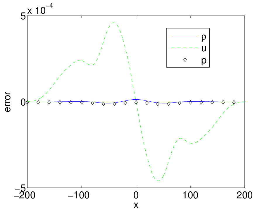
In all our numerical tests using various configurations of $\Delta t,\Delta x,\varepsilon$ we have observed $ECR\ll 1$ i.e. fast convergence. After less then $10$ iterations the convergence stops due to double precision arithmetic. This behaviour is demonstrated in Tables 1 - 9, where each table contains the errors $\lVert p_{N}-p_{N-1}\rVert$ and ECR numbers, cf. (120), for $N=k+1$ of the fixed point iteration during the first and fifth time step. The errors are computed using the discrete Sobolev norm

\lVert p\rVert_{W^{1,1}}:=\Delta x\sum\limits_{i}\left\{|p_{i}|+\left|\delta_{x}p_{i}\right|\right\}

(123)

and the discrete variant of the norm (48)

\lVert p\rVert_{S^{k}}:=\frac{1-\varepsilon^{2}}{\varepsilon}\Delta t\bigg(\Delta x\sum\limits_{i}\left(\frac{p_{i}^{2}}{\gamma-1}+\frac{(p_{k})_{i}-(p_{k})_{\infty}}{\hat{\rho}_{i}}\left(\delta_{x}p_{i}\right)^{2}\right)\bigg)^{1/2}

(124)

Here, $p_{i}$ denotes the cell average of $p$ on the $i$ -th cell, $\delta_{x}p_{i}$ is a central finite difference derivative, if the index $i$ corresponds to an inner cell, and one-sided finite difference otherwise. Tables 1-6 present the results obtained for the first and second order scheme (34) and (79), (80) for $\varepsilon=0.1$ , respectively. Furthermore, the results obtained for $\varepsilon=0.01$ are presented in Tables 7-9.

We can notice that already after one iteration the error in the discrete pressure equation is smaller then the local truncation error. Consequently, no significant differences have been observed between the numerical solution obtained by iterating the pressure once or several times, cf. Figure 1. Therefore, in the following computations we have performed just one nonlinear iteration to solve the pressure equations (102), (103), (104) numerically.

Refer to caption — Fig. 1: Two colliding acoustic pulses problem. Numerical solution for $\varepsilon=0.01$ obtained by the second order scheme without any limiters, $\hat{\nu}=0.9$ , $\nu=90$ , ${\color[rgb]{0,0,0}c_{\mathbf{stab}}}=1/12$ . The dashed lines represent the solution with $20$ iterations and the straight lines show the solution without iterations. Top left: density. Top right: velocity. Bottom left: pressure. Bottom right: difference between density, velocity and pressure.

	1st time step		5th time step
$N$	$W^{1,1}$ -error	ECR	$W^{1,1}$ -error	ECR
1	3.60e-04	1.000	7.91e-04	1.000
2	2.58e-06	0.007	1.32e-05	0.017
3	2.07e-08	0.008	2.47e-07	0.019
4	1.71e-10	0.008	4.88e-09	0.020
5	1.45e-12	0.009	9.83e-11	0.020
6	1.34e-13	0.092	2.12e-12	0.022
7	1.07e-13	0.799	1.55e-13	0.073
8	1.02e-13	0.955	1.48e-13	0.956
9	8.65e-14	0.848	1.48e-13	0.999
10	9.13e-14	1.055	1.32e-13	0.894
11	9.90e-14	1.084	1.31e-13	0.989
12	9.56e-14	0.966	1.31e-13	1.003
13	9.39e-14	0.982	1.40e-13	1.066

Table 1: Two colliding acoustic pulses problem.

W^{1,1}

-errors for pressure and ECR’s of the iteration (102) during the first and 5th time step using the first order scheme.

\varepsilon=0.1

\hat{\nu}=0.9

\nu_{eff}=9

	1st time step		5th time step
$N$	$S$ -error	ECR	$S$ -error	ECR
1	4.86e-05	1.000	1.92e-04	1.000
2	3.65e-07	0.008	3.68e-06	0.019
3	2.99e-09	0.008	7.37e-08	0.020
4	2.50e-11	0.008	1.49e-09	0.020
5	2.10e-13	0.008	3.05e-11	0.020
6	1.03e-14	0.049	6.23e-13	0.020
7	8.04e-15	0.784	1.69e-14	0.027
8	7.80e-15	0.970	1.29e-14	0.765
9	6.87e-15	0.881	1.38e-14	1.071
10	6.95e-15	1.011	1.13e-14	0.821
11	7.96e-15	1.145	1.05e-14	0.924
12	7.80e-15	0.980	1.09e-14	1.035
13	7.49e-15	0.961	1.23e-14	1.134

Table 2: Two colliding acoustic pulses problem.

\|\cdot\|_{S}

-errors for pressure and ECR’s of the iteration (102) during the first and 5th time step using the first order scheme.

\varepsilon=0.1

\hat{\nu}=0.9

\nu_{eff}=9

	1st time step		5th time step
$N$	$W^{1,1}$ -error	ECR	$W^{1,1}$ -error	ECR
1	8.99e-05	1.000	1.44e-04	1.000
2	3.53e-07	0.004	1.03e-06	0.007
3	1.48e-09	0.004	8.30e-09	0.008
4	6.36e-12	0.004	7.16e-11	0.009
5	8.51e-14	0.013	6.86e-13	0.010
6	6.41e-14	0.753	7.66e-14	0.112
7	6.71e-14	1.047	6.36e-14	0.830
8	5.75e-14	0.858	5.36e-14	0.843
9	5.69e-14	0.989	7.27e-14	1.358
10	6.14e-14	1.079	7.57e-14	1.040
11	5.74e-14	0.935	6.96e-14	0.920
12	5.77e-14	1.006	5.67e-14	0.814
13	7.15e-14	1.238	5.04e-14	0.890

Table 3: Two colliding acoustic pulses problem.

\|\cdot\|_{W^{1,1}}

-errors for pressure and ECR’s of the iteration (103) during the first and 5th time step using the second order scheme - first step (79).

\varepsilon=0.1

\hat{\nu}=0.9

\nu_{eff}=9

	1st time step		5th time step
$N$	$W^{1,1}$ -error	ECR	$W^{1,1}$ -error	ECR
1	2.63e-03	1.000	3.88e-03	1.000
2	1.09e-05	0.004	3.00e-05	0.008
3	4.64e-08	0.004	2.66e-07	0.009
4	2.01e-10	0.004	2.52e-09	0.009
5	9.19e-13	0.005	2.46e-11	0.010
6	1.41e-13	0.154	3.73e-13	0.015
7	1.46e-13	1.034	1.44e-13	0.387
8	1.46e-13	1.002	1.56e-13	1.079
9	1.35e-13	0.921	1.50e-13	0.963
10	1.13e-13	0.840	1.39e-13	0.930
11	1.16e-13	1.022	1.42e-13	1.018
12	1.23e-13	1.058	1.66e-13	1.173
13	1.50e-13	1.223	1.35e-13	0.811

Table 4: Two colliding acoustic pulses problem.

\|\cdot\|_{W^{1,1}}

-errors for pressure and ECR’s of the iteration (104) during the first and 5th time step using the second order scheme - 2nd step.

\varepsilon=0.1

\hat{\nu}=0.9

\nu_{eff}=9

	1st time step		5th time step
$N$	$S$ -error	ECR	$S$ -error	ECR
1	1.83e-04	1.000	4.37e-04	1.000
2	7.71e-07	0.004	4.03e-06	0.009
3	3.33e-09	0.004	3.89e-08	0.010
4	1.46e-11	0.004	3.82e-10	0.010
5	6.44e-14	0.004	3.78e-12	0.010
6	5.38e-15	0.083	3.91e-14	0.010
7	5.59e-15	1.040	5.56e-15	0.142
8	5.14e-15	0.920	5.91e-15	1.062
9	4.96e-15	0.964	5.54e-15	0.938
10	4.36e-15	0.879	4.86e-15	0.876
11	4.17e-15	0.957	5.70e-15	1.174
12	4.77e-15	1.144	6.01e-15	1.053
13	5.65e-15	1.184	5.27e-15	0.878

Table 5: Two colliding acoustic pulses problem.

\|\cdot\|_{S}

-errors for pressure and ECR’s of the iteration (104) during the first and 5th time step using the second order scheme - first step.

\varepsilon=0.1

\hat{\nu}=0.9

\nu_{eff}=9

	1st time step		5th time step
$N$	$S$ -error	ECR	$S$ -error	ECR
1	6.24e-06	1.000	1.62e-05	1.000
2	2.53e-08	0.004	1.35e-07	0.008
3	1.08e-10	0.004	1.19e-09	0.009
4	4.67e-13	0.004	1.07e-11	0.009
5	3.88e-15	0.008	9.62e-14	0.009
6	2.59e-15	0.669	2.99e-15	0.031
7	2.18e-15	0.840	2.60e-15	0.868
8	2.08e-15	0.956	2.28e-15	0.877
9	2.03e-15	0.973	2.87e-15	1.260
10	2.43e-15	1.199	2.79e-15	0.970
11	2.21e-15	0.911	2.51e-15	0.902
12	2.14e-15	0.967	2.19e-15	0.873
13	2.58e-15	1.207	2.03e-15	0.925

Table 6: Two colliding acoustic pulses problem.

\|\cdot\|_{S}

-errors for pressure and ECR’s of the iteration (104) during the first and 5th time step using the second order scheme - 2nd step.

\varepsilon=0.1

\hat{\nu}=0.9

\nu_{eff}=9

	1st time step		5th time step
$N$	$W^{1,1}$ -error	ECR	$W^{1,1}$ -error	ECR
1	1.25e-05	1.000	5.84e-06	1.000
2	8.98e-09	0.001	5.96e-09	0.001
3	1.61e-09	0.180	1.34e-09	0.224
4	1.33e-09	0.827	1.77e-09	1.327
5	1.59e-09	1.193	1.78e-09	1.002
6	1.57e-09	0.989	1.07e-09	0.601
7	1.65e-09	1.048	1.33e-09	1.243
8	1.48e-09	0.898	1.57e-09	1.180
9	1.42e-09	0.955	1.63e-09	1.041
10	1.25e-09	0.886	1.37e-09	0.839
11	1.69e-09	1.344	1.36e-09	0.995
12	1.60e-09	0.951	1.56e-09	1.143
13	1.74e-09	1.087	1.29e-09	0.831

Table 7: Two colliding acoustic pulses problem.

\|\cdot\|_{W^{1,1}}

-errors for pressure and ECR’s of the iteration (102) during the first and 5th time step using the first order scheme.

\varepsilon=0.01

\hat{\nu}=0.9

\nu_{eff}=90

	1st time step		5th time step
$N$	$S$ -error	ECR	$S$ -error	ECR
1	6.71e-06	1.000	3.71e-06	1.000
2	5.06e-09	0.001	4.15e-09	0.001
3	7.95e-10	0.157	7.23e-10	0.174
4	7.13e-10	0.898	9.90e-10	1.369
5	8.00e-10	1.121	9.48e-10	0.958
6	8.39e-10	1.048	5.74e-10	0.606
7	8.72e-10	1.040	7.35e-10	1.280
8	7.68e-10	0.881	8.62e-10	1.172
9	7.67e-10	0.998	8.78e-10	1.019
10	7.00e-10	0.913	7.70e-10	0.876
11	8.77e-10	1.253	7.56e-10	0.983
12	8.19e-10	0.934	8.37e-10	1.107
13	9.32e-10	1.137	6.92e-10	0.827

Table 8: Two colliding acoustic pulses problem.

\|\cdot\|_{S}

-errors for pressure and ECR’s of the iteration (102) during the first and 5th time step using the first order scheme.

\varepsilon=0.01

\hat{\nu}=0.9

\nu_{eff}=90

	1st time step		5th time step
$N$	$W^{1,1}$ -error	ECR	$W^{1,1}$ -error	ECR
1	7.71e-07	1.000	1.06e-06	1.000
2	9.53e-10	0.001	1.06e-09	0.001
3	8.74e-10	0.918	6.07e-10	0.575
4	9.89e-10	1.131	6.49e-10	1.068
5	8.16e-10	0.826	8.34e-10	1.286
6	9.36e-10	1.147	8.23e-10	0.987
7	1.01e-09	1.082	8.86e-10	1.076
8	9.42e-10	0.931	8.68e-10	0.981
9	9.34e-10	0.991	8.45e-10	0.973
10	8.56e-10	0.916	7.42e-10	0.879
11	8.32e-10	0.972	9.65e-10	1.299
12	8.82e-10	1.060	9.07e-10	0.940
13	8.92e-10	1.011	8.51e-10	0.939

Table 9: Two colliding acoustic pulses problem.

\|\cdot\|_{W^{1,1}}

-errors for pressure and ECR’s of the iteration (103) during the first and 5th time step using the second order scheme - first step.

\varepsilon=0.01

\hat{\nu}=0.9

\nu_{eff}=90

Experimental Convergence Rates (EOC)

In this subsection we study the experimental order of convergence (EOC). Since the exact solution is not readily available, the EOC can be computed using numerical solutions on three grids of sizes $N_{1},N_{2}:=N_{1}/2,N_{3}:=N_{2}/2$ in the following way

\mbox{EOC}:=\log_{2}\frac{\lVert u_{N_{1}}^{n}-u_{N_{2}}^{n}\rVert}{\lVert u_{N_{2}}^{n}-u_{N_{3}}^{n}\rVert}.

(125)

Here, $u_{N}^{n}$ denotes the approximate solution obtained on a mesh of $N$ cells at time $t^{n}$ . In the following, we first set $\varepsilon=0.1$ so that the problem is weakly compressible. In order to compute EOC numbers, we have successively divided the computational domain into $40,80,\ldots,1280$ cells. The final time is always set to $t=0.815$ so that the solution remains smooth. Hence, all the limiters are switched off and the slopes in the linear recovery are obtained using second order central differencing. In Tables 10-15 we present the EOC numbers obtained for the $L^{1},L^{2}$ and $L^{\infty}$ norms, respectively. The tables clearly demonstrate the first, respectively second order convergence of our schemes at $\varepsilon=0.1$ .

$N$	$L^{1}$ error	EOC	$L^{2}$ error	EOC	$L^{\infty}$ error	EOC
80	6.38e-05	1.00	1.27e-03	1.00	6.08e-02	1.00
160	1.63e-05	1.97	3.82e-04	1.74	1.92e-02	1.66
320	4.45e-06	1.87	1.74e-04	1.14	1.46e-02	0.39
640	1.22e-06	1.86	7.05e-05	1.30	7.65e-03	0.93
1280	3.36e-07	1.86	2.74e-05	1.36	4.02e-03	0.93

Table 10: Two colliding acoustic pulses problem.

L^{1},L^{2}

and

L^{\infty}

errors for density and EOC for the first order scheme (34);

\varepsilon=0.1

\hat{\nu}=0.9

\nu_{eff}=9

$N$	$L^{1}$ error	EOC	$L^{2}$ error	EOC	$L^{\infty}$ error	EOC
80	1.27e-03	1.00	1.93e-02	1.00	5.10e-01	1.00
160	3.00e-04	2.08	5.84e-03	1.72	1.72e-01	1.57
320	8.70e-05	1.79	2.59e-03	1.17	1.26e-01	0.45
640	2.14e-05	2.02	9.21e-04	1.49	6.76e-02	0.90
1280	5.25e-06	2.03	3.27e-04	1.49	3.57e-02	0.92

Table 11: Analogous results as in Table 10, but for velocity.

$N$	$L^{1}$ error	EOC	$L^{2}$ error	EOC	$L^{\infty}$ error	EOC
80	4.00e-05	1.00	5.92e-04	1.00	1.31e-02	1.00
160	1.97e-05	1.02	4.45e-04	0.41	1.68e-02	-0.35
320	5.20e-06	1.92	1.88e-04	1.25	1.30e-02	0.37
640	1.42e-06	1.87	7.96e-05	1.24	7.86e-03	0.72
1280	3.84e-07	1.88	3.14e-05	1.34	4.30e-03	0.87

Table 12: Analogous results as in Table 10, but for pressure.

$N$	$L^{1}$ error	EOC	$L^{2}$ error	EOC	$L^{\infty}$ error	EOC
80	1.12e-04	1.00	1.72e-03	1.00	3.98e-02	1.00
160	1.38e-05	3.02	3.20e-04	2.43	1.15e-02	1.79
320	2.19e-06	2.66	7.61e-05	2.07	4.32e-03	1.41
640	3.74e-07	2.55	1.88e-05	2.02	1.54e-03	1.49
1280	6.15e-08	2.60	4.64e-06	2.02	5.46e-04	1.50

Table 13: Two colliding acoustic pulses problem.

L^{1},L^{2}

and

L^{\infty}

errors for density and EOC of the second order scheme (79), (80);

\varepsilon=0.1

\hat{\nu}=0.9

\nu_{eff}=9

$N$	$L^{1}$ error	EOC	$L^{2}$ error	EOC	$L^{\infty}$ error	EOC
80	7.98e-04	1.00	1.39e-02	1.00	3.92e-01	1.00
160	1.65e-04	2.28	4.37e-03	1.67	2.06e-01	0.93
320	2.66e-05	2.63	1.03e-03	2.09	7.22e-02	1.51
640	3.99e-06	2.74	2.22e-04	2.21	2.17e-02	1.74
1280	5.97e-07	2.74	4.85e-05	2.19	6.89e-03	1.65

Table 14: Analogous results as in Table 13, but for velocity.

$N$	$L^{1}$ error	EOC	$L^{2}$ error	EOC	$L^{\infty}$ error	EOC
80	1.63e-04	1.00	2.67e-03	1.00	6.08e-02	1.00
160	1.80e-05	3.17	4.35e-04	2.62	1.58e-02	1.94
320	2.69e-06	2.74	9.54e-05	2.19	5.67e-03	1.48
640	4.67e-07	2.53	2.39e-05	2.00	2.24e-03	1.34
1280	7.68e-08	2.60	5.90e-06	2.02	8.25e-04	1.44

Table 15: Analogous results as in Table 13, but for pressure.

Next, we choose a very small value for $\varepsilon$ , $\varepsilon=0.01$ . The results are presented in Tables 16-21. Note that we can observe clearly the first and the second order experimental order of convergence of our schemes, despite a small value for $\varepsilon$ .

$N$	$L^{1}$ error	EOC	$L^{2}$ error	EOC	$L^{\infty}$ error	EOC
80	1.63e-06	1.00	2.64e-05	1.00	8.49e-04	1.00
160	2.59e-05	-3.99	5.11e-04	-4.27	1.44e-02	-4.08
320	1.42e-05	0.86	4.30e-04	0.25	2.54e-02	-0.82
640	1.05e-06	3.76	4.63e-05	3.21	5.03e-03	2.34
1280	7.41e-08	3.83	4.65e-06	3.32	4.91e-04	3.36
2560	1.67e-08	2.15	1.48e-06	1.65	2.45e-04	1.00
5120	2.86e-09	2.54	3.67e-07	2.02	8.69e-05	1.50

Table 16: Two colliding acoustic pulses problem.

L^{1},L^{2}

and

L^{\infty}

errors for deinsity and EOC of the first order scheme (34);

\varepsilon=0.01

\hat{\nu}=0.9

\nu_{eff}=90

$N$	$L^{1}$ error	EOC	$L^{2}$ error	EOC	$L^{\infty}$ error	EOC
80	9.75e-05	1.00	1.44e-03	1.00	3.10e-02	1.00
160	1.21e-03	-3.64	2.33e-02	-4.02	5.51e-01	-4.15
320	1.33e-03	-0.13	3.85e-02	-0.73	1.61e+00	-1.55
640	1.59e-04	3.06	6.46e-03	2.58	4.14e-01	1.96
1280	4.78e-05	1.74	2.78e-03	1.21	2.26e-01	0.88
2560	1.27e-05	1.91	1.05e-03	1.40	1.24e-01	0.87
5120	3.18e-06	2.00	3.70e-04	1.51	6.32e-02	0.97

Table 17: Analogous results as in Table 16, but for velocity.

$N$	$L^{1}$ error	EOC	$L^{2}$ error	EOC	$L^{\infty}$ error	EOC
80	9.44e-07	1.00	1.21e-05	1.00	2.11e-04	1.00
160	2.15e-05	-4.51	4.32e-04	-5.16	1.17e-02	-5.80
320	7.73e-06	1.47	2.26e-04	0.93	1.09e-02	0.11
640	9.84e-07	2.97	4.35e-05	2.38	3.21e-03	1.76
1280	1.00e-07	3.30	5.89e-06	2.88	6.01e-04	2.42
2560	2.46e-08	2.02	2.19e-06	1.43	3.88e-04	0.63
5120	3.85e-09	2.67	5.00e-07	2.13	1.25e-04	1.63

Table 18: Analogous results as in Table 16, but for pressure.

$N$	$L^{1}$ error	EOC	$L^{2}$ error	EOC	$L^{\infty}$ error	EOC
80	4.73e-07	1.00	7.81e-06	1.00	2.51e-04	1.00
160	8.41e-06	-4.15	2.03e-04	-4.70	9.83e-03	-5.29
320	2.60e-06	1.69	9.19e-05	1.15	6.98e-03	0.49
640	1.70e-06	0.62	7.37e-05	0.32	7.50e-03	-0.10
1280	2.46e-07	2.78	1.54e-05	2.26	2.10e-03	1.83
2560	2.23e-08	3.47	2.22e-06	2.79	4.52e-04	2.22
5120	2.65e-09	3.07	4.56e-07	2.29	1.42e-04	1.67

Table 19: Two colliding acoustic pulses problem.

L^{1},L^{2}

and

L^{\infty}

errors for density and EOC of the second order scheme (79), (80);

\varepsilon=0.01

\hat{\nu}=0.9

\nu_{eff}=90

$N$	$L^{1}$ error	EOC	$L^{2}$ error	EOC	$L^{\infty}$ error	EOC
80	1.13e-05	1.00	1.60e-04	1.00	3.39e-03	1.00
160	1.34e-03	-6.89	2.89e-02	-7.50	9.13e-01	-8.08
320	8.25e-04	0.70	2.38e-02	0.28	9.87e-01	-0.11
640	9.01e-05	3.20	3.77e-03	2.66	2.38e-01	2.05
1280	2.11e-05	2.09	1.42e-03	1.41	1.64e-01	0.54
2560	3.40e-06	2.64	3.24e-04	2.13	5.04e-02	1.70
5120	5.58e-07	2.61	7.41e-05	2.13	1.36e-02	1.89

Table 20: Analogous results as in Table 19, but for velocity.

$N$	$L^{1}$ error	EOC	$L^{2}$ error	EOC	$L^{\infty}$ error	EOC
80	3.16e-07	1.00	4.47e-06	1.00	8.40e-05	1.00
160	1.34e-05	-5.40	2.65e-04	-5.89	6.81e-03	-6.34
320	3.05e-06	2.14	9.41e-05	1.49	4.63e-03	0.56
640	2.07e-06	0.55	8.86e-05	0.09	6.86e-03	-0.57
1280	3.24e-07	2.68	2.05e-05	2.11	1.99e-03	1.78
2560	3.01e-08	3.43	2.99e-06	2.78	5.40e-04	1.88
5120	3.70e-09	3.03	6.27e-07	2.25	1.95e-04	1.47

Table 21: Analogous results as in Table 19, but for pressure.

Weakly Compressible Flow

In the third experiment we measure the efficacy of our newly developed scheme to capture weakly compressible flow features. We set $\varepsilon=1/11$ as in [19]. The computational domain is divided into $440$ equal mesh points and the CFL number is set to $\hat{\nu}=0.9$ so that $\nu_{eff}=9.9$ . The boundary conditions are periodic and the slopes in the reconstruction are computed using the minmod recovery with $\theta=2$ . The plots of the pressure obtained using the second order scheme at times $t=0.815$ and $t=1.63$ are given in Figure 2, where the initial pressure distributions are also plotted for comparison. Note that the initial data represent two pulses, where the one on the left moves to the left and the one on the right moves to the right. The data being symmetric about $x=0$ , the periodic boundary conditions act like reflecting boundary conditions. Therefore, the pulses reflect back and they superimpose at time $t=0.815$ , which produces the maximum pressure at $x=0$ . The pulses separate and move apart and at time $t=1.63$ they assume almost like the initial configuration. However, as a result of the weakly nonlinear effects, the pulses start to steepen and two shocks are about to form at $x=-18.5$ and $x=18.5$ which can be seen from the plot at $t=1.63$ .

5.1.2 Density Layering Problem

This test problem is also taken from [19] and it models the propagation of a density fluctuation superimposed in a large amplitude, short wavelength pulse. The initial data read

	$\displaystyle\rho(x,0)$	$\displaystyle=\rho_{0}+\frac{1}{2}\varepsilon\rho_{1}\left(1+\cos\left(\frac{\pi x}{L}\right)\right)+\rho_{2}\Phi(x)\sin\left(\frac{40\pi x}{L}\right),$
	$\displaystyle\rho_{0}$	$\displaystyle=1.0,\ \rho_{1}=2.0,\ \rho_{2}=0.5,$
	$\displaystyle u(x,0)$	$\displaystyle=\frac{1}{2}u_{0}\left(1+\cos\left(\frac{\pi x}{L}\right)\right),\ u_{0}=2\sqrt{\gamma},$
	$\displaystyle p(x,0)$	$\displaystyle=p_{0}+\frac{1}{2}\varepsilon p_{1}\left(1+\cos\left(\frac{\pi x}{L}\right)\right),\ p_{0}=1.0,\ p_{1}=2\gamma.$

The domain is $-L\leq x\leq L=1/\varepsilon$ with $\varepsilon=1/51$ . The function $\Phi(x)$ is defined by

\Phi(x)=\begin{cases}0,&-\frac{1}{L}\leq x\leq 0,\\ \frac{1}{2}\left(1-\cos\left(\frac{5\pi x}{L}\right)\right),&0\leq x\leq\frac{2L}{5},\\ 0,&x>\frac{2L}{5}.\end{cases}

The computation domain is divided into $1020$ equal mesh cells and the CFL number is $\hat{\nu}=0.45$ , hence $\nu_{eff}=22.95$ . The linear reconstruction is performed using the minmod limiter with $\theta=2$ and the boundary conditions are set to periodic. Note that the initial data describe a density layering of large amplitude and small wavelengths, which is driven by the motion of a right-going periodic acoustic wave with long wavelength. The main aspect of this test case is the advection of the density distribution and its nonlinear interaction with the acoustic waves. Figure 3 show the solutions obtained using the second order scheme at time $t=5.071$ and the initial distributions. Due to the high stifness, we multiplied the pressure correcture with the additional factor $1.4$ . It can be noted that up to this time the acoustic wave transport the density layer about $2.5$ units and the shape of the layer is undistorted. As in the previous problem, due to the weakly nonlinear effects, the pulse starts to steepen, leading to shock formation.

We use this test also to make a comparison of the first and second order schemes. It can be noted from Figure 3 that the second order scheme preserves the amplitude of the layer, without much damping. In order to make the comparison, in Figure 4, a zoomed portion of the layer obtained by the second order scheme and the first order scheme with the same problem parameters is plotted. In the figure the results of first order scheme is barely visible due to the excess diffusion.

5.2 Test Problems in the 2-D Case

5.2.1 Gresho Vortex Problem

In this problem we perform the simulation of the Gresho vortex [12, 21]. A rotating vortex is positioned at the centre $(0.5,0.5)$ of the computational domain $[0,1]\times[0,1]$ . The initial conditions are specified in terms of the radial distance $r=\sqrt{(x-0.5)^{2}+(y-0.5)^{2}}$ in the form

	$\displaystyle\rho(x,y,0)$	$\displaystyle=1.0,$
	$\displaystyle u(x,y,0)$	$\displaystyle=-u_{\phi}(r)\sin\phi,$
	$\displaystyle v(x,y,0)$	$\displaystyle=u_{\phi}(r)\cos\phi,$
	$\displaystyle p(x,y,0)$	$\displaystyle=\begin{cases}p_{0}+12.5r^{2},&\mbox{if}\ 0\leq r\leq 0.2,\\ p_{0}+4-4.0\log(0.2)+12.5r^{2}-20r+4\log r,&\mbox{if}\ 0.2\leq r\leq 0.4,\\ p_{0}-2+4\log 2,&\mbox{otherwise}.\end{cases}$

Here, $\tan\phi=(y-0.5)/(x-0.5)$ and the angular velocity $u_{\phi}$ is defined by

u_{\phi}(r)=\begin{cases}5r,&\mbox{if}\ 0\leq r\leq 0.2,\\ 2-5r,&\mbox{if}\ 0.2\leq r\leq 0.4,\\ 0,&\mbox{otherwise}.\end{cases}

Note that the above data is a low Mach variant of the one proposed in [21] by changing the parameter $p_{0}=\rho/(\gamma\varepsilon^{2})$ as given in [15] to obtain a low Mach number flow. In this problem we have set $\varepsilon=0.1$ .

The computational domain is divided into $80\times 80$ equal mesh cells. The boundary conditions to the left and right side are periodic. To the top and bottom sides we apply wall boundary conditions. The slopes in the recovery procedure are obtained by simple central differences without using any limiters. In order to stabilize the scheme, we increased the stabilization parameter in (98) to ${\color[rgb]{0,0,0}c_{\mathbf{stab}}}=\frac{1}{12}10^{4}$ . In Figure 5 the pseudo-colour plots of the Mach numbers are plotted which shows that very low Mach numbers of the order $0.01$ are developed in the problem. We have set the CFL number $\hat{\nu}=0.45$ and therefore, the effective CFL number is $4.5$ . In the figure we have plotted the results at times $t=1.0,2.0$ and $3.0$ so that the vortex completes one, two and three rotations completely. A comparison with the initial Mach number distribution shows that the scheme preserves the shape of the vortex very well.

5.2.2 Baroclinic Vorticity Generation Problem

The motivation for this problem is an analogous test studied in [11]. The setup contains a right-going acoustic wave, crossing a wavy density fluctuation in the vertical direction. Specifically, the initial data read

	$\displaystyle\rho(x,y,0)$	$\displaystyle=\rho_{0}+\frac{1}{2}\varepsilon\rho_{1}\left(1+\cos\left(\frac{\pi x}{L}\right)\right)+\Phi(y),\ \rho_{0}=1.0,\ \rho_{1}=0.001,$
	$\displaystyle u(x,y,0)$	$\displaystyle=\frac{1}{2}u_{0}\left(1+\cos\left(\frac{\pi x}{L}\right)\right),\ u_{0}=\sqrt{\gamma},$
	$\displaystyle v(x,y,0)$	$\displaystyle=0,$
	$\displaystyle p(x,y,0)$	$\displaystyle=p_{0}+\frac{1}{2}\varepsilon p_{1}\left(1+\cos\left(\frac{\pi x}{L}\right)\right),\ p_{0}=1.0,\ p_{1}=\gamma.$

Here, the problem domain is $-L\leq x\leq L=1/\varepsilon,0\leq y\leq L_{y}=2L/5$ with $\varepsilon=0.05$ . The function $\Phi$ is defined by

\Phi(y)=\begin{cases}\rho_{2}\frac{y}{L_{y}},&\mbox{if}\ 0\leq y\leq\frac{L_{y}}{2},\\ \rho_{2}\left(\frac{y}{L_{y}}-1\right),&\mbox{otherwise},\end{cases}

where $\rho_{2}=1.8$ .

The computational domain is divided into $400\times 80$ cells and the CFL number is $\hat{\nu}=0.45$ so that $\nu_{eff}=9$ . The boundary conditions are periodic and the slope limiting is performed with the minmod recovery with $\theta=2$ . In order to stabilize the scheme, we increased the stabilization parameter in (98) to ${\color[rgb]{0,0,0}c_{\mathbf{stab}}}=\frac{1}{12}10^{2}$ . The isolines of the density at times $t=0.0,2.0,4.0,6.0$ and $8.0$ are given in Figure 6.

Note that there are two layers in the initial density distribution and these two layers are separated by a vertical fluctuation. These layers have different accelerations from the acoustic density perturbation. Hence, a rotational motion is induced along the separating layer. As a result, the well known Kelvin-Helmholtz instability develops and long wave sinusoidal shear layers are formed. The acoustic waves continue to move and the sinusoidal shear layers will now change and become unstable at the edges because of the larger density. As a result, they create small vortex structures and grow very fast. The problem illustrates how long-wave acoustic waves produce small scale flow features.

6 Concluding Remarks

We presented a low Mach number finite volume scheme for the Euler equations of gas dynamics. The scheme is based on Klein’s non-stiff/stiff decomposition of the fluxes [19], and an explicit/implicit time discretization due to Cordier et al. [6]. Inspired by the latter, we replace the stiff energy equation by a nonlinear elliptic pressure equation. A crucial part of the method is a choice of reference pressure which ensures that both the non-stiff and the stiff subsystems are hyperbolic, and the second order PDE for the pressure is indeed elliptic. The CFL number is only related to the non-stiff characteristic speeds, independently of the Mach number.

The second order accuracy of the scheme is based on MUSCL-type reconstructions and an appropriate combination of Runge-Kutta and Crank-Nicolson time stepping strategies due to Park and Munz [26]. We have proven in Theorem 9 and 10 that our first and second order time discretizations are asymptotically consistent, uniformly with respect to $\varepsilon$ .

Since the Jacobian of the stiff flux function degenerates in the limit, as it is well-known for finite volume schemes on collocated grids in the incompressible case, we add a classical fourth order pressure derivative as stabilization [10] to the energy equation. The stabilization contains a problem-dependent parameter, which is $O(10^{-1})$ for our one-dimensional test cases, but substantially higher for the two-dimensional test cases. However, for each example, this parameter is independent of the Mach number. Given the stabilization, we can still prove asymptotic consistency for a ratio $\Delta t/\Delta x$ which is independent of the Mach number, but we have to reduce the spatial and the temporal grid sizes simultaneously as the Mach number goes to zero.

According to the results presented here, it seems to be important to study the effect of flux splittings, time discretizations, stabilization terms and their interplay upon asymptotic consistency and stability. As a step in this direction, Schütz and Noelle [24] began to study the modified equation of IMEX time discretizations of linear hyperbolic systems by Fourier analysis, identifying both stable and unstable splittings. For nonlinear problems, linearly implicit splittings such as those studied by Bispen et al. [3, 4] show very good asymptotic stability properties for the shallow water equations in one an two space-dimensions. Since these correspond to isentropic Euler equations, it is not clear how this splitting would perform for the non-isentropic gas dynamics, which we studied in the present paper.

While we have proven uniform asymptotic consistency for our time-discrete schemes in Theorem 9 and 10, an analogous theoretical result for a fully space-time discrete scheme is missing (for some recent results in this direction, see [14, 3]). Indeed, in order to obtain a stable space discretization, the stabilization term (98) had to be introduced. Consequently, our results show that also in the collocated case, for which it is well-known that it generates checkerboard instabilities in the incompressible limit, some of the AP properties can be preserved by a proper stabilization.

The results of some benchmark problems are presented in Section 5, which validate the convergence, robustness and the efficiency of the scheme to capture the weakly compressible flow features accurately.

References

[1] C. Berthon and R. Turpault. Asymptotic preserving HLL schemes. Numer. Methods Partial Differential Equations, 27(6):1396–1422, 2011.
[2] H. Bijl and P. Wesseling. A unified method for computing incompressible and compressible flows in boundary-fitted coordinates. J. Comput. Phys., 141(2):153–173, 1998.
[3] G. Bispen. Large time step IMEX finite volume schemes for singular limit flows,. PhD thesis, University of Mainz (in preparation).
[4] G. Bispen, K. R. Arun, M. Lukáčová-Medvid’ová, and S. Noelle. Imex large time step finite volume methods for low froude number shallow water flows. Comm. Comput. Phys., 16:307–347, 2014.
[5] A. J. Chorin. The numerical solution of the Navier-Stokes equations for an incompressible fluid. Bull. Amer. Math. Soc., 73:928–931, 1967.
[6] F. Cordier, P. Degond, and A. Kumbaro. An asymptotic-preserving all-speed scheme for the Euler and Navier-Stokes equations. J. Comput. Phys., 231(17):5685–5704, 2012.
[7] T. A. Davis. Algorithm 832: UMFPACK V4.3—an unsymmetric-pattern multifrontal method. ACM Trans. Math. Software, 30(2):196–199, 2004.
[8] P. Degond and M. Tang. All speed scheme for the low Mach number limit of the isentropic Euler equations. Commun. Comput. Phys., 10(1):1–31, 2011.
[9] S. Dellacherie. Analysis of Godunov type schemes applied to the compressible Euler system at low Mach number. J. Comput. Phys., 229(4):978–1016, 2010.
[10] J. Ferziger and M. Peric. Computational Methods for Fluid Dynamics, 3rd rev. ed. Springer-Verlag, Berlin Heidelberg New York, 2002.
[11] K. J. Geratz. Erweiterung eines Godunov-Typ-Verfahrens für mehrdimensionale kompressible Strömungen auf die Fälle kleiner und verschwindender Machzahl. PhD thesis, RWTH Aachen, Aachen, Germany, 1998.
[12] P. M. Gresho and S. T. Chan. On the theory of semi-implicit projection methods for viscous incompressible flow and its implementation via a finite element method that also introduces a nearly consistent mass matrix. II. Implementation. Internat. J. Numer. Methods Fluids, 11(5):621–659, 1990. Computational methods in flow analysis (Okayama, 1988).
[13] H. Guillard and C. Viozat. On the behaviour of upwind schemes in the low Mach number limit. Comput. & Fluids, 28(1):63–86, 1999.
[14] J. Haack, S. Jin, and J.-G. Liu. An all-speed asymptotic-preserving method for the isentropic Euler and Navier-Stokes equations. Commun. Comput. Phys., 12:955–980, 2012.
[15] N. Happenhofer, H. Grimm-Strele, F. Kupka, B. Löw-Baselli, and H. Muthsam. A low Mach number solver: enhancing stability and applicability. ArXiv e-prints, Dec. 2011.
[16] L. B. Hoffmann. Ein zeitlich selbstadaptives numerisches Verfahren zur Berechnung von Strömungen aller Mach-Zahlen basierend auf Mehrskalenasymptotik und diskreter Datenanalyse. PhD thesis, Universität Hamburg, Hamburg, Germany, 2000.
[17] S. Jin. Efficient asymptotic-preserving (ap) schemes for some multiscale kinetic equations. SIAM J. Sci. Comput., 21(2):441–454, 1999.
[18] S. Klainerman and A. Majda. Singular limits of quasilinear hyperbolic systems with large parameters and the incompressible limit of compressible fluids. Comm. Pure Appl. Math., 34(4):481–524, 1981.
[19] R. Klein. Semi-implicit extension of a Godunov-type scheme based on low Mach number asymptotics. I. One-dimensional flow. J. Comput. Phys., 121(2):213–237, 1995.
[20] R. Klein, N. Botta, T. Schneider, C. D. Munz, S. Roller, A. Meister, L. Hoffmann, and T. Sonar. Asymptotic adaptive methods for multi-scale problems in fluid mechanics. J. Engrg. Math., 39(1-4):261–343, 2001. Special issue on practical asymptotics.
[21] R. Liska and B. Wendroff. Comparison of several difference schemes on 1D and 2D test problems for the Euler equations. SIAM J. Sci. Comput., 25(3):995–1017 (electronic), 2003.
[22] A. Meister. Asymptotic single and multiple scale expansions in the low Mach number limit. SIAM J. Appl. Math., 60(1):256–271 (electronic), 2000.
[23] C.-D. Munz, S. Roller, R. Klein, and K. J. Geratz. The extension of incompressible flow solvers to the weakly compressible regime. Comput. & Fluids, 32(2):173–196, 2003.
[24] S. Noelle and J. Schütz. Flux splitting: A notion on stability. Technical Report 382, IGPM, RWTH Aachen University, Germany (2014). Submitted to J. Sci. Comput..
[25] L. Pareschi and G. Russo. Implicit-Explicit Runge-Kutta schemes and applications to hyperbolic systems with relaxation. J. Sci. Comput., 25(1-2):129–155, 2005.
[26] J. H. Park and C.-D. Munz. Multiple pressure variables methods for fluid flow at all Mach numbers. Internat. J. Numer. Methods Fluids, 49(8):905–931, 2005.
[27] E. Turkel. Preconditioned methods for solving the incompressible and low speed compressible equations. J. Comput. Phys., 72(2):277–298, 1987.

		$\displaystyle\quad(\rho E)^{n+1}-\widehat{\rho E}$
		$\displaystyle=\frac{p^{n+1}-\widehat{p}}{\gamma-1}+\frac{\varepsilon^{2}\widehat{\rho}}{2}\left(\\|\mathbf{u}^{n+1}\\|^{2}-\\|\widehat{\mathbf{u}}\\|^{2}\right)$
		$\displaystyle=\frac{p^{n+1}-\widehat{p}}{\gamma-1}+\frac{\varepsilon^{2}\widehat{\rho}}{2}\left(-2\frac{1-\varepsilon^{2}}{\varepsilon^{2}}\,\frac{\Delta t}{\widehat{\rho}}\,\widehat{\mathbf{u}}\cdot\nabla p^{n+1}+\frac{(1-\varepsilon^{2})^{2}}{\varepsilon^{4}}\,\frac{\Delta t^{2}}{\widehat{\rho}^{2}}\,\\|\nabla p^{n+1}\\|^{2}\right)$
		$\displaystyle=\frac{p^{n+1}-\widehat{p}}{\gamma-1}-(1-\varepsilon^{2})\,\Delta t\,\widehat{\mathbf{u}}\cdot\nabla p^{n+1}+\frac{(1-\varepsilon^{2})^{2}}{2\varepsilon^{2}}\,\frac{\Delta t^{2}}{\widehat{\rho}}\,\\|\nabla p^{n+1}\\|^{2}$		(45)