Finite temperature free fermions and the Kardar-Parisi-Zhang equation at finite time
Abstract
We consider the system of one-dimensional free fermions confined by a harmonic well at finite inverse temperature . The average density of fermions at position is derived. For and , is given by a scaling function interpolating between a Gaussian at high temperature, for , and the Wigner semi-circle law at low temperature, for . In the latter regime, we unveil a scaling limit, for , where the fluctuations close to the edge of the support, at , are described by a limiting kernel that depends continuously on and is a generalization of the Airy kernel, found in the Gaussian Unitary Ensemble of random matrices. Remarkably, exactly the same kernel arises in the exact solution of the Kardar-Parisi-Zhang (KPZ) equation in 1+1 dimensions at finite time , with the correspondence .
There is currently intense activity in the field of low dimensional quantum systems. This is motivated by new experimental developments for manipulating fundamental quantum systems, notably ultra-cold atoms [1, 2], where the confining potentials are optically generated. One of the most fundamental quantum systems is that of non-interacting spinless fermions in one dimension, confined in a harmonic trap . Recently, the zero temperature () properties of this system have been extensively studied [2, 3, 4, 5, 6, 7, 8, 9], and a deep connection between this free fermion problem and random matrix theory (RMT) has been established. Specifically, the probability density function (PDF) of the positions ’s of the fermions, given by the modulus squared of the ground state wave function , can be written as
| (1) |
with , and where is a normalization constant. Eq. (1) shows that the rescaled positions ’s behave statistically as the eigenvalues of random matrices of the Gaussian Unitary Ensemble (GUE) of random matrix theory (RMT) [10, 11].
In particular, the average density of free fermions in the ground state is given, in the large limit, by the Wigner semi-circle law [10, 11],
| (2) |
where , on the finite support . An important property of free fermions at , inherited from their connection with the eigenvalues of random matrices (1), is that they constitute a determinantal point process, for any finite . This means that their statistical properties are fully encoded in a two-point kernel from which any -point correlation function can be written as a determinant built from [see Eqs. (24, 25) below].
Early developments in RMT focused on the bulk regime, where both and are in the middle of the Wigner sea, say close to the origin where both and (i.e., of the order of the typical inter-particle spacing ). In this region the statistics of eigenvalues, and consequently the positions of the free fermions at (1), are described by the so called sine-kernel where . More recently, there has been a huge interest in the statistics of eigenvalues at the edge of the Wigner sea which, for fermions, corresponds to the fluctuations close to . To probe these fluctuations at the edge, a natural observable is the position of the rightmost fermion, in the ground state. From Eq. (1) we can immediately infer that the typical (quantum) fluctuations of , correctly shifted and scaled, are described by the Tracy-Widom (TW) distribution associated with the fluctuations of the largest eigenvalue of GUE random matrices [12]. Namely, one has
| (3) |
where is a random variable whose cumulative distribution can be written as a Fredholm determinant [13]
| (4) |
where is the Airy kernel [12, 14]
| (5) |
Here is the Airy function and is the projector on the interval . Remarkably, it was found [7] that for a generic confining potential of the form , the local fluctuations in the fermion problem at are universal both in the bulk and at the edge (5).
Given this beautiful connection between free fermions in a harmonic trap at and RMT (1), it is natural to study the effect of non-zero temperature in the free fermion system, for which much less is known (see however [15, 16]). Here, we analyze this system at finite and find a very rich behavior for the average density of fermions, as well as for the fluctuations of the right-most fermion. In particular, we find a fascinating link between free fermions at finite and the Kardar-Parisi-Zhang (KPZ) equation in dimensions at finite time.
Summary of results. First we compute the average density , for large . We find that there are two natural dimensionless scaling variables in this problem
| (6) |
in terms of which takes the scaling form
| (7) |
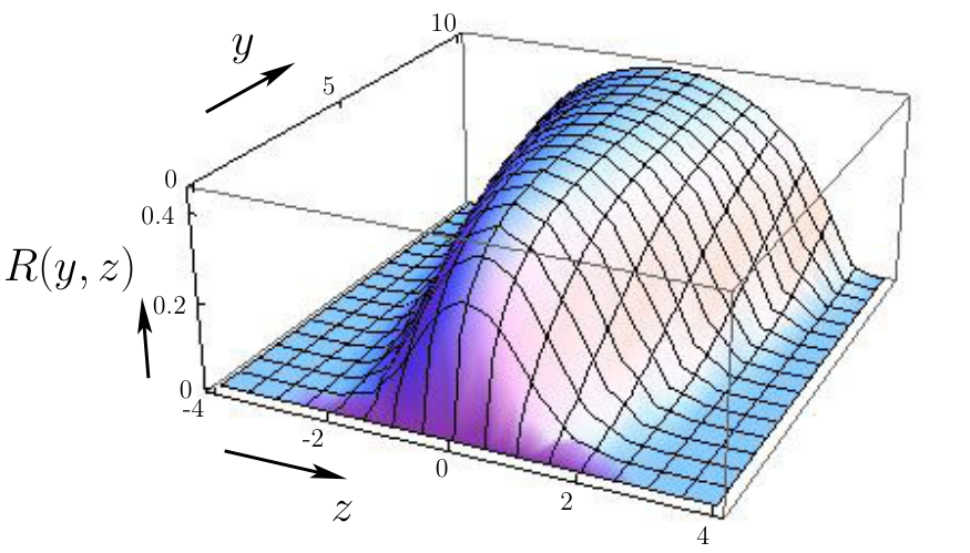
which holds in the scaling limit: (a) , but keeping fixed (i.e., ) and (b) , but keeping fixed (i.e., ). We find that the scaling function , for all and , is given by
| (8) |
where is the polylogarithm function. In Fig. 1 we show a 3d-plot of . We can check, from an asymptotic analysis of in (8), that Eq. (7) interpolates between the Wigner semi-circle (2) in the limit and the classical Gibbs-Botlzmann distribution for :
| (9) |
which holds also in the scaling limit , but keeping fixed (with the limit already taken). Note that the physical mechanism behind this interpolation is very different from those found earlier in other matrix models [17, 18].
We next consider a different low temperature scaling limit where , corresponding to the case in Eq. (7). In this scaling limit is thus given by the Wigner semicircle (2), which has a finite support . We show that for , free fermions at finite temperature in the canonical ensemble behave asymptotically as a determinantal point-process (which is not true for finite ). A similar process was studied in [19], in the context of the matrix model introduced in Ref. [15].
Close to the edge where , and for we show that this determinantal point process is characterized by a limiting kernel given by
| (10) |
which is a generalization of the Airy-kernel (5). As a consequence, we find that the cumulative distribution of the position of the rightmost fermion is given by the following Fredholm determinant [13]
| (11) |
Note that, using that in Eq. (11), we recover the TW distribution of Eq. (4) in the limit , as one should.
Remarkably, exactly the same expression as Eq. (11) was recently found in the study of the -d KPZ equation in curved geometry. The KPZ equation describes the time evolution of a height field at point and time as follows
| (12) |
where is a Gaussian white noise with zero mean and correlator . We start from the narrow wedge initial condition, , with , which gives rise to a curved (or droplet) mean profile as time evolves [20]. Defining the natural time unit and [21], the time-dependent generating function
| (13) |
of , the rescaled height at , is expressed as a Fredholm determinant [20, 22, 23, 24, 25]:
| (14) | |||
| (15) |
Comparing Eqs. (10) for the fermions and (15) for KPZ, we see that the two kernels are the same in time unit . While comparison of Eqs. (11) and (14) show that the cumulative distribution of for the free fermion problem is the same as the generating function in the KPZ equation. One can show that it interpolates between a Gumbel distribution at high (small time for KPZ) where the fermions are uncorrelated, to the Tracy-Widom distribution at (large time for KPZ).
Average density of fermions. The joint probability density function (PDF) of the positions of the fermions is constructed from the single particle wave functions
| (16) |
where is the Hermite polynomial of degree . In the canonical ensemble it is given by the Boltzmann weighted sum of slater determinants (see [26] for details)
| (17) | |||||
where is a normalization constant and where ’s are single particle energy levels (in Eq. (30) all the ’s range from to ). We first compute the mean density of free fermions , where means an average computed with (30). This amounts, up to a multiplicative constant, to integrating the joint PDF over the last variables, yielding a rather complicated expression which, however, simplifies in the large limit where the canonical ensemble and the grand-canonical ensemble become equivalent [26]. Hence, for large one obtains (see also [15, 16])
| (18) |
where is the Fermi factor and the chemical potential is fixed by imposing that mean number of fermions is :
| (19) |
We first analyze Eqs. (18) and (19) in the scaling limit where, , with and but keeping and defined in (6) fixed (implying in particular ). In this limit, the sums in (18) and (19) can be replaced by integrals and, from (19), we find . Then using the asymptotic behavior of the Hermite polynomials for large degree , one obtains [26] the scaling form in Eq. (7) together with the explicit expression of the scaling function in (8).
We then turn to Eqs. (18) and (19) in the scaling limit where , thus . Hence the average density is given by its, Wigner-semi-circle, limit (2). In this regime, an interesting scaling limit emerges close to the edges, for . To analyze the behavior of close to [30] we insert the expression of , obtained from (19), into (18) and perform a change of variable in the sum, by setting , to obtain:
| (20) |
Using the Plancherel-Rotach formula for Hermite polynomials at the edge (see for instance Ref. [31]) yields:
| (21) |
up to terms of order . Hence by inserting this asymptotic formula (21) into Eq. (20) and replacing the discrete sum over by an integral we obtain:
| (22) |
where is given by
| (23) |
and the kernel is given in (10). In the zero-temperature limit , we recover , the standard result for the mean density of eigenvalues at the edge of the spectrum of GUE random matrices [32, 14]. In Fig. 2, we show how behaves for different values of the reduced inverse temperature .
Kernel and higher order correlation functions. More generally, one can study the -point correlation function for free fermions at finite temperature. We define as
| (24) |
where is the joint PDF of the fermions at finite temperature of Eq. (30) [33]. Using the equivalence, in the large limit, between the canonical and grand-canonical ensembles, one can show that
| (25) |
where the kernel is given by
| (26) |
We first analyze the kernel (26) in the scaling limit where and keeping in (6) fixed (i.e., ). In this limit, if we are interested in the behavior of in the bulk where both and are close to the origin, one finds (see also [16, 19])
| (27) |
Note that in the low temperature limit , the Fermi factor in Eq. (27) behaves like a theta function, , implying that , which (up to a scaling factor) is the expected sine-kernel. In the inset of Fig. 3 we show a plot of the pair-correlation function for different values of the scaled inverse temperature .
However, in the low temperature scaling limit where , the kernel in the bulk is given by the sine-kernel while the interesting behavior occurs at the edge . In this limit, performing the same analysis as above (20)-(23), one finds that the kernel (26) takes the scaling form:
| (28) |
where is given in Eq. (10). In Fig. 3 we show a plot of the 2-point correlation function at the edge for different scaled inverse temperatures . The properties of determinantal point processes [34] then imply that the cumulative distribution of the position of the rightmost fermion is given by Eq. (11).
We have analyzed the effect of finite temperature on free spinless fermions in a harmonic trap in one dimension. The scaling function, showing how the average density of the system, in the bulk, crosses over from the Gaussian Gibbs-Boltzmann form at high temperatures (9) to the Wigner semi-circle law (2) at low temperatures, has been computed. For large , the equivalence between canonical and grand canonical ensembles implies that free fermion statistics can be described as a determinantal process even at finite temperature. We derived the kernel for this process at finite temperature in the bulk, and also close to the edge of the bulk at low temperature. The statistics of the rightmost fermion turns out to be governed by a finite temperature generalization of the TW distribution. The temperature dependent kernel found here also exhibit a tantalizing connection with the one appearing in exact solutions of the KPZ equation [22, 23, 24, 25] at finite times with the correspondence . This connection in fact holds for generic confining potentials such that , with , for large: the kernel is universal, and only the scalings with are modified [35]. This intriguing connection between free fermions at finite temperature and KPZ at finite time is, for the moment, a pure observation, which still lacks a deeper physical understanding. Whether it is merely an accident (holding for droplet KPZ initial conditions and in ), or the sign of a more fundamental connection will be interesting to explore in the future.
Acknowledgements.
We acknowledge stimulating discussions with P. Calabrese, T. Imamura, S. M. Nishigaki and T. Sasamoto. We acknowledge support from PSL grant ANR-10-IDEX-0001-02-PSL (PLD) ANR grant 2011-BS04-013-01 WALKMAT and in part by the Indo-French Centre for the Promotion of Advanced Research under Project 4604-3 (SM and GS) and Labex- PALM (Project Randmat) (GS).References
- [1] I. Bloch, J. Dalibard, and W. Zwerger, Rev. Mod. Phys. 80, 885 (2008).
- [2] S. Giorgini, L. P. Pitaevski, and S. Stringari, Rev. Mod. Phys. 80, 1215 (2008).
- [3] P. Calabrese, M. Mintchev, and E. Vicari, Phys. Rev. Lett. 107, 020601 (2011); J. Stat. Mech. P09028 (2011).
- [4] E. Vicari, Phys. Rev. A 85, 062104 (2012).
- [5] M. Campostrini and E. Vicari, Phys. Rev. A 82, 063636 (2010).
- [6] A. Angelone, M. Campostrini, and E. Vicari, Phys. Rev. A 89, 023635 (2014).
- [7] V. Eisler, Phys. Rev. Lett. 111, 080402 (2013).
- [8] R. Marino, S. N. Majumdar, G. Schehr, P. Vivo, Phys. Rev. Lett. 112, 254101 (2014).
- [9] P. Calabrese, P. Le Doussal, S. N. Majumdar, preprint arXiv:1411.4421.
- [10] M. L. Mehta, Random Matrices (Academic Press, Boston, 1991).
- [11] P. J. Forrester, Log-Gases and Random Matrices (London Mathematical Society monographs, 2010).
- [12] C. A. Tracy and H. Widom, Commun. Math. Phys. 159, 151 (1994).
- [13] We recall that, for a trace-class operator such that is well defined, , where . The effect of the projector in (4) is simply to restrict the integrals over to the interval .
- [14] P. J. Forrester, Nucl. Phys. B 402(3), 709 (1993).
- [15] M. Moshe, H. Neuberger, B. Shapiro, Phys. Rev. Lett. 73, 1497 (1994).
- [16] A. M. García-García, J. J. M. Verbaarschot, Phys. Rev. E 67, 046104 (2003).
- [17] R. Allez, J. -P. Bouchaud, A. Guionnet, Phys. Rev. Lett. 109, 094102 (2012).
- [18] R. Allez, J. -P. Bouchaud, S. N. Majumdar, P. Vivo, J. Phys. A: Math. Theor. 46, 015001 (2013).
- [19] K. Johansson, Probab. Theory Rel. 138, 75 (2007).
- [20] T. Imamura, T. Sasamoto, H. Spohn, J. Phys. A: Math. Theor. 46 355002 (2013).
- [21] in terms of defined in [23, 24].
- [22] T. Sasamoto, H. Spohn, Phys. Rev. Lett. 104, 230602 (2010).
- [23] P. Calabrese, P. Le Doussal, A. Rosso, Europhys. Lett. 90, 20002 (2010).
- [24] V. Dotsenko, Europhys. Lett. 90, 20003 (2010).
- [25] G. Amir, I. Corwin, J. Quastel, Comm. Pure and Appl. Math. 64, 466 (2011).
- [26] D. S. Dean, P. Le Doussal, S. N. Majumdar, G. Schehr, see supplemental material, which includes Refs [27, 28, 29].
- [27] Y. V. Fyodorov, Introduction to the Random Matrix Theory: Gaussian Unitary Ensemble and Beyond, Lond. Math. Soc. Lect. Note Ser. 322, 31 (2005).
- [28] C. Andreief, Mém. de la Soc. Sci., Bordeaux, (3) 2, 1 (1883).
- [29] J. B. Hough, M. Krishnapur, Y. Peres and B. Virág, Probability Surveys 3, 206 (2006).
- [30] The analysis at the edge is clearly identical.
- [31] P. J. Forrester, N. E. Frankel, T. M. Garoni, J. Math. Phys. 47, 023301 (2006).
- [32] M. Bowick, E. Brézin, Phys. Lett. B 268, 21 (1991).
- [33] Clearly .
- [34] See e.g. K. Johansson, Random matrices and determinantal processes, in Lecture Notes of the Les Houches Summer School 2005 (A. Bovier, F. Dunlop, A. van Enter, F. den Hollander, and J. Dalibard, eds.), Elsevier Science, (2006); arXiv:math-ph/0510038.
- [35] D. S. Dean, P. Le Doussal, S. N. Majumdar, G. Schehr, to be published.
Supplementary Material
We give the principal details of the calculations described in the manuscript of the Letter.
I Average density
The starting point of our computations is the joint probability density function (PDF) of the positions of the fermions at finite temperature . It can be expressed in terms of the single particle wave functions
| (29) |
where is the Hermite polynomial of degree and . This single particle wavefunction has an associated energy eigenvalue, where is an integer which ranges from to . From these single particle states, one can construct any generic many-body free fermion wavefunction by putting fermions in different single particle levels indexed by . The fermionic nature of the particles allows at most one particle in a given single particle level. The energy of such a many-body state is evidently, and the many-body wavefunction is just the Slater determinant . Assuming that the system is in the canonical ensemble characterized by the inverse temperature , the Boltzmann weight associated with such an excited state is simply . Hence the joint PDF of the particle positions in the canonical ensemble is given by the Boltzmann weighted sum of slater determinants
| (30) |
where is the canonical partition function of the free fermion gas
| (31) |
It is easy to check that is such that the PDF is normalized to unity.
We first compute the mean density of free fermions , where means an average computed with (30). This amounts, up to a multiplicative constant, to integrating the joint PDF over the last variables. This yields
| (32) |
To make analytic progress with these formula in Eqs. (32) and (31), it is convenient to introduce the occupation numbers which denote the number of fermions occupying the level , of energy . In terms of these occupation numbers ’s, the partition function is given by
| (33) |
where denotes the sum over all the possible occupation numbers for . In Eq. (33) if and if : this Kronecker delta function thus imposes the total number of particles to be exactly , as we are working in the canonical ensemble. Consider the density in Eq. (32). By writing out the Slater determinant explicitly, squaring it and integrating over coordinates in Eq. (32) upon using the orthonormal properties of the single particle wavefunctions, it is not difficult to show that the density in Eq. (32) can be written in terms of the ’s as
| (34) |
Note that in the limit where , the system is in the ground state characterized by if and if . Hence in this limit, Eq. (34) reads
| (35) |
as expected from the connection between free fermions at and random matrices belonging to the Gaussian Unitary Ensemble (GUE). What happens at finite temperature in the large limit? One can show (see below) that in the limit of large , one can replace the occupation numbers in Eqs. (33) and (34) by their average value such that
| (36) |
In the thermodynamic language, this amounts to use the equivalence, in the large limit, between the canonical ensemble and the grand-canonical ensemble. The average value of the occupation number is then given by the Fermi factor
| (37) |
In Eq. (37) the chemical potential is fixed by the total number of particles , according to the relation
| (38) |
We now analyze these formula (36)-(38) in the bulk (the analysis at the edge is outlined in the Letter, see Eqs. (20)-(23)).
Asymptotic analysis in the bulk
The bulk regime corresponds to the limit , and keeping fixed the following dimensionless variables
| (39) |
In this limit, the equation fixing the chemical potential (38) reads
| (40) |
This yields the relation
| (41) |
We now analyze the density given in Eqs. (36) and (37) which we evaluate for . After performing the change of variable in the sum over in (36), one obtains:
| (42) |
where we have replaced by its value given in Eq. (41) and where is given in Eq. (29). We now need an asymptotic expansion of for large (and large ). This expansion is provided by the Plancherel-Rotach formula [as given for instance in Eqs. (3.10) (3.11) of Ref. [1]]. For , one has
| (43) | |||
| (44) |
Using these formulas (43) and (44) for and – see Eq. (42) – (taking into account that , i.e., ) one finds
| (45) | |||||
| (46) |
where, in the second line, we have simply performed the change of variable . To obtain the large limit of Eq. (46) we notice that, thanks to the identity , one can replace , given in Eq. (44), in the integral over in (46) by (the remaining cosine being highly oscillating for large and thus subleading). If one finally performs the change of variable in (46), one obtains finally
| (47) |
where is the polylogarithm function. Hence from Eq. (47) one obtains the scaling form given in Eq. (7) in the Letter:
| (48) |
with
| (49) |
as given in Eq. (8) of the Letter.
To analyze the and the limits of in Eqs. (47) and (49), we need the following asymptotic behaviors of the polylogarithm function:
| (50) |
and
| (51) |
From these behaviors in (50) and (51), one finds the asymptotic behaviors of the scaling function in (49):
| (52) |
From the first line of Eq. (52), one recovers the limit where the density converges to the Gibbs-Boltzmann (Gaussian) form, given in Eq. (9) of our Letter. On the other hand, from the second line of Eq. (52), one obtains the limit of the density, which is given by the Wigner semi-circle, given in Eq. (2) of our Letter.
II Higer order correlation function and kernel
Here we focus on the -point correlation function defined as
| (53) |
where is the joint PDF of the fermions at finite temperature in Eq. (30). To compute the multidimensional integral in Eq. (53), it is useful, as in the preceding computation of , to introduce the occupation numbers . Then we note that we can rewrite the norm of any N-body eigenstate appearing in (30), of energy , and corresponding to occupied states as:
| (54) |
where and the kernel is given by
| (55) |
where is given in Eq. (29) and the are for occupied states and zero otherwise. Now one can integrate in Eq. (54), for each fixed , over the coordinates . The form of the kernel in Eq. (55) and the orthonormality of the single particle wave functions of the occupied states gaurantees that the determinantal structure in Eq. (54) survives the -fold integration. These manipulations are identical to those performed in the context of random matrix theory [2, 3, 4]. There they are most often applied to the kernel (55) built with the lowest energy eigenstates (corresponding to the ground-state wave function at ), but the same properties hold for any excited state built with single particle states. We thus obtain:
| (56) |
The averaging over the occupation numbers in Eq. (56) can be carried out by effectively passing to the grand canonical ensemble by writing (and thus rendering the ’s effectively independent Bernoulli random variables)
| (57) |
to evaluate both the numerator and the denominator of Eq. (56). Now we use the following property:
| (58) |
which holds for arbitrary averaging for which the variables are independent. It is easily seen using the (generalized) Andreief formula [5]:
| (59) |
and averaging it, using (see also [6] in the context of determinantal processes). Here we will use it for an average at fixed , i.e., and perform the integral over at the end. Using the effective independence of the in this representation, we thus obtain:
| (60) |
where
| (61) |
is the grand potential of the grand canonical ensemble. Up to this point, Eq. (60) is exact for arbitrary and . The analysis presented in the Letter is then based on the evaluation of the integrals in the denominator and numerator by the saddle point method in the limit of large , with the saddle point occurring, in our notation, at in both integrals, where is related to as , which is simply Eq. (38). This is correct as long as the corresponding quantity that is averaged does not have the form where [7]. Said otherwise, the quantity that is computed should not change the value of the chemical potential in the saddle point calculation.
Therefore, in the large limit, one obtains from (60):
| (62) |
where the kernel , obtained from (55) by replacing by its grand canonical average, i.e. its average at the saddle point in (37), is given by
| (63) |
while the chemical potential is fixed by Eq. (38). The case then yields the result for the density in Eq. (36). We remark that the quantity is referred to as the correlation density in the mathematics literature; this is because the quantity is the probability that there is a particle in each of the intervals , . Clearly such quantities exist and make sense for ensembles where the particle number varies. Indeed, note that if one formulates the problem from the start in the grand canonical ensemble, then Eq. (62) is exact as an equality. Hence the kernel exactly describes the statistics of a system in the grand canonical ensemble at the chemical potential corresponding to for all values of , and not only those corresponding to large (see also Ref. [9]).
These results in Eqs. (62) and (63) are given in the Letter in Eqs. (25) and (26). We now analyze the kernel in the bulk limit. The analysis of at the edge is outlined in the Letter.
Asymptotic limit in the bulk
We analyze the kernel in the bulk where both and are close to the center of the trap (and is of the order of the typical inter-particle distance). Hence we analyze the formula (63) and (38) , keeping in (39) fixed. In this limit the chemical potential is given by Eq. (41) and the large analysis of (63) can be performed along the same lines as we did before for the density yielding eventually Eq. (46). Indeed, using the Plancherel-Rotach asymptotic expansions (43) and (44) we obtain:
| (64) |
From the explicit expression of in Eq. (44), one obtains straighforwardly
| (65) |
And therefore the product in Eq. (64) reads, for large :
| (66) |
The second term in Eq. (66) is highly oscillating in the large limit and hence the leading contribution, once inserted in the integral over in Eq. (64), comes from the first term of Eq. (66), which is independent of . Therefore we finally obtain
| (67) |
Finally, performing the change of variable , one obtains the formula given in Eq. (27) in the Letter (see also Refs. [8, 9] for alternative derivations of this kernel).
References
- [1] P. J. Forrester, N. E. Frankel, T. M. Garoni, J. Math. Phys. 47, 023301 (2006).
- [2] M. L. Mehta, Random Matrices (Academic Press, Boston, 1991).
- [3] P. J. Forrester, Log-Gases and Random Matrices (London Mathematical Society monographs, 2010).
- [4] Y. V. Fyodorov, Introduction to the Random Matrix Theory: Gaussian Unitary Ensemble and Beyond arXiv:math-ph/0412017, Lond.Math.Soc.Lect.Note Ser.322:31-78,2005.
- [5] C. Andreief, Mém. de la Soc. Sci., Bordeaux, (3) 2, 1 (1883).
- [6] J. B. Hough, M. Krishnapur, Y. Peres and B. Virág, Probability Surveys, 3, 206 (2006).
- [7] This is clearly the case for the scaling quantities studied here.
- [8] A. M. García-García, J. J. M. Verbaarschot, Phys. Rev. E 67, 046104 (2003).
- [9] K. Johansson, Probab. Theory Rel. 138, 75 (2007).