A staggered space-time discontinuous Galerkin method for the incompressible Navier-Stokes equations on two-dimensional triangular meshes
Abstract
In this paper we propose a novel arbitrary high order accurate semi-implicit space-time discontinuous Galerkin method for the solution of the two dimensional incompressible Navier-Stokes equations on staggered unstructured triangular meshes. Isoparametric finite elements are used to take into account curved domain boundaries. The discrete pressure is defined on the primal triangular grid and the discrete velocity field is defined on an edge-based staggered dual grid. While staggered meshes are state of the art in classical finite difference approximations of the incompressible Navier-Stokes equations, their use in the context of high order DG schemes is novel and still quite rare. Formal substitution of the discrete momentum equation into the discrete continuity equation yields a sparse four-point block system for the scalar pressure, which is conveniently solved with a matrix-free GMRES algorithm. A very simple and efficient Picard iteration is then used in order to achieve high order of accuracy also in time, which is in general a non-trivial task in the context of high order discretizations for the incompressible Navier-Stokes equations. The flexibility and accuracy of high order space-time DG methods on curved unstructured meshes allows to discretize even complex physical domains with very coarse grids in both, space and time. The use of a staggered grid allows to avoid the use of Riemann solvers in several terms of the discrete equations and significantly reduces the total stencil size of the linear system that needs to be solved for the pressure. The proposed method is validated for approximation polynomials of degree up to in space and time by solving a series of typical numerical test problems and by comparing the obtained numerical results with available exact analytical solutions or other numerical reference data.
Keywords:
staggered semi-implicit space-time discontinuous Galerkin schemes , high order accuracy in space and time , staggered unstructured meshes , high order isoparametric finite elements , curved boundaries , incompressible Navier-Stokes equations1 Introduction
The discretization of the incompressible Navier-Stokes equations was mainly carried out in the past using finite difference methods [1, 2, 3, 4] as well as continuous finite element schemes [5, 6, 7, 8, 9, 10, 11]. On the contrary, the construction of high order discontinuous Galerkin (DG) finite element methods for the incompressible Navier-Stokes equations is still a very active topic of ongoing research. Obtaining high order of accuracy also in time represents an important goal in order to achieve accurate results for unsteady problems.
Several high order DG methods for the incompressible Navier-Stokes equations have been recently presented in the literature, see for example [12, 13, 14, 15, 16, 17, 18, 19], without pretending completeness. An alternative is the DG scheme proposed by Bassi et al. in [20], which is based on an extension of the technique of artificial compressibility that was originally introduced by Chorin in the finite difference context [21, 22]. Another very well known approach to discretize general convection-diffusion equations in the context of hp discontinuous Galerkin finite element methods is the one proposed by Baumann and Oden in [23, 24]. A unified analysis of several variants of the DG method applied to an elliptic model problem has been provided by Arnold et al. in [25]. We also would like to mention recent works on semi-implicit DG schemes, such as the ones presented in [26, 27, 28, 29, 30], to which our approach is indirectly related.
While the use of staggered grids is a very common practice in the finite difference community, its use is not so widespread in the development of high order DG schemes. The first staggered DG schemes, based on a vertex-based dual grid, have been proposed in [31, 32]. Other recent high order staggered DG schemes that use an edge-based dual grid have been forwarded in [33, 34, 35]. The advantage in using edge-based staggered grids is that they allow to improve significantly the sparsity pattern of the final linear system that has to be solved for the pressure.
Very recently, a staggered semi-implicit DG scheme for the solution of the two dimensional shallow water equations was presented in [35, 36] and then extended in [37] to the incompressible Navier-Stokes equations. The method presented in [37] is in principle of arbitrary high order of accuracy in space, while it reaches only second order in time. Consequently, it does not allow to recover high order accurate results for fully unsteady solutions.
In this paper we propose a new method that is based on the general ideas put forward in [35, 36, 37], but which is also able to reach high order of accuracy in time. For this purpose we construct an arbitrary high order accurate staggered space-time discontinuous Galerkin finite element scheme. By relying on staggered grids we follow the classical philosophy of staggered finite difference schemes for the incompressible Navier-Stokes equations and for the free surface shallow water and Navier-Stokes equations, see [1, 2, 3, 4, 38, 39, 40, 41, 42, 43, 44]. In the context of staggered finite difference schemes we also would like to mention the so-called multiple pressure variables approach (MPV) [45, 46, 47], which is based on the asymptotic analysis of the compressible Navier-Stokes equations and is able to preserve also their incompressible limit.
Our staggered semi-implicit space-time DG method proposed in this paper can be seen as a natural extension of the staggered semi-implicit DG scheme proposed in [37] to arbitrary high order of accuracy also in time. However, we emphasize that this extension is not straightforward for the complete convective-viscous problem. In the staggered DG scheme presented in [37], the discrete pressure is defined on the control volumes of the primal triangular mesh, while the discrete velocity vector field is defined on an edge-based, quadrilateral dual mesh. In the proposed staggered space-time DG scheme, the spatial control volumes are simply extended to the corresponding space-time control volumes by using the tensor product of the spatial control volume with the time interval of each time step, hence leading to triangular base prisms for the primal mesh and to quadrilateral base prisms for the dual mesh.
The nonlinear convective terms are discretized explicitly by using a standard DG scheme [48, 49, 50] based on the local Lax-Friedrichs (Rusanov) flux [51], while the viscous terms are discretized implicitly using a fractional step method 11 1 Note that high order in time is obtained later by a Picard iteration, which embraces the entire scheme in each time step.. The DG discretization of the viscous fluxes is based on the formulation of Gassner et al. [52], who obtained the viscous numerical flux from the solution of the Generalized Riemann Problem (GRP) of the diffusion equation.
The discrete momentum equation is then inserted into the discrete continuity equation in order to obtain the discrete form of the pressure Poisson equation. The chosen dual grid used here is taken as the one used in [53, 54, 55, 34, 36], which leads to a sparse four-point block system for the scalar pressure. Once the new pressure field is known, the velocity vector field can subsequently be updated directly. A Picard iteration procedure that embraces the entire scheme in each time step is then used in order to achieve arbitrary high-order of accuracy also in time for the nonlinear convective term, without introducing a non linearity in the system for the pressure.
2 DG scheme for the 2D incompressible Navier-Stokes equations
2.1 Governing equations
The two dimensional incompressible Navier-Stokes equations are given by
| (1) | |||||
| (2) |
where indicates the normalized fluid pressure; is the physical pressure and is the constant fluid density; is the kinematic viscosity coefficient; is the velocity vector; and are the velocity components in the and direction, respectively; is a (nonlinear) algebraic source term; is the flux tensor of the nonlinear convective terms, namely:
2.2 Staggered unstructured grid
Through this paper we use the same unstructured staggered grid in space as the one used in [37, 36]. In the following, we briefly summarize the grid construction and the main notation for the spatial grid. After that, the primary and dual spatial elements are extended to the primary and dual space-time control volumes, respectively.
2.2.1 Unstructured staggered grid in space
The spatial computational domain is covered with a set of non-overlapping triangles with . By denoting with the total number of edges, the physical th edge will be called . denotes the set of indices corresponding to boundary edges. The three edges of each triangle constitute the set defined by . For every there exist two triangles and that share . We assign arbitrarily a left and a right triangle called and , respectively. The standard positive direction is assumed to be from left to right. Let denote the unit normal vector defined on the edge and oriented with respect to the positive direction from left to right. For every triangular element and edge , the neighbor triangle of element that share the edge is denoted by .
For every the quadrilateral element associated to is called and it is defined, in general, by the two centers of gravity of and and the two terminal nodes of , see also [53, 55, 36]. We denote by the intersection element for every and . Figure 1 summarizes the used notation, the primal triangular mesh and the dual quadrilateral grid.
According to [37], we will call the mesh of triangular elements the main grid or primal grid and the quadrilateral grid is termed the dual grid.
The dual grid is covering with non-overlapping quadrilaterals, so we define the equivalent quantities given for the main grid also to the dual one, briefly: is the total amount of edges of ; indicates the physical -th edge; , the set of edges of is indicated with ; , and are the left and the right quadrilateral element, respectively; is the standard normal vector defined on and assumed positive with respect to the standard orientation on (defined, as for the main grid, from the left to the right). Finally, each triangle is defined starting from an arbitrary node and oriented in counter-clockwise direction. Similarly, each quadrilateral element is defined starting from the point and oriented in counter-clockwise direction.
2.2.2 Space-time extension
In the time direction we cover the time interval with a sequence of times . We denote the time step by and the corresponding time interval by for . In order to ease notation, sometimes we will use the abbreviation . In this way the generic space-time element defined in the time interval is given by for the main grid and for the dual grid.
Figure 2 shows a graphical representation of the primary and dual space-time control volumes.
2.3 Space-time basis functions
According to [36, 37] we proceed as follows: we first construct the polynomial basis up to a generic polynomial degree on some triangular and quadrilateral reference elements. In order to do this we take as the reference triangle and the unit square as the reference quadrilateral element . Using the standard nodal approach of conforming continuous finite elements, we obtain basis functions on and basis functions on . The connection between reference and physical space is performed by the maps for every ; for every and its inverse, called and , respectively. The maps from the physical coordinates to the reference one can be constructed following a classical sub-parametric or a complete iso-parametric approach. In the same way we construct the time basis functions on a reference interval for polynomials of degree . In this case the resulting basis functions are defined as the Lagrange interpolation polynomials passing through the Gauss-Legendre quadrature points for the unit interval. For every time interval , the map between the reference interval and the physical one is simply given by for every . Using the tensor product we can finally construct the basis functions on the space-time elements and such as and . The total number of basis functions becomes and . By introducing two sorting functions and , defined as
| (4) |
we can explicit the form of and for and in terms of space and time basis functions:
Remark how can be seen as a temporal layer selector function, so all the indexes such that represent the spatial degrees of freedom (DoF) at the time layer , for every fixed . In the same way represents the time evolution of the DoF inside the space-time element . An example of how the sorting functions act is shown in Figure 3.
2.4 Semi-implicit space-time DG scheme
The discrete pressure is defined on the main grid, namely , while the discrete velocity vector field is defined on the dual grid, namely .
The numerical solution of - is represented inside the space-time control volumes of the primal and the dual grid during the current time interval by piecewise space-time polynomials as follows:
| (5) |
| (6) |
where the vectors of basis functions and are generated via the mappings from on and on , respectively.
A weak formulation of the continuity equation is obtained by multiplying it by and integrating over a control volume , for every . The resulting weak formulation reads
| (7) |
Similarly, multiplication of the momentum equation by and integrating over a control volume yields
| (8) |
for every and . Using integration by parts Eq. becomes
| (9) |
where indicates the outward pointing unit normal vector. Due to the discontinuity of and at element boundaries, equations and have to be split. Note, however, that thanks to the use of a staggered grid we do not need a Riemann solver here, since all the quantities are readily defined where needed for the flux computation. In other words, the velocity is continuous across the boundaries of the triangles on the main grid and the pressure is continuous across the boundaries of the dual quadrilateral grid.
| (10) |
and
| (11) |
where ; ; and . Using definitions and , we conveniently rewrite the above equations as
| (12) |
and
| (13) |
where we have used the standard summation convention for the repeated index . Integrating the first integral in by parts in time we obtain
| (14) |
In Eq. we can recognize the fluxes between the current space-time element , the future space-time slab and the past space-time elements, as well as an internal space-time volume contribution that connects the layers inside the space-time element in an asymmetric way. Note how the asymmetry affects only the space-time volume contribution in . This is due to the nature of the the time derivative operator, which has a natural positive direction given by the causality principle in time. By substituting Eq. into we obtain the following weak formulation of the momentum equation in space-time:
| (15) |
For every and , Eqs. - are written in a compact matrix form as
| (16) |
and
| (17) |
respectively, where:
| (18) | |||||
| (19) | |||||
| (20) | |||||
| (21) |
| (22) |
| (23) |
| (24) |
| (25) |
Remark how introduces, for polynomial degrees , an asymmetric contribution in time. The action of matrices and can be generalized by introducing a new matrix , defined as
| (26) |
where is a sign function defined by
| (27) |
In this way and , and then Eq. becomes in terms of
| (28) |
or, equivalently,
| (29) |
In order to further ease notation, we will use the abbreviation henceforth and will write Eqs. - as follows:
| (30) | |||
| (31) |
where is an appropriate discretization of the nonlinear convective, viscous and source terms. The details for the computation of will be presented later. Formal substitution of the discrete momentum equation into the discrete continuity equation , see also [39, 35, 36, 37], yields
| (32) |
We have now to choose a time discretization for the nonlinear convective-viscous term. The simplest choice would be to take explicitly, so in this case becomes a known term at time and hence Eq. would represent a four-point block system for the new pressure , as proposed in [37]. Unfortunately, in problems when the convective-viscous effects cannot be neglected, this will produce only a low order accurate method in time. The problem in this case is that the convective-viscous contribution in the time interval is based on the old information and does not see the effects of the new pressure in the time interval . Furthermore, if we take implicitly, then system becomes nonlinear and it would be very cumbersome to solve it. In order to overcome this problem we introduce a simple Picard iteration to introduce the information of the new pressure into the viscous and convective terms, but without introducing a nonlinearity in the final system to be solved. This approach is inspired by the local space-time Galerkin predictor method proposed for the high order time discretization of schemes in [57, 56]. Hence, for , we rewrite system as
| (33) |
or, by introducing the boundary elements (see e.g. [37]),
| (34) |
where and are the natural extension of and on triangular dual boundary elements, see e.g. [37]. Now the right hand side of Eq. can be computed by using the velocity field at the old Picard iteration and including the viscous effects using a fractional step type procedure. In this way, Eq. represents a block four-point system for the new pressure . Once the new pressure field is known, the velocity vector field at the new Picard iteration can be readily updated from the momentum equation .
2.5 Nonlinear convection-diffusion
To close the problem it remains to specify how to construct the nonlinear convection-diffusion operator . Following the ideas of [37], a space-time DG scheme for the convection-diffusion terms on the dual mesh is given by
| (35) |
and the numerical flux for both, the convective and the viscous contribution, is given such as in [51, 52, 56], and reads
| (36) |
with
| (37) |
which contains the maximum eigenvalue of the Jacobian matrix of the purely convective transport operator in normal direction, see [35], and the stabilization term for the viscous flux, see [56, 52]. Furthermore, the and denote the velocity vectors and their gradients, extrapolated to the boundary of from within the element and from the neighbor element, respectively. and are the maximum radii of the inscribed circle in and the neighbor element, respectively. We discretize the velocity explicitly but its gradient has to be taken implicitly, in order to avoid additional restrictions on the maximum time step given by the viscous terms. In viscosity dominated problems, this allows us to use both, high viscosity and large time steps. After integration of the first term of (35) by parts in time the resulting fully discrete formulation of becomes
| (38) |
where
| (39) | |||||
Due to the explicit treatment of the nonlinear convective terms, the above method requires that the time step size is restricted by a CFL-type restriction for DG schemes, namely:
| (40) |
where is the smallest incircle diameter; ; and is the maximum convective speed. Furthermore, the time step of the global semi-implicit scheme is not affected by the local time step used for the time integration of the convective terms if a local time stepping / subcycling approach is employed, see [58, 59]. Implicit discretization of the viscous contribution in involves two five-point block systems (one for each velocity component) that can be efficiently solved using a matrix-free GMRES algorithm [60]. The solution of this system is not necessary in problems where the viscous term is small enough to be integrated explicitly in time. In that case, i.e. for explicit discretizations of the viscous terms, one has to include the additional explicit time step restriction for parabolic PDE in eq. .
Once has been computed, we set . As initial guess we can take the old velocity , or the extrapolation of into the interval .
2.6 Pressure correction formulation and final algorithm
The preliminary algorithm described above, as formulated by Eqs. , , still contains an important drawback: indeed, Eq. does not depend on the pressure of the previous Picard iteration and hence the algorithm does not see the effect of the pressure in the time interval . In order to overcome the problem we introduce the contribution of the pressure from the previous Picard iteration directly into Eq. . Then, we update the velocity with the new pressure . With this modification, Eqs. , , and hence the final algorithm become:
| (41) |
| (42) |
As initial guess for the pressure one can take , but one could also choose the extrapolation of into . One time step of the final algorithm can be summarized as follows:
- 1.
Initialize and using the known information from ;
- 2.
Picard iteration over :
- (a)
compute using , i.e. convective terms are discretized explicitly and viscous terms implicitly; then set ,
- (b)
compute by solving the discrete pressure Poisson equation ,
- (c)
update explicitly from ;
- (a)
- 3.
set and .
For the spatial computational domain we can apply the remark given in [37] and so either use a subparametric or a complete isoparametric representation. The second approach requires to store more information about each element, but it also allows to generalize the shape of the elements. This property is crucial when we try to discretize complex curved domains with a very coarse grid. In any case, this generalization does not affect the computational time during run-time, since it interests only the construction of the geometry-dependent matrices in the preprocessing stage of the algorithm.
2.7 Splitting of the space-time matrices into a spatial and temporal part
Even if the shape of the main matrices is similar compared to the ones introduced in [37], the number of degree of freedom and the integral values are, in general, different. Due to the tensor product construction of the space-time basis functions, we can split the main integrals - and into a spatial and a temporal part. Briefly, the space-time matrices are generated from the spatial matrices of [37], componentwise, as:
| (44) | |||||
| (45) | |||||
| (46) | |||||
| (47) | |||||
| (48) |
where the apex means that the matrix is the one constructed in [37]; and are two time matrices defined as
| (49) | |||||
| (50) |
Remark how the action of the matrix defined in is symmetric only if .
3 Numerical test problems
In this section we study the accuracy of our new numerical method by solving some classical numerical benchmark problems, such as the lid-driven cavity flow, the unsteady oscillatory flow in a pipe or the unsteady flow past a circular cylinder. In particular, we perform quantitative comparisons between the numerical solution and available exact analytical solutions wherever possible.
3.1 Convergence test using a manufactured solution
In order to study the accuracy of the proposed space-time DG method, we need an exact unsteady solution of -. For that purpose, we propose a so-called manufactured solution in this section, which also makes use of a linear source term of the type . The exact analytical solution for the velocity and the pressure is constructed so that
| (51) |
with the amplitudes and . Using the manufactured solution we can compute all terms in exactly and hence obtain a source term that balances the momentum equation. Remark that the velocity field must be divergence-free (), hence . In the present test case, we take ; ; ; ; ; according to condition ; and . The temporal accuracy is chosen equal to the spatial one, the total number of Picard iterations is taken as and for the present test. The computational domain is ; the exact velocity field and pressure are taken as initial conditions and the exact pressure is also specified on as boundary condition. The error between the analytical and the numerical solution is computed as
where the subscript refers to the numerical solution obtained at the final time . The resulting rate of convergence is shown in Table . We observe that the optimal order of convergence is obtained up to for the present unsteady test.
| 40 | 1.217E-01 | 9.572E-02 | - | - | 8.740E-03 | 1.052E-02 | - | - |
|---|---|---|---|---|---|---|---|---|
| 160 | 2.678E-02 | 2.362E-02 | 2.2 | 2.0 | 8.833E-04 | 1.065E-03 | 3.3 | 3.3 |
| 640 | 6.050E-03 | 5.527E-03 | 2.1 | 2.1 | 1.050E-04 | 9.103E-05 | 3.1 | 3.5 |
| 2560 | 1.758E-03 | 1.497E-03 | 1.8 | 1.9 | 1.347E-05 | 7.820E-06 | 3.0 | 3.5 |
| 40 | 7.703E-04 | 1.425E-03 | - | - | 5.315E-05 | 7.135E-05 | - | - |
| 160 | 3.864E-05 | 4.999E-05 | 4.3 | 4.8 | 1.143E-06 | 1.418E-06 | 5.5 | 5.7 |
| 640 | 2.425E-06 | 1.974E-06 | 4.0 | 4.7 | 3.102E-08 | 2.945E-08 | 5.2 | 5.6 |
3.2 The Womersley problem
Here we consider an unsteady, viscosity-dominated test problem for which the incompressible Navier-Stokes equations have a nontrivial exact solution, namely the fluid flow inside a rigid planar pipe that is driven by a sinusoidal pressure gradient of the type
| (52) |
In this test denotes the tube length; is the amplitude of the pressure oscillation; is the density of the fluid; is the frequency of the oscillation; and indicate the inlet and the outlet pressure, respectively; is the real part operator. By imposing Eq. at the tube ends, the exact analytical solution for the three dimensional, axially symmetric case was found by Womersley in [61]. It can be derived also for the two dimensional planar case. The resulting axial velocity is uniform in the direction and is given by
| (53) |
where ; ; ; and is the value of the bottom.
For the present test ; and . We take a set of successively refined grids in order to show the convergence behaviour to the exact solution with respect to the order in space and in time. According to [61] the nonlinear convection effect is neglected for the present test. Thus, the stability of our scheme is not restricted by the CFL condition on the fluid velocity. Since we use very large time steps and a high viscosity coefficient in this test, the implicit treatment of the viscous terms is necessary to allow large time steps. In particular we choose and . On the coarsest grid we use , then the time step is reduced proportional to the spatial grid size. No-slip boundary conditions are imposed on the top and the bottom boundary, while the pressure is imposed at the inlet and the outlet boundary on the left and on the right, respectively. The number of Picard iterations is given by for all simulations.


| 1 | 1 | 46 | 6 | 5.7880182E-02 | 1.8848423E-03 | - | - |
|---|---|---|---|---|---|---|---|
| 1 | 1 | 184 | 12 | 1.7635947E-02 | 5.5901107E-04 | 1.7 | 1.8 |
| 1 | 1 | 736 | 24 | 4.6206559E-03 | 1.4587701E-04 | 1.9 | 1.9 |
| 1 | 1 | 2944 | 48 | 1.1683966E-03 | 3.7404869E-05 | 2.0 | 2.0 |
| 2 | 2 | 46 | 6 | 7.0716231E-03 | 2.6412698E-04 | - | - |
| 2 | 2 | 184 | 12 | 4.8160864E-04 | 3.8846170E-05 | 3.9 | 2.8 |
| 2 | 2 | 736 | 24 | 3.0677533E-05 | 7.2036760E-06 | 4.0 | 2.4 |
| 2 | 2 | 2944 | 48 | 1.9295385E-06 | 1.6070616E-06 | 4.0 | 2.2 |
| 3 | 3 | 46 | 6 | 9.8372146E-04 | 1.2793693E-05 | - | - |
| 3 | 3 | 184 | 12 | 7.7144497E-05 | 7.8462176E-07 | 3.7 | 4.0 |
| 3 | 3 | 736 | 24 | 5.0814347E-06 | 4.8795894E-08 | 3.9 | 4.0 |
| 3 | 3 | 2944 | 48 | 3.2173776E-07 | 3.0326872E-09 | 4.0 | 4.0 |
| 4 | 4 | 46 | 6 | 7.3692980E-05 | 5.1193160E-07 | - | - |
| 4 | 4 | 184 | 12 | 1.2539784E-06 | 2.1649081E-08 | 5.9 | 4.6 |
| 4 | 4 | 736 | 24 | 2.1930727E-08 | 1.1576584E-09 | 5.8 | 4.2 |
| 4 | 4 | 2944 | 48 | 1.0258845E-09 | 7.0131498E-11 | 4.4 | 4.0 |
The resulting convergence results, using the norm as in the previous example, are shown in Table 2. Observe how a non-optimal order of convergence is achieved for the velocity for odd order schemes, while the optimal convergence rate is achieved for the pressure for all polynomial degrees. Note that when using the semi-implicit staggered DG method introduced in [36] only a second order of convergence could be achieved for this unsteady test problem, while full high order convergence in space and time is obtained with the new scheme presented in this paper. In Figure 4 we show the time series of the axial velocity and the pressure in a given point for the coarsest grid configuration . While piecewise linear space-time polynomials are not able to reproduce the sinusoidal signal well with only six time steps, the piecewise quadratic and higher order approximations in space and time yield an almost perfect match with the exact solution even on this extremely coarse space-time grid.
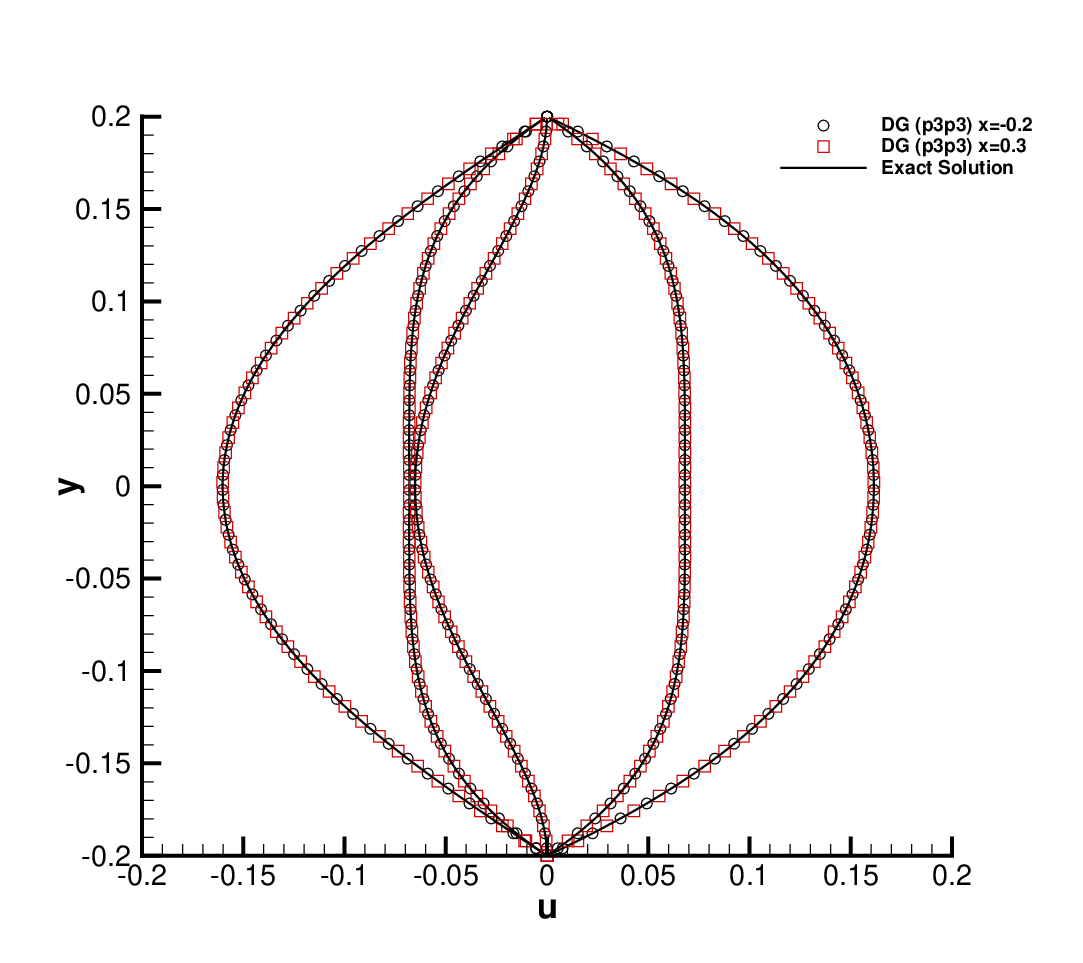
In Figure 5 we compare the resulting numerical velocity profiles against the exact solution at several times for the case and . Two different locations, and , are plotted in order to show that the profile is constant in the -direction. One observes that there is no visible difference between numerical and exact solution in Fig. 5.
3.3 Taylor-Green vortex
Another widely used testcase for the verification of numerical methods for the incompressible Navier-Stokes equations is the Taylor-Green vortex problem. The analytical unsteady solution is given by
| (54) | |||||
| (55) | |||||
| (56) |
The computational domain is and is extended using periodic boundary conditions on all the boundaries.

As implied by Eqs. -, the resulting velocity field initially appears as depicted in Figure 6 and then starts to lose energy according to the friction effects. For the present test we consider several grid refinements; ; ; and is chosen according to the CFL time restriction for the nonlinear convective terms. The numerical convergence results are shown in Table 3. We find that the optimal convergence rates are achieved for this important nontrivial test problem with periodic boundary conditions.
| 40 | 3.088E-01 | – | 5.588E-02 | – | 5.895E-03 | – | 1.669E-03 | – |
|---|---|---|---|---|---|---|---|---|
| 160 | 8.868E-02 | 1.8 | 5.765E-03 | 3.3 | 4.730E-04 | 3.6 | 3.109E-05 | 5.7 |
| 640 | 2.267E-02 | 2.0 | 7.052E-04 | 3.0 | 2.387E-05 | 4.3 | 6.233E-07 | 5.6 |
| 2560 | 5.476E-03 | 2.0 | 8.452E-05 | 3.1 | 1.312E-06 | 4.2 | 1.297E-08 | 5.6 |
3.4 Double shear layer
The numerical scheme is applied here to a test case studied in [62], which contains a high initial velocity gradient. We take and, as initial condition, we consider a perturbed double shear layer profile:
| (60) | |||||
| (61) |
where and are the normalized vertical and horizontal coordinates, respectively; is a parameter that determines the slope of the shear layer; and is the amplitude of the initial perturbation. For the present test we set ; ; ; and . The time step is chosen according to the CFL condition for the nonlinear convective terms and four Picard iterations have been used in this simulation. The domain is covered with a total number of only triangles and periodic boundary conditions are imposed everywhere. The resulting vorticity pattern is reported at several times in Figure 7.


The two thin shear layers evolve into several vortices, as observed in [62], and overall the small flow structures seem to be relatively well resolved also at the final time , even if a very coarse grid has been used in space and time.
3.5 Lid-driven cavity flow
We consider here another classical benchmark problem for the incompressible Navier-Stokes equations, namely the lid-driven cavity problem [63]. This test case is solved numerically with the new staggered space-time DG scheme on very coarse grids using polynomial degrees of and in space and time, respectively. Let , set velocity boundary conditions and on the top boundary (i.e. at ) and impose so-slip wall boundary conditions on the other edges. As initial condition we take . We use a grid with only triangles for and triangles for .
For the present test is taken according to the CFL condition and . According to [63], primary and corner vortices appear from to , a comparison of the velocities against the data presented by Ghia et al in [63], as well as the streamline plots are shown in Figures 8 and 9. A very good agreement is obtained in all cases, even if a very coarse grid has been used in space and time.


3.6 Flow over a circular cylinder
In this section we consider the flow over a circular cylinder. In this case, the use of an isoparametric finite element approach is mandatory to represent the curved geometry of the cylinder wall, see [64, 36]. We consider here the viscous case in order to show the formation of the von Karman vortex street. We take a sufficiently large domain and we cover it with only triangles. Note that the chosen grid is extremely coarse compared to the dimension of the domain . The characteristic average size of the mesh is and the smallest element size is about . As initial condition we set , where is the inlet velocity, taking in our case. For the present test we use according to ; ; . The velocity is prescribed at the left boundary while passage boundary conditions are imposed on the other external edges of the domain. Finally a no-slip wall boundary condition is imposed on the cylinder surface. A plot of the streamlines is reported in Figure 10 at several output times.


The resulting profiles for the vorticity and the horizontal velocity are plotted in Figure 11, as well as the dual grid elements for .


As shown in Figure 10, two vortices are initially generated at the circular cylinder and then, several vortices leave the cylinder and generate the Von Karman street as we can see in Figure 11. The resulting Strouhal number for the present test is that is in good agreement with obtained by Qu et al. in [65].
4 Conclusions
A novel high order accurate staggered semi-implicit space-time discontinuous Galerkin scheme has been proposed for the solution of the two-dimensional incompressible Navier-Stokes equations on unstructured curved triangular meshes. The use of a staggered grid makes our scheme different from the space-time DG schemes proposed in [16, 17]. The high order in space and time was verified up to against available exact solutions for several test cases that include a manufactured solution using source terms, the viscosity-dominated Womersley problem and the well-known Taylor-Green vortex problem with periodic boundary conditions. The numerical results agree very well with the reference data for all test cases under consideration. In the special case the numerical method proposed in this paper reduces exactly to the semi-implicit staggered DG scheme forwarded in [37], so it can be seen as its natural extension to high order of accuracy in time.
Furthermore, the use of matrices that depend only on the geometry and on the polynomial degree and that hence can be precomputed before runtime, as well as a very good sparsity pattern involved in the solution of the main system for the pressure, leads to a computationally efficient scheme. Actually, we have solved all our test problems with a matrix-free implementation of the GMRES method [60], without the use of any preconditioner.
Future research will concern the extension of the scheme to the fully three-dimensional case on unstructured tetrahedral and hexahedral meshes and its application to turbulent flows.
Acknowledgments
The research presented in this paper was partially funded by the European Research Council (ERC) under the European Union’s Seventh Framework Programme (FP7/2007-2013) within the research project STiMulUs, ERC Grant agreement no. 278267.
References
- [1] F. Harlow, J. Welch, Numerical calculation of time-dependent viscous incompressible flow of fluid with a free surface, Physics of Fluids 8 (1965) 2182–2189.
- [2] V. Patankar, B. Spalding, A calculation procedure for heat, mass and momentum transfer in three-dimensional parabolic flows, International Journal of Heat and Mass Transfer 15 (1972) 1787–1806.
- [3] V. Patankar, Numerical Heat Transfer and Fluid Flow, Hemisphere Publishing Corporation, 1980.
- [4] J. van Kan, A second-order accurate pressure correction method for viscous incompressible flow, SIAM Journal on Scientific and Statistical Computing 7 (1986) 870–891.
- [5] C. Taylor, P. Hood, A numerical solution of the Navier-Stokes equations using the finite element technique, Computers and Fluids 1 (1973) 73–100.
- [6] A. Brooks, T. Hughes, Stream-line upwind/Petrov Galerkin formulstion for convection dominated flows with particular emphasis on the incompressible Navier-Stokes equation, Computer Methods in Applied Mechanics and Engineering 32 (1982) 199–259.
- [7] T. Hughes, M. Mallet, M. Mizukami, A new finite element formulation for computational fluid dynamics: II. Beyond SUPG, Computer Methods in Applied Mechanics and Engineering 54 (1986) 341–355.
- [8] M. Fortin, Old and new finite elements for incompressible flows, International Journal for Numerical Methods in Fluids 1 (1981) 347–364.
- [9] R. Verfürth, Finite element approximation of incompressible Navier-Stokes equations with slip boundary condition II, Numerische Mathematik 59 (1991) 615–636.
- [10] J. G. Heywood, R. Rannacher, Finite element approximation of the nonstationary Navier-Stokes Problem. I. Regularity of solutions and second order error estimates for spatial discretization, SIAM Journal on Numerical Analysis 19 (1982) 275–311.
- [11] J. G. Heywood, R. Rannacher, Finite element approximation of the nonstationary Navier-Stokes Problem. III. Smoothing property and higher order error estimates for spatial discretization, SIAM Journal on Numerical Analysis 25 (1988) 489–512.
- [12] F. Bassi, A. Crivellini, D. D. Pietro, S. Rebay, An implicit high-order discontinuous Galerkin method for steady and unsteady incompressible flows, Computers and Fluids 36 (2007) 1529–1546.
- [13] K. Shahbazi, P. F. Fischer, C. R. Ethier, A high-order discontinuous galerkin method for the unsteady incompressible navier-stokes equations, Journal of Computational Physics 222 (2007) 391–407.
- [14] E. Ferrer, R. Willden, A high order discontinuous galerkin finite element solver for the incompressible navierstokes equations, Computer and Fluids 46 (2011) 224–230.
- [15] N. Nguyen, J. Peraire, B. Cockburn, An implicit high-order hybridizable discontinuous galerkin method for the incompressible navier-stokes equations, Journal of Computational Physics 230 (2011) 1147–1170.
- [16] S. Rhebergen, B. Cockburn, A spacetime hybridizable discontinuous Galerkin method for incompressible flows on deforming domains, Journal of Computational Physics 231 (2012) 4185–4204.
- [17] S. Rhebergen, B. Cockburn, J. J. van der Vegt, A spacetime discontinuous Galerkin method for the incompressible NavierStokes equations, Journal of Computational Physics 233 (2013) 339–358.
- [18] A. Crivellini, V. D’Alessandro, F. Bassi, High-order discontinuous Galerkin solutions of three-dimensional incompressible RANS equations, Computers and Fluids 81 (2013) 122–133.
- [19] B. Klein, F. Kummer, M. Oberlack, A SIMPLE based discontinuous Galerkin solver for steady incompressible flows, Journal of Computational Physics 237 (2013) 235–250.
- [20] F. Bassi, A. Crivellini, D. D. Pietro, S. Rebay, On a robust discontinuous galerkin technique for the solution of compressible flow, Journal of Computational Physics 218 (2006) 208–221.
- [21] A. Chorin, A numerical method for solving incompressible viscous flow problems, Journal of Computational Physics 2 (1967) 12–26.
- [22] A. Chorin, Numerical solution of the Navier–Stokes equations, Mathematics of Computation 23 (1968) 341–354.
- [23] C. Baumann, J. Oden, A discontinuous hp finite element method for convection-diffusion problems, Computer Methods in Applied Mechanics and Engineering 175 (3-4) (1999) 311–341.
- [24] C. Baumann, J. Oden, A discontinuous hp finite element method for the euler and navier-stokes equations, International Journal for Numerical Methods in Fluids 31 (1) (1999) 79–95.
- [25] D. Arnold, F. Brezzi, B. Cockburn, L. Marini, Unified analysis of discontinuous galerkin methods for elliptic problems, SIAM Journal on Numerical Analysis 39 (2002) 1749–1779.
- [26] G. Tumolo, L. Bonaventura, M. Restelli, A semi-implicit, semi-Lagrangian, p-adaptive discontinuous Galerkin method for the shallow water equations , Journal of Computational Physics 232 (2013) 46–67.
- [27] F. X. Giraldo, M. Restelli, High-order semi-implicit time-integrators for a triangular discontinuous galerkin oceanic shallow water model, International Journal for Numerical Methods in Fluids 63 (2010) 1077–1102.
- [28] V. Dolejsi, Semi-implicit interior penalty discontinuous galerkin methods for viscous compressible flows, Communications in Computational Physics 4 (2008) 231–274.
- [29] V. Dolejsi, M. Feistauer, A semi-implicit discontinuous galerkin finite element method for the numerical solution of inviscid compressible flow, Journal of Computational Physics 198 (2004) 727–746.
- [30] V. Dolejsi, M. Feistauer, J. Hozman, Analysis of semi-implicit dgfem for nonlinear convection-diffusion problems on nonconforming meshes, Computer Methods in Applied Mechanics and Engineering 196 (2007) 2813–2827.
- [31] Y. J. Liu, C. W. Shu, E. Tadmor, M. Zhang, Central discontinuous galerkin methods on overlapping cells with a non-oscillatory hierarchical reconstruction, SIAM Journal on Numerical Analysis 45 (2007) 2442–2467.
- [32] Y. J. Liu, C. W. Shu, E. Tadmor, M. Zhang, L2-stability analysis of the central discontinuous galerkin method and a comparison between the central and regular discontinuous galerkin methods, Mathematical Modeling and Numerical Analysis 42 (2008) 593–607.
- [33] E. Chung, B. Engquist, Optimal discontinuous Galerkin methods for wave propagation, SIAM Journal on Numerical Analysis 44 (2006) 2131–2158.
- [34] E. T. Chung, C. S. Lee, A staggered discontinuous Galerkin method for the convection–diffusion equation, Journal of Numerical Mathematics 20 (2012) 1–31.
- [35] M. Dumbser, V. Casulli, A staggered semi-implicit spectral discontinuous galerkin scheme for the shallow water equations, Applied Mathematics and Computation 219 (15) (2013) 8057–8077.
- [36] M. Tavelli, M. Dumbser, A high order semi-implicit discontinuous galerkin method for the two dimensional shallow water equations on staggered unstructured meshes, Applied Mathematics and Computation 234 (2014) 623–644.
- [37] M. Tavelli, M. Dumbser, A staggered arbitrary high order semi-implicit discontinuous galerkin method for the two dimensional incompressible navier-stokes equations, Applied Mathematics and Computation 248 (2014) 70–92.
- [38] C. W. Hirt, B. D. Nichols, Volume of fluid (VOF) method for dynamics of free boundaries, Journal of Computational Physics 39 (1981) 201–225.
- [39] V. Casulli, R. T. Cheng, Semi-implicit finite difference methods for three–dimensional shallow water flow, International Journal for Numerical Methods in Fluids 15 (1992) 629–648.
- [40] V. Casulli, A semi-implicit finite difference method for non-hydrostatic free-surface flows, International Journal for Numerical Methods in Fluids 30 (1999) 425–440.
- [41] V. Casulli, R. A. Walters, An unstructured grid, three–dimensional model based on the shallow water equations, International Journal for Numerical Methods in Fluids 32 (2000) 331–348.
- [42] V. Casulli, A high-resolution wetting and drying algorithm for free-surface hydrodynamics, International Journal for Numerical Methods in Fluids 60 (2009) 391–408.
- [43] V. Casulli, G. S. Stelling, Semi-implicit subgrid modelling of three-dimensional free-surface flows, International Journal for Numerical Methods in Fluids 67 (2011) 441–449.
- [44] V. Casulli, A semi–implicit numerical method for the free–surface Navier–Stokes equations, International Journal for Numerical Methods in Fluids 74 (2014) 605–622.
- [45] R. Klein, N. Botta, T. Schneider, C. Munz, S.Roller, A. Meister, L. Hoffmann, T. Sonar, Asymptotic adaptive methods for multi-scale problems in fluid mechanics, Journal of Engineering Mathematics 39 (2001) 261–343.
- [46] S. Roller, C. Munz, A low mach number scheme based on multi-scale asymptotics, Computing and Visualization in Science 3 (2000) 85–91.
- [47] J. Park, C.-D. Munz, Multiple pressure variables methods for fluid flow at all mach numbers, International Journal for Numerical Methods in Fluids 49 (8) (2005) 905–931.
- [48] B. Cockburn, C. W. Shu, The Runge-Kutta discontinuous Galerkin method for conservation laws V: multidimensional systems, Journal of Computational Physics 141 (1998) 199–224.
- [49] B. Cockburn, C. W. Shu, The local discontinuous Galerkin method for time-dependent convection diffusion systems, SIAM Journal on Numerical Analysis 35 (1998) 2440–2463.
- [50] B. Cockburn, C. W. Shu, Runge-Kutta discontinuous Galerkin methods for convection-dominated problems, Journal of Scientific Computing 16 (2001) 173–261.
- [51] V. V. Rusanov, Calculation of Interaction of Non–Steady Shock Waves with Obstacles, J. Comput. Math. Phys. USSR 1 (1961) 267–279.
- [52] G. Gassner, F. Lörcher, C. D. Munz, A contribution to the construction of diffusion fluxes for finite volume and discontinuous Galerkin schemes, Journal of Computational Physics 224 (2007) 1049–1063.
- [53] A. Bermudez, A. Dervieux, J. Desideri, M. Vazquez, Upwind schemes for the two–dimensional shallow water equations with variable depth using unstructured meshes, Computer Methods in Applied Mechanics and Engineering 155 (1998) 49–72.
- [54] A. Bermúdez, J. Ferrín, L. Saavedra, M. Vázquez-Cendón, A projection hybrid finite volume/element method for low-Mach number flows, Journal of Computational Physics 271 (2014) 360–378.
- [55] E. F. Toro, A. Hidalgo, M. Dumbser, FORCE schemes on unstructured meshes I: Conservative hyperbolic systems, Journal of Computational Physics 228 (2009) 3368–3389.
- [56] M. Dumbser, Arbitrary high order PNPM schemes on unstructured meshes for the compressible Navier–Stokes equations, Computers & Fluids 39 (2010) 60–76.
- [57] M. Dumbser, D. S. Balsara, E. F. Toro, C. D. Munz, A unified framework for the construction of one-step finite-volume and discontinuous Galerkin schemes, Journal of Computational Physics 227 (2008) 8209–8253.
- [58] V. Casulli, P. Zanolli, High resolution methods for multidimensional advection–diffusion problems in free–surface hydrodynamics, Ocean Modelling 10 (2005) 137–151.
- [59] M. Tavelli, M. Dumbser, V. Casulli, High resolution methods for scalar transport problems in compliant systems of arteries, Applied Numerical Mathematics 74 (2013) 62–82.
- [60] Y. Saad, M. Schultz, GMRES: a generalized minimal residual algorithm for solving nonsymmetric linear systems, SIAM Journal on Scientific and Statistical Computing 7 (1986) 856–869.
- [61] J. Womersley, Method for the calculation of velocity, rate of flow and viscous drag in arteries when the pressure gradient is known, Journal of Physiology 127 (1955) 553–563.
- [62] J. B. Bell, P. Coletta, H. M. Glaz, A second-order projection method for the incompressible navier-stokes equations, Journal of Computational Physics 85 (1989) 257–283.
- [63] U. Ghia, K. N. Ghia, C. T. Shin, High-re solutions for incompressible flow using navier-stokes equations and multigrid method, Journal of Computational Physics 48 (1982) 387–411.
- [64] F. Bassi, S. Rebay, A high-order accurate discontinuous finite element method for the numerical solution of the compressible Navier-Stokes equations, Journal of Computational Physics 131 (1997) 267–279.
- [65] L. Qu, C. Norberg, L. Davidson, S. Peng, F. Wang, Quantitative numerical analysis of flow past a circular cylinder at reynolds number between 50 and 200, Journal of Fluids and Structures 39 (2013) 347–370.