Long-time asymptotic solution structure of Camassa-Holm equation subject to an initial condition with non-zero reflection coefficient of the scattering data.

Chueh-Hsin Chang Affiliation: Center of Advanced Study in Theoretical Sciences (CASTS), National Taiwan University, Taipei, Taiwan Ching-Hao Yu Affiliation: Department of Ocean Science and Engineering, Zhejiang University, Zhejiang, People’s Republic of China. Tony Wen-Hann Sheu Affiliation: Center of Advanced Study in Theoretical Sciences (CASTS), National Taiwan University, Taipei, Taiwan Affiliation: Department of Engineering Science and Ocean Engineering, National Taiwan University, Taipei, Taiwan Affiliation: Institute of Applied Mathematical Science, National Taiwan University, Taipei, Taiwan ^* Corresponding author, twhsheu@ntu.edu.tw

Abstract

In this article we numerically revisit the long-time solution behavior of the Camassa-Holm equation $u_{t}-u_{xxt}+2u_{x}+3uu_{x}=2u_{x}u_{xx}+uu_{xxx}.$ The finite difference solution of this integrable equation is sought subject to the newly derived initial condition with Delta-function potential. Our underlying strategy of deriving a numerical phase accurate finite difference scheme in time domain is to reduce the numerical dispersion error through minimization of the derived discrepancy between the numerical and exact modified wavenumbers. Additionally, to achieve the goal of conserving Hamiltonians in the completely integrable equation of current interest, a symplecticity-preserving time-stepping scheme is developed. Based on the solutions computed from the temporally symplecticity-preserving and the spatially wavenumber-preserving scheme, the long-time asymptotic CH solution characters can be accurately depicted in distinct regions of the space-time domain featuring with their own quantitatively very different solution behaviors. We also aim to numerically confirm that in the two transition zones their long-time asymptotics can indeed be described in terms of the theoretically derived Painlevé transcendents. Another attempt of this study is to numerically exhibit a close connection between the presently predicted finite-difference solution and the solution of the Painlevé ordinary differential equation of type II in two different transition zones.

2000 Mathematics Subject Classification.
Key words and phrases. Camassa-Holm equation; Delta-function; initial scattering data; symplecticity-preserving; wavenumber-preserving; long-time asymptotics; Painlevé transcendent.

1 Introduction

The well known Camassa-Holm (CH) equation given below has been derived from the simplified Navier-Stokes equation to model the motion of an inviscid fluid flow under the influence of gravity.

u_{t}-u_{xxt}+2u_{x}+3uu_{x}=2u_{x}u_{xx}+uu_{xxx}.

(1.1)

The solution of this shallow water equation is normally sought subject to a fast decaying initial solution given as

u(x,t=0)=f(x),

(1.2)

and

f(x)\rightarrow 0\text{ as }|x|\rightarrow\infty.

(1.3)

Camassa-Holm equation possesses many rich mathematical properties and, as a result, has been intensively studied since its derivation in [8]. Later on, authors in [15], [22] and [26] derived CH equation by different approaches. This shallow water equation can be expressed in terms of different Hamiltonian functions and permits an infinite number of conservation laws. The completely integrable equation (1.1) has multi-symplectic structure as well. One needs therefore to numerically retain these striking structure preserving properties while solving the CH equation in time domain by finite difference method.

Aside from the necessity of developing a symplecticity-preserving temporal scheme to conserve Hamiltonians in CH equation, it is also essential to develop a dispersion error reducing CH scheme to approximate spatial derivatives. Through the minimization of discrepancy between the exact and numerical modified wavenumbers, we can apply the physically correct and numerically accurate scheme to retain the distinguished nature of Camassa-Holm solution obtained even at a large time. Let $w=u-u_{xx}+1$ denotes the momentum. Boutet de Monvel et al. [6], [5] theoretically showed that for an initial condition $u\left(x,0\right)$ satisfying (1.2), (1.3) and

w\left(x,0\right)>0,\text{ \ }\forall x\in\mathbb{R},

(1.4)

w\left(x,0\right)\in\left\{\left.v\in H^{3}\left(\mathbb{R}\right)\right|\int_{\mathbb{R}}\left(1+\left|x\right|\right)^{1+l}\left(\left|v\left(x\right)-\kappa\right|+\left|v^{\prime}\left(x\right)\right|+\left|v^{\prime\prime}\left(x\right)\right|\right)dx<\infty\right\}\text{,}

(1.5)

the asymptotic CH solution in the whole domain can be classified into a soliton region, two oscillatory regions, one fast decay region, and two transition regions expressed in terms of the scattering data corresponding to the initial condition by the Riemann-Hilbert approaches. From their important works, we are aware of the fact that two transition regions can be modeled by the second type of Painlevé transcendents. Painlevé equations have been regarded as the most important nonlinear ordinary differential equations since these equations have close relevance to many fields of physical significance [23]. We are therefore motivated to explore in more detail the connection between the solutions of Painlevé equation (ordinary differential equation) and the CH equation (partial differential equation) in the transition regions of $\left(x,t\right).$ Besides the asymptotic solutions, the decay rates of the error between the theoretical and asymptotic solutions can be also obtained. However, we still need to answer the following two naturally arisen questions:

(Q1) How long it takes for us to get a good approximation between the long-time asymptotic solution and the analytical solution?

(Q2) How the difference between the solutions of CH equation and its long-time asymptotics is decayed with time?

In order to compare the numerical solutions with the asymptotic solutions, we need to know the explicit form of the scattering data corresponding to the initial condition. Then the asymptotic solutions can be computed numerically. How to choose a suitable initial condition with a known scattering data is therefore the important starting point for (Q1) and (Q2).

In the literature all the scattering data corresponding to the isospectral problems of the CH equation were known a priori (see, for example, [13, 27, 24, 25]). This means that the number of discrete eigenvalues is assumed to be known and the reflection coefficient has been written in an abstract form. Based on the direct and inverse scattering theories (see, for example, [16], [13]), we can construct an initial solution which corresponds to the Schrödinger operator of the Lax pair with delta function-like potential (see Section 3 and [9]). Then the reflection coefficient of the scattering data is non-zero and only one discrete eigenvalue exists [16], [30]. The detailed information about the physical properties of the scattering data can be seen in [9]. Under the specified initial condition $u\left(x,0\right)$ , the asymptotic solutions can be expressed in terms of the parameters appeared in $u\left(x,0\right)$ (see Appendix A).

For addressing the first long-time asymptotics issue (Q1), in this study the distinct regions (soliton region and decaying modulated region) with qualitatively different solution natures are numerically explored in great detail. In the zones between the soliton, two slowly decaying modulated oscillation regions, and the fast decaying region, their solution behaviors shall be carefully examined as well. In the two transition zones, the FDTD solution obtained from the partial differential equation will be compared with the solution obtained from the ordinary differential equation known as the Painlevé equation of type II. In the light of the previous results, we have known that after a sufficiently long wave propagation time $T$ , the numerical and asymptotic solutions become close to each other for $t\geq T$ . However, what do we mean by this long time $T$ remains quantitatively unclear. We attempt to answer (Q1) by accurately finding the time $T$ such that the $L^{2}$ norm difference between the numerical and asymptotic solutions in each region becomes small enough and no significant change will happen for $t\geq T.$ The profiles of the numerical and asymptotic solutions in the qualitatively different six regions in space-time domain at different times are also plotted. The two solutions indeed match very well as time becomes large enough.

The question (Q2) will be answered from two different points of view. First, the rate of convergence for the difference between the numerical and asymptotic solutions will be computed. Secondly, the order of the time-decay estimate from [6] will be found. The exact value of powers of $t$ among the time-decay estimates remains unknown in [6]. Let $T^{\ast}$ be the maximum of the times found in each region in (Q1). We will use the $\sup$ norm difference between the numerical solution and asymptotic solution to compute the order of the time-decay estimate at $t=T^{\ast}$ in each region. We will see that these orders obtained numerically are indeed in the range indicated in [6]. However, these results depend on how large the $\left(x,t>0\right)$ plane is for the approximation between the analytical and asymptotic solutions. If we intend to get a precise approximation in a larger region, the time needed to reach the asymptotics shall be longer accordingly. The details can be seen in Subsection 5.4.

Among the numerical approaches employed to study the long-time asymptotics of integrable systems, Boutet de Monvel et al. [7] have studied the initial-boundary value problems of the nonlinear Schrödinger equation. Our point of view to be conveyed, to the authors’ knowledge, seems to be new in the sense that in the literature no similar result has been reported before. The numerical and asymptotic solutions in each region are compared. To achieve this goal, a specified initial condition is needed and the corresponding scattering data must be known explicitly. On this basis, the long-time asymptotics must be re-expressed according to the specified initial condition.

The rest of this article is organized as follows. In Section 2, some of the rich properties in the CH equation which are useful to derive the initial scattering data in Section 3 and which are necessarily to be taken into account to develop a mathematically rigorous numerical scheme in Section 4 are given. For conducting a long-time asymptotic analysis on the CH equation, a new smooth initial data is derived in Section 3. In this study we avoid approximating the space-time mixed derivative terms and the third-order dispersive term by adopting the two-step solution algorithm described in Section 4.1. In the transformed equations, the first-order spatial derivative term is approximated by the sixth-order accurate dispersion-error reducing scheme developed in Section 4.2.1. The temporal derivative term is approximated by the sixth-order accurate symplecticity preserving scheme in Section 4.2.2. In Section 5, the numerically predicted long-time asymptotic solutions in different wave regions are discussed in detail. Comparison of the finite difference solution with the asymptotic solution derived from the underlying theory in [5] and [6] is made. We also address the subtle change of the solutions within the transitional regions in the result section. The newly defined powers of $t$ for the time-decay estimates between asymptotic and FDTD solutions in some regions are computed in this section. Finally, some concluding remarks are drawn in Section 6 according to the results computed from the currently developed symplecticity and modified wavenumber preserving scheme.

2 Some mathematical properties of the CH equation

When investigating the long-time asymptotics of the integrable CH equation, one needs to get its corresponding Lax pair equations. Equation (1.1) can be mathematically expressed as the compatibility condition between the Lax pair equations consisting of a system of linear eigenvalue equations given by

\frac{1}{w}\left(-\psi_{xx}+\frac{1}{4}\psi\right)=\lambda\psi,

(2.1)

\psi_{t}=-\left(\frac{1}{2\lambda}+u\right)\psi_{x}+\frac{1}{2}u_{x}\psi.

(2.2)

In this set of Lax pair equations, $w(=u-u_{xx}+1)$ and $\lambda$ denote the momentum and eigenvalue, respectively. Steady Lax equation (2.1) formulates the spectral problem for the CH equation (1.1) defined in the space-time coordinate. This problem can be solved via the inverse scattering method. In the following some useful properties for the derivation of initial data are briefly summarized.

Note that $w\left(x,t\right)>0$ provided that equation (1.4) holds [13]. From [6] and [13], by virtue of the Liouville transformation given below

\tilde{\psi}\left(y\right)=\left(w\left(x,t\right)\right)^{\frac{1}{4}}\psi\left(x\right),

(2.3)

y=x-\int_{x}^{\infty}\left(\sqrt{w\left(r,t\right)}-1\right)dr,

(2.4)

equation (2.1) can be reformulated as a eigenvalue problem of the Schrödinger equation type given below

L\tilde{\psi}:=-\tilde{\psi}_{yy}+q\left(y,t\right)\tilde{\psi}=k^{2}\tilde{\psi}\text{.}

(2.5)

In the above,

\lambda=\frac{1}{4}+k^{2},

(2.6)

and

q\left(y,t\right)=\frac{w_{yy}\left(y,t\right)}{4w\left(y,t\right)}-\frac{3}{16}\frac{\left(w_{y}\right)^{2}\left(y,t\right)}{w^{2}\left(y,t\right)}+\frac{1-w\left(y,t\right)}{4w\left(y,t\right)}

(2.7)

with $w\left(y,t\right)=w\left(x\left(y\right),t\right).$ Given an initial solution $u\left(x,0\right)$ , the eigenvalues (discrete and continuous spectra) and the corresponding eigenfunction of the CH equation can be obtained by solving the solution $\tilde{\psi}\left(y,k,t\right)$ at $t=0$ from (2.5):

-\tilde{\psi}_{yy}\left(y,k,0\right)+q\left(y,0\right)\tilde{\psi}\left(y,k,0\right)=k^{2}\tilde{\psi}\left(y,k,0\right)\text{.}

According to the derivation detailed in, e.g., [17] or [19], under the integrable condition

\int_{\mathbb{R}}\left(1+\left|y\right|\right)^{2}q\left(y,0\right)dy<\infty,

for the potential $q\left(y,0\right)$ , there exists a finite number of discrete spectra, say $k=i\mu_{1},\cdots,i\mu_{N}$ for some $N\in\mathbb{N}$ . For each $i\mu_{j}$ with $j=1,...,N,$ its corresponding eigenfunction is $\tilde{\psi}_{j}\left(y\right)=\tilde{\psi}\left(y,i\mu_{j},0\right).$ Let the normalization constant be $\gamma_{j}$ appearing in the following asymptotic expression of $\tilde{\psi}_{j}:$

\tilde{\psi}_{j}\left(y\right)=\gamma_{j}e^{-\mu_{j}y}+o\left(1\right)\text{ as }y\rightarrow\infty.

Each $k\in\mathbb{R}$ corresponds to a continuous spectrum. The respective eigenfunction $\hat{\psi}=\hat{\psi}\left(y,k\right)$ satisfies

\hat{\psi}\sim\left\{\begin{tabular}[]{l}$e^{-iky}+\tilde{R}\left(k\right)e^{iky}$; $\text{as }y\rightarrow\infty,\vskip 3.0pt plus 1.0pt minus 1.0pt$\\ $\tilde{T}\left(k\right)e^{-iky}$; $\text{as }y\rightarrow-\infty.$\end{tabular}\ \ \ \right.

where $\tilde{T}\left(k\right)$ and $\tilde{R}\left(k\right)$ are called as the transmission and reflection coefficients, respectively. Note that $\left|\tilde{T}\left(k\right)\right|^{2}+\left|\tilde{R}\left(k\right)\right|^{2}=1.$

Given an initial condition $u\left(x,0\right)$ , through the Liouville transform given in (2.3)-(2.4), the corresponding potential $q\left(y,0\right)$ and the associated scattering data $\left\{\tilde{R}\left(k\right),\mu_{j},\gamma_{j}\right\}$ can be derived. Hence, a map between $u\left(x,0\right)$ and the set of scattering data, namely, $\left\{\tilde{R}\left(k\right),\mu_{j},\gamma_{j}\right\}$ exists in the so-called direct scattering problem

u\left(x,0\right)\rightarrow\left\{\tilde{R}\left(k\right),\mu_{j},\gamma_{j}\right\}\text{ }(j=1,...,N).

Analysis of the inverse scattering problem can answer whether the map defined above can be inverted or not. The detail can be seen in [1], [6], [13], [17] and [16]. Let $T\left(k\right)$ and $R\left(k\right)$ be the respective transmission and reflection coefficients for the original eigenvalue problem (2.1), from [6] it follows that $R(k,t)=R(k)e^{-ikt/(1/4+k^{2})},$ $\gamma_{j}\left(t\right)=\gamma_{j}e^{\mu_{j}t/2(1/4-\mu_{j}^{2})},$ for $t>0.$ The relation between $T\left(k\right),R\left(k\right)$ and $\tilde{T}\left(k\right),\tilde{R}\left(k\right)$ can then be derived as

T\left(k\right)=\tilde{T}\left(k\right)e^{ikH_{-1}\left(w\right)},\text{ }R\left(k\right)=\tilde{R}\left(k\right),

where $H_{-1}\left(w\right)\equiv\int_{\mathbb{R}}\left(\sqrt{w\left(r,t\right)}-1\right)dr$ (see [6]). Note that $H_{-1}\left(w\right)$ is independent of $t$ (see, for example, [14]). In summary, application of the inverse scattering approach to the initial boundary value problem for the equations (1.1-1.4) involves performing a spectral analysis on the two eigenvalue equations accounting respectively for the equations of Lax pair.

3 Initial scattering data

A special initial data for (1.1) will be derived in this section to give us an explicit expression of the scattering data.

Theorem 3.1.

Let $q_{0}\in\left(0,1\right)$ be a given constant and $A=\frac{q_{0}}{1-q_{0}}$ . The solution of the Camassa-Holm equation (1.1) is sough subject to the following initial condition

u\left(x,0\right)=\left\{\begin{array}[]{ll}\frac{A\left(A+1+\log\left(e^{x}-A\right)\right)}{e^{x}},&\text{for }x\geq\log\left(1+A\right),\\ \frac{A\left(A+1+\log\left(\left(1+A\right)^{2}e^{-x}-A\right)\right)}{\left(1+A\right)^{2}e^{-x}},&\text{for }x<\log\left(1+A\right).\end{array}\right.

(3.1)

For the initial solution defined above, the corresponding scattering data in spectral domain can be derived as

R\left(k\right)=\frac{-q_{0}}{q_{0}+2ik},\text{ }\mu_{1}=\frac{q_{0}}{2},\text{ }\gamma_{1}=\sqrt{\frac{q_{0}}{2}}.

(3.2)

Proof.

For convenience, we write $w\left(y\right)=w\left(y,0\right)$ and $u\left(y\right)=u\left(y,0\right).$ Provided that the potential takes the form of $q\left(y,0\right)=-q_{0}\delta\left(y\right)$ with $q_{0}\left(>0\right)$ being specified as a given constant, the scattering data can then be obtained in the form of (3.2) (see for example, [16]). In the following, we are aimed to derive $w\left(y,0\right)\$ and its derivation is given below.

The following equation subject to the condition $\lim_{\left|y\right|\rightarrow\infty}C\left(y\right)=1$ is considered

C_{yy}=C\left(q\left(y,0\right)+\frac{1}{4}\right)-\frac{1}{4C^{3}}.

(3.3)

From [13] it follows that $w\left(y,0\right)=C^{4}\left(y\right)$ is the solution of (2.7). Consider (3.3) in $y>0.$ Multiply $C_{y}$ on both sides of $C_{yy}=\frac{C}{4}-\frac{1}{4C^{3}}$ and then integrate the resulting equation from $y$ to $\infty,$ yielding

\left.\frac{\left(C_{y}\right)^{2}}{2}\right|_{y}^{\infty}=\int_{y}^{\infty}\left(\frac{C\left(z\right)}{4}-\frac{1}{4C^{3}\left(z\right)}\right)C_{z}\left(z\right)dz=\int_{C\left(y\right)}^{1}\left(\frac{C}{4}-\frac{1}{4C^{3}\left(z\right)}\right)dC.

Then we have $C_{y}=\pm\frac{1}{2}\left(C-\frac{1}{C}\right).$ The negative sign considered above is based on the fact that $C\left(y\right)\rightarrow 1$ as $y\rightarrow\infty$ . After integration, we can obtain $C\left(y\right)=\left(\left(C_{0}^{2}-1\right)e^{-y}+1\right)^{\frac{1}{2}}$ for $y>0,$ where $C_{0}$ is an integration constant. For $y<0,$ the derivation procedure is similar to the case for $y>0.$ Therefore $C\left(y\right)$ can be expressed as

C\left(y\right)=\left(\left(C_{0}^{2}-1\right)e^{-\left|y\right|}+1\right)^{\frac{1}{2}}\text{.}

(3.4)

Given $\varepsilon>0$ , integration of the equation (3.3) from $-\varepsilon$ to $\varepsilon$ yields

C_{y}\left(\varepsilon\right)-C_{y}\left(-\varepsilon\right)=\int_{-\varepsilon}^{\varepsilon}\left[C\left(y\right)\left(-q_{0}\delta\left(y\right)+\frac{1}{4}\right)-\frac{1}{4C^{3}\left(y\right)}\right]dy.

By letting $\varepsilon\rightarrow 0,$ we can have $C_{y}\left(0^{+}\right)-C_{y}\left(0^{-}\right)=-q_{0}C\left(0\right).$ Substituting (3.4) into the above equation, it follows that $C_{0}^{2}=\frac{1}{1-q_{0}}.$ The functional form for $w\left(y,0\right)$ shown below can then be derived provided that $q_{0}\in\left(0,1\right),$

w\left(y,0\right)=C^{4}\left(y\right)=\left(Ae^{-\left|y\right|}+1\right)^{2}.

(3.5)

In the next step, the relation between $y$ and $x$ in (2.4) will be derived. From (2.4), $y$ and $x$ satisfy

\frac{dy}{dx}=\left(w\left(y,0\right)\right)^{\frac{1}{2}},\text{ }x\in\mathbb{R}

(3.6)

under the boundary condition $\lim_{x\rightarrow\infty}\left(y\left(x\right)-x\right)=0.$ Substituting (3.5) into (3.6), we obtain

\frac{dy}{dx}=1+Ae^{-\left|y\right|}.

(3.7)

Integration of (3.7) leads to $y=\log\left(e^{x+c_{1}}-A\right)$ for $y>0,$ where $c_{1}$ is an integration constant. By employing the condition $\lim_{x\rightarrow\infty}\left(y\left(x\right)-x\right)=0,$ $c_{1}=0$ can be obtained. Then, we can have $y=\log\left(e^{x}-A\right)$ for $y>0$ , that is, $x>\log\left(1+A\right).$

Integration of equation (3.7) in $y<0$ yields $y=\log\frac{e^{x+c_{2}}}{1-Ae^{x+c_{2}}},$ where $c_{2}$ is an integration constant. Here $y<0$ is equivalent to $x<-\log\left(1+A\right)-c_{2}.$

Let $y=y\left(x\right)$ be defined on the whole $x$ -axis. By choosing $c_{2}$ such that $\log\left(1+A\right)=-\log\left(1+A\right)-c_{2}$ , thereby yielding $e^{c_{2}}=\frac{1}{\left(1+A\right)^{2}}.$ Then, we can get

y=\left\{\begin{array}[]{ll}\log\left(e^{x}-A\right),&\text{for }x\geq\log\left(1+A\right),\\ -\log\left(\left(1+A\right)^{2}e^{-x}-A\right),&\text{for }x<\log\left(1+A\right).\end{array}\right.

(3.8)

From (3.5), it can be observed that $w_{y}\left(y,0\right)=-$ sgn $\left(y\right)2Ae^{-\left|y\right|}\left(Ae^{-\left|y\right|}+1\right).$ Recall $w=u-u_{xx}+1$ if $u$ and $w$ are functions of $x$ . In $y$ domain, by (3.6), $w=u-u_{xx}+1$ turns out to be equivalent to $wu_{yy}+\frac{1}{2}w_{y}u_{y}-u=1-w.$ From (3.5), this equation can be written as

u_{yy}-\text{sgn}\left(y\right)\frac{A}{A+e^{\left|y\right|}}u_{y}-\frac{1}{\left(Ae^{-\left|y\right|}+1\right)^{2}}u=\frac{1}{\left(Ae^{-\left|y\right|}+1\right)^{2}}-1.

(3.9)

We solve firstly the solution $u$ in the half domain $y>0$ . The homogeneous equation of (3.9) can be shown to have a fundamental set of solutions, namely

u_{1}\left(y\right):=\frac{-A\left(\frac{1}{2}e^{y}+A\right)}{Ae^{-y}+1},\text{ }u_{2}\left(y\right):=\frac{-Ae^{-y}}{Ae^{-y}+1}.

We suppose that the solution of (3.9) is $u\left(y\right)=c_{3}\left(y\right)u_{1}\left(y\right)+c_{4}\left(y\right)u_{2}\left(y\right)$ for some $c_{3}\left(y\right)$ and $c_{4}\left(y\right)$ to be determined. Substitution of this expression into (3.9) yields

c_{3}^{\prime}\left(y\right)=\frac{-1}{A}e^{-y}\left(\frac{1}{\left(Ae^{-y}+1\right)^{2}}-1\right),\text{ \ }c_{4}^{\prime}\left(y\right)=\frac{1}{A}\left(\frac{1}{2}e^{y}+A\right)\left(\frac{1}{\left(Ae^{-y}+1\right)^{2}}-1\right).

Integrating the above two expressions for $y>0,$ we have

	$\displaystyle u\left(y\right)$	$\displaystyle=\frac{-A\left(\frac{1}{2}e^{y}+A\right)}{Ae^{-y}+1}\left(\frac{-Ae^{-2y}}{Ae^{-y}+1}+c_{5}\right)-\frac{Ae^{-y}}{Ae^{-y}+1}\left(\frac{-1}{2}\left(\frac{2Aye^{-y}-Ae^{-y}+2y}{Ae^{-y}+1}\right)+c_{6}\right)$
		$\displaystyle=\frac{A\left(2y+1\right)e^{-y}}{2\left(Ae^{-y}+1\right)}-c_{5}\frac{A\left(e^{y}+2A\right)}{2\left(Ae^{-y}+1\right)}-c_{6}\frac{Ae^{-y}}{Ae^{-y}+1}.$

Since we want to get the bounded solution for $y\in\mathbb{R},$ $c_{5}\equiv 0$ turns out to be the consequence. Owing to the symmetry of the solution $u\left(y\right)$ about $y=0,$ we have

u\left(y\right)=\frac{A\left(2\left|y\right|+1\right)e^{-\left|y\right|}}{2\left(Ae^{-\left|y\right|}+1\right)}+c_{7}\frac{Ae^{-\left|y\right|}}{Ae^{-\left|y\right|}+1}=\frac{Ae^{-\left|y\right|}}{2\left(Ae^{-\left|y\right|}+1\right)}\left(2\left|y\right|+1+c_{8}\right).

In order for $u\in C^{1}\left(\mathbb{R}\right),$ we need to choose $c_{8}=2A+1,$ thereby leading to $u\left(y,0\right)=\frac{A\left(\left|y\right|+A+1\right)}{\left(A+e^{\left|y\right|}\right)}.$ By substituting the expression (3.8) into the above equation, we can derive the initial solution of the form given in (3.1). The proof is completed. ∎

Remark. From (3.5) and (3.8), we can also get the expression of $w\left(x,0\right):$

w\left(x,0\right)=\left\{\begin{array}[]{ll}\left(\frac{1}{1-Ae^{-x}}\right)^{2},&\text{for }x\geq\log\left(1+A\right),\\ \left(\frac{\left(1+A\right)^{2}}{\left(1+A\right)^{2}-Ae^{x}}\right)^{2},&\text{for }x<\log\left(1+A\right).\end{array}\right.

Then, $w\left(x,0\right)$ satisfies the requirement (1.4). The need of solving the inverse scattering problem [6, 13] becomes clear. By [13], we have $w\left(x,t\right)>0$ for all $x\in\mathbb{R}$ and for all $t>0.$

According to the work of [6], the long time asymptotic behavior of the CH solution depends largely on the number of discrete spectra $-\mu_{1}^{2},\cdots,-\mu_{N}^{2}$ and the existence of the reflection coefficient $\tilde{R}\left(k\right)$ of (2.5). Thanks to Theorem 3.1, we know that only one discrete spectrum $-\mu_{1}^{2}$ ( $N=1$ ) exists. Therefore, only one soliton is permitted to appear in the ”soliton region” [6]. This will be revealed in the numerical results shown in section 5.

4 Symplecticity and dispersion relation equation preserving scheme in space-time domain

Camassa-Holm equation has many remarkable structure preserving features. All of them should be taken into account while developing a reliable finite difference scheme in time domain for getting a physically correct CH solution. In what follows, some of the mathematical properties that are directly related to our scheme development are recalled. First of all, there exist two compatible Hamiltonian descriptions of the Camassa-Holm equation. The first one is expressed as $m_{t}=-D_{1}\frac{\delta H_{1}}{\delta m},$ where $D_{1}=m\frac{\partial}{\partial x}+\frac{\partial}{\partial x}m$ and $H_{1}=\frac{1}{2}\int u^{2}+(u_{x})^{2}~dx$ . The second one is $m_{t}=-D_{2}\frac{\delta H_{2}}{\delta m},$ where $D_{2}=\frac{\partial}{\partial x}+\frac{\partial^{3}}{\partial x^{3}}$ and $H_{2}=\frac{1}{2}\int u^{3}+u(u_{xx})^{2}~dx$ . A scheme applicable to solve equations (1.1-1.4) should discretely conserve Hamiltonians cast in the corresponding integrable forms. A symplecticity-preserving temporal scheme developed in Section 3.2 will be applied to the current approximation of the time derivative term. The nonlinear CH equation is highly dispersive. It is therefore important to develop a dispersion-error reducing scheme in Section 3.1 to accurately approximate the spatial derivative terms in CH equation.

To avoid approximating the space-time mixed derivative and the third-order dispersive terms, equation (1.1) is rewritten to its equivalent system of equations possessing only the first-order derivative terms. Subject to a properly prescribed boundary condition and an initial condition $u(x,t=0)=f\in H^{1}$ , the solution to (1.1) is sought from the following inhomogeneous hyperbolic nonlinear pure advection equation for $u$

u_{t}+uu_{x}=-P_{x}.

(4.1)

The pressure-like variable $P$ shown above in the right hand side is governed by the following elliptic Helmholtz equation rather than by the Poisson equation encountered in the inviscid Euler or the Navier-Stokes fluid flow

P-P_{xx}=u^{2}+uu_{x}.

(4.2)

In the light of the above two equations, equation (1.1) is without doubt classified to be elliptic-hyperbolic provided that the solution remains smooth.

4.1 Approximation of spatial derivatives

Within the framework of the combined compact difference (CCD) schemes, the first derivative term $\frac{\partial u}{\partial x}$ and the second derivative term $\frac{\partial^{2}u}{\partial x^{2}}$ are approximated implicitly in a grid of three-point stencil as follows for the case of $u>0$

	$\displaystyle a_{1}\frac{\partial u}{\partial x}\|_{i-1}+\frac{\partial u}{\partial x}\|_{i}+a_{3}\frac{\partial u}{\partial x}\|_{i+1}$
$\displaystyle=\frac{1}{h}(c_{1}u_{i-2}+c_{2}$	$\displaystyle u_{i-1}+c_{3}u_{i})-h\left(b_{1}\frac{\partial^{2}u}{\partial x^{2}}\|_{i-1}+b_{2}\frac{\partial^{2}u}{\partial x^{2}}\|_{i}+b_{3}\frac{\partial^{2}u}{\partial x^{2}}\|_{i+1}\right),$	(4.3)
$\displaystyle-\frac{1}{8}\frac{\partial^{2}u}{\partial x^{2}}\|_{i-1}+\frac{\partial^{2}u}{\partial x^{2}}\|_{i}-\frac{1}{8}\frac{\partial^{2}u}{\partial x^{2}}\|_{i+1}$	$\displaystyle=\frac{3}{h^{2}}(u_{i-1}-2u_{i}+u_{i+1})-\frac{9}{8h}\left(-\frac{\partial u}{\partial x}\|_{i-1}+\frac{\partial u}{\partial x}\|_{i+1}\right).$	(4.4)

The coefficients shown in (4.4) have been determined solely from the modified equation analysis, yielding a formal accuracy order of six [10]. The coefficients in (4.3) are then derived by performing the Taylor series expansion on the terms $u_{i-1}$ , $u_{i+1}$ , $\frac{\partial u}{\partial x}|_{i-1}$ , $\frac{\partial u}{\partial x}|_{i}$ , $\frac{\partial u}{\partial x}|_{i+1}$ , $\frac{\partial^{2}u}{\partial x^{2}}|_{i-1}$ , $\frac{\partial^{2}u}{\partial x^{2}}|_{i}$ and $\frac{\partial^{2}u}{\partial x^{2}}|_{i+1}$ with respect to $u_{i}$ from the derived modified equation for (4.3). One more algebraic equation derived below is needed to uniquely determine all the introduced coefficients shown in (4.3).

The strategy of deriving the last algebraic equation is to reduce the dispersion error by matching the exact and numerical wavenumbers. Performing an error reduction procedure amounts to equating the effective wavenumbers $\alpha^{{}^{\prime}}$ and $\alpha^{{}^{\prime\prime}}$ to those shown in the right-hand sides of the following equations. (4.5) and (4.6) [29].

\mathbf{i}\alpha^{{}^{\prime}}h~(a_{1}e^{-\mathbf{i}\alpha h}+1+a_{3}e^{\mathbf{i}\alpha h})=(c_{1}e^{-2\mathbf{i}\alpha h}+c_{2}e^{-\mathbf{i}\alpha h}+c_{3})-(\mathbf{i}\alpha^{{}^{\prime\prime}}h)^{2}(b_{1}e^{-\mathbf{i}\alpha h}+b_{2}+b_{3}e^{\mathbf{i}\alpha h}),

(4.5)

(\mathbf{i}\alpha^{{}^{\prime\prime}}h)^{2}(-\frac{1}{8}e^{-\mathbf{i}\alpha h}+1-\frac{1}{8}e^{\mathbf{i}\alpha h})=(3e^{-\mathbf{i}\alpha h}-6+3e^{\mathbf{i}\alpha h})-\mathbf{i}\alpha^{{}^{\prime}}h~(-\frac{9}{8}e^{-\mathbf{i}\alpha h}+\frac{9}{8}e^{\mathbf{i}\alpha h}).

(4.6)

The expression of $\alpha^{\prime}h$ can then be derived from the above two equations. The real and imaginary parts of the numerical modified (or scaled) wavenumber $\alpha^{\prime}h$ account respectively for the dispersion error (or phase error) and the dissipation error (or amplitude error).

To get a higher dispersive accuracy for $\alpha^{\prime}$ , we demand that the value of $\alpha h$ should be sufficiently closer to the real part of $\alpha^{\prime}h$ or $\Re[\alpha^{\prime}h]$ . The error function $E(\alpha)$ defined below should be a positive minimum over the following integration interval of the modified wavenumber $\alpha h$

E(\alpha)=\int_{0}^{\frac{7\pi}{8}}\left[W\left(\alpha h-\Re[\alpha^{\prime}h]\right)\right]^{2}d(\alpha h).

(4.7)

The weighting function $W$ in (4.7) is chosen to be the denominator of $\left(\alpha h-\Re[\alpha^{\prime}h]\right)$ so that we can integrate $E(\alpha)$ analytically [4]. To make the error function defined in the modified wavenumber range of $0\leq\alpha h\leq\frac{7\pi}{8}$ to be positive or minimal, the extreme condition given by $\frac{\partial E}{\partial c_{3}}=0$ is enforced. This constraint equation for the sake of maximizing dispersion accuracy is used together with the other seven algebraic equations derived previously through the modified equation analysis. Employment of the two rigorous analysis means described above enables us to get $a_{1}=0.888251792581$ , $a_{3}=0.049229651564$ , $b_{1}=0.150072398996$ , $b_{2}=-0.250712794122$ , $b_{3}=-0.012416467490$ , $c_{1}=0.016661718438$ , $c_{2}=-1.970804881023$ and $c_{3}=1.954143162584$ . The resulting upwinding difference scheme developed on theoretical basis in a grid stencil of three points $i-1$ , $i$ and $i+1$ for $\frac{\partial u}{\partial x}$ has the spatial accuracy of order six according to the derived modified equation, namely, $\frac{\partial u}{\partial x}=\frac{\partial u}{\partial x}|_{exact}+0.424003657\times 10^{-6}~h^{6}:\frac{\partial^{7}u}{\partial x^{7}}+H.O.T.$ For $u<0$ , the proposed three-point non-centered CCD scheme can be similarly derived.

The three-point combined compact difference (CCD) scheme [10] is used here to approximate the gradient terms $P_{x}$ shown in (4.1) as follows

	$\displaystyle\frac{h}{16}\frac{\partial^{2}P}{\partial x^{2}}\|_{i-1}-\frac{h}{16}\frac{\partial^{2}P}{\partial x^{2}}\|_{i+1}$	$\displaystyle=\frac{15}{16h}(-P_{i-1}+P_{i+1})+\left(\frac{7}{16}\frac{\partial P}{\partial x}\|_{i-1}+\frac{\partial P}{\partial x}\|_{i}+\frac{7}{16}\frac{\partial P}{\partial x}\|_{i+1}\right),$		(4.8)
	$\displaystyle-\frac{1}{8}\frac{\partial^{2}P}{\partial x^{2}}\|_{i-1}+\frac{\partial^{2}P}{\partial x^{2}}\|_{i}-\frac{1}{8}\frac{\partial^{2}P}{\partial x^{2}}\|_{i+1}$	$\displaystyle=\frac{1}{h^{2}}(3P_{i-1}-6P_{i}+3P_{i+1})-\frac{1}{h}\left(-\frac{9}{8}\frac{\partial P}{\partial x}\|_{i-1}+\frac{9}{8}\frac{\partial P}{\partial x}\|_{i+1}\right).$		(4.9)

The above centered CCD scheme developed on theoretical basis in a stencil of three grid points $i-1$ , $i$ and $i+1$ for $\frac{\partial P}{\partial x}$ has the sixth-order accuracy.

The Helmholtz equation (or equation (4.2)) for $P_{i}$ is approximated as follows for $g_{i}=-(u_{i}^{2}+u_{i}u_{x,i})$

		$\displaystyle P_{i+1}-\left(2+h^{2}+\frac{1}{12}h^{4}+\frac{1}{360}h^{6}\right)P_{i}+P_{i-1}$
		$\displaystyle=h^{2}g_{i}+\frac{1}{12}h^{4}\left(f_{i}+\frac{\partial^{2}g_{i}}{\partial x^{2}}\right)+\frac{1}{360}h^{6}\left(g_{i}+\frac{\partial^{2}g_{i}}{\partial x^{2}}+\frac{\partial^{4}g_{i}}{\partial x^{4}}\right).$		(4.10)

The corresponding modified equation for equation (4.2) is $\frac{\partial^{2}P}{\partial x^{2}}-P=g+\frac{h^{6}}{20160}\frac{\partial^{8}P}{\partial x^{8}}+\frac{h^{8}}{1814400}\frac{\partial^{10}P}{\partial x^{10}}+\cdots+H.O.T.$ . This proposed three-point compact difference scheme is therefore sixth-order accurate.

4.2 Approximation of temporal derivatives

Since equation (4.1) has a symplectic structure, the time-stepping scheme cannot be chosen arbitrarily provided that a long-term accurate solution is sought. To conserve symplectic property existing in the currently investigated non-dissipative Hamiltonian system of equations (4.1-4.2), the sixth-order accurate symplectic Runge-Kutta scheme [28] given below is applied iteratively to accurately integrate the CH equation

$\displaystyle u^{(1)}=u^{n}$	$\displaystyle+\Delta t\left[\frac{5}{36}F^{(1)}+(\frac{2}{9}+\frac{2\tilde{c}}{3})F^{(2)}+(\frac{5}{36}+\frac{\tilde{c}}{3})F^{(3)}\right],$	(4.11)
$\displaystyle u^{(2)}=u^{n}$	$\displaystyle+\Delta t\left[(\frac{5}{36}-\frac{5\tilde{c}}{12})F^{(1)}+(\frac{2}{9})F^{(2)}+(\frac{5}{36}+\frac{5\tilde{c}}{12})F^{(3)}\right],$	(4.12)
$\displaystyle u^{(3)}=u^{n}$	$\displaystyle+\Delta t\left[(\frac{5}{36}-\frac{\tilde{c}}{3})F^{(1)}+(\frac{2}{9}-\frac{2\tilde{c}}{3})F^{(2)}+\frac{5}{36}F^{(3)}\right],$	(4.13)
$\displaystyle u^{n+1}=u^{n}$	$\displaystyle+\Delta t\left[\frac{5}{18}F^{(1)}+\frac{4}{9}F^{(2)}+\frac{5}{18}F^{(3)}\right].$	(4.14)

In the above, $\tilde{c}=\frac{1}{2}\sqrt{\frac{3}{5}}$ and $F^{(i)}=F(u^{(i)},P^{(i)})$ , $i=1,2,3$ .

5 Long-time asymptotics of the CH equation

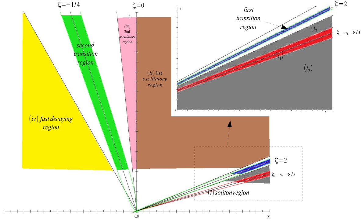
In [6], CH equation (1.1) has been transformed to its corresponding Riemann-Hilbert problem. The long time asymptotics can then be derived by using the nonlinear steepest descent method [18] and the isomonodromy method [20]. Four solution sectors and two transition regions have been found in the $\left(x,t>0\right)$ half-plane. The leading term of the long-time asymptotic solution $u\left(x,t\right)$ in each region behaves differently, depending on the slope, namely, $\zeta=\frac{x}{t}$ (see Figure 1).

$(i)$ $\zeta>2+\varepsilon$ for any $\varepsilon>0:$ soliton region,

$(ii)$ $0\leq\zeta<2-\varepsilon$ for any $\varepsilon>0:$ first oscillatory region,

$(iii)$ $\frac{-1}{4}+\varepsilon<\zeta<0$ for any $\varepsilon>0:$ second oscillatory region,

$(iv)$ $\zeta<\frac{-1}{4}-\varepsilon$ for any $\varepsilon>0:$ fast decay region.

Moreover, by [5], the following two transition regions exist for any $C>0:$

(1) $\left|\zeta-2\right|t^{\frac{2}{3}}<C$ (between the solution sectors $(i)$ and $(ii)$ shown in Figure 1),

(2) $\left|\zeta+\frac{1}{4}\right|t^{\frac{2}{3}}<C$ (between the solution sectors $(iii)$ and $(iv)$ shown in Figure 1).

Refer to caption — Figure 1: The long-time asymptotics of the CH solutions in the qualitatively different regions with $q_{0}=\frac{1}{2}$ . Then $c_{1}$ considered in the region (i) in Section 5.1 can be found as $c_{1}=\frac{8}{3}.$ Note that $\zeta$ is defined as $\zeta=\frac{x}{t}.$ For $\varepsilon=\frac{14}{80},$ the soliton region $(i)$ ( $\frac{x}{t}>2+\varepsilon$ ) which is the union of the red region $(i_{1})$ (between the lies $\frac{x}{t}=\frac{8}{3}-\varepsilon$ and $\frac{x}{t}=\frac{8}{3}+\varepsilon$ ) and the gray region $(i_{2})$ (two sectors, one is between the lines $\frac{x}{t}=2+\varepsilon$ and $\frac{x}{t}=\frac{8}{3}-\varepsilon,$ the other one is between the lines $\frac{x}{t}=\frac{8}{3}+\varepsilon$ and $t=0$ ).

Subject to the newly derived initial condition (3.1), the long-time asymptotic solutions in the six regions can then be expressed in terms of the scattering data (3.2) or equivalently in terms of the given parameter $q_{0}\in\left(0,1\right)$ appearing in (3.1). The details can be seen in the Appendix A. In the following, the solution of (1.1) is sought subject to (3.1) by applying the numerical scheme detailed in Section 4. The FDTD solution $u_{\text{num}}\left(x,t\right)$ will be compared with the asymptotic form of the solution expressed in terms of the scattering data (3.2) given in [6].

In Figure 2 the profile of the solution $u_{\text{num}}\left(x,t\right)$ predicted, for example, at $t=40$ is plotted with $q_{0}=\frac{1}{2}$ . In the rest of this paper we will numerically revisit these asymptotics summarized above in the physically distinct regions with $q_{0}=\frac{1}{2}$ .

5.1 Discussion of results in four regions $(i)$ - $(iv)$

5.1.1 Solution in the soliton region $(i)$

In the soliton region $\zeta>2+\varepsilon,$ $u\left(x,t\right)$ in $(i)$ behaves like a sole soliton due to the existence of a single discrete eigenvalue. Let $c_{1}=\frac{2}{1-4\mu_{1}^{2}}$ . For any $\varepsilon>0,$ the region $(i)$ can be divided into the following two subdomains (see [6] or the Appendix A):

$(i_{1})$ If $\left|\zeta-c_{1}\right|<\varepsilon$ ,

u\left(x,t\right)=u_{\text{sol}}^{1}\left(x,t\right)+O\left(t^{-l}\right)\text{ for any }l>0,

(5.1)

where $u_{\text{sol}}^{1}\left(x,t\right)$ is the 1-soliton solution and it can be expressed parametrically as (A.2) and (A.1) in the Appendix A with $j=1$ .

$(i_{2})$ If $\left|\zeta-c_{1}\right|\geq\varepsilon$ , $u\left(x,t\right)$ is rapidly decreasing.

According to (A.5) in the Appendix A, the dependence of the 1-soliton solution on the parameter $q_{0}$ can be clearly seen. Since $q_{0}=\frac{1}{2}$ , it can be found that $c_{1}=\frac{8}{3},$ and (A.5) takes the form as:

\left\{\begin{tabular}[]{l}$u\left(y,t\right)=\frac{4}{3}\frac{1}{\frac{5}{4}+\frac{3}{4}\left(e^{\frac{1}{2}\left(y-\frac{8}{3}t\right)}+\frac{1}{4}e^{\frac{-1}{2}\left(y-\frac{8}{3}t\right)}\right)},\vskip 6.0pt plus 2.0pt minus 2.0pt$\\ $x\left(y,t\right)=y+\log\frac{1+\frac{3}{2}e^{-\frac{1}{2}\left(y-\frac{8}{3}t\right)}}{1+\frac{1}{6}e^{-\frac{1}{2}\left(y-\frac{8}{3}t\right)}}.$\end{tabular}\right.

(5.2)

Equation (5.2) is valid in the region ( $i_{1}$ ): $\left|\frac{x}{t}-\frac{8}{3}\right|<\varepsilon$ . Take $\varepsilon=\frac{14}{80}$ as an example, at $t=80,$ the soliton region (A) shown in Figure 2 is known to fall in the region $(i_{1})$ , namely, $199.\,\allowbreak 33<x<227.\,\allowbreak 33$ . Outside this region, i.e., $x\geq 227.6633$ or $174<x\leq 199.33,$ $u\left(x,t\right)\sim 0.$ The numerically predicted solution $u_{\text{num}}\left(x,t\right)$ and the asymptotic solution $u_{\text{sol}}^{1}\left(x,80\right)$ in (5.2) are plotted in Figure 3. From (5.1), the decay of the difference between $u_{\text{num}}\left(x,t\right)$ and $u_{\text{sol}}^{1}\left(x,t\right)$ is sufficiently rapid with respect to time such that two solutions can match very well at $t=80.$ However, in region $(ii)$ the decay rate is relatively slow judging either from the previous result or from our numerical result in the following subsection.

5.1.2 Solution in the slowly decaying modulated oscillation region $(ii)$

In the first oscillatory region $0\leq\zeta=\frac{x}{t}<2-\varepsilon,$ the solution $u\left(x,t\right)$ takes the form as

u\left(x,t\right)=\frac{c_{1}^{\left(0\right)}}{\sqrt{t}}\sin\left(c_{2}^{\left(0\right)}t+c_{3}^{\left(0\right)}\log t+c_{4}^{\left(0\right)}\right)+O\left(t^{-\alpha}\right),

(5.3)

for any $\alpha\in\left(\frac{1}{2},1\right)$ provided $l\geq 5.$ $c_{n}^{\left(0\right)}$ ( $n=1,...,4$ ) are functions of $\zeta\$ depending on the reflection coefficient $R\left(k\right)$ (see [6] or the Appendix A).

At $t=40,80,160,200,$ and $\varepsilon=\frac{14}{80},$ the slowly decaying modulated oscillation region (B) shown in Figure 2 is known to be in the region of $0\leq x<73,0\leq x<146,0\leq x<292$ and $0\leq x<365$ , respectively. The numerically predicted solution and the asymptotic solution (5.3) are plotted in Figure 4.

By comparing the two formulas (5.1) and (5.3), it is clear that the decay order of the computed difference in the region $(i)$ is much larger than that in the region $(ii).$ Hence to get a good match between the two solutions in (5.3), the time span needs to be longer than that in region $(i)$ . This can be examined from Figure 4. We can see that at $t=80,$ although the numerical solution and the soliton solution in (5.2) match already very well in the soliton region $(i)$ in Figure 3, the numerical solution and the asymptotic solution in (5.3) have not matched well in regions with large $x$ in region $(ii)$ in Figure 4. We need, therefore, a longer time for example $t=200$ seen in Figure 4 to guarantee a good match between the numerical and the asymptotic solutions.

5.1.3 Solution in region $(iii)$ with the sum of two decaying modulated oscillations

In the second oscillatory region $\frac{-1}{4}+\varepsilon<\zeta=\frac{x}{t}<0,$ $u\left(x,t\right)$ behaves like

u\left(x,t\right)=\sum_{j=1}^{2}\frac{c_{1}^{\left(j\right)}}{\sqrt{t}}\sin\left(c_{2}^{\left(j\right)}t+c_{3}^{\left(j\right)}\log t+c_{4}^{\left(j\right)}\right)+O\left(t^{-\alpha}\right),

(5.4)

for any $\alpha\in\left(\frac{1}{2},1\right)$ provided $l\geq 5$ , where $c_{n}^{\left(j\right)}$ ( $n=1,...,4,$ $j=1,2$ ) are defined in the same way as $c_{n}^{\left(0\right)}$ .

At $t=40,80,160,200,$ and $\varepsilon=\frac{14}{80}$ , the slowly decaying modulated oscillation region (C) shown in Figure 2 is known to fall into $-3\leq x<0,-6\leq x<0,-12\leq x<0$ and $-15\leq x<0$ , respectively. The numerically predicted solution and the asymptotic solution in (5.4) are plotted in Figure 5. Similar to the solution in region $(ii)$ , we can see from Figure 5 that the numerical and asymptotic solutions become well matched until $t=200$ .

5.1.4 Solution in the fast decaying region $(iv)$

In the fast decaying region $\zeta=\frac{x}{t}<\frac{-1}{4}-\varepsilon,$ $u\left(x,t\right)$ behaves like

u\left(x,t\right)=O\left(t^{-l}\right)\text{ for any }l>0.

(5.5)

If we consider the case of $\varepsilon=\frac{14}{80},$ the fast decaying region (D) schematically shown in Figure 2 at $t=40,80,160,200$ occurs in the regions of $x<-17,x<-34,x<-68,x<-85,$ respectively. The numerically predicted solution and the zero (exact) solution are plotted in Figure 6.

Although the decay order of error in (5.5) is as large as that in region $(i)$ , by zooming the numerical and the asymptotic solution profiles, we can find from Figure 6 the difference between the regions $(i)$ and $(iv)$ . At $t=40,$ the numerical solution is not very close to zero for $x$ approaching the right end. Until $t=200,$ these two solutions can match well with each other for the vertical solution axis being scaled by $10^{-20}.$

5.2 Discussion of results in two Painlevé regions

The Painlevé equation of type II is given as

v^{\prime\prime}\left(s\right)=2v^{3}\left(s\right)+sv\left(s\right).

(5.6)

The one-parameter family of solutions to (5.6) was obtained firstly by Ablowitz and Segur [2] and then by Hastings and Mcleod [21] for $s\in\mathbb{R}.$ They considered the solutions of (5.6) as the solutions of a linear integral equation of the Gel’fand-Levitan type with a given $r\in\mathbb{R}$

K\left(s,\eta\right)=r\text{Ai}\left(\frac{s+\eta}{2}\right)+\frac{r^{2}}{4}\int_{s}^{\infty}\int_{s}^{\infty}K\left(s,\bar{\eta}\right)\text{Ai}\left(\frac{\bar{\eta}+\tilde{\eta}}{2}\right)\text{Ai}\left(\frac{\tilde{\eta}+\eta}{2}\right)d\bar{\eta}d\tilde{\eta}\text{.}

In the above, Ai $\left(s\right)$ is the Airy function. Then $v\left(s\right)\left(=v\left(s;r\right)=K\left(s,s\right)\right)$ satisfies (5.6) subject to the specified boundary condition $v\left(s;r\right)\sim r$ Ai $\left(s\right)$ as $s\rightarrow\infty,$ $s\in\mathbb{R}$ (see also [11]).

5.2.1 Solution in the first transition region (T1)

From [5], for $\left|\frac{x}{t}-2\right|t^{\frac{2}{3}}<C,$ $u\left(x,t\right)$ behaves like

u\left(x,t\right)=-\left(\frac{4}{3}\right)^{\frac{2}{3}}\frac{1}{t^{\frac{2}{3}}}\left(v^{2}\left(s\right)-v^{\prime}\left(s\right)\right)+O\left(t^{-1}\right),

(5.7)

where $s=6^{\frac{-1}{3}}\left(\frac{x}{t}-2\right)t^{\frac{2}{3}},$ and $v=v\left(s\right)=v\left(s;-R\left(0\right)\right)$ is the real valued, non-singular solution of (5.6) fixed by $v\left(s\right)\sim-R\left(0\right)$ Ai $\left(s\right)$ as $s\rightarrow\infty$ .

In the numerical computation of the Painlevé equation of type II, we use the connection formulas derived by [12, 21]. Since $R\left(0\right)=-1$ from the equation (3.2), by the Hastings and Mcleod’s result [21] the $P_{II}$ solution of equation (5.6) sought subject to the boundary condition $v\left(s\right)\sim-R\left(0\right)Ai\left(s\right)=Ai\left(s\right)$ is unique. Moreover, the asymptotic solution for $v$ can be expressed as $v\left(s\right)\sim\sqrt{\frac{-1}{2}s}$ as $s\rightarrow-\infty$ .

By choosing a large interval, say $\left(s_{L},s_{R}\right)$ with $s_{L}s_{R}<0,$ the solution of (5.6) sought subject to the boundary condition $v\left(s_{L}\right)=\sqrt{\frac{-1}{2}s_{L}},$ $v\left(s_{R}\right)=Ai\left(s_{R}\right)=\frac{1}{2\sqrt{\pi}}\left(s_{R}\right)^{\frac{-1}{4}}e^{\frac{-2}{3}\left(s_{R}\right)^{\frac{3}{2}}}\$ can be obtained. This solution is called as $v_{2}\left(s\right).$

If the case with $C=\frac{14}{80}$ is considered, the first transition region (T1) schematically shown in Figure 2 at $t=80$ and $160$ is defined in the regions of $159.25<x<160.75,$ $320.95<x<319.05,$ respectively. The numerically predicted solution and the leading term of the asymptotic solution shown in (5.7) with $v=v_{2}\left(s\right)$ are plotted in Figure 7.

We can then compare the leading term of the asymptotic solution (5.7) with $v=v_{2}\left(s\right)$ and $u\left(x,t\right)$ at, for example, $t=40.$ This corresponds to compare the finite difference solution $u\left(x,40\right)$ and the following term

-\left(\frac{4}{3}\right)^{\frac{2}{3}}\frac{1}{t^{\frac{2}{3}}}\left(v_{2}^{2}\left(s\right)-v_{2}^{\prime}\left(s\right)\right).

(5.8)

Figure 7 exhibits a perfect agreement between the two graphs for the numerical solution and the asymptotic solution (5.8) expressed in terms of $v_{2}\left(s\right)$ at $t=160.$

5.2.2 Solution in the second transition region (T2)

From [5], for $\left|\frac{x}{t}+\frac{1}{4}\right|t^{\frac{2}{3}}<C,$ $u\left(x,t\right)$ has been derived as

u\left(x,t\right)=\frac{12^{\frac{1}{6}}}{t^{\frac{1}{3}}}v_{1}\left(s_{1}\right)\sin\psi\left(s_{1},t\right)+O\left(t^{-\frac{2}{3}}\right),

(5.9)

where $s_{1}=-\left(\frac{16}{3}\right)^{\frac{1}{3}}\left(\frac{x}{t}+\frac{1}{4}\right)t^{\frac{2}{3}}$ and $v_{1}\left(s\right)=v_{1}\left(s;\left|R\left(\frac{\sqrt{3}}{2}\right)\right|\right)$ is the real valued, non-singular solution of (5.6) fixed by $v_{1}\left(s\right)\sim\left|R\left(\frac{\sqrt{3}}{2}\right)\right|Ai\left(s\right)$ as $s\rightarrow\infty$ . Other notations shown in (5.9) and their $q_{0}$ -dependence can be seen in the Appendix A.

Since $\left|R\left(\frac{\sqrt{3}}{2}\right)\right|<1$ , by the Clarkson and Mcleod’s result [12] the solution of the $P_{II}$ equation (5.6) obtained under the boundary condition $v\left(s\right)\sim\left|R\left(\frac{\sqrt{3}}{2}\right)\right|$ Ai $\left(s\right)$ is unique. Moreover, the corresponding asymptotic behavior for $v$ as $s\rightarrow-\infty$ can be expressed as

v\left(s\right)\sim d\left|s\right|^{\frac{-1}{4}}\sin\left\{\frac{2}{3}\left|s\right|^{\frac{3}{2}}-\frac{3}{4}d^{2}\ln\left|s\right|-\theta_{0}\right\}\text{ as }s\rightarrow-\infty,

(5.10)

where $d$ and $\theta_{0}$ can be seen in [12] and their $q_{0}$ -dependence can be seen in the Appendix A.

By choosing a large interval, say $\left(\hat{s}_{L},\hat{s}_{R}\right)$ with $\hat{s}_{L}\hat{s}_{R}<0,$ the solution of (5.6) with the boundary condition $v\left(\hat{s}_{L}\right)=B_{-}\left(\hat{s}_{L}\right),$ $v\left(\hat{s}_{R}\right)=B_{+}\left(\hat{s}_{R}\right)$ (see (A.8) in the Appendix A) can be obtained. We call this solution as $v_{3}\left(s\right).$

At $C=\frac{14}{80}$ , the second transition region (T2) schematically shown in Figure 2 at $t=80$ and $160$ falls in the regions of $-20.754<x<-19.246$ and $-40.95<x<-39.05,$ respectively. The numerically predicted solution and the leading term of the asymptotic solution taking the form of (5.9) with $v=v_{3}\left(s\right)$ are plotted in Figure 8.

Based on the similar argument to the one presented in the first Painlevé region, the predicted solution $u\left(x,t\right)$ can be now compared with the leading term (5.9) of the Painlevé II solution

\frac{12^{\frac{1}{6}}}{t^{\frac{1}{3}}}v_{3}\left(s_{1}\right)\sin\psi\left(s_{1},t\right)\text{.}

(5.11)

In Figure 8, at $t=160$ we can see a good agreement between the two graphs of the numerical solution and the asymptotic solution (5.11) expressed in terms of $v_{3}\left(s\right)$ .

5.3 The $\varepsilon-$ and $C-$ dependence in the asymptotic regions

Both $\varepsilon$ and $C$ appeared in the beginning of this section can characterize the regions of different solution behaviors. In the $\left(x,t>0\right)$ plane, the $\varepsilon$ appeared in the four regions $(i)$ - $(iv)$ characterizes the degree of the departure from the two lines $\frac{x}{t}=2$ and $\frac{x}{t}=\frac{-1}{4}$ . The constant $C$ present in the two transition regions characterizes the degree of departure from the lines $\frac{x}{t}=2$ and $\frac{x}{t}=\frac{-1}{4}.$

In Figure 9 we plot the variance of the asymptotic regions for $C=\frac{14}{80}$ and $\varepsilon=\frac{10}{80},\frac{14}{80}$ and $\frac{18}{80}$ , respectively. From the result in [6] (see the Appendix A), let us take the regions $(iii)$ and $(iv)$ as an example for the discussion of results in Figure 9. For $C$ being fixed at $\frac{14}{80}$ , given a large enough $\varepsilon$ , the regions $(iii)$ $\frac{-1}{4}+\varepsilon<\frac{x}{t}<0$ and $(iv)$ $\frac{x}{t}<\frac{-1}{4}-\varepsilon$ will exhibit oscillatory asymptotics. However, as $\varepsilon$ becomes smaller, regions $(iii)$ and $(iv)$ become larger, and at the same time regions $(iii)$ and $(iv)$ are closer to the second transition region $\left|\frac{x}{t}+\frac{1}{4}\right|t^{\frac{2}{3}}<C$ . As long as $t$ is sufficiently large, the condition $Ct^{\frac{-2}{3}}<\varepsilon$ can be satisfied no matter what the chosen values of $\varepsilon$ and $C$ are. That is, the transition region (T2) will not affect the regions $(iii)$ and $(iv)$ for $t$ being larger enough for any choice of $\varepsilon$ and $C.$ One should notice that in figure (c) of Figure 9, the region with white color between the region $(iii)$ and the region (T2) can not be considered as a region belonging to neither the region $(iii)$ nor the region (T2). In fact, this white region should be regarded as the region $(iii)$ with $\varepsilon$ becoming greater than $\frac{18}{80}.$ Other white regions in different places can be argued by a similar way.

5.4 Discussion of the time-decay estimates

In questions (Q1) and (Q2), we are asked ourselves how to determine the time that is long enough that the predicted solution has matched with asymptotic solution and how to obtain the powers of $t$ in the time-decay estimates under the specified initial data (3.1). In this section, we are aimed to answer these two questions in the following way. Let $u_{j}\left(x,t\right)$ with $j=$ 1,…,4, 5 and 6 be the asymptotic solutions in regions $(i)$ ,…, $(iv)$ and in the first and the second transition regions, respectively. Let $I_{j}$ with $j=$ 1,…,4, 5 and 6 denoting the regions $(i)$ ,…, $(iv)$ and the first and the second transition regions, respectively.

In Subsection 5.4.1 we find the time $T_{j}$ in each $I_{j}$ such that the difference between the numerical solution $u_{\text{num}}\left(x,t\right)$ and the asymptotic solution $u_{j}\left(x,t\right)$ becomes small enough for $t\geq T_{j}.$ Here ”small enough” between $u_{\text{num}}\left(x,t\right)$ and $u_{j}\left(x,t\right)$ solutions is measured by considering the $L^{2}$ norm difference between $u_{\text{num}}\left(x,t\right)$ and $u_{j}\left(x,t\right)$ in each region $I_{j}:$

E_{j}^{L2}\left(t\right):=\left(\int_{I_{j}}\left|u_{\text{num}}\left(x,t\right)-u_{j}\left(x,t\right)\right|^{2}dx\right)^{\frac{1}{2}}

for $j=$ 1,…,4, 5 and 6. We find the time $T_{j}$ in each $I_{j}$ such that $E_{j}^{L2}\left(t\right)$ becomes small and there is no significant variation any longer for $t\geq T_{j}.$ Then the time needed for the computed solutions to reach the asymptotics can be found in each region $I_{j}$ .

In Subsection 5.4.2, the decay order theoretically derived from [6] will be calculated in a numerical way. Let $E_{j}^{\sup}\left(t\right):=\max_{x\in I_{j}}\left|u_{\text{num}}\left(x,t\right)-u_{j}\left(x,t\right)\right|.$ Based on the point-wise sense of the asymptotic formulas (5.1), (5.3), (5.4) and (5.5) in [6], the function space considered for (Q2) is different from that in Subsection 5.4.1. The exact power of $t$ in these asymptotic formulas remains unknown in [6]. The above mentioned question (Q2) concerns the way of computing the value of the power of $t.$

In Subsection 5.4.3, we discuss the influence of the range considered in each region on the computed decay rates. The result shows that if a larger region is considered, the time needed to reach the long-time asymptotics will be longer accordingly. That is, the computed decay rates will become smaller.

5.4.1 The predicted long time in each region

We find the time needed to reach the asymptotics by computing $E_{j}^{L2}\left(t\right)$ in each $I_{j}$ ( $j=2$ , $3$ , $4$ ).

Figure 10 plots the time-decay profiles of $E_{j}^{L2}\left(t\right)$ in regions $(i)$ - $(iv)$ at different times with $\varepsilon=\frac{14}{80}$ . In region $(iii)$ , for a large enough $t$ , the estimate $E_{3}^{L2}\left(t\right)$ becomes sufficiently small. In regions $(i)$ and $\left(iv\right)$ , the decay orders are much larger than those in regions $(ii)$ and $(iii)$ from these graphs. Moreover, the variances of $E_{j}^{L2}\left(t\right)$ ( $j=1,$ $2$ , $3$ , $4$ ) are tabulated in Table 1.

$t$	$E_{1}^{L2}(t)$	$E_{2}^{L2}\left(t\right)$	$E_{3}^{L2}\left(t\right)$	$E_{4}^{L2}\left(t\right)$
$40$	1.303304031375658E-2	0.292954164986533	1.612163792174788E-2	1.442232517777524E-4
$80$	4.170394908225294E-3	0.200463612016154	5.009588123729806E-3	2.575958816177057E-6
$120$	1.557160720783265E-3	0.171595918602204	4.443772185385986E-3	5.457070673560806E-8
$160$	6.124634754925668E-4	0.177361156697756	4.289889498025333E-3	1.163202136797550E-9
$200$	2.498850932347651E-4	0.187198259978890	4.372113314984243E-3	2.755050865021234E-11
$240$	1.060794858467605E-4	0.191131350654329	3.944857443413838E-3	6.595925065534878E-13
$280$	5.032093370750756E-5	0.190235716309735	3.837028523022252E-3	1.572983122931371E-14
$320$	3.113956434979408E-5	0.191477176087681	3.890293609233680E-3	3.709034000389790E-16
$360$	2.655384864147633E-5	0.195600653012653	3.727629679179258E-3	8.614729075722736E-18
$400$	2.575663036324579E-5	0.191706872966999	3.802122218224038E-3	1.966797275673494E-19

Table 1: The differences

E_{j}^{L2}\left(t\right)

(

j=1,2,3,4

) obtained in the regions

(i)-(iv)

at different times for

\varepsilon=\frac{14}{80}

Motivated by the fact given in [6] that the decay orders in regions $(ii)$ and $(iii)$ are smaller than those in regions $(i)$ and $(iv),$ we focus on the closeness between the numerical and the asymptotic solutions in regions $(ii)$ and $(iii).$ That is, in a shorter time, the analytical solutions already match the asymptotic solutions very well in regions $(i)$ and $(iv).$ Therefore $\min\left\{T_{2},T_{3}\right\}>\max\left\{T_{1},T_{4}\right\}$ and the long time $T:=\max_{1\leq j\leq 4}T_{j}$ stated above needs to be found by examining $T_{2}$ and $T_{3}$ in regions $(ii)$ and $(iii)$ , respectively.

In Table 1 and Figure 10, we take $T_{1}=160,$ $T_{3}=240$ and $T_{4}=40$ as the respective times at which the numerical solutions match very well with the asymptotic solutions in regions $(i),$ $(iii)$ and $(iv)$ . However, $T_{2}$ can not determined easily from the graph in Figure 10. We choose $T_{2}=280$ and the reason will be explained in the next section.

5.4.2 The numerically computed decay powers of $t$

In this subsection we consider the powers of $t$ of the time-decay estimates in [6].

Figure 11 plots the time-decay profiles of the sup norm $E_{j}^{\sup}\left(t\right)$ in regions $(i)$ - $(iv)$ , respectively, at different times with $\varepsilon=\frac{14}{80}$ . Similar to the $L^{2}$ norm results, in regions $(ii)$ and $(iii)$ the estimates $E_{2}^{\sup}\left(t\right)$ and $E_{3}^{\sup}\left(t\right)$ become small enough for a large enough $t$ . The decay orders in regions $(i)$ and $\left(iv\right)$ look much larger than those in regions $(ii)$ and $(iii)$ . Moreover, the variances of $E_{j}^{\sup}\left(t\right)$ ( $j=1,$ $2$ , $3$ , $4$ ) are tabulated in Table 2.

$t$	$E_{1}^{\sup}(t)$	$E_{2}^{\sup}\left(t\right)$	$E_{3}^{\sup}\left(t\right)$	$E_{4}^{\sup}\left(t\right)$
$40$	8.468787040579530E-3	1.40463349496939E-1	4.526819459939539E-2	1.802887487030715E-4
$80$	2.562851596378625E-3	8.675408665040811E-2	4.496098688352251E-3	3.742290026355494E-6
$120$	9.354531544216522E-4	4.260921144987524E-2	4.144216057718784E-3	8.745510811409106E-8
$160$	3.636038798000425E-4	3.965394156144474E-2	3.566372610309353E-3	1.911307301562621E-9
$200$	1.467776857832571E-4	3.840181001023902E-2	3.306124437020473E-3	4.524112000962450E-11
$240$	6.063916391485836E-5	3.724938756956186E-2	2.548191267527537E-3	1.048626564931299E-12
$280$	2.565702741164118E-5	3.619659640699480E-2	2.513406195082118E-3	2.373955192058340E-14
$320$	1.755075330411859E-5	3.523470929795400E-2	2.352826688157257E-3	5.235427733097183E-16
$360$		3.435271074529302E-2	2.311665267575798E-3	1.120502174844415E-17
$400$		3.354081711805757E-2	2.030974658791331E-3	2.318829978373335E-19

Table 2: The differences

E_{j}^{\sup}\left(t\right)

(

j=1,2,3,4

) obtained in the regions

(i)-(iv)

at different times for

\varepsilon=\frac{14}{80}

In the following the question (Q2) will be answered by two means. In other words, the decay order of the estimate $E_{j}^{\sup}\left(t\right)$ will be found numerically under two different error estimates:

(1) The rates of convergence (R.O.C.) in regions $(ii)$ - $(iv)\$ are computed. The results are summarized in Table 3.

region $(ii)$	region $(iii)$	region $(iv)$
0.7998085	0.5159832	13.1137

Table 3: The computed rates of convergence in the regions

(ii)

(iii)

and

(iv)

(2) In [6], the decay orders in the regions $\left(i\right)$ and $(iv)$ are $O\left(t^{-l}\right)\$ while $O\left(t^{-\alpha}\right)$ in the regions $(ii)$ and $(iii)$ for any $\alpha\in\left(\frac{1}{2},1\right)$ provided $l\geq 5$ (see (5.1), (5.3), (5.4) and (5.5)). Therefore there exist four different constants $C_{i}$ such that

E_{j}^{\sup}\left(t\right)\leq C_{j}t^{-l_{j}}

for

j=1,4;\vskip 3.0pt plus 1.0pt minus 1.0pt

E_{j}^{\sup}\left(t\right)\leq C_{j}t^{-\alpha_{j}}

for

j=2,3.

(5.12)

Note that $C_{j}$ $(j=1,...,4)$ are independent of $t$ . In the following we numerically calculate the decay orders in the regions $(i)$ - $(iv)$ .To this end, we first define the numerically computed decay powers in the regions $(i)$ - $(iv).$

Definition 5.1.

Let $T=\max\left\{T_{1},...,T_{4}\right\}$ be the maximum of the long times $T_{1},...,T_{4}$ found in question (Q1). The numerical decay powers $L_{1},$ $L_{4}$ , $A_{2}$ and $A_{3}$ are defined to be the values such that

E_{j}^{\sup}\left(T\right)=T^{-L_{j}},\text{ }j=1,4;\text{ \ }E_{j}^{\sup}\left(T\right)=T^{-A_{j}},\text{ }j=2,3.

That is,

L_{1,4}=-\frac{\log E_{1,4}^{\sup}\left(T\right)}{\log T},\ A_{2,3}=-\frac{\log E_{2,3}^{\sup}\left(T\right)}{\log T}.

The values $L_{1},$ $L_{4}$ , $A_{2}$ and $A_{3}$ are considered to be the powers of $t$ of the time-decay estimates measured by the sup norm between the numerical solution and the asymptotic solution.

One of the difficulties of computing the decay orders is that the values $C_{j}$ in (5.12) can not be found theoretically. As a result, we suppose $C_{j}=1$ in Definition 5.1.

From the results in (Q1), we have $T=\max\left\{T_{1},...,T_{4}\right\}=280.$ Then from Table 2, $L_{1},$ $L_{4}$ , $A_{2}$ and $A_{3}$ can be found as

L_{1}=-\frac{\log E_{1}^{\sup}\left(T\right)}{\log T}=\frac{-\log\left(6.063916391485836\times 10^{-5}\right)}{\log 240}=1.7718,

A_{2}=-\frac{\log E_{2}^{\sup}\left(T\right)}{\log T}=\frac{-\log\left(3.619659640699480\times 10^{-3}\right)}{\log 280}=0.99762,

A_{3}=-\frac{\log E_{3}^{\sup}\left(T\right)}{\log T}=\frac{-\log\left(2.513406195082118\times 10^{-3}\right)}{\log 280}=1.0623,

L_{4}=-\frac{\log E_{4}^{\sup}\left(T\right)}{\log T}=\frac{-\log\left(2.373955192058340\times 10^{-14}\right)}{\log 280}=5.5675.

Remark According to the results, we can see that the numerical decay powers match the restrictions of the powers of $t$ in regions $(ii)$ and $(iv)$ from [6]. The reason for choosing $T_{2}=280$ is therefore explained. We can further compute $A_{2}$ at different times by

\left.A_{2}\right|_{t=240}=-\frac{\log E_{2}^{\sup}\left(240\right)}{\log 240}=\frac{-\log\left(3.724938756956186\times 10^{-3}\right)}{\log 240}=1.0204.

For the determination of $T$ in the question (Q1), Figure 10 is not sufficient to answer this question. We need the predicted numerical decay power since at $t=280$ the corresponding $A_{2}$ can match the result $\alpha\in\left(\frac{1}{2},1\right)$ in [6]. Moreover, in region $(iii),$ at $t=400,$ one can find that $A_{3}=\frac{-\log\left(2.030974658791331\times 10^{-3}\right)}{\log 400}=1.0347.$ This value is close to the power of $t$ in (5.4).

5.4.3 The dependence of the numerical decay powers on $\varepsilon$

In order to compare the influence of the chosen $\varepsilon$ on $E_{j}^{\sup}\left(t\right),$ the variances of $E_{j}^{\sup}\left(t\right)$ ( $j=2$ , $4$ ) obtained at different $\varepsilon$ are tabulated in Table 4.

	$t$	$\varepsilon=\frac{9}{80}$	$\varepsilon=\frac{14}{80}$	$\varepsilon=\frac{19}{80}$
	$40$	1.418562E-1	1.404633E-1	1.180903E-1
$E_{2}^{\sup}\left(t\right)$	$80$	1.048379E-1	8.67541E-2	4.211969E-2
	$120$	8.665302E-2	4.26092E-2	4.09646E-2
	$160$	7.31637E-2	3.96539E-2	3.96539E-2
	$200$	5.899846E-2	3.84018E-2	3.84018E-2
	$240$	4.469613E-2	3.724938E-2	3.724938E-2
	$280$	3.619659E-2	3.61965E-2	3.619659E-2
	$320$	3.523470E-2	3.52347E-2	3.52347E-2
	$40$	1.319865E-3	1.80288E-4	2.801281E-5
$E_{4}^{\sup}\left(t\right)$	$80$	1.783843E-4	3.74229E-6	6.24902E-8
	$120$	1.783843E-5	8.745510E-8	5.18444E-10
	$160$	1.783843E-6	1.91130E-9	6.47375E-13
	$200$	1.783843E-7	4.52411E-11	5.59605E-15
	$240$	1.783843E-8	1.04862E-12	6.87049E-18
	$280$	1.783843E-9	2.373955E-14	2.463507E-20
	$320$	1.783843E-10	5.235427E-16	8.57598E-24

Table 4: The differences

E_{2}^{\sup}\left(t\right)

and

E_{4}^{\sup}\left(t\right)

obtained in the regions

(ii)

and

(iv)

, respectively at different times for

\varepsilon=\frac{9}{80},

\varepsilon=\frac{14}{80},

\varepsilon=\frac{19}{80}

$t$	$A_{2}$ at $\varepsilon=\frac{9}{80}$	$A_{2}$ at $\varepsilon=\frac{14}{80}$	$A_{2}$ at $\varepsilon=\frac{19}{80}$
$40$	$0.52941$	$0.53209$	$0.57912$
$80$	$0.51468$	$0.55789$	$0.72278$
$120$	$0.51088$	$0.65915$	$0.66737$
$160$	$0.51526$	$0.63595$	$0.63595$
$200$	$0.53418$	$0.61522$	$0.61522$
$240$	$0.56706$	$0.60032$	$0.60032$
$280$	$0.58898$	$0.58898$	$0.58898$
$320$	$0.58002$	$0.51139$	$0.58002$

Table 5: The numerical decay rate

A_{2}

in region

(ii)

computed from the differences tabulated in Table 4 at different

t.

$t$	$L_{4}$ at $\varepsilon=\frac{9}{80}$	$L_{4}$ at $\varepsilon=\frac{14}{80}$	$L_{4}$ at $\varepsilon=\frac{19}{80}$
$40$	$1.7974$	$2.337$	$2.8417$
$80$	$1.9698$	$2.8516$	$3.7855$
$120$	$2.2839$	$3.3947$	$4.4658$
$160$	$2.6081$	$3.9556$	$5.53$
$200$	$2.9329$	$4.4956$	$6.1938$
$240$	$3.2554$	$5.0329$	$7.2107$
$280$	$3.575$	$5.5675$	$8.0127$
$320$	$3.8914$	$6.0999$	$9.2077$

Table 6: The numerical decay rate

L_{4}

in region

(iv)

computed from the differences tabulated in Table 4 at different

t.

Moreover, we list in Tables 5 and 6 different values of the numerical decay powers $A_{2}$ and $L_{4}$ predicted at different $\varepsilon$ in regions $(ii)$ and $(iv)$ , respectively. From these tables, the following conclusions can be drawn:

(1) In a single region, for a smaller $\varepsilon,$ the difference of the norms becomes larger. A smaller $\varepsilon$ means a larger region ( i.e., a higher precision) for the approximation under consideration. Therefore the time needed for the asymptotic solution to match the numerical solution is longer.

(2) For $\varepsilon=\frac{9}{80}$ , we compare the decay estimates $E_{2}^{\sup}\left(t\right)$ and $E_{4}^{\sup}\left(t\right)$ at the large time, say at $t=320.$ Then it follows that ${\small E}_{2}^{\sup}\left(320\right)>{\small E}_{4}^{\sup}\left(320\right).$ This important message sheds light on the decay sup norm difference in the region $(iv)$ , which is smaller than that in the region $(ii).$ This result matches the theoretical theorem obtained in [6], where the decay power $\alpha$ in region $(ii)$ satisfies $\alpha\in\left(\frac{1}{2},1\right)$ provided that the decay power $l$ in region $(iv)$ satisfies $l\geq 5.$ This means that the decay order in region $(iv)$ is larger than that in region $(ii)$ .

6 Concluding remarks

In this article we are aimed to get the long-time asymptotics for the CH equation (1.1). To this end, a new analytical initial condition (3.1) of the CH equation is constructed first underlying the scattering theory. It is worthy to note that this newly derived initial condition has a non-zero reflection coefficient. In the second part of this study, a new high-order finite difference scheme is developed and we apply it to solve the CH solution under the specified initial condition (3.1). Unlike the works of [6, 5], we quantitatively determine the asymptotic time $T\$ by considering the $L^{2}$ norm differences between the numerical and the asymptotic solutions. Beyond $T$ the predicted solutions approach the so called long-time asymptotic solutions in the six distinct regions (the four regions $(i)$ - $(iv)$ and the two transition regions) under current investigation. The value of $T$ depends strongly on how large the $\left(x,t>0\right)$ plane is required to get a good match between the numerical and asymptotic solutions.

Under the non-reflectionless condition, we have numerically revisited the oscillatory behaviors in the first and second oscillatory regions. Moreover, we can clearly see that the investigated spatial domain contains different asymptotic regions. The difference between the numerical and asymptotic solutions is also intensively examined. Moreover, the rates of convergence in different solution regions have been obtained as well. The decay orders of the time-decay estimates between the numerical and asymptotic solution in [6] are computed numerically by considering the sup norm difference between them. We have also computed the sup norm differences at different $\varepsilon$ , (i.e., at different amounts of area) in each region. For a larger $\varepsilon,$ the sup norm difference becomes smaller and the decay orders numerically computed will be larger. These numerical works are new to the best of authors’ knowledge.

It can be expected that as long as the specified initial solution of the integrable systems (including the CH equation, which is the example in this article) can be constructed, the corresponding time evolving solutions can be found by applying the currently developed numerical methods. Through this study, not only the long time behavior of the CH solution but also the short time solution profile predicted from the finite difference method can be obtained.

Appendix A Appendix

A.1 Previous results

Proposition A.1.

(Theorem 2.1 in [6]) Let $u\left(x,t\right)$ be the solution of (1.1), (1.2). There are four sectors in the $\left(x,t>0\right)$ half-plane. The leading term of the long-time asymptotics of $u\left(x,t\right)$ in each sector behaves differently depending on the magnitude of $\zeta=\frac{x}{t}:$ (see Figure 1).

(i) The soliton region: $\zeta>2+\varepsilon$ ( $\varepsilon>0$ small). Let

\alpha_{j}\left(y,t\right)=\frac{\gamma_{j}^{2}}{2\mu_{j}}e^{-2\mu_{j}\left(y-c_{j}t\right)},\text{ where }c_{j}=\frac{2}{1-4\mu_{j}^{2}},

(A.1)

with $j=1,...,N$ for some $N\in\mathbb{N}.$ Let $\varepsilon>0$ be a small enough magnitude such that $\left[c_{j}-\varepsilon,c_{j}+\varepsilon\right]$ and $\left[c_{j}-\varepsilon,c_{j}+\varepsilon\right]$ ( $i,j=1,...,N,$ $i\neq j$ ) are disjoint and are inside of $\left(2,\infty\right).$

(i₁) If $\left|\zeta-c_{j}\right|<\varepsilon$ for some $j,$ $u\left(x,t\right)$ behaves as the sum of 1-solitons. That is,

u\left(x,t\right)=u_{\text{sol}}^{j}\left(x,t\right)+O\left(t^{-l}\right)\text{ for any }l>0,

where $u_{\text{sol}}^{j}\left(x,t\right)$ is the 1-soliton and can be expressed parametrically in the form as follows

u\left(y,t\right)=\frac{32\mu_{j}^{2}}{\left(1-4\mu_{j}^{2}\right)^{2}}\frac{\alpha_{j}\left(y,t\right)}{\left(1+\alpha_{j}\left(y,t\right)\right)^{2}+\frac{16\mu_{j}^{2}}{1-4\mu_{j}^{2}}\alpha_{j}\left(y,t\right)},

\ \ x\left(y,t\right)=y+\log\frac{1+\alpha_{j}\left(y,t\right)\frac{1+2\mu_{j}}{1-2\mu_{j}}}{1+\alpha_{j}\left(y,t\right)\frac{1-2\mu_{j}}{1+2\mu_{j}}}

(A.2)

In the above, $\mu_{j}$ is one of the discrete eigenvalues with the corresponding normalization constant $\gamma_{j},$ $j=1,2,...,N$ ,

(i₂) If $\left|\zeta-c_{j}\right|\geq\varepsilon$ for all $j,$ $u\left(x,t\right)$ is rapidly decreasing;

(ii) The “first oscillatory” region: if $0\leq\zeta<2-\varepsilon$ for any $\varepsilon>0,$ $u\left(x,t\right)$ satisfies (5.3). That is,

u\left(x,t\right)=-\sqrt{\frac{2k_{0}\left(\zeta\right)\nu_{0}\left(\zeta\right)}{\left(\frac{1}{4}+k_{0}^{2}\left(\zeta\right)\right)\left(\frac{3}{4}-k_{0}^{2}\left(\zeta\right)\right)t}}\sin\left(\frac{2k_{0}^{3}\left(\zeta\right)}{\left(\frac{1}{4}+k_{0}^{2}\left(\zeta\right)\right)^{2}}t-\nu_{0}\left(\zeta\right)\log t+\delta_{0}\left(\zeta\right)\right)+O\left(t^{-\alpha}\right)

(A.3)

for any $\alpha\in\left(\frac{1}{2},1\right)$ provided $l\geq 5$ . The notations $k_{0},\nu_{0}$ and $\delta_{0}$ in this formula can be seen as well in [6] and their $q_{0}$ -dependence can be seen in Subsection A.2;

(iii) The “second oscillatory” region: if $\frac{-1}{4}+\varepsilon<\zeta<0$ for any $\varepsilon>0,$ $u\left(x,t\right)$ satisfies (5.4). That is,

$u\left(x,t\right)=$	$-\sqrt{\frac{2k_{0}\left(\zeta\right)\nu_{0}\left(\zeta\right)}{\left(\frac{1}{4}+k_{0}^{2}\left(\zeta\right)\right)\left(\frac{3}{4}-k_{0}^{2}\left(\zeta\right)\right)t}}\sin\left(\frac{2k_{0}^{3}\left(\zeta\right)}{\left(\frac{1}{4}+k_{0}^{2}\left(\zeta\right)\right)^{2}}t-\nu_{0}\left(\zeta\right)\log t+\bar{\delta}_{0}\left(\zeta\right)\right)$
	$-\sqrt{\frac{2k_{1}\left(\zeta\right)\nu_{1}\left(\zeta\right)}{\left(\frac{1}{4}+k_{1}^{2}\left(\zeta\right)\right)\left(k_{1}^{2}\left(\zeta\right)-\frac{3}{4}\right)t}}\sin\left(\frac{2k_{1}^{3}\left(\zeta\right)}{\left(\frac{1}{4}+k_{1}^{2}\left(\zeta\right)\right)^{2}}t+\nu_{1}\left(\zeta\right)\log t-\delta_{1}\left(\zeta\right)\right)+O\left(t^{-\alpha}\right)$

(A.4)

for any $\alpha\in\left(\frac{1}{2},1\right)$ provided $l\geq 5$ . The notations $k_{j},\nu_{j}$ ( $j=0,1$ ), $\bar{\delta}_{0}$ and $\delta_{1}$ in this formula can be seen in [6]. Their $q_{0}$ -dependence can be also seen in Subsection A.2;

(iv) The “fast decay” region: if $\zeta<\frac{-1}{4}-\varepsilon$ for any $\varepsilon>0,$ $u\left(x,t\right)$ is rapidly decreasing.

A.2 Newly derived long-time asymptotics

A.2.1 Region $(i)$

Substituting the derived scattering data $R\left(k\right)$ or (3.2) (i.e., $\mu_{j}=\mu_{1},$ $\gamma_{j}=\gamma_{1}$ ) into (A.2) and (A.1), the 1-soliton type of solution is expressed as

\left\{\begin{tabular}[]{l}$u\left(y,t\right)=\frac{4q_{0}^{2}}{\left(1-q_{0}^{2}\right)^{2}}\frac{1}{\exp\left(q_{0}\left(y-\frac{2}{1-q_{0}^{2}}t\right)\right)+\frac{1}{4}\exp\left(-q_{0}\left(y-\frac{2}{1-q_{0}^{2}}t\right)\right)+\frac{1+q_{0}^{2}}{1-q_{0}^{2}}},\vskip 6.0pt plus 2.0pt minus 2.0pt$\\ $x\left(y,t\right)=y+\log\frac{1+\exp\left(-q_{0}\left(y-\frac{2}{1-q_{0}^{2}}t+\frac{1}{q_{0}}\log 2\right)\right)\frac{1+q_{0}}{1-q_{0}}}{1+\exp\left(-q_{0}\left(y-\frac{2}{1-q_{0}^{2}}t+\frac{1}{q_{0}}\log 2\right)\right)\frac{1-q_{0}}{1+q_{0}}}.$\end{tabular}\right.

(A.5)

A.2.2 Region $(ii)$

By Proposition A.1, for $0\leq\zeta=\frac{x}{t}<2-\varepsilon$ the solution $u\left(x,t\right)$ behaves like (A.3), where $k_{0}\left(\zeta\right)=\frac{1}{2}\sqrt{-\frac{1+\zeta-\sqrt{1+4\zeta}}{\zeta}},$ $\nu_{0}\left(\zeta\right)=-\frac{1}{2\pi}\log\left(1-\left|R\left(k_{0}\left(\zeta\right)\right)\right|^{2}\right).$ Note that $\delta_{0}\left(\zeta\right)$ is expressed in (2.13) of [6]. Subject to the initial solution (3.1) and the corresponding scattering data (3.2), the asymptotic form (5.3) depends on the parameter $q_{0}$ in the sense of

\nu_{0}\left(\zeta\right)=-\frac{1}{2\pi}\log\frac{\sqrt{1+4\zeta}-1-\zeta}{\zeta q_{0}^{2}+\sqrt{1+4\zeta}-1-\zeta},

and

$\delta_{0}\left(\zeta\right)$	$=\frac{\pi}{4}-\left(\tan^{-1}\left(\frac{-2k_{0}\left(\zeta\right)}{q_{0}}\right)+\pi\right)-\nu_{0}\left(\zeta\right)\log\frac{32\zeta\left(\sqrt{1+4\zeta}-1-\zeta\right)\left(1+4\zeta-\sqrt{1+4\zeta}\right)}{\left(\sqrt{1+4\zeta}-1\right)^{3}}\vskip 3.0pt plus 1.0pt minus 1.0pt$
	$+4\tan^{-1}\left(\frac{q_{0}}{2k_{0}\left(\zeta\right)}\right)+4k_{0}\left(\zeta\right)\log\frac{1+q_{0}}{1-q_{0}}+\frac{4k_{0}\left(\zeta\right)}{\pi}\int_{-k_{0}\left(\zeta\right)}^{k_{0}\left(\zeta\right)}\frac{1}{1+4\xi^{2}}\log\frac{4\xi^{2}}{q_{0}^{2}+4\xi^{2}}d\xi\vskip 3.0pt plus 1.0pt minus 1.0pt$
	$+\frac{1}{\pi}\int_{-k_{0}\left(\zeta\right)}^{k_{0}\left(\zeta\right)}\frac{2q_{0}^{2}}{\left(q_{0}^{2}+4\xi^{2}\right)\xi}\log\left(k_{0}\left(\zeta\right)-\xi\right)d\xi+\arg\Gamma\left(i\nu_{0}\left(\zeta\right)\right).$

(A.6)

By using the formula for the Gamma function $\Gamma$ [3]

\arg\Gamma\left(z+1\right)=\arg\Gamma\left(z\right)+\tan^{-1}\frac{y}{x},

z=x+iy,\vskip 3.0pt plus 1.0pt minus 1.0pt

\arg\Gamma\left(x+iy\right)=y\frac{\Gamma^{\prime}\left(x\right)}{\Gamma\left(x\right)}+\sum_{n=0}^{\infty}\left(\frac{y}{x+n}-\tan^{-1}\frac{y}{x+n}\right),

x+iy\neq 0,-1,-2,...

(A.7)

the last term $\arg\Gamma\left(i\nu_{0}\left(\zeta\right)\right)$ in (A.6) can be expressed as

$\arg\Gamma\left(i\nu_{0}\left(\zeta\right)\right)$	$=\arg\Gamma\left(1+i\nu_{0}\left(\zeta\right)\right)-\frac{\pi}{2}$
	$=\nu_{0}\frac{\Gamma^{\prime}\left(1\right)}{\Gamma\left(1\right)}+\sum_{n=0}^{\infty}\left(\frac{\nu_{0}}{1+n}-\tan^{-1}\frac{\nu_{0}}{1+n}\right)-\frac{\pi}{2}$
	$=\left(-\gamma\nu_{0}\left(\zeta\right)+\sum_{n=0}^{\infty}\left(\frac{\nu_{0}\left(\zeta\right)}{1+n}-\tan^{-1}\frac{\nu_{0}\left(\zeta\right)}{1+n}\right)\right)-\frac{\pi}{2}$

where $\gamma=\lim_{n\rightarrow\infty}\left(\sum_{k=1}^{n}\frac{1}{k}-\log n\right)=0.5772156649....$ is the Euler constant.

A.2.3 Region $(iii)$

By Proposition A.1, for $\frac{-1}{4}+\varepsilon\leq\zeta=\frac{x}{t}<0,$ $u\left(x,t\right)$ takes the form like (A.4), where

k_{0}\left(\zeta\right)=\frac{1}{2}\sqrt{-\frac{1+\zeta-\sqrt{1+4\zeta}}{\zeta}},

k_{1}\left(\zeta\right)=\frac{1}{2}\sqrt{-\frac{1+\zeta+\sqrt{1+4\zeta}}{\zeta}},

\nu_{l}\left(\zeta\right)=-\frac{1}{2\pi}\log\left(1-\left|R\left(k_{l}\left(\zeta\right)\right)\right|^{2}\right),

l=0,1.

Note that $\bar{\delta}_{0}\left(\zeta\right)$ and $\delta_{1}\left(\zeta\right)$ are expressed in (2.17) of [6]. Similar to the slowly decaying modulated oscillation region $(ii)$ , through the initial data (3.1) together with the scattering data (3.2) the asymptotic form (5.4) can be rewritten in terms of the parameter $q_{0}$ as

\nu_{0}\left(\zeta\right)=-\frac{1}{2\pi}\log\frac{\sqrt{1+4\zeta}-1-\zeta}{\zeta q_{0}^{2}+\sqrt{1+4\zeta}-1-\zeta},

\nu_{1}\left(\zeta\right)=-\frac{1}{2\pi}\log\frac{-\sqrt{1+4\zeta}-1-\zeta}{\zeta q_{0}^{2}-\sqrt{1+4\zeta}-1-\zeta}.

Also, $\bar{\delta}_{0}\left(\zeta\right),$ $\delta_{1}\left(\zeta\right)$ can be rewritten as

$\bar{\delta}_{0}\left(\zeta\right)$	$=\frac{\pi}{4}-\left(\tan^{-1}\left(\frac{-2k_{0}\left(\zeta\right)}{q_{0}}\right)+\pi\right)+\arg\Gamma\left(i\nu_{0}\left(\zeta\right)\right)$
	$-\nu_{0}\left(\zeta\right)\log\frac{32\zeta\left(\sqrt{1+4\zeta}-1-\zeta\right)\left(1+4\zeta-\sqrt{1+4\zeta}\right)}{\left(\sqrt{1+4\zeta}-1\right)^{3}}$
	$+4\tan^{-1}\left(\frac{q_{0}}{2k_{0}\left(\zeta\right)}\right)+4k_{0}\left(\zeta\right)\log\frac{1+q_{0}}{1-q_{0}}\vskip 3.0pt plus 1.0pt minus 1.0pt$
	$+\frac{4k_{0}\left(\zeta\right)}{\pi}\left(\int_{-\infty}^{-k_{1}\left(\zeta\right)}+\int_{-k_{0}\left(\zeta\right)}^{k_{0}\left(\zeta\right)}+\int_{k_{1}\left(\zeta\right)}^{\infty}\right)\frac{1}{1+4\xi^{2}}\log\frac{4\xi^{2}}{q_{0}^{2}+4\xi^{2}}d\xi\vskip 3.0pt plus 1.0pt minus 1.0pt$
	$+\frac{1}{\pi}I_{0}+2\nu_{1}\left(\zeta\right)\log\frac{k_{1}\left(\zeta\right)-k_{0}\left(\zeta\right)}{k_{1}\left(\zeta\right)+k_{0}\left(\zeta\right)}$

with

$I_{0}=$	$\left(\int_{-\infty}^{-k_{1}\left(\zeta\right)}+\int_{-k_{0}\left(\zeta\right)}^{k_{0}\left(\zeta\right)}\right)\log\left(k_{0}\left(\zeta\right)-\xi\right)\frac{2q_{0}^{2}}{\left(q_{0}^{2}+4\xi^{2}\right)\xi}d\xi$
	$+\int_{k_{1}\left(\zeta\right)}^{\infty}\log\left(\xi-k_{0}\left(\zeta\right)\right)\frac{2q_{0}^{2}}{\left(q_{0}^{2}+4\xi^{2}\right)\xi}d\xi,$

$\delta_{1}\left(\zeta\right)$	$=\frac{\pi}{4}+\tan^{-1}\left(\frac{-2k_{1}\left(\zeta\right)}{q_{0}}\right)+\pi+\arg\Gamma\left(i\nu_{1}\left(\zeta\right)\right)$
	$-\nu_{1}\left(\zeta\right)\log\frac{32\zeta\left(\sqrt{1+4\zeta}+1+\zeta\right)\left(1+4\zeta+\sqrt{1+4\zeta}\right)}{-\left(\sqrt{1+4\zeta}+1\right)^{3}}$
	$-4\tan^{-1}\left(\frac{q_{0}}{2k_{1}\left(\zeta\right)}\right)+4k_{1}\left(\zeta\right)\log\frac{1+q_{0}}{1-q_{0}}\vskip 3.0pt plus 1.0pt minus 1.0pt$
	$+\frac{4k_{1}\left(\zeta\right)}{\pi}\left(\int_{-\infty}^{-k_{1}\left(\zeta\right)}+\int_{-k_{0}\left(\zeta\right)}^{k_{0}\left(\zeta\right)}+\int_{k_{1}\left(\zeta\right)}^{\infty}\right)\frac{1}{1+4\xi^{2}}\log\frac{4\xi^{2}}{q_{0}^{2}+4\xi^{2}}d\xi\vskip 3.0pt plus 1.0pt minus 1.0pt$
	$-\frac{1}{\pi}I_{1}-2\nu_{0}\left(\zeta\right)\log\frac{k_{1}\left(\zeta\right)-k_{0}\left(\zeta\right)}{k_{1}\left(\zeta\right)+k_{0}\left(\zeta\right)}.$

In the above, $I_{1}$ and $\arg\Gamma\left(i\nu_{1}\left(\zeta\right)\right)$ are expressed as follows

$I_{1}=$	$\left(\int_{-\infty}^{-k_{1}\left(\zeta\right)}+\int_{-k_{0}\left(\zeta\right)}^{k_{0}\left(\zeta\right)}\right)\log\left(k_{1}\left(\zeta\right)-\xi\right)\frac{2q_{0}^{2}}{\left(q_{0}^{2}+4\xi^{2}\right)\xi}d\xi$
	$+\int_{k_{1}\left(\zeta\right)}^{\infty}\log\left(\xi-k_{1}\left(\zeta\right)\right)\frac{2q_{0}^{2}}{\left(q_{0}^{2}+4\xi^{2}\right)\xi}d\xi,$

\arg\Gamma\left(i\nu_{1}\left(\zeta\right)\right)=-\gamma\nu_{1}\left(\zeta\right)+\sum_{n=0}^{\infty}\left(\frac{\nu_{1}\left(\zeta\right)}{1+n}-\tan^{-1}\frac{\nu_{1}\left(\zeta\right)}{1+n}\right)-\frac{\pi}{2}.

A.3 Transition regions

According to [6] and [5], the Riemann-Hilbert Problem (RHP) of the CH equation is known to have a unique solution $M\left(k;y,t\right)$ sought subject to the jump condition $M_{+}\left(k;y,t\right)=M_{-}\left(k;y,t\right)J\left(k;y,t\right)$ for $k\in\mathbb{R},$ where

J\left(k;y,t\right)=e^{-it\theta\left(k;\hat{\zeta}\right)\sigma_{3}}\left(\begin{array}[]{cc}1-\left|R\left(k\right)\right|^{2}&-\overline{R\left(k\right)}\\ R\left(k\right)&1\end{array}\right)e^{it\theta\left(k;\hat{\zeta}\right)\sigma_{3}}

with

\theta(k;\hat{\zeta})=\hat{\zeta}k-\frac{2k}{1+4k^{2}},\text{ \ }\sigma_{3}=\left(\begin{array}[]{cc}1&0\\ 0&1\end{array}\right),\text{ }\hat{\zeta}=\frac{y}{t}

Following the method of Deift and Zhou [18], Boutet de Monvel et al. analyzed the long-time asymptotics of the RHP according to the sign of $\theta(k;\hat{\zeta})$ in different regions in the spectral domain $k$ such that the limit of $\theta(k;\hat{\zeta})$ can be observed as $t\rightarrow\infty.$ There are four cases (see Figure 4.1 in [6]): $\hat{\zeta}>2,$ $0<\hat{\zeta}<2,$ $-\frac{1}{4}<\hat{\zeta}<0$ and $\hat{\zeta}<\frac{-1}{4}$ under investigation. In the regions $0<\hat{\zeta}<2-\varepsilon$ and $-\frac{1}{4}+\varepsilon<\hat{\zeta}<0$ for any fixed $\varepsilon>0$ , the stationary phase points (the points $k$ at which $\frac{d\theta\left(k;\hat{\zeta}\right)}{dk}=0$ ), namely,

\pm k_{0}(\hat{\zeta})=\pm\frac{1}{2}\sqrt{-\frac{1+\hat{\zeta}-\sqrt{1+4\hat{\zeta}}}{\hat{\zeta}}},

\pm k_{1}(\hat{\zeta})=\pm\frac{1}{2}\sqrt{-\frac{1+\hat{\zeta}+\sqrt{1+4\hat{\zeta}}}{\hat{\zeta}}},

are well separated. Also, the two oscillatory asymptotics can be obtained by considering the long-time asymptotics in a small neighborhood of $\pm k_{0}(\hat{\zeta})$ or $\pm k_{1}(\hat{\zeta})$ in the spectral domain $k.$

As long as $\hat{\zeta}\rightarrow 2$ and $\hat{\zeta}\rightarrow-\frac{1}{4}$ as $t\rightarrow\infty,$ $k_{0}(\hat{\zeta})\$ and $-k_{0}(\hat{\zeta})\$ approach $0$ and $\pm k_{0}(\hat{\zeta}),$ $\pm k_{1}(\hat{\zeta})\rightarrow\pm\frac{\sqrt{3}}{2},$ respectively. We need therefore a more detailed analysis of the asymptotics. Consider, for example, the first transition region. If $\hat{\zeta}\rightarrow 2$ , it follows that

\theta(k;\hat{\zeta})=\frac{4}{3}\hat{k}^{3}+s\hat{k}+O\left(\hat{k}^{5}t^{\frac{-2}{3}}\right)

where $\hat{k}=\left(6t\right)^{\frac{1}{3}}k,$ $s=6^{\frac{-1}{3}}(\hat{\zeta}-2)t^{\frac{2}{3}}.$ For the variable $s$ in a bounded region, say $\left|\hat{\zeta}-2\right|t^{\frac{2}{3}}<C$ for any $C>0,$ the RHP for the CH equation can be asymptotically approximated by the RHP of the Painlevé equation of type II (see [20]).

Proposition A.2.

(Theorem 1.1 in [5]) Let $u\left(x,t\right)$ be the solution of (1.1), (1.2).

(a) For $\left|\frac{x}{t}-2\right|t^{\frac{2}{3}}<C,$ $u\left(x,t\right)$ satisfies (5.7) where $s=6^{\frac{-1}{3}}\left(\frac{x}{t}-2\right)t^{\frac{2}{3}},$ and $v=v\left(s\right)=v\left(s;-R\left(0\right)\right)$ is the real valued, non-singular solution of the $P_{II}$ equation (5.6) fixed by $v\left(s\right)\sim-R\left(0\right)$ Ai $\left(s\right)$ $s\rightarrow\infty.$

(b) For $\left|\frac{x}{t}+\frac{1}{4}\right|t^{\frac{2}{3}}<C,$ $u\left(x,t\right)$ satisfies (5.9) where

s_{1}=-\left(\frac{16}{3}\right)^{\frac{1}{3}}\left(\frac{x}{t}+\frac{1}{4}\right)t^{\frac{2}{3}},\text{ }\psi\left(s_{1},t\right)=\frac{-3\sqrt{3}}{4}t-\frac{3^{\frac{5}{6}}}{2^{\frac{4}{3}}}s_{1}t^{\frac{1}{3}}+\triangle_{1},

with $\triangle_{1}$ being expressed as (1.6) in [5]. Here, $v_{1}\left(s\right)=v_{1}\left(s;\left|R\left(\frac{\sqrt{3}}{2}\right)\right|\right)$ is the real valued, non-singular solution of (5.6) fixed by $v_{1}\left(s\right)\sim\left|R\left(\frac{\sqrt{3}}{2}\right)\right|$ Ai $\left(s\right)$ as $s\rightarrow\infty.$

A.3.1 Second transition region

By considering the specified initial solution (3.1) with the scattering data (3.2), the asymptotic form (5.9) can be rewritten in a form that depends on the parameter $q_{0}$ . That is, $\triangle_{1}=\triangle_{1}\left(q_{0}\right)$ in the following form:

$\triangle_{1}$	$=\frac{-4\sqrt{3}}{\pi}\int_{0}^{\infty}\frac{1}{1+4\xi^{2}}\log\frac{4\xi^{2}}{q_{0}^{2}+4\xi^{2}}d\xi+\tan^{-1}\left(\frac{-\sqrt{3}}{q_{0}}\right)+\pi-4\tan^{-1}\left(\frac{q_{0}}{\sqrt{3}}\right)\vskip 3.0pt plus 1.0pt minus 1.0pt$
	$-2\sqrt{3}\log\frac{1+q_{0}}{1-q_{0}}+\frac{1}{\pi}\int_{-\infty}^{\infty}\frac{1}{\xi-\frac{\sqrt{3}}{2}}\log\frac{4\xi^{2}}{q_{0}^{2}+4\xi^{2}}d\xi.$

In the following we concentrate on the connection formula (5.10) of (5.6). By [12], we can have

d^{2}=\frac{-1}{\pi}\ln\left(1-\left|R\left(\frac{\sqrt{3}}{2}\right)\right|^{2}\right),\vskip 3.0pt plus 1.0pt minus 1.0pt

\theta_{0}=\frac{3}{2}d^{2}\ln 2+\arg\left[\Gamma\left(1-\frac{1}{2}d^{2}i\right)\right]-\frac{1}{4}\pi.

Note that $\left|R\left(\frac{\sqrt{3}}{2}\right)\right|=\frac{q_{0}}{\sqrt{q_{0}^{2}+3}},$ $\left|R\left(\frac{\sqrt{3}}{2}\right)\right|$ is equal to $\frac{1}{\sqrt{13}}$ if $q_{0}=\frac{1}{2}.$ By the formulae (A.7), it follows that

\arg\left[\Gamma\left(1-\frac{1}{2}d^{2}i\right)\right]=\frac{1}{2}d^{2}\gamma+\sum_{n=0}^{\infty}\left(\frac{\left(-\frac{1}{2}d^{2}\right)}{1+n}-\tan^{-1}\frac{\left(-\frac{1}{2}d^{2}\right)}{1+n}\right).

Hence, the following results can be obtained

d^{2}=\frac{-1}{\pi}\ln\left(1-r^{2}\right)=\frac{-1}{\pi}\ln\frac{12}{13}=\frac{1}{\pi}\ln\frac{13}{12},

\theta_{0}=\frac{3}{2}d^{2}\ln 2+\arg\left[\Gamma\left(1-\frac{1}{2}d^{2}i\right)\right]-\frac{1}{4}\pi

=\left(\frac{1}{\pi}\ln\frac{13}{12}\right)\left(\frac{3}{2}\ln 2+\frac{1}{2}\gamma\right)+\sum_{n=0}^{\infty}\left(\frac{\left(-\frac{1}{2}\left(\frac{1}{\pi}\ln\frac{13}{12}\right)\right)}{1+n}-\tan^{-1}\frac{\left(-\frac{1}{2}\left(\frac{1}{\pi}\ln\frac{13}{12}\right)\right)}{1+n}\right)-\frac{1}{4}\pi.

The connection formula for $v\left(s\right)$ can be therefore expressed as

	$\displaystyle v\left(s\right)$	$\displaystyle\sim$	$\displaystyle\frac{1}{\sqrt{13}}\frac{1}{2\sqrt{\pi}}s^{\frac{-1}{4}}e^{\frac{-2}{3}s^{\frac{-3}{2}}}:=B_{+}\left(s\right),\text{ \ }s\rightarrow\infty,$		(A.8)
	$\displaystyle v\left(s\right)$	$\displaystyle\sim$	$\displaystyle\sqrt{\frac{1}{\pi}\ln\frac{13}{12}}\left\|s\right\|^{\frac{-1}{4}}\sin\left\{\frac{2}{3}\left\|s\right\|^{\frac{3}{2}}-\frac{3}{4}\left(\frac{1}{\pi}\ln\frac{13}{12}\right)\ln\left\|s\right\|-\theta_{0}\right\}:=B_{-}\left(s\right),\text{ \ }s\rightarrow-\infty.$

Acknowledgements

This research is supported by the Ministry of Science and Technology (MOST) under the Grants NSC 98-2628-M-002-006 and 98-2811-E-002-006. The last author would like to thank Prof. Chang-Shou Lin for his long-term encouragement of conducting this study and the fruitful discussion in the past two years.

References

[1] M. J. Ablowitz, D. J. Kaup, A. C. Newell and H. Segur, The inverse scattering transform-Fourier analysis for nonlinear problems, Studies in Appl. Math., 53 (1974), pp. 249–315.
[2] M. J. Ablowitz and H. Segur, Exact linearization of a Painlevé transcendent, Phys. Rev. Lett., 38 (1977), pp. 1103–1106.
[3] M. Abramowitz and I. A. Stegun, Handbook of Mathematical Functions with Formulas, Graphs, and Mathematical Tables, vol. 55 of National Bureau of Standards Applied Mathematics Series, For sale by the Superintendent of Documents, U.S. Government Printing Office, Washington, D.C., 1964.
[4] G. Ashcroft and X. Zhang, Optimized prefactored compact schemes, Journal of Computational Physics, 190 (2003), pp. 459 – 477.
[5] A. Boutet de Monvel, A. Its and D. Shepelsky, Painlevé-type asymptotics for the Camassa-Holm equation, SIAM J. Math. Anal., 42 (2010), pp. 1854–1873.
[6] A. Boutet de Monvel, A. Kostenko, D. Shepelsky and G. Teschl, Long- time asymptotics for the Camassa-Holm equation, SIAM J. Math. Anal., 41 (2009), pp. 1559–1588.
[7] A. Boutet de Monvel, A. Kotlyarov, D. Shepelsky and C. Zheng, Initial boundary value problems for integrable systems: towards the long-time asymptotics, Nonlinearity, 23 (2010), pp. 2483 – 2499.
[8] R. Camassa and D. D. Holm, An integrable shallow water equation with peaked solitons, Phys. Rev. Lett., 71 (1993), pp. 1661–1664.
[9] C. H. Chang and Tony W. H. Sheu, On a spectral analysis of scattering data for the Camassa-Holm equation, J. Nonlinear Math. Phys., 22 (2015), in press.
[10] P. C. Chu and C. Fan, A three-point combined compact difference scheme, J. Comput. Phys., 140 (1998), pp. 370–399.
[11] P. A. Clarkson, Painlevé Equations—Nonlinear Special Functions, in Orthogonal Polynomials and Special Functions, vol. 1883 of Lecture Notes in Math., Springer, Berlin, 2006, pp. 331–411.
[12] P. A. Clarkson and J. B. McLeod, A connection formula for the second Painlevé transcendent, Arch. Rational Mech. Anal., 103 (1988), pp. 97–138.
[13] A. Constantin, On the scattering problem for the Camassa-Holm equation, R. Soc. Lond. Proc. Ser. A Math. Phys. Eng. Sci., 457 (2001), pp. 953–970.
[14] A. Constantin and R. Ivanov, Poisson structure and action-angle variables for the Camassa-Holm equation, Lett. Math. Phys., 76 (2006), pp. 93–108.
[15] A. Constantin and D. Lannes, The hydrodynamical relevance of the Camassa-Holm and Degasperis-Procesi equations, Arch. Ration. Mech. Anal., 192 (2009), pp. 165–186.
[16] P. G. Drazin and R. S. Johnson, Solitons: an Introduction, Cambridge Texts in Applied Mathematics, Cambridge University Press, Cambridge, 1989.
[17] P. Deift and E. Trubowitz, Inverse scattering on the line, Comm. Pure Appl. Math., 32 (1979), pp. 121–251.
[18] P. Deift and X. Zhou, A steepest descent method for oscillatory Riemann-Hilbert problems. Asymptotics for the MKdV equation, Ann. of Math. (2), 137 (1993), pp. 295–368.
[19] L. D. Faddeev, On the relation between S-matrix and potential for the one-dimensional Schrödinger operator, Dokl. Akad. Nauk SSSR, 121 (1958), pp. 63–66.
[20] A. S. Fokas, A. R. Its, A. A. Kapaev and V. Y. Novokshenov, Painlevé transcendents, vol. 128 of Mathematical Surveys and Monographs, American Mathematical Society, Providence, RI, 2006. The Riemann-Hilbert approach.
[21] S. P. Hastings and J. B. McLeod, A boundary value problem associated with the second Painlevé transcendent and the Korteweg-de Vries equation, Arch. Rational Mech. Anal., 73 (1980), pp. 31–51.
[22] D. Ionescu-Kruse, Variational derivation of the Camassa-Holm shallow water equation, J. Nonlinear Math. Phys., 14 (2007), pp. 303–312.
[23] K. Iwasaki, H. Kimura, S. Shimomura, and M. Yoshida, From Gauss to Painlevé, Aspects of Mathematics, E16, Friedr. Vieweg & Sohn, Braunschweig, 1991. A modern theory of special functions.
[24] J. Lenells, The scattering approach for the Camassa-Holm equation, J. Nonlinear Math. Phys., 9 (2002), pp. 389–393.
[25] Y. Li and J. E. Zhang, The multiple-soliton solution of the Camassa-Holm equation, Proc. R. Soc. Lond. Ser. A Math. Phys. Eng. Sci., 460 (2004), pp. 2617–2627.
[26] R. S. Johnson, Camassa-Holm, Korteweg-de Vries and related models for water waves, J. Fluid Mech., 455 (2002), pp. 63–82.
[27] R. S. Johnson, On solutions of the Camassa-Holm equation, R. Soc. Lond. Proc. Ser. A Math. Phys. Eng. Sci., 459 (2003), pp. 1687–1708.
[28] W. Oevel and M. Sofroniou, Symplectic Runge-Kutta Schemes II: Classification of symmetric methods, University of Paderborn, Germany, 1997.
[29] C. K. W. Tam and J. C. Webb, Dispersion-relation-preserving finite difference schemes for computational acoustics, J. Comput. Phys., 107 (1993), pp. 262–281.
[30] G. B. Whitham, Linear and nonlinear waves, Wiley-Interscience [John Wiley & Sons], New York-London-Sydney, 1974. Pure and Applied Mathematics.

	$\displaystyle a_{1}\frac{\partial u}{\partial x}\|_{i-1}+\frac{\partial u}{\partial x}\|_{i}+a_{3}\frac{\partial u}{\partial x}\|_{i+1}$
$\displaystyle=\frac{1}{h}(c_{1}u_{i-2}+c_{2}$	$\displaystyle u_{i-1}+c_{3}u_{i})-h\left(b_{1}\frac{\partial^{2}u}{\partial x^{2}}\|_{i-1}+b_{2}\frac{\partial^{2}u}{\partial x^{2}}\|_{i}+b_{3}\frac{\partial^{2}u}{\partial x^{2}}\|_{i+1}\right),$	(4.3)
$\displaystyle-\frac{1}{8}\frac{\partial^{2}u}{\partial x^{2}}\|_{i-1}+\frac{\partial^{2}u}{\partial x^{2}}\|_{i}-\frac{1}{8}\frac{\partial^{2}u}{\partial x^{2}}\|_{i+1}$	$\displaystyle=\frac{3}{h^{2}}(u_{i-1}-2u_{i}+u_{i+1})-\frac{9}{8h}\left(-\frac{\partial u}{\partial x}\|_{i-1}+\frac{\partial u}{\partial x}\|_{i+1}\right).$	(4.4)

	$\displaystyle\frac{h}{16}\frac{\partial^{2}P}{\partial x^{2}}\|_{i-1}-\frac{h}{16}\frac{\partial^{2}P}{\partial x^{2}}\|_{i+1}$	$\displaystyle=\frac{15}{16h}(-P_{i-1}+P_{i+1})+\left(\frac{7}{16}\frac{\partial P}{\partial x}\|_{i-1}+\frac{\partial P}{\partial x}\|_{i}+\frac{7}{16}\frac{\partial P}{\partial x}\|_{i+1}\right),$		(4.8)
	$\displaystyle-\frac{1}{8}\frac{\partial^{2}P}{\partial x^{2}}\|_{i-1}+\frac{\partial^{2}P}{\partial x^{2}}\|_{i}-\frac{1}{8}\frac{\partial^{2}P}{\partial x^{2}}\|_{i+1}$	$\displaystyle=\frac{1}{h^{2}}(3P_{i-1}-6P_{i}+3P_{i+1})-\frac{1}{h}\left(-\frac{9}{8}\frac{\partial P}{\partial x}\|_{i-1}+\frac{9}{8}\frac{\partial P}{\partial x}\|_{i+1}\right).$		(4.9)