Derrida’s random energy models.
From spin glasses to the extremes
of correlated random fields.
Introduction
These are notes for a minicourse I gave in Marseille in the spring of 2013, while holding the Jean Morlet Chair at the CIRM in Luminy. The goal/hope is to convey a point of view which captures some fundamental aspects shared by a variety of problems involving the extremes of large combinatorial structures. The formulation of this point of view in terms of an abstract theory (if there is any) eludes me, so I can only proceed by means of example. The level of rigor, as well as the mathematical infrastructure are intentionally low lest the unavoidable, model-related technicalities burdens the exposition. The emphasis is on the underlying picture, which is simple.
The first chapter is devoted to a cursory discussion of some models introduced by Bernard Derrida in the context of mean field spin glasses in the 1980’s, the random energy model and its generalization, REM and GREM respectively. These are simple Gaussian fields with a built-in hierarchical structure with finitely many levels, a feature which can be fully exploited in their rigorous treatment; the main steps of an approach based on elementary tools are briefly described.
The approach becomes however cumbersome, to say the least, in case the assumption of finitely many hierarchies is not met, such is the case of the paradigmatic (Gaussian) hierarchical field, also known as the directed polymer on Cayley trees. For the latter, the main steps of a multiscale refinement of the 2nd moment method are worked out in the second chapter. The method seems to be new, although it is really just a neat reformulation of a well known tool. It can be applied with little modifications to a number of models which are neither Gaussian, such as certain issues of percolation in high dimensions, nor exactly hierarchical, such as the 2-dim Gaussian free field. More recently, the method has played a fundamental role in the study of two-dimensional cover times (a setting which is neither Gaussian, nor exactly hierarchical). This is briefly discussed in the third chapter, where the main steps of a general recipe are also laid out. The steps behind the multiscale refinement of the 2nd moment method are elementary, but they conceptually rest on the deep insights provided by the work of theoretical physicists (Parisi, Derrida, to name a few) in spin glasses, which one can vaguely summarize as follows: correlations play a role only at microscopic scales. The refinement also implements the related idea that hierarchical fields can be used as an approximation tool. Only the level of approximation matters: the greater it gets, the larger the number of scales one has to introduce. There is some reason to believe that this is a good way to address models falling in the class of the random energy model, i.e. with the simplest non-trivial freezing transition. (Despite the simplicity of the freezing transition, rather sophisticated models are known, or conjectured, to belong to the REM-class, such is the case for the extremes of the Riemann zeta-function along the critical line.)
Many models in the REM-class are (approximately) self-similar across scales. This is a crucial property, and seemingly the reason for the extremes to behave essentially as in the independent setting. ”What is particularly fascinating about the situation is that the underlying physics is either scaleless or has a single scale, but the mathematical machinery uses these multiple scales.” The quote is taken from Simon’s description of the Fröhlich-Spencer multiscale analysis for the problem of Anderson localization [43], but one may as well use it as a definition of the REM-class. In order to apply the multiscale refinement of the second moment method one thus first needs to identify the scales. In models with evident geometries, this step is typically straightforward. However, the situation becomes quickly challenging if no geometry can be easily visualized, such is the case for certain number-theoretical issues, or questions related to random matrices. The last section touches upon a procedure of local projections which allows, in a number of cases, to construct scales from first principles.
These notes are mostly about the level of the maximum of random fields. The situation is more involved if one is interested in the microscopic properties of the systems. An effective way to discuss this goes through the extremal process. This aspect is only marginally touched. It seems that models in the REM-class ”interpolate” between the classical Poisson point process (REM case), and the Poisson cluster processes first emerged in the analysis of branching Brownian motion, BBM for short. (It is to be expected that the law of the clusters is model-dependent: at this level of precision it is unreasonable to hope for universality results.) In a way which can be made fully precise, BBM lies at the boundary of the REM-class, and models with more correlations automatically fall out of this class. In this case, however, little/nothing is known.
In a nutshell, the point of view I am trying to marshal is that Derrida’s random energy models are truly fundamental objects which play an important role also beyond their original context of mean field spin glasses. They are arguably the simplest models involving the concept of scales, so it should hardly come as a surprise that methods and insights gained in the study of the REMs are useful
whenever a multiscale analysis is needed.
Acknowledgments. I am indebted to Erwin Bolthausen, who taught me all I know about the random energy models. It is a pleasure to thank Louis-Pierre Arguin, David Belius, Anton Bovier, Yan V. Fyodorov and Markus Petermann for the countless discussions on the topics of these notes. This work has been supported by the German Research Council in the SFB 611, the Hausdorff Center for Mathematics in Bonn, and Aix Marseille University/CIRM in Luminy through the Chair Jean Morlet. Hospitality of the University of Montreal where part of this work was done is also gratefully acknowledged.
Chapter 1 Derrida’s Random Energy Models
The random energy model, the REM, and its generalization, the GREM, have been introduced by Derrida [22, 23] in the 80’s in order to shed some light on the mysteries of the Parisi theory for mean field spin glasses; within this context, the REMs have provided invaluable inputs ever since. On the other hand, recent remarkable advances in different fields show that the importance of the REMs goes well beyond the domain of spin glasses. In particular, methods and insights developed in the study of the REMs have been recently succesfully applied to the study of, e.g.
Although the situation is only partially understood, the REM seems to be the foremost representative of a universality class. In spin glass terminology one may call this the 1-step replica symmetry breaking class, or 1RSB class for short. Due to the simplicity of the model, the previous sentence might raise skepticism: why should complex models such as those listed above fall into the universality class of the REM? A possible answer simply restates Simon’s quote: in many models, correlations are strong enough for the mathematical treatment to require a multiscale analysis, but weak enough so that the ensuing ”physics” is single scale, as in the case of the REM.
1.1 The REM
Consider a probability space and .
Definition 1.
The REM is a Gaussian random field where the are independent, identically distributed centered Gaussian random variables with variance .
The labels will be referred to as configurations, whereas the values as the energies of the configuration.
In these notes we are first and foremost concerned with the asymptotics of the extremes of random fields, in particular, the maximum
| (1.1) |
The behavior of the maximum of a random field is a question of fundamental importance in probability. In the case of the REM the issue is particularly simple, due to the independence of the underlying random variables. With models in mind where this independence is no longer available, one seeks a flexible approach. For this, the so-called second moment method is not only particularly efficient, but also one of the very few (general) tools available. Here are the main steps in a cursory way. The reader interested in details is referred to the Oberwolfach Lecture Notes of Bolthausen [9].
1.1.1 The second moment method for the leading order of the maximum
Some notation used throughout the notes: stands for equality on exponential scale, namely if for large enough and small enough . Analogously, will denote inequality on exponential scale. Finally, if tends to a positive constant in the limit .
Let and consider the counting random variable
| (1.2) |
The idea of the second moment method is to compare mean and variance of this counting random variable. The mean is easily derived thanks to standard large deviations estimates for Gaussians:
| (1.3) |
From (1.3), and Borel-Cantelli, we immediately derive that , almost surely for large enough as soon as . (The value will constantly show up throughout the notes.) In other words, -almost surely,
| (1.4) |
We next address the second moment of the counting random variable. Using the independence of and for , we get
| (1.5) | ||||
Combining with (1.3), we immediately deduce that
| (1.6) |
and this is vanishing exponentially fast as soon as ; a straightforward application of the Chebyshev inequality then implies the ”quenched = annealed property”, namely that one can bring the expectation inside of the logarithm:
| (1.7) |
almost surely, as soon as .
Summarizing, we have obtained the following almost sure statement:
| (1.8) |
(The case can be obtained by means of continuity arguments.) In other words, in the limit of large , no configurations will be found such that , whereas there are exponentially many configurations reaching heights which are less than . Naturally, this threshold is our candidate for the leading order of the maximum of the random field, i.e. we expect
| (1.9) |
with overwhelming probability.
1.1.2 The subleading order of the maximum - matching
Once the leading order of the level of the maximum has been identified, one may be interested in the lower order corrections, and the finer properties of the system. In case of the REM this is of course well known from extreme value theory, but I present here an approach which allows to make educated guesses also in less standard situations. I will refer to this as the method of matching.
Let where as , and consider the extremal process
| (1.10) |
This a random Radon measure which counts how many points of the collection fall into a given subset, i.e. for any compact and ,
| (1.11) |
Now, if is the level of the maximum, we should find configurations at these heights. In other words, it seems reasonable to require that is of order one in the large -limit. Since this is hardly tractable from a quantitative point of view, we shall require that the mean, i.e. , remains of order one. This can be achieved by ”matching constants”. In fact,
| (1.12) |
Expanding the square using that we have, asymptotically and for in compacts,
| (1.13) |
Since the term matches the exponential factor in (1.12), the latter remains asymptotically of order one provided compensates the -term appearing in the denominator of the Gaussian density, i.e. we shall require that
| (1.14) |
which implies
| (1.15) |
This turns out to be the correct choice.
Fact 1.
Consider the extremal process of the REM,
| (1.16) |
Then converges weakly to a Poisson Point process with intensity measure for some a numerical constant. In particular, the law of the maximum of the REM converges weakly, upon recentering, to a Gumbel distribution.
Proof.
This is of course well known. The proof is short and instructive, so we may as well give it here. In order to prove weak convergence, we may consider the convergence of Laplace functionals. Let therefore be Borel-measurable, with compact support. It holds
| (1.17) |
The trick (which ultimately rests on the fact that if falls out of the compact support of ) consists now in writing
| (1.18) |
Using this, (1.17) equals
| (1.19) |
But thanks to the choice of , for the Gaussian integral we have that
| (1.20) |
Plugging this in (1.19) and taking the limit we indeed recover the Laplace transform of a Poisson point process. ∎
1.2 The GREM
In [23], Derrida introduced the generalized random energy model, GREM for short. This is a Gaussian field with a built-in hierarchical structure. One can consider models with an arbitrary number of hierarchies, but conceptually one doesn’t gain much, so we will first discuss the case with two levels.
Definition 2.
In the GREM with two levels, GREM(2) for short, the configurations are indexed by two-dimensional vectors
| (1.21) |
where without loss of generality we assume that and . To each configuration we attach a random variable according to
| (1.22) |
where the are independent (centered) Gaussians of variance , and, for each , the are independent (centered) Gaussians of variance . As a normalization we choose such that . The variables at each level, and , are assumed to be independent.
The GREM with two levels is a correlated random field (contrary to the REM): the covariance is given by
| (1.23) |
In spin glass terminology, is the overlap of the configurations and .
Under the light of (say) Slepian’s Lemma we may expect correlations to have an impact on the level of the maximum, and in general, on the ”geometry of extremes”. In particular, since we are dealing with positive correlations, we may expect the maximum of the GREM to lie lower than in the independent setting. This is not always the case: as we will see, for certain choices of the field still manages to reach levels as high as in the REM-case. The goal is to understand this qualitatively, i.e. to understand how the field manages to overcome correlations: there is good reason to believe that certain aspects of these strategies are ”universal”.
1.2.1 Two scenarios for the leading order of the maximum
We are interested in the extremes of the random field defined in (1.22), in particular, the maximum
| (1.24) |
A natural way to address the asymptotics of is to follow the approach in the REM, i.e. to study the asymptotics of the counting random variable
| (1.25) |
for . Just as in the REM one sees that for , eventually for large . However, following the route for the second moment one soon realizes that
| (1.26) |
only for values which are much smaller than . In other words, second moment method fails. The reason for this is however easily identified: by considering (1.25) we are completely forgetting the underlying tree-like structure, and the ensuing correlations. A better idea is to keep track of the underlying hierarchies. This can be achieved by considering
| (1.27) |
for .
By linearity of the expectation and the independence of first and second level we have
| (1.28) |
from which we easily deduce that, with overwhelming probability and for large enough ,
| (1.29) |
There is yet another region where vanishes almost surely, and which the naive approach through (1.25) misses completely. To see this, let
| (1.30) |
We first observe that, almost surely,
| (1.31) |
But
| (1.32) |
hence, by Borel-Cantelli,
| (1.33) |
Summarizing,
| (1.34) | ||||
The second moment of the counting random variable can be easily controlled by rearranging the ensuing sum according to the possible correlations:
| (1.35) | ||||
From this one deduces that
| (1.36) |
The crucial point is that both expressions can be made exponentially small on the complement of the -set appearing in (1.34). In other words,
| (1.37) |
exponentially fast as soon as
| (1.38) |
By Chebyshev’s inequality, this implies the ”quenched = annealed” statement
| (1.39) |
provided satisfy the conditions (1.38). Putting all together, we have obtained the following:
| (1.40) |
(Equality in the side constraints can be obtained by continuity arguments.) In particular we see that no configurations is found s.t. as soon as one of the side-constraints in (1.40) is violated, whereas there are exponentially many reaching heights if the side-constraints are satisfied strictly: the threshold separating these two scenarios is our natural guess for the level of the maximum. In other words, we expect that
| (1.41) |
with overwhelming probability and for the solution of the optimization problem
| (1.42) |
This is a two dimensional convex optimization problem. It can be solved through Lagrange multipliers. The upshot of the elementary calculations is as follows. There are two different scenarios, depending on the choice of :
Case 1: . In this case the supremum is achieved in
| (1.43) |
Recalling the normalization , we would thus obtain that
| (1.44) |
(recall that )
with overwhelming probability, exactly as in the case of the random energy model. So, our considerations suggest that correlations do not matter as long as .
Case 2: . In this case, the optimal saturate the side constraints,
| (1.45) |
hence
| (1.46) |
with overwhelming probability. Elementary convexity arguments show the leading order of the GREM is strictly smaller than , the value for the leading order of the REM.
In other words, our considerations suggest that correlations do matter.
The above guesses for the leading order of the maximum are indeed correct. I will not give a proof of this but refer the interested reader to [17] for details.
1.2.2 Three scenarios for the subleading order of the maximum
Since the analysis at the level of large deviations for the leading order of the maximum of the GREM leads to two different scenarios, one is perhaps tempted to believe that the same is true for the subleading orders, and the extremal process. This is not quite correct: as far as the finer properties of the system are concerned, one has to distinguish between three different scenarios: strictly, , and . The next goal is to discuss qualitatively the different physical pictures, and the strategies adopted by the random field to achieve the extreme values.
The case
In this situation, the way the GREM achieves the maximal values is very natural: one looks for those which maximizes the contribution on the first level of the tree. But the first level is nothing but a REM, and one can apply the machinery from Section 1.1.1 to see that . Let us assume without loss of generality that this maximum is achieved in . The optimal strategy is then to search for the extremal -configuration in the tree attached to such ; this tree being again a REM, one easily sees that . This is consistent with (1.46). Under this light, it is easy to guess what the level of the maximum should be (lower orders included): it should be given by the sum of the two corresponding maxima. More precisely, let
| (1.47) |
and
| (1.48) |
Remark that is the level of the maximum of the REM associated to the first level, whereas is the level of the maximum of any of the REM associated to the second level. One can then prove that the point process associated to the first level, to wit
| (1.49) |
converges weakly to a Poisson point process with intensity measure proportional (up to irrelevant numerical constant) to . Furthermore, for given , the point process associated to the second level, to wit
| (1.50) |
converges weakly to a Poisson point process with intensity measure proportional (up to irrelevant numerical constant) to . Let now
| (1.51) |
From the weak convergence of the point processes (1.49), (1.50) one then easily derives that the full extremal process, to wit
| (1.52) |
converges weakly to the superposition of the two limiting objects. To formulate this precisely, let be a Poisson point process with intensity measure (up to irrelevant numerical constant). For , consider a Poisson point process with density . (All point processes are assumed to be independent.) Finally, let
| (1.53) |
Fact 2.
weakly.
Remark 3.
To my knowledge, the point process in (1.53) (and its generalization to an arbitrary number of levels) has made its first appearance in the landmark paper by Ruelle [40] on Derrida’s REM and GREM. Such point processes enjoy truly remarkable properties, and play a fundamental role in the Parisi theory of spin glasses. They are nowadays called Derrida-Ruelle cascades.
The case ,
In this situation, it turns out that correlations are too weak to have an impact on the extremes, and the system ”collapses” to a REM. To see this, let
| (1.54) |
(This is the level of the maximum in the REM). Furthermore, let denote a Poisson point process with intensity measure (up to irrelevant numerical constant) and let
| (1.55) |
be the extremal process.
Fact 3.
, weakly.
I will not give the (simple) proof of this statement, see e.g. [15, 8]. Still, the outcome is a bit surprising and deserves some comments. In fact, the GREM(2) is a correlated Gaussian field but in the case where , correlations are too weak to be detectable at the level of the extremal process. The reason for this is a certain entropy vs. energy competition, as can be seen through the following considerations: one can prove by a simple union bound and standard Gaussian estimates that for any given compact , and as in (1.16)
| (1.56) |
In other words, extremal configurations must differ in the first index; by construction, this implies that the associated random variables are independent, and this justifies the onset of the Poisson point process. This also suggests that the way the correlated random field ”overcomes correlations” is by looking for the maximum among all possible (”finite”) subsets of configurations with different first indices, a strategy which is fundamentally different from that of the GREM(2) with . The reader interested in the details is referred to [8].
The case
This is a somewhat ”critical” case. Since the field still manages to overcome correlations reaching high values which are, to leading order, the same as in the REM-case, one is tempted to guess that similar mechanisms as in the case are at play. However, this turns out to be incorrect: the strategy used by the random field to overcome correlations is more sophisticated. As a matter of fact, this critical case is in many aspects the most interesting, and technically most demanding among the possible scenarios. The reason for this is the inherent self-similarity (the model is the superposition of two identical random energy models). Anticipating, one may say that the self-similarity makes the model (and its generalization: the hierarchical field which is discussed in the next section) ubiquitous in fields beyond the context of spin glasses.
Here is first indication that things might not be as easy as they seem. Recall the normalization ; at criticality, it thus follows that . According to the LDP (1.43), the optimal are given by
| (1.57) |
On the other hand, we would get exactly the same values through the LDP leading to (1.45): both scenarios yield the same leading order for the level of the maximum, . The subleading corrections are however a different matter: in the first case (superposition of two REMs) we would get
| (1.58) |
whereas in the second case (collapsing to a REM)
| (1.59) |
Remark that the logarithmic corrections differ by a factor of two. So, which is the correct level of the maximum? The answer to the riddle is (1.59). The point is however not so much the numerical value (it just happens to be the same as in the REM) but the physical mechanism which leads to this outcome. The starting point is again the LDP-analysis for the counting random variable . Specifying the outcome of these considerations in the critical case , extremal configurations satisfy
| (1.60) |
The question is again how to choose , and for this we would like to use the method of matching as discussed in Section 1.1.2. However, we first make a fundamental observation: the LDP analysis of the counting random variable tells us that no configuration will be found (in the large -limit) such that
| (1.61) |
see in particualr (1.33). In other words, configurations contributing to the extremal process should also satisfy the condition
| (1.62) |
Summarizing, with , a ”candidate” for the extremal process is the thinned point process
| (1.63) |
where summation is only over those configurations which satisfy (1.62). Following the method of matching we thus require that for arbitrary compact
| (1.64) |
But with any reference configuration,
| (1.65) | ||||
We now expand the Gaussian density,
| (1.66) |
Compared to the REM, one notices the additional term
| (1.67) |
In the simple case of critical GREM(2), this term gives rise to yet another numerical constant. However, contrary to the many irrelevant numerical constants encountered along the way, this number encodes important information. In fact, in many applications (some will be discussed below) this term plays an absolutely fundamental, structural role, so it is important to understand what lies behind it. Remark that , where and are independent Gaussians of variance . Therefore, for given we may see the process as the first steps of a random walk (issued at zero) with Gaussian increments, and (1.67) is then the probability that a certain (discrete) Brownian bridge of lifespan stays below a certain threshold at time . Here is a nice trick to compute this probability: the idea is to consider the random variable , which is a Gaussian with the property that
| (1.68) |
This implies that and are independent. Using this,
| (1.69) | ||||
the last equality by independence. Using that , we get that (1.67) equals
| (1.70) |
Since we assume , and is a centered Gaussian with variance of order , one checks that
| (1.71) |
Going back to (1.64), we see that we should choose
| (1.72) |
just as in the case of the REM. However, there are a number of twists. First, due to (1.71), the intensity measure of the limiting extremal process (provided the similarities go through) will be half that of the extremal process of the REM. Second, the above discussion doesn’t quite explain what happens at the physical level. A good way to understand what is at stake goes as follows. One easily checks that a Gaussian random variable of variance of order which is required to stay below a straight line of ”height” , such is the case in (1.70), lies way lower, namely at heights of order (this is an instance of the entropic repulsion, a phenomenon which is well-known in the statistical mechanics of random surfaces). This turns out to be the strategy used by the field to overcome correlations: one can prove that for an extremal configuration, i.e. such that
| (1.73) |
it holds that
| (1.74) |
for some , with overwhelming probability. In other words: extremal configurations are never extremal on the first level of the tree. (The same is true in the case , but due to a less sophisticated mechanism). The reason why this is a good strategy has to do with the self-similarity of the critical GREM, reflected in the fact that . One can easily check that
| (1.75) |
with overwhelming probability. For a given to be extremal it means that the associated must make up for the sub-optimality of the first level, i.e. it has to make an unusually large jump of order
| (1.76) |
But for given , straightforward estimates show that
| (1.77) |
Combining this with (1.75) we thus see that
| (1.78) |
(Of course, the situation is slightly more complicated, since one also has to ”integrate over ”, but the above back-of-the-envelope computations give a good idea of what is going on). On the other hand one also checks that to given the probability to find two configurations within the same tree which make the unusually large jump is at most
| (1.79) |
i.e. twice as small as (1.77), and this implies
| (1.80) |
(This can be rigorously established by a simple union bound, and the usual Gaussan estimates.) This can be used to prove that the level of the maximum of the critical GREM is indeed , just as in the REM case. For this, it is useful to ”give oneself some room”: for ,
| (1.81) |
Remark that
| (1.82) |
One direction, the upper bound, is easy: a simple Markov inequality (union bound) shows that for any
| (1.83) |
As for a lower bound, it can be established by a restricted Payley-Zygmund inequality. We claim that for any , it holds
| (1.84) |
To see this, consider and denote by the maximum of the field restricted to those configurations with first level satisfying
| (1.85) |
Since the maximum over a set is larger than the maximum over a subset, we have:
| (1.86) | ||||
the last line by Payley-Zygmund. Now,
| (1.87) | ||||
Now, we have the following simple facts:
- •
- •
Using these observations in (1.86) we thus have
| (1.88) |
A simple computation shows that
| (1.89) |
hence
| (1.90) |
proving the claim (1.84).
The above analysis can be used to establish the convergence of the full extremal process: since extremal configurations must necessarily differ on the first level (the associated random variables are independent), one naturally expects the limiting process to be Poissonian. This is indeed correct. With , and denoting by the extremal process of the critical GREM(2), it holds:
Fact 4.
The reader notices the following twists:
- •
first, the above statement concerns the full extremal process, and not the thinned version (1.63) which was instrumental for our considerations. Indeed, it takes some work to prove that configurations not satisfying (1.62) do not contribute to the extremal process. I am not going to dwell on this at this point, since I will give some pointers towards a general recipe while discussing the subleading order of the hierarchical field, see Section 2.2.2 below.
- •
Second, the reduced intensity of the limiting process (”half the one of the REM”) is of course due to (1.71).
1.3 The critical GREM with levels
The picture underlying the critical GREM(2) is stable, with minor adjustments needed to cover the GREM for generic .
Definition 4.
Consider -dimensional vectors ; without loss of generality we assume for . The random field is then given by
| (1.91) |
where all the random variables on the r.h.s. above are independent with .
Again, we are interested in the maximum,
| (1.92) |
As a first step, we focus on the leading order, namely s.t. with overwhelming probability. The analysis goes along the same lines as in GREM(2), i.e. one considers
| (1.93) |
Second moment method then leads to the following variational principle for the leading order of the maximum:
| (1.94) |
The maximizers are easily seen to be given by , hence exactly as in the REM. The same is true for the level of the maximum (lower orders included) which turns out to be
| (1.95) |
The only quantitative difference is that the extremal process converges towards a Poisson point process with density the one of the extremal process associated to the REM reduced by a factor , where is the probability that a Brownian bridge of lifespan stays below zero at the times . In other words, with such a Brownian bridge:
| (1.96) |
Qualitatively, the picture underlying the extremes is exactly as in the critical GREM(2). It turns out that configurations contributing to the extremal process are not extremal at intermediate levels, but lie lower (by order ) than the relative maximum: sligthly more precisely, a necessary requirement for to hold is that
| (1.97) |
for all . This is the entropic repulsion phenomenon which plays a fundamental role in the behavior of the system. It should be clear by now what the physical principles behind (1.97) are. If the underlying strategy were to be maximizing on all levels (the so-called ”greedy algorithm”) the maximum would be lower (by a logarithmic factor) than the REM-maximum. In the critical case, however, the system has a better strategy: one looks for configurations which are lower than the maximal possible intermediate values. This is energetically not optimal, but it allows us to meet an optimal balance between energy and entropy: there is in fact a large number of configurations satisfying (1.97), in fact: subexponentially many, and attached to these one still finds managing to make up for the energy loss.
Chapter 2 A multiscale refinement of the second moment method
In this section we study the extremes of the Gaussian hierarchical field, which is the following model.
Let . We consider binary strings , . is the length of the string. We write for the set of all such strings, and for the set of strings of length . If , we write for the substring The Gaussian hierarchical field is a family of Gaussian random variables where, for and ,
| (2.1) |
Here is a family of independent, centered normally distributed random variables with unit variance. In other words, the Gaussian hierarchical field is a critical GREM with , i.e. with a growing number of levels.
So far, the first step in the analysis of the extremes has been the computation of the leading order of the maximum. The approach used to solve REM and GREM is however hardly conceivable here. In the hierarchical field the number of levels in the underlying tree grows indefinitely, so when implementing the method from the previous section we would ideally end up with an optimization problem such as (1.94) with infinitely many constraints: this is definitely not a promising route. To circumvent this obstacle, we will tackle the issue by means of a multiscale refinement of the second moment method. The main ingredient behind the refinement is a coarse graining scheme which implements the idea that hierarchical fields can be used as an approximation tool. (This idea pervades the whole Parisi theory for mean field spin glasses, but no knowledge of this is assumed here). At an abstract level one may say that we approximate the hierarchical field with yet another hierarchical field with less structure, a critical GREM with K-levels, but in concrete terms we will simply approximate the maximum of the hierarchical field (a number) with the maximum of a critical GREM(K). It will become clear that it is not essential that the target model, namely the one we wish to approximate through a GREM, is exactly hierarchically organized11 1 it goes without saying, if this is the case technicalities are naturally reduced by an order of magnitude.; all is needed is a certain phenomen of decoupling at mesoscopic scales.
2.1 The leading order of the maximum of the hierarchical field
Again, we shorten . By Markov inequality (a union bound) and standard Gaussian estimates one gets that to there exists such that
| (2.2) |
for large enough . Just as in the case of a critical GREM, this simple bound turns out to be tight (despite correlations):
Fact 5.
Given there exists such that
| (2.3) |
Combining with (2.2), one therefore gets
| (2.4) |
exactly as in the REM. The result (2.4) is well-known, with the first proof (through martingale techniques) seemingly due to Biggins [6]. The method of proof I am presenting here seems however to be new. It rests on elementary considerations only.
Proof.
(The multi-scale refinement: proof of Fact 5) Pick a number , which will play the role of the number of scales in the procedure. (The correct choice, i.e. the number of levels which do the job for approximating the field, will eventually depend on the level of precision .) Assuming without loss of generality that is an integer, we split the strings of length into blocks of length . More precisely, with for , and for we write
| (2.5) |
This should be viewed as a ”coarse graining” of the field. Remark that the are centered Gaussians of variance but they are no longer, in general, independent. Finally, we introduce the counting random variable
| (2.6) |
The mystery behind the reason for not considering the first level will gradually disappear in the course of the proof. (At the risk of being opaque: not considering the first levels allows us to gain independence, breaking the self-similarity of the field.)
The claim is that for given and where
| (2.7) |
there exists such that
| (2.8) |
This is the fundamental estimate. We postpone its proof for the moment and show how it steadily yields the desired result. Shortening , by (2.8),
| (2.9) |
on a set of probability greater than . Now,
| (2.10) | ||||
The first probability on the r.h.s is exponentially small by (2.9). On the other hand, the event for the second probability is included in the event that
| (2.11) |
where By symmetry,
| (2.12) | ||||
Choosing we have hence the first probability in (2.10) is also exponentially small, settling claim (2.3).
Claim (2.8) follows from the Paley-Zygmund inequality. For this one needs to control first- and second moments. Clearly,
| (2.13) | ||||
For two strings and , shorten (omitting the -dependence for ease of notation) and write
| (2.14) | ||||
The first sum on the r.h.s above is less than ; recovering this term is the crucial reason for not considering the first level in the definition of the counting random variable (2.6).
Let now , and consider two strings satisfying
| (2.15) |
The number of such couples of strings is at most
| (2.16) |
Moreover, for such that () one has
| (2.17) |
| (2.18) |
and, by independence,
| (2.19) |
The last property (2.19) is an instance of the aforementioned phenomenon of decoupling at mesoscopic scales. In virtue of the underlying correlation structure, the decoupling holds for the Gaussian hierarchical field exactly.
The bound (2.18) is the REM-approximation; for this the underlying structure plays no role as one simply proceeds by “worst case scenario”.
Using (2.17)-(2.19) in (2.14) we obtain
| (2.20) | ||||
with the last sum set to zero when meaningless. Introducing
| (2.21) |
it follows from Paley-Zygmund, (2.20), and the elementary estimate , that
| (2.22) |
One readily checks that is exponentially small provided for , settling (2.8).
∎
2.1.1 Ingredients for a general recipe
The method described above can be applied to a number of models. We shall thus dwell on its main steps. The discussion is intentionally informal.
Step 0. A general thread when addressing the leading order (but it is also a good idea
whenever the finer properties are concerned) is to always give oneself an ”epsilon of room”, such as in the in (2.2), or the in (2.3).
Step 1. If one is interested in the leading order, the first step for models in the REM-class is
always easy: the upper bound to the leading order should always follow from a certain Markov inequality (union bound), cfr. (2.2).
Step 2. As for a lower bound to the leading order, the multiscale refinement seems particularly efficient. This relies on a number of intermediate steps:
- •
Coarse graining, such as (2.5). In the particular case of the hierarchical field, this is particularly simple since one can easily ”visualize” the levels.
- •
Breaking of the self-similarity, e.g. by not considering the first level as in (2.6). In the hierarchical field, based on the crucial decoupling which happens from a certain level downwards, this step is easy. In general, the idea behind this step is to ”gain independence”.
- •
REM approximation. This is the arguably the deepest point. One simply drops correlations within the scales, cfr. (2.18). Needless to say, this leads to a dramatic simplification of the computations. The method is effective because we are not forgetting correlations globally, but only within a given scale. The error in the approximation is eventually due to the fact that one proceeds, within scales, by ”worst case scenario”. On the other hand, if a higher level of precision is sought, one simply increases the number of scales.
Step 3. Paley-Zygmund, (2.22). This inequality is among the few truly universal methods available. It plays no specific role whether the underlying random variables are Gaussian (although this feature makes computations particularly straightforward).
It should be clear that minor modifications of the path outlined above allow to address quantities such as free energy, entropy, etc. I will not go into that.
2.2 Beyond the leading order
2.2.1 Matching
Once the leading order of the hierarchical field has been addressed, one may move to the subleading orders. For this, the method of matching allows us to make educated guesses. It is natural to expect that the level of the maximum of the hiearchal field is given by
| (2.23) |
where as . The question is of course how to choose . Consider to this end the extremal process of the hierarchical field
| (2.24) |
A naive use of the method of matching, namely requiring that (for compact ) remains of order one in the limit , yields
| (2.25) |
just as in the REM case. This turns out to be wrong. By linearity of the expectation, in we are completely dismissing the underlying correlations, but these are, in the case of the hierarchical field, too severe. In fact, they are severe enough to have an impact already detectable at the level of the maximum (contrary to the critical GREMs, where they only reduce the intensity of the limiting extremal process).
A key observation is that the approach for the leading order, see in particular (2.6) and (2.7), suggests that extremal configurations must necessarily satisfy
| (2.26) |
( is the number of levels in the coarse graining), which would then imply that
| (2.27) |
In the (ideal) limit of levels of coarse-graining, for an -configuration to contribute to the extremal process it must hold that
| (2.28) |
As in the critical GREM, let us thus consider a thinned version of the extremal process,
| (2.29) |
where refers to those configurations satisfying (2.28). Following the method of matching, we shall require that for given compact ,
| (2.30) |
Shortening for the unit string of length , we have
| (2.31) | ||||
By the usual expansion, the term of the Gaussian density yields a contribution
| (2.32) |
In order to get a handle on the conditional probability, we use a similar trick as in the critical GREM, i.e. we shift the sum by so that the event becomes
| (2.33) |
Inspection of the covariance then shows that the Gaussian vector
| (2.34) |
is independent of . Using this, we get
| (2.35) | ||||
the last step by independence. But by definition , hence the above simplifies to
| (2.36) |
As it turns out, the law of the process coincides with that of a (discrete) Brownian bridge of lifespan observed at the times . In particular, (2.36) is the probability that a (discrete) Brownian bridge stays below the line at the observation-times . Such probability can be computed in different ways (e.g. using the reflection principle): the upshot is
| (2.37) |
which is vanishing in the limit . This has a dramatic consequence on the matching. In fact, combining this asymptotics with (2.32) in (2.31) we see that
| (2.38) |
and this remains of order one in the considered limit only for
| (2.39) |
Summarizing, the above suggests that the level of the maximum in the hierarchical field is
| (2.40) |
This guess turns out to be correct. I will definitely not give a proof of this here, as it requires some heavy technicalities, but refer the reader to e.g. [18] for details. On the other hand, I will sketch below the main steps behind a general approach to the subleading order for models in the REM-class.
Remark 6.
A complementary route to these issues is provided by Fyodorov, Le Doussal and Rosso [29] within the multi-fractal formalism. The idea consists in addressing the density of the counting random variable . One can then show (through the analysis of the moments) that, for specific values of , this density displays a power-law tail with -dependent exponent: by ”matching to unity” (very much in the spirit of the method discussed above), one can then derive important information, such as the level of the maximum of the field.
2.2.2 How to get started: multi-scale Markov
By matching, we have thus made a natural guess for the level of the maximum. However, when trying to make this rigorous, one faces an immediate difficulty. In fact, a most natural step in a rigorous treatment would be to show that, with as above,
| (2.41) |
This would at least suggest that we are indeed on the right scale. A naive attempt to check (2.41) by union bounds and Markov inequality yields
| (2.42) | ||||
(the last asymptotics by the usual expansion of the Gaussian density), and this explodes as . In other words, a plain application of Markov inequality is inconclusive. This is of course due to the logarithmic correction which is larger than in the REM-case. But if not Markov, what else? A technically convenient way out is to first give ourselves an epsilon of room, i.e. to consider
| (2.43) |
for some . Remark that this is higher than the alleged level of the maximum. The goal is to prove that with overwhelming probability, no configuration will be found reaching these heights, and this will imply that is at least an upper bound to the level of the maximum of the hierarchical field. For this, we will rely on a Markov-type inequality which keeps track of the mutliple scales.
More precisely, consider the discrete function
| (2.44) |
for some large which will be identified later. Remark that this is just a ”perturbation” of the linear function which arises in the analysis of the leading order of the maximum. The form of the perturbation is not really important, and is only a convenient choice. The claim is now that for and large enough ,
| (2.45) |
The proof of this fact is elementary, and goes by Markov’s inequality. It holds:
| (2.46) | ||||
By the usual quadratic expansion, and elementary bounds, the above is easily seen to be
| (2.47) |
which can be made as small as wished by choosing large enough. This proves (2.45).
Equation (2.45) is an important piece of a priori information. In fact, it will allow us to prove that for given the probability that there exists an such that is vanishingly small. To see this, let us introduce, for , the event
| (2.48) |
We then write
| (2.49) | ||||
By (2.45), the second probability on the r.h.s. can be made as small as wished, so it remains to address the first term. Proceeding by union bound and conditioning, we get
| (2.50) | ||||
The usual Gaussian estimates, recalling that , yield
| (2.51) |
in first approximation. So it remains to get a handle on the conditional probability:
| (2.52) | ||||
It is easy to see that the process conditioned on the terminal point is a (discrete) Brownian bridge with drift. More precisely, with a Brownian bridge of lifespan , starting and ending in zero, and denoting the law of such process,
| (2.53) |
hence
| (2.54) | ||||
(since ) and where . One can get a handle on the above probability with the reflection principle: the upshot is
| (2.55) |
for some . The crucial point is that this behaves as up to logarithmic (in ) corrections. Using this and (2.51) we get that (2.50) is vanishingly small thanks to the additional term . (This is the ultimate reason for giving oneself ”an epsilon of room”). Since this holds for any , we have thus proved that
| (2.56) |
with overwhelming probability.
Remark 7.
Gaussianity, though naturally useful for computations, is not crucial for the method to work. In order to compensate (2.51) one needs that the conditioned process (2.52) ”behaves” as a Brownian bridge, in the sense that the probability of staying below straight lines (or, more generally: envelopes) behaves to leading order as . This is a delicate technical point: the level of precision required cannot be achieved by straightforward applications of, say, the ”Hungarian theorems” [35]. To my knowledge, the best (and most flexible) result available in this direction is [25].
2.2.3 Entropic repulsion and the restricted Paley-Zygmund
Once the upper bound (2.56) has been established, it remains to identify a matching lower bound (up to -terms, say). The main idea here is the physical principle of entropic repulsion, combined with a restricted Paley-Zygmund’s inequality. In fact, it emerges from the above analysis that the ”path” of an extremal configuration lies typically below the line . As we have seen, conditioning on the terminal point gets rid of the drift, and one ends up with a (discrete) Brownian bridge staying below a straight line for most of the time. It is well known that the strategy used by such Brownian bridge to avoid hitting the line is to ”go negative”. To formulate this, we shall use a terminology introduced in [4], that of entropic envelope. To define this, pick and let
| (2.57) |
One can then prove (see [4]) that
| (2.58) |
In other words, the probability that a Brownian bridge stays below a straight line is asymptotically the same as the probability of staying below the entropic envelope (as long as , strictly). This suggests the following strategy to prove that is also a lower bound to the level of the maximum. Not surprisingly, we will first give ourselves an epsilon of room: let and
| (2.59) |
Remark that this is lower than . The goal is to prove that
| (2.60) |
For , and the entropic envelope (to given ) as above we write
| (2.61) |
for the maximum restricted to those such that for . Furthermore, let
| (2.62) |
We then have:
| (2.63) | ||||
the first inequality since we consider the maximum over a smaller subset of , and the second inequality by Payley-Zygmund. One can then show (essentially) that the r.h.s. of (2.63) converges to one, in the limit first (provided that slowly). In other words, the mean of the second moment behaves asymptotically as the square of the first moment. The reason behind this is not difficult to understand, the main observation being already present in the critical GREM with two levels, see (1.74)-(1.80). In fact the second moment of can be rewritten as a sum over all possible couples of configurations, and this sum can be re-arranged as a sum over the level up to which the two configurations coincide. Now:
- •
either did the most recent common ancestor branch ”very early”, in which case the two configurations are (essentially) independent: this gives a contribution which is asympotically equivalent to the first moment squared;
- •
or the most recent common ancestor branched ”late”: in which case, having two configurations which reach the level of the maximum at level amounts to finding within the same tree attached to the most recent common ancestor two Brownian paths making the unusually large jump which brings them from the lower envelope to the level of the maximum. As shown in (1.79), this probability is however small, hence the contribution to the second moment coming from couples with ”late” common ancestor branching does not contribute to the second moment (cfr. (1.80)).
At a conceptual level the situation is therefore pretty simple: the picture is the same as that of the critical GREM(2). In particular, the main ideas are already laid out in the proof of (1.84). Due to the ”continuous” branching, the technical details in the case of the hierarchical field are however more demanding, so I will refer the reader to [18, Lemma 11].
2.2.4 Interpolating between REM and hierarchical field, or: from 1 to 3
Here is a model which, to my knowledge, has not been addressed in the mathematical literature. I am indebted to Bernard Derrida for discussions on this and related issues. Loosely, the model interpolates between (GREM) and (hierarchical field). More precisely, pick and consider a GREM with levels: the configurations are -dimensional vectors,
| (2.64) |
and the energies are given by
| (2.65) |
where the are all independent centered Gaussians with variance .
By matching, and Brownian scaling, it is natural to conjecture that
| (2.66) |
with overwhelming probability. This problem is currently investigated in the PhD thesis
of Marius Schmidt [41].
Finite size corrections for the free energy of a GREM when the number of levels becomes infinite have been addressed by Cook and Derrida [19] by the use of traveling wave equations. This allows in particular to recover the logarithmic correction for the hierarchical field (
in the above setting). It would be interesting to have a proof of (2.66) in full generality, and to understand the lower order corrections . This would open a path towards
the extremal processes which arise in the large limit. One naturally expects the ensuing processes
to ”interpolate” between the Poisson point process associated to the REM (, in which case the logarithmic correction equals ), and
the Poisson cluster process first appeared in the context of branching Brownian motion/hierarchical field (, in which case the logarithmic correction equals ), see e.g. [12, 31].
Finally, it should be remarked that among all GREM-type models, the case is the most correlated which still falls in the REM-class: one gets the largest possible (logarithmic) correction while leaving the leading order ”untouched”. More severe correlations already affect the leading order, which is naturally expected under the light of, say, Slepian’s lemma. At the level of the leading order, the situation has been completely solved by Bovier and Kurkova [16]. On the finer level, progress has been made recently [13, 14, 24, 36, 37], but much remains to be understood. There is a whole world of extremal hierarchical processes which still awaits to be discovered: according to the Parisi theory, these should be, to a vast extent, universal.
Chapter 3 Applications
3.1 The 2-dim Gaussian free field in a box
Consider the box . stands for its boundary on the two dimensional lattice. Denote by simple random walk started in and killed at time , when hitting the boundary. The Gaussian free field, GFF for short, is the mean zero Gaussian field whose covariance is given by the Green function of the killed walk,
Shorten . By Markov inequality, for ,
| (3.1) |
Since this holds for arbitrary , we have a first upper-bound
| (3.2) |
This simple REM-bound turns out to be tight.
Fact 8 (Bolthausen, Deuschel, and Giacomin [10]).
in probability.
The -moment method described above provides a straightforward proof of this fact. (It also streamlines the more refined analysis by Daviaud [20] on the fractal structure of the sites where the GFF is large, but I will not go into that.) The crucial observation [10] is that the GFF admits a natural multiscale decomposition. To see how it goes, assume without loss of generality that and identify an integer with its binary expansion . For introduce the sets of diadic integers and define the -algebras For every (the interior of ), write with denoting the -th digit in the binary expansion of . Introducing the random variables , it holds
| (3.3) |
Furthermore, by the random walk representation of the covariance of the field one sees that the collections are i.i.d. copies of the GFF in the box . I will refer to this feature as the self-similarity of the field. Thanks to the self-similarity, one may therefore iterate the procedure to get the equivalent of (2.5):
| (3.4) |
with the summands on the r.h.s. being independent. Moreover, the field decouples at mesoscopic scales: are independent as soon as . This is the equivalent of (2.19), and the triviality of the free field.
The analogy with the hierarchical field runs even deeper. In fact, the full set of hierarchies is not required for the leading order of the maximum, with a coarse-grained version fullfilling the needs: choose such that is an integer, set where and rewrite (3.4) according to the coarser family of sigma-algebras and write,
| (3.5) |
with being defined in full analogy as above. Now, the -fields have a complicated correlation structure whenever two sites fall into the same box, but for this the REM-approximation provides an easy way out, and a rerun of (2.9)-(2.22) immediately (up to a technicality which I am discussing below) settles the proof.
The technical issue stems from certain boundary effects which are however mild for the purpose of establishing the leading order of the maximum. Indeed, the method presented in these notes requires one quantitative input only: a fair control of the second moment of the underlying random variables. It is known [10] that
| (3.6) |
but an equivalent lower bound breaks down when approaches the boundary . To surmount this obstacle one picks and introduces . It is known that for there exists
| (3.7) |
for all , see e.g. [10]. Of course, such boundary effects arise at each step in a coarse-graining with, say, levels. For this it however suffices to ”stay away” from the respective boundaries, and this can be achieved by simply applying the method outlined above to the maximum restricted to a subset only, such as the shaded region in Figure 3.1 below.
The matching allows us to make educated guesses on the subleading order of the maximum, and how the field manages to overcome correlations. To this end, let
| (3.8) |
Consider also the extremal process
| (3.9) |
The naive approach would amount to requiring that for compact ,
| (3.10) |
and simple computations show that this is equivalent to
| (3.11) |
This would yield
| (3.12) |
This is of course wrong: we are completely dismissing correlations. Based on the analogy with the hierarchical field, ensuing from the multiscale decomposition (3.4), we shall require that ”extremal sites” also satisfy the requirement
| (3.13) |
One can check that for a given site , the probability of this event under the conditioning that , behaves to leading order as and therefore the matching would read
| (3.14) |
which holds for
| (3.15) |
(Which is the same answer one gets for the maximum of BBM after suitable parametrization.) This turns out to be correct; the reader is referred to the lecture notes [45] and references therein for details.
3.2 First/last passage percolation on the binary tree
Gaussianity of the involved random variables is not essential for the method to work. The following example illustrates that fairly good large deviations estimates only are needed. We consider again the binary tree and
| (3.16) |
where now the exponentially distributed with mean one (and independent of each other). We introduce Aldous’ terminology of the natural outer bound [1], namely the such that
| (3.17) | ||||
Denoting by the rate function of the exponential, we identify the outer bound as the solution to
| (3.18) |
There are two solutions to this equation, . The solution corresponds to the last passage percolation (LPP) problem, whereas is a first passage percolation (FPP). A rerun of the computations presented above (with obvious modifications for the FPP) immediately yields the following result:
Fact 9.
With the above notations,
in probability.
I am unable to track down the first place where this result appeared - but it is definitely already present in [1]. The identification of the subleading orders is an application of the method of matching and is left to the reader as an instructive exercise.
3.3 Percolation on the hypercube
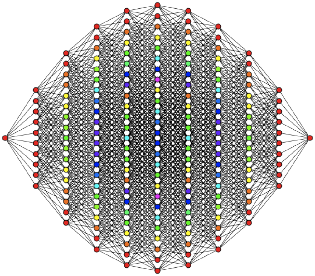
Here is an example where neither Gaussianity, nor hierarchical structure (not even at ”mesoscopic” level, such is the case of the GFF) are available but which still falls in the REM-class. Consider the unit cube in dimensions. To each edge we attach independent exponential random variables with mean one. We write and for diametrically opposite vertices. As an example, the -dimensional hypercube is shown in Figure 3.2 below.
Let now be the set of paths of length from to . Each is of the form . For any such paths, we may consider the sum of edge weights
| (3.19) |
A quantity of interest is the minimal weight when . This is a first passage percolation problem in the ”mean field limit”. To get a feeling of what is going on here, let us consider a reference path and : by Markov inequality (union bound) we have
| (3.20) |
The sum of independent (mean one) exponentials is a well-studied object (one even has a closed form for its distribution - the Erlang distribution); in particular, the following asymptotics is easily checked
| (3.21) |
Using this in (3.20), we see that for . It turns out that this simple ”REM-bound” is tight:
Fact 5.
| (3.22) |
in probability.
The above (3.22) has been conjectured by Aldous [1], who also suggested that a good way to tackle the problem is by means of non-homogeneous dependent branching processes. The conjecture has been settled by Fill and Pemantle [33], although following a different route (a conditional second moment method with ”variance reduction”). On the other hand, the multiscale refinement of the second moment method discussed above seems to be particularly suited to carry out Aldous’ original strategy [3].
Chapter 4 How to identify scales?
4.1 Musing on the Riemann -function
Fyodorov, Keating and Hiary [28] have recently put forward the conjecture that the mechanism underlying the extremes of the hierarchical field might also be found in certain number-theoretical issues, such as the statistics of the extremes of the Riemann -function along the critical line. The latter is of course the function
| (4.1) |
According the Riemann Hypothesis, the zeros of this function lie on the critical line . In general, many questions in the theory of the -function concern the distribution of values on the critical line. A theorem of Selberg [42] states that
| (4.2) |
In other words,
| (4.3) |
”behaves” as a Gaussian random field (indexed by ). This random field is however correlated. In fact, denoting by the average over an interval such that , it is informally demonstrated in [27] (see [11] for a rigorous proof) that
| (4.4) |
What is important for the discussion here is the logarithmic form of the correlation. The simplest model which displays a logarithmic correlation structure is indeed the hierarchical field (upon identifiying the labels with their binary-expansions). Based on this insight, Fyodorov, Keating and Hiary [28] put forward some intriguing conjectures concerning the high values of the Riemann zeta-function. In particular, they consider
| (4.5) |
and conjecture that, for ,
| (4.6) |
A similar formula but with the factor replaced by would hold if one assumes the
random field to be independent: this is the hierarchical field vs. REM scenario. (Similar conjectures
are also available for the characteristic polynomials of CUE random matrices, see [28].)
4.2 On local projections
It should be clear by now that the point of view discussed in the previous sections relies crucially on the identification of scales for the models at hand. Once these are identified, the (multiscale refinement of the) second moment method is well suited to address the question of the extremes. It goes without saying, different models come with varying degrees of technical difficulties, but certain models seem puzzling already at a conceptual level: where are the scales in the Riemann zeta-function? For the hierarchical field this question is easily answered: thanks to the in-built hierarchical structure, one can even visualize the scales, and it is clear what is meant by, say, ”larger scale”. On a structural level, the situation is also easy for the GFF, thanks to the Markovianity and the self-similarity of the field which lead to the representation (3.4). However, none of these properties are available in the case of the Riemann zeta-function, say. Is there a general recipe which allows us to construct the scales, i.e. an underlying tree-like structure, from first principles? This question should be taken with caution: identifying an underlying tree-structure is the foremost step in the implementation of the Parisi theory [38]. Despite the numerous advances in the field, see e.g. [39, 44], an understanding of this issue is yet nowhere in sight. On the other hand, models in the REM-class undergo what physicists refer to as the REM-freezing transition (a prominent feature is the lack of the so-called chaos in temperature). I will not go into any detail here, but I simply mention this to state the claim that for such models, a general recipe to identify scales might already be hiding in the approach discussed above. In fact, there is compelling evidence that the scales are related to certain local projections. To see this, let us go back to the GREM, namely the model
| (4.7) |
where and , , all independent. Again, we assume the normalization . The covariance of this Gaussian field naturally induces a metric on the configuration space :
| (4.8) |
where is the overlap of two configurations. Since the configuration space is endowed with a geometry (eventually induced by the covariance structure), we may introduce the concept of neighborhood of a configuration. One possible definition is
| (4.9) |
for , and .
As we have seen, a good way to tackle the extremes of GREM is to keep track of first and second level, which we achieved by introducing the counting random variable
| (4.10) |
Of course, knowing the specific representation (4.7) is of help to identify first and second level. In many interesting models, however, the equivalent of (4.7) is lacking, so it would be of interest to have a procedure which generates the levels from ”first principles”. Here is a way which unravels the underlying tree-like structure using only the covariance of the field.
Consider a configuration . The idea is to decompose telescopically
| (4.11) |
where is the sigma-field generated by all random variables which are in the -neighborhood of . Due to the simple covariance structure of the GREM(2), there are only few sensible choices for the ”radius”, namely or . In the case the neighborhood consists of the whole configuration space, so the only non-trivial choice is, in fact, . Let us take a closer look at the conditional expectation: in this case is the -field generated by all random variables for which either , or but . But the random variables and are independent as soon as , so we may completely dismiss the collection, i.e.
| (4.12) |
In other words, we are conditioning on those which share the first index with the reference configuration. Since all involved random variables are Gaussian, conditional expectation are nothing but linear combinations of the random variables upon which one conditions: skipping the tedious calculations, one gets
| (4.13) |
By the law of large numbers, the second term above is, in the large limit, exponentially small, almost surely. Furthermore
| (4.14) |
hence
| (4.15) |
where is an exponentially small term, and consequently
| (4.16) |
By locally projecting the field onto a neighborhood measured w.r.t. the metric
induced by the covariance, we have thus constructed first and second level of the tree (up to errors which are completely irrelevant in the large -limit).
Since local projections work smoothly in case of the GREM 11 1 One may follow analogous steps in order to identify the scales in a GREM, for generic . In this case one simply decomposes telescopically into a sum of terms ensuing from local projection on larger and larger neighborhoods. , it is natural to test the method on the GFF. We will see that, indeed, it allows us to generate from first principles the hierarchical decomposition (3.4). To see this, consider the GFF where is a box of size . In this case the overlap of two configurations (sites) is given by
| (4.17) |
where is the Euclidean distance (at least for far enough from the boundary of the box). Let . Implementing the approach through local projections we get the following telescopic decomposition
| (4.18) |
What is the ”neighborhood” in case of the GFF? By (4.17), it holds
| (4.19) |
namely the complement of the Euclidean ball of radius centered in . Denoting by such Euclidean ball, by Markovianity of the GFF we see that conditioning the field upon the complement coincides with conditioning the field on the boundary of . Local projections thus lead to the decomposition
| (4.20) |
for a which may be chosen as we wish. We hardly expect any difference between conditioning upon the sites which are on a (Euclidean) square or on a (Euclidean) ball, so the above representation can be safely identified with (3.3). Iterating the procedure for the second term in the telescopic
decomposition (4.20) (this step is particularly easy here, thanks to the self-similarity of the field) one then immediately obtains (3.4).
Since the procedure identifies from first principles the tree-structure underlying the GREM or that of the GFF, one can only wonder if local projections capture some fundamental aspects lying underneath the surface of models in the REM-class. A natural ”playground” would be of course the case of the Riemann -function, or the characteristic polynomials of CUE random matrices [28, 27]. On a more spin glass side, it would be interesting to see if the local projections allow to identify the scales behind the Parisi landscape in finite-dimensional Euclidean spaces which have been introduced in [26]. These models have been rigorously analyzed in [34] by means of Guerra’s interpolation scheme [32]
and by [5] by means of the Ghirlanda-Guerra identities [30], which are to these days among the most powerful yet mysterious tools in spin glasses. It would be interesting to have a complementary, more transparent approach.
Let me conclude with a caveat. The local projections discussed above should not be understood as a ”frontal attack” to models in the REM-class. In fact, the procedure involves conditional expectations: these are particularly easy to handle if the underlying random variables are Gaussian, but they quickly become demanding/untractable otherwise. This is however a technical difficulty, as opposed to the more structural quest of bringing to the surface ”hidden geometries”. It is the emerging geometrical picture, and perhaps only this, which might be a good starting point for the analysis.
References
- [1] D. Aldous, Probability Approximations via the Poisson Clumping Heuristic, Springer-Verlag (1989)
- [2] N. Alon and J. Spencer, The probabilistic method, Second edition, Wiley-Interscience New York (2000)
- [3] L.-P. Arguin, N. Kistler, and O. Zindy, Percolation on the hypercube, in preparation
- [4] L.-P. Arguin, A. Bovier, and N. Kistler, Genealogy of extremal particles in branching Brownian motion, Comm. Pure and Appl. Math. 64,1647-1676 (2011)
- [5] L.-P. Arguin and O. Zindy, Poisson-Dirichlet statistics for the extremes of a log-correlated Gaussian field, Ann. Appl. Probab. 24, 1446–1481 (2014)
- [6] J.D. Biggins, Martingale convergence in the branching random walk. J. Appl. Probab. 14, 25-37 (1977)
- [7] D. Belius and N. Kistler, The subleading order of two-dimensional cover times, ArXiv e-prints (2014)
- [8] E. Bolthausen and N. Kistler, On a nonhierarchical version of the generalized random energy model. II. Ultrametricity, Stochastic Process. Appl. 119 , 2357-2386 (2009)
- [9] E. Bolthausen and A.-S. Sznitman, Ten Lectures on Random Media, DMV Seminar Band 32, Oberwolfach Lecture Series, Birkhäuser Verlag (2002)
- [10] E. Bolthausen, J.-D. Deuschel, and G. Giacomin, Entropic repulsion and the maximum of the two-dimensional harmonic crystal, Ann. Probab. 29, 1670-1692 (2001)
- [11] P. Bourgade, Mesoscopic fluctuations of the -zeros, Probab. Theor. Rel. Fields 148, 479-500 (2010)
- [12] A. Bovier, From spin glasses to branching Brownian motion – and back?, Proceedings of the 2013 Prague Summer School on Math. Stat. Phys., M. Biskup, J. Cerny, R. Kotecky, eds. , to appear
- [13] A. Bovier and L. Hartung, The extremal process of two-speed branching Brownian motion, Elect. J. Probab. 18, 1-28 (2014)
- [14] A. Bovier and L. Hartung, Variable speed branching Brownian motion 1. Extremal processes in the weak correlation regime, ArXiv e-prints (2014)
- [15] A. Bovier and I. Kurkova, Derrida’s generalized random energy models. 1. Models with finitely many hierarchies. Ann. Inst. H. Poincare. (B) Prob. Stat. 40, 439-480 (2004)
- [16] A. Bovier, I. Kurkova. Derrida’s generalized random energy models. 2. Models with continuous hierarchies. Ann. Inst. H. Poincare. Prob. et Statistiques (B) Prob. Stat. 40, 481-495 (2004)
- [17] A. Bovier and I. Kurkova, A short course on mean field spin glasses, In: A. Boutet de Monvel and A. Bovier (Eds.) Spin Glasses: Statics and Dynamics. Summer School Paris, 2007. Birkhäuser, Basel-Boston-Berlin (2009)
- [18] M. Bramson, Maximal displacement of branching Brownian motion, Comm. Pure and Appl. Math. 31, 531-581 (1978)
- [19] J. Cook, B. Derrida, Finite size effects in random energy models and in the problem of polymers in a random medium, J. Stat. Phys. 63, 505-539 (1991)
- [20] O. Daviaud, Extremes of the discrete two-dimensional Gaussian free field, Ann. Probab. 34, 962-986 (2006)
- [21] A. Dembo, J. Rosen, Y. Peres and O. Zeitouni, Cover times for Brownian motion and random walks in two dimensions, Ann. of Math. (2) 160, 433-464 (2004)
- [22] B. Derrida, Random Energy Model: An exactly solvable model of disordered systems, Phys. Rev. B 24 (1981)
- [23] B. Derrida, A generalization of the random energy model that includes correlations between the energies, J.Phys.Lett. 46, 401-407 (1985)
- [24] M. Fang and O. Zeitouni, Slowdown for time inhomogeneous branching Brownian motion, J. Stat. Phys. 149, 1-9 (2012)
- [25] K. Ford, Sharp probability estimates for random walks with barriers, Probab. Theor. Rel. Fields 145, 269-283 (2009)
- [26] Yan V. Fyodorov and J.-P. Bouchaud Statistical mechanics of a single particle in a multiscale random potential: Parisi landscapes in finite-dimensional Euclidean spaces, J. Phys. A: Math. Theor. 41 324009 (2008)
- [27] Y. V. Fyodorov, and J.P. Keating, Freezing Transitions and Extreme Values: Random Matrix Theory, , and Disordered Landscapes, Phil. Trans. R. Soc. A, in press (2014)
- [28] Y. V. Fyodorov, J.P. Keating, and G.A. Hiary, Freezing transition, characteristic polynomials of random matrices, and the Riemann zeta-function, Phys. Rev. Lett 108 Art. no. 170601 (2012)
- [29] Y. V. Fyodorov, P. Le Doussal, and A. Rosso, Counting function fluctuations and extreme value threshold in multifractal patterns: the case study of an ideal noise, J. Stat. Phys. 149, 898-920 (2012)
- [30] S. Ghirlanda F. Guerra, General properties of overlap probability distributions in disordered spin systems. Towards Parisi ultrametricity, Journal of Physics A: 31.46 (1998)
- [31] J.-B. Gouéré, Branching brownian motion seen from its left-most particle, Bourbaki Seminar 65, n. 1067, SMF (2013)
- [32] F. Guerra, Broken replica symmetry bounds in the mean field spin glass model, Comm. Math. Physics, Vol. 233, 1-12 (2003)
- [33] J. Fill and R. Pemantle, Oriented percolation, first-passage percolation and covering times for Richardson’s model on the n-cube. Ann. Appl. Prob., 3, 593-629 (1993)
- [34] A. Klimovsky, High-dimensional Gaussian fields with isotropic increments seen through spin glasses, Electron. Commun. Probab. 17, 1-14 (2012)
- [35] J. Komlos, P. Major, G. and Tusnady, G. An approximation of partial sums of independent random variables and the sample distribution function, Wahrsch. verw. Gebiete 32, 111-131 (1975)
- [36] P. Maillard and O. Zeitouni, Slowdown in branching Brownian motion with inhomogeneous variance, ArXiv e-prints (2013)
- [37] B. Mallein, Maximal displacement of a branching random walk in time-inhomogeneous environment. ArXiv e-prints (2013)
- [38] M. Mézard, G. Parisi, and M. Virasoro, Spin Glass theory and beyond, World scientific, Singapore (1987)
- [39] D. Panchenko, The Parisi ultrametricity conjecture, Ann. of Math. 177 (1), 383-393 (2013)
- [40] D. Ruelle, A mathematical reformulation of REM and GREM, Comm. Math. Physics, Vol. 108, 225-239 (1987)
- [41] M. Schmidt, PhD Thesis, Frankfurt University (ongoing)
- [42] A. Selberg, Contribution to the theory of the Riemann zeta-function, Arch. Math. Naturvid. 48, pp. 89-155 (1946)
- [43] B. Simon, A celebration of Jürg and Tom, J. Statist. Phys. 134, 809-812 (2009)
- [44] M. Talagrand, Mean field models for spin glasses. I& II, Ergebnisse der Mathematik und ihrer Grenzgebiete, Springer-Verlag Berlin (2011)
- [45] O. Zeitouni, Branching random walks and Gaussian fields, available at http://www.wisdom.weizmann.ac.il/zeitouni/pdf/notesBRW.pdf
N. KISTLER, Institut für Mathematik, Goethe-Universität Frankfurt, DE-60054 Frankfurt am Main, kistler@math.uni-frankfurt.de