跳到论文正文
W Papers独立论文阅读器 arXiv:1412.0893 论文正文 计算阅读时间 · 0%
引用这篇论文根据当前论文元数据生成,正式投稿前建议核对。


License: arXiv.org perpetual non-exclusive license
arXiv:1412.0893v1 [hep-ph] 02 Dec 2014

Large 𝐛\mathbf{b} behaviour in the CGC/saturation approach: BFKL equation with pion loops

Eugene Levin Email: leving@post.tau.ac.il, eugeny.levin@usm.cl Affiliation:  Department of Particle Physics, School of Physics and Astronomy, Tel Aviv University, Tel Aviv, 69978, Israel Affiliation:  Departamento de Física, Universidad Te´\acute{e}cnica Federico Santa María and Centro Científico-Tecnolo´\acute{o}gico de Valparaíso, Casilla 110-V, Valparaiso, Chile
August 24, 2026
Abstract

In this paper we proposed a solution to the longstanding problem of the CGC/saturation approach: the power-like fall of the scattering amplitudes at large bb. This decrease leads to the violation of the Froissart theorem and makes the approach theoretically inconsistent. We showed in the paper that sum of the pion loops results in the exponential fall of the scattering amplitude at large impact parameters and in the restoration of the Froissart theorem.

pacs
25.75.Bh, 13.87.Fh, 12.38.Mh

I Introduction

It is well known that perturbative QCD suffers fundamental problem: the scattering amplitude falls down at large impact parameters (bb) as a power of bb. In particular the CGC/saturation approach[1], which is based on perturbative QCD, faces this problem. Such a power-like decrease leads to the violation[2, 3] of the Froissart theorem[4]. The violation of the Froissart theorem stems from the growth of the radius of interaction as a power of the energy; and can be fixed by introducing a new dimensional scale in addition to the saturation momentum. Since even a power-like decrease provides the small values of the amplitudes at large bb , in the framework of the CGC/saturation approach we need to fix the large bb behaviour in the BFKL evolution equation[5, 6]. Therefore, we have to introduce two dimensional scales in the CGC/saturation approach: the saturation momentum, that is originated by the interactions of the BFKL Pomerons; and the new scale of the non-perturbative source that provides the exponential decrease of the BFKL Pomeron at large bb.

The problem of large bb behaviour of the BFKL Pomeron has not been solved in spite of the numerous attempts based both on analytical and numerical calculations, to approach it [3, 7, 8, 9, 10, 11, 12, 13, 14, 15, 16, 17]. We need to find the sincere theoretical way to introduce the second dimensional scale. The proof of the Froissart theorem indicates that the exponential fall down at large bb is closely related to the contribution of the exchange of two lightest hadrons: pion, in tt-channel (see Fig. 1).

Refer to caption
Figure 1: The exchange of two pions that gives the main contribution to the large bb behaviour of the scattering amplitude[4].

In this paper we propose the theoretical approach which based on the assumption that the BFKL Pomeron, being perturbative in nature, takes into account rather short distances (say of the order of 1/mG1/m_{G}, where mGm_{G} is the mass of the lightest glueball); and the long distance contribution can be described by the exchange of pions (1/2​μ≫ 1/mG1/2\mu\,\gg\,1/m_{G}, where μ\mu is the pion mass). We modify the BFKL Pomeron by including the pions loops shown in Fig. 2 and show that the resulting Pomeron leads to an exponentially small scattering amplitude at large bb. Such behaviour of the scattering amplitude heals all difficulties of the perturbative approach including the violation of the Froissart theorem.

II The BFKL Pomeron

In this section we are going to describe that main features of the BFKL Pomeron which we will need below. All these features are known and can be found in Refs.[5, 6, 18]. We include them for the sake of completeness and of clarification of notations. Let us consider the scattering amplitude of two dipoles with sizes r1r_{1} and r2r_{2} at high energy ss( Y=ln⁡sY=\ln s). The Green’s function of the BFKL Pomeron to the scattering amplitude at fixed momentum transferred along the Pomeron:QTQ_{T} takes the following form[18]

Im​GI​P​(Y,t=−QT2,r1,r2)=r1​r2​∫ϵ−i​∞ϵ+i​∞d​ω2​π​i​eω​Y​GI​P​(ω,QT,r1,r2)\mbox{Im}\,G_{{I\!\!P}}\left(Y,t=-Q^{2}_{T};r_{1},r_{2}\right)\,\,=\,\,r_{1}\,r_{2}\,\int^{\epsilon+i\infty}_{\epsilon-i\infty}\frac{d\omega}{2\pi i}\,e^{\omega\,Y}\,\,G_{{I\!\!P}}\left(\omega,Q_{T};r_{1},r_{2}\right) (1)

The integration contour is situated to the right of all singularities of GI​PG_{I\!\!P} in ω\omega. Function GI​P​(ω,QT,r1,r2)G_{I\!\!P}\left(\omega,Q_{T};r_{1},r_{2}\right) has been found in Ref.[18] and takes the following form (see Eq.35 in Ref.[18])

GI​P​(ω,QT,r1,r2)|ω→ω0​QT→0=πκ0​{(r1r2)κ0+(r2r1)κ0−  2​(QT2​r1​r2)κ0}G_{I\!\!P}\left(\omega,Q_{T};r_{1},r_{2}\right)\Big|_{\begin{minipage}[42.67912pt]{$\omega\to\omega_{0}\\ Q_{T}\to 0$ }\end{minipage}}\,\,=\,\,\,\frac{\pi}{\kappa_{0}}\Bigg\{\left(\frac{r_{1}}{r_{2}}\right)^{\kappa_{0}}\,\,+\,\,\left(\frac{r_{2}}{r_{1}}\right)^{\kappa_{0}}\,\,-\,\,2\,\left(Q^{2}_{T}\,r_{1}\,r_{2}\right)^{\kappa_{0}}\Bigg\} (2)

where κ0\kappa_{0} is the solution of the following equation

ω= 2​α¯S​(ψ⁡(1)−R​e​ψ​(12−κ0))=ω0+D​κ02+𝒪⁡(κ03)\omega\,=\,2\,\bar{\alpha}_{S}\left(\psi(1)-Re{\,\psi\left(\frac{1}{2}-\kappa_{0}\right)}\right)\,\,=\,\,\omega_{0}\,\,+\,\,D\,\kappa^{2}_{0}\,\,+\,\,{\cal O}\left(\kappa_{0}^{3}\right) (3)

and it is equal to

κ0=(ω−ω0)Dwith​ω0=α¯s​4​ln⁡2​and​D=α¯s​14​ζ​(3)\kappa_{0}\,\,=\,\,\sqrt{\frac{\left(\omega\,\,-\,\,\omega_{0}\right)}{D}}~~~~~~\mbox{with}~~~\omega_{0}\,=\,\bar{\alpha}_{s}4\ln 2~~\mbox{and}~~D\,=\,\bar{\alpha}_{s}14\zeta\left(3\right) (4)

From Eq. (2) one can see that in the kinematic region of small QTQ_{T} where |(ω−ω0)​ln2⁡(QT2​r1​r2)|≫ 1|(\omega-\omega_{0})\,\ln^{2}\left(Q^{2}_{T}r_{1}r_{2}\right)|\,\gg\,1 GI​P​(ω,QT,r1,r2)→  1/ω−ω0G_{I\!\!P}\left(\omega,Q_{T};r_{1},r_{2}\right)\,\,\to\,\,1/\sqrt{\omega-\omega_{0}} while ion the region of |(ω−ω0)​ln2⁡(QT2​r1​r2)|∼ 1|(\omega-\omega_{0})\,\ln^{2}\left(Q^{2}_{T}r_{1}r_{2}\right)|\,\sim\,1 GI​PG_{I\!\!P} is less singular (GI​P​(ω,QT,r1,r2)→ω−ω0G_{I\!\!P}\left(\omega,Q_{T};r_{1},r_{2}\right)\,\,\to\,\,\sqrt{\omega-\omega_{0}}.

Refer to caption
Figure 2: The diagrams that describe the pion loop contribution to the BFKL Pomeron. The wavy line describe the BFKL Pomeron, the dashed line stands for pion. The zigzag line denotes the resulting Pomeron.

The scattering amplitude is equal to

A⁡(Y,QT)=∫d2​r1′​∫d2​r2′​|Ψ⁡(r1′)|2​|Ψ⁡(r2′)|2​Im​GI​P​(Y,t=−QT2,r1′,r2′)A\left(Y,Q_{T}\right)\,\,=\,\,\int d^{2}r^{\prime}_{1}\,\int d^{2}r^{\prime}_{2}\,\,|\Psi\left(r^{\prime}_{1}\right)|^{2}\,|\Psi\left(r^{\prime}_{2}\right)|^{2}\,\mbox{Im}\,G_{{I\!\!P}}\left(Y,t=-Q^{2}_{T};r^{\prime}_{1},r^{\prime}_{2}\right) (5)

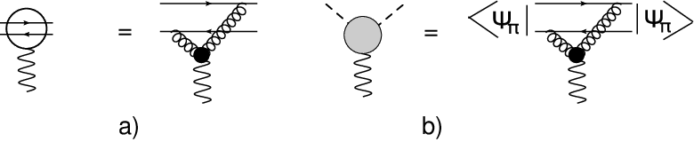
where Ψ\Psi denotes the wave function of the scattering particle (dipole). For the scattering of two dipoles with the sizes r1r_{1} and r2r_{2} |Ψd​i​p​(r1′)|2|\Psi_{dip}\left(r^{\prime}_{1}\right)|^{2} takes the form |Ψd​i​p(r1′)|2=2α¯sδ(r→−r→′)|\Psi_{dip}\left(r^{\prime}_{1}\right)|^{2}=2\bar{\alpha}_{s}\delta\left(\vec{r}-\vec{r}^{\,{}^{\prime}}\right) (see Fig. 3-a). For the scattering of pion Ψπ​(r1)\Psi_{\pi}\left(r_{1}\right) is the non-perturbative wave function of the π\pi-meson (see Fig. 3-b).

Refer to caption
Figure 3: The graphic illustration of Eq. (5): for dipole-Pomeron vertex (Fig. 3-a ) and for the vertex of the interaction of the BFKL Pomeron with a pion (Fig. 3-b).

III Summing pion loops

III.1 General solution

The variables ω\omega and QTQ_{T} are convenient to sum diagrams of Fig. 2 since both variables are preserve along the diagrams of Fig. 2. Indeed, the summation of these diagrams can be done easily (see Fig. 4). The equation that sums the diagrams of Fig. 4-a can be written in the following analytical form:

𝐆I​P​(ω,QT,Rπ,Rπ)=GI​P​(ω,QT,Rπ,Rπ)+GI​P​(ω,QT,Rπ,Rπ)​Σ​(ω,QT)​𝐆I​P​(ω,QT,Rπ,Rπ)\mathbf{G}_{I\!\!P}\left(\omega,Q_{T};R_{\pi},R_{\pi}\right)\,\,=\,\,G_{I\!\!P}\left(\omega,Q_{T};R_{\pi},R_{\pi}\right)\,\,\,+\,\,G_{I\!\!P}\left(\omega,Q_{T};R_{\pi},R_{\pi}\right)\,\Sigma\left(\omega,Q_{T}\right)\mathbf{G}_{I\!\!P}\left(\omega,Q_{T};R_{\pi},R_{\pi}\right) (6)

where 𝐆I​P\mathbf{G}_{I\!\!P} denotes the resulting Green’s function of the Pomeron with the pion loops for r1=r2=Rπr_{1}=r_{2}=R_{\pi} where RπR_{\pi} is the size of the pion. In other words , it is typical size of the integral of Eq. (5) for pion scattering (see Fig. 3-b).

Solution to Eq. (6) takes the form

𝐆I​P​(ω,QT,Rπ,Rπ)=1GI​P−1​(ω,QT,Rπ,Rπ)−Σ⁡(ω,QT)\mathbf{G}_{I\!\!P}\left(\omega,Q_{T};R_{\pi},R_{\pi}\right)\,\,=\,\,\frac{1}{G^{-1}_{I\!\!P}\left(\omega,Q_{T};R_{\pi},R_{\pi}\right)\,\,-\,\,\Sigma\left(\omega,Q_{T}\right)} (7)
Refer to caption
Figure 4: The diagrams of Fig. 2 in ω\omega-representation (Fig. 4-a) and the graphic form of the equation that sums these diagrams (Fig. 4-a)

We use the tt-channel unitarity for 𝐆I​P​(ω,QT,Rπ,Rπ)\mathbf{G}_{I\!\!P}\left(\omega,Q_{T};R_{\pi},R_{\pi}\right) to calculate Σ\Sigma, as it was suggested in Ref.[19]. The unitarity constraints for 𝐆I​P\mathbf{G}_{I\!\!P} takes the form [20, 21] (t=−QT2t=-Q^{2}_{T}):

−i⁡{𝐆I​P​(ω,t+i​ϵ,Rπ,Rπ)−𝐆I​P​(ω,t−i​ϵ,Rπ,Rπ)}=ρ⁡(ω,t)​𝐆I​P​(ω,t+i​ϵ,Rπ,Rπ)​𝐆I​P​(ω,t−i​ϵ,Rπ,Rπ)-i\{\mathbf{G}_{I\!\!P}\left(\omega,t+i\epsilon;R_{\pi},R_{\pi}\right)\,\,-\,\,\mathbf{G}_{I\!\!P}\left(\omega,t-i\epsilon;R_{\pi},R_{\pi}\right)\}\,\,=\,\,\rho\left(\omega,t\right)\mathbf{G}_{I\!\!P}\left(\omega,t+i\epsilon;R_{\pi},R_{\pi}\right)\,\mathbf{G}_{I\!\!P}\left(\omega,t-i\epsilon;R_{\pi},R_{\pi}\right) (8)

Eq. (8) is written for t> 4​μ2t\,>\,4\mu^{2} where μ\mu is the mass of pion. We wish to sum only two pions contribution assuming that all other can be included and have been taken into account in the BFKL Pomeron. Therefore, we believe that Eq. (8) can be trusted for t<mG2t\,<\,m^{2}_{G} where mGm_{G} is the lightest glueball. ρ⁡(ω,t)\rho\left(\omega,t\right) is equal to (t−4​μ2)32+ω/t(t-4\mu^{2})^{\frac{3}{2}+\omega}/\sqrt{t}.

III.2 𝚺\mathbf{\Sigma}

Plugging in Eq. (8) the solution of Eq. (7) one can see that we obtain the following equation for Σ\Sigma:

Imt​Σ​(ω,t)=12​ρ​(ω,t)​(Γπ​πI​P)2​1ω+2\mbox{Im}_{t}\Sigma\left(\omega,t\right)\,\,=\,\,\frac{1}{2}\rho\left(\omega,t\right)\,\Big(\Gamma^{I\!\!P}_{\pi\pi}\Big)^{2}\,\frac{1}{\omega+2} (9)

where vertex Γπ​πI​P\Gamma^{I\!\!P}_{\pi\pi} describes the interaction of the BFKL Pomeron with π\pi-meson (see Fig. 3-b) and takes the simple form (see Eq. (5) and Fig. 3-b). Factor 1/(ω+2)1/(\omega+2) arises in the angular momentum representation from the behaviour of the scattering amplitude due to exchange of two pions as 1/s1/s,

Γπ​πI​P=89​α¯s​∫d2​r​r​|Ψπ​(r)|2=89​α¯s​Rπ\Gamma^{I\!\!P}_{\pi\pi}\,\,=\,\,\frac{8}{9}\bar{\alpha}_{s}\int d^{2}r\,r\,|\Psi_{\pi}\left(r\right)|^{2}\,\,=\,\,\frac{8}{9}\,\bar{\alpha}_{s}\,R_{\pi} (10)

Factor 8/98/9 includes the colour factor and sum of two diagrams in Fig. 3-b.

Experimentally <Rπ2>=0.438±0.008​f​m2<R^{2}_{\pi}>=0.438\pm 0.008\,fm^{2} [23] and this value we will bear in mind for the numerical estimates.

We use the dispersion relations to calculate Σ\Sigma. Since we believe that non-perturbative corrections will not change the intercept of the BFKL Pomeron (see Refs.[16, 17]) we write the dispersion relation with one subtraction. It takes the form

Σ⁡(ω,t)=t​1π​∫d​t′​Imt​Σ​(ω,t′)t′​(t′−t)=t​32​1ω+2​(Γπ​πI​P)2π​∫4​μ2mG2d​t′​ρ​(ω,t′)t′​(t′−t)=α¯s2​169​Rπ2​1ω+2​t​∫4​μ2mG2d​t′​ρ​(ω,t′)t′​(t′−t)\Sigma\left(\omega,t\right)\,\,=\,\,t\,\frac{1}{\pi}\int\frac{dt^{\prime}\,\mbox{Im}_{t}\Sigma\left(\omega,t^{\prime}\right)}{t^{\prime}\,(t^{\prime}-t)}\,\,=\,\,t\frac{3}{2}\,\frac{1}{\omega+2}\frac{\left(\Gamma^{I\!\!P}_{\pi\pi}\right)^{2}}{\pi}\int_{4\mu^{2}}^{m_{G}^{2}}\frac{dt^{\prime}\,\rho\left(\omega,t^{\prime}\right)}{t^{\prime}\,(t^{\prime}-t)}\,\,=\,\,\bar{\alpha}_{s}^{2}\,\frac{16}{9}\,R^{2}_{\pi}\,\,\frac{1}{\omega+2}\,\,t\int_{4\mu^{2}}^{m_{G}^{2}}\,\frac{dt^{\prime}\,\rho\left(\omega,t^{\prime}\right)}{t^{\prime}\,(t^{\prime}-t)} (11)

Factor 3/23/2 stems from two states in tt-channel: π+​π−\pi^{+}\,\pi^{-} and π0​π0\pi^{0}\,\pi^{0}.

The integral over t′t^{\prime} is divergent even after one subtraction. We evaluate this integral making the physical assumption that Imt​Σ​(ω,t′)\mbox{Im}_{t}\Sigma\left(\omega,t^{\prime}\right) is small for t′>mG2t^{\prime}>m^{2}_{G} since all singularities for larger t′t^{\prime} has been taken into account in the BFKL Pomeron contribution. The integral over t′t^{\prime} for ω≪ 1\omega\,\ll\,1 has been taken in Ref.[19]. For fixed ω\omega

Σ⁡(ω,QT)=α¯s2​169​Rπ2​1ω+2​(−QT2)​(mG2)5/2+ω8​μ2∗(5+2​ω)​(4​μ2+QT2)​F1​(52+ω,32,1,72+ω,−mG24​μ2,−mG24​μ2+QT2)\Sigma\left(\omega,Q_{T}\right)\,\,\,=\,\,\,\bar{\alpha}_{s}^{2}\,\frac{16}{9}\,R^{2}_{\pi}\,\,\frac{1}{\omega+2}\,\,(-Q^{2}_{T})\,\frac{\left(m^{2}_{G}\right)^{5/2+\omega}}{8\mu^{2}*\left(5+2\omega\right)\left(4\mu^{2}+Q^{2}_{T}\right)}\,F_{1}\left(\frac{5}{2}+\omega,\frac{3}{2},1,\frac{7}{2}+\omega,-\frac{m^{2}_{G}}{4\mu^{2}},-\frac{m^{2}_{G}}{4\mu^{2}+Q^{2}_{T}}\right) (12)

where F1F_{1} is the Appell F1F_{1} function ( see Ref.[22] formulae 9.180 - 9.184).

The linear term in QT2Q^{2}_{T} can be easily found since two arguments in F1F_{1} coincide and we can use the relation (see Ref.[22] formula 9.182(11)) and reduce Eq. (12) to the form

Σ⁡(ω,QT)=α¯s2​169​Rπ2​1ω+2​(−QT2)​(mG2)5/2+ω8​μ2∗(5+2​ω)​(4​μ2+QT2)​F12​(52+ω,52,72+ω,−mG24​μ2)\Sigma\left(\omega,Q_{T}\right)\,\,\,=\,\,\,\bar{\alpha}_{s}^{2}\,\frac{16}{9}\,R^{2}_{\pi}\,\,\frac{1}{\omega+2}\,\,(-Q^{2}_{T})\,\frac{\left(m^{2}_{G}\right)^{5/2+\omega}}{8\mu^{2}*\left(5+2\omega\right)\left(4\mu^{2}+Q^{2}_{T}\right)}\,{}_{2}F_{1}\left(\frac{5}{2}+\omega,\frac{5}{2},\frac{7}{2}+\omega,-\frac{m^{2}_{G}}{4\mu^{2}}\right) (13)

For mg≫μm_{g}\,\gg\,\mu Eq. (13) takes the form

Σ⁡(ω,QT)\displaystyle\Sigma\left(\omega,Q_{T}\right) =\displaystyle= α¯s2​169​Rπ2​1ω+2​(−QT2)\displaystyle\,\,\,\bar{\alpha}_{s}^{2}\,\frac{16}{9}\,R^{2}_{\pi}\,\,\frac{1}{\omega+2}\,\,(-Q^{2}_{T}) (14)
×\displaystyle\times {1π​ 3​(5+2​ω)​41+ω​(1μ2)12+ω​μ​(2+3​ω+ω3)​Γ​(−2−ω)​Γ​(72+ω)+(mG2)ωω​4+2​ω+3​ω2+ω34​(2+ω)}\displaystyle\Bigg\{\frac{1}{\sqrt{\pi}\,3\left(5+2\omega\right)}4^{1+\omega}\left(\frac{1}{\mu^{2}}\right)^{\frac{1}{2}+\omega}\!\!\!\!\!\!\mu\,\left(2+3\omega+\omega^{3}\right)\Gamma\left(-2-\omega\right)\Gamma\left(\frac{7}{2}+\omega\right)\,+\,\frac{\left(m^{2}_{G}\right)^{\omega}}{\omega}\,\frac{4+2\omega+3\omega^{2}+\omega^{3}}{4(2+\omega)}\Bigg\}
=\displaystyle= −QT2​αe​f​f′​(α¯s)\displaystyle-Q^{2}_{T}\,\alpha^{\prime}_{eff}\left(\bar{\alpha}_{s}\right)

We evaluate αe​f​f′​(α¯s)\alpha^{\prime}_{eff}\left(\bar{\alpha}_{s}\right) using Rπ2=0.436​f​m2R^{2}_{\pi}=0.436fm^{2} and the value for mG2=5​G​e​V2m^{2}_{G}=5\,GeV^{2} that stems from lattice calculation of the glueball masses [24] for the Pomeron trajectory. αe​f​f′​(α¯s)\alpha^{\prime}_{eff}\left(\bar{\alpha}_{s}\right) is shown in Fig. 5. In principle we can consider this coefficient as the only non-perturbative input that we need, but it is pleasant to realize that simple estimates give a sizable value.

Refer to caption
Figure 5: Function αe​f​f′​(α¯s)\alpha^{\prime}_{eff}\left(\bar{\alpha}_{s}\right) of Eq. (14) versus α¯s\bar{\alpha}_{s}, ω=ω0=4​ln⁡2​α¯s\omega=\omega_{0}=4\ln 2\bar{\alpha}_{s}.

III.3 Impact parameter dependence of the resulting Pomeron Green’s function

Plugging Σ\Sigma from Eq. (14) into Eq. (7) we obtain that

𝐆I​P​(ω,QT,Rπ,Rπ)=π​Dω−ω0+αe​f​f′​π​D​QT2\mathbf{G}_{I\!\!P}\left(\omega,Q_{T};R_{\pi},R_{\pi}\right)\,\,=\,\,\frac{\pi\sqrt{D}}{\sqrt{\omega\,-\,\omega_{0}}\,\,+\,\,\alpha^{\prime}_{eff}\pi\sqrt{D}\,Q^{2}_{T}} (15)

Calculating Im​GI​P​(Y,t=−QT2,r1,r2)\mbox{Im}\,G_{{I\!\!P}}\left(Y,t=-Q^{2}_{T};r_{1},r_{2}\right) we substitute Eq. (15) into Eq. (1) and obtain the following equation

Im​GI​P​(Y,QT,Rπ,Rπ)=Rπ2​∫Cd​ω2​π​i​eω​Y​GI​P​(ω,QT,Rπ,Rπ)=∫Cd​δ​ω2​π​i​eω0​Y​eδ​ω​Y​π​D​Rπ2δ​ω+αe​f​f′​π​D​QT2\mbox{Im}\,G_{{I\!\!P}}\left(Y,Q_{T};R_{\pi},R_{\pi}\right)=R^{2}_{\pi}\int_{C}\frac{d\omega}{2\pi i}\,e^{\omega\,Y}\,\,G_{{I\!\!P}}\left(\omega,Q_{T};R_{\pi},R_{\pi}\right)=\int_{C}\!\frac{d\,\delta\omega}{2\pi i}\,e^{\omega_{0}\,Y}\,e^{\delta\omega\,Y}\frac{\pi\sqrt{D}R^{2}_{\pi}}{\sqrt{\delta\omega}\,\,+\,\,\alpha^{\prime}_{eff}\pi\sqrt{D}\,Q^{2}_{T}} (16)

where δ​ω=ω−ω0\delta\omega=\omega\,-\,\omega_{0}.

Refer to caption
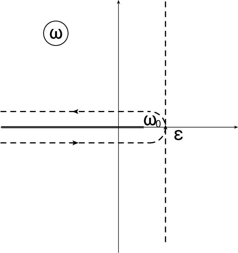
Figure 6: The contour of integration over ω\omega in Eq. (16).

In the impact parameter representation Eq. (16) takes the form

Im​GI​P​(Y,b,Rπ,Rπ)\displaystyle\mbox{Im}\,G_{{I\!\!P}}\left(Y,b;R_{\pi},R_{\pi}\right) =\displaystyle= 2​π​Rπ2​∫0∞QT​d​QT​J0​(QT​b)​∫Cd​δ​ω2​π​i​eω0​Y​eδ​ω​Y​π​Dω−ω0+αe​f​f′​π​D​QT2\displaystyle 2\pi\,R^{2}_{\pi}\,\int^{\infty}_{0}Q_{T}dQ_{T}J_{0}\left(Q_{T}b\right)\int_{C}\!\frac{d\,\delta\omega}{2\pi i}\,e^{\omega_{0}\,Y}\,e^{\delta\omega\,Y}\frac{\pi\sqrt{D}}{\sqrt{\omega\,-\,\omega_{0}}\,\,+\,\,\alpha^{\prime}_{eff}\pi\sqrt{D}\,Q^{2}_{T}} (17)
=\displaystyle= 2​π​Rπ2αe​f​f′​∫Cδ​ω​eω0​Y​eδ​ω​Y​K0​(δ​ωαe​f​f′​D​π​b)\displaystyle\frac{2\pi R^{2}_{\pi}}{\alpha^{\prime}_{eff}}\,\int_{C}\!\!\!\delta\omega\,e^{\omega_{0}\,Y}\,e^{\delta\omega\,Y}\,\,K_{0}\left(\sqrt{\frac{\sqrt{\delta\omega}}{\alpha^{\prime}_{eff}\,D\,\pi}}\,\,b\right)

K0K_{0} in Eq. (17) is modified Bessel function of the second kind (McDonald function) (see Ref.[22] formula 8.43). It is needed in Eq. (17) to take integral over δ​ω\delta\omega which is rather difficult to perform in a general form. However, as we will show below, the extended information on physical observables can be extract from Eq. (17) and Eq. (16) using different asymptotic expantions for which we will be able to take the integral over δ​ω\delta\omega.

IV Physical observables

IV.1 The shrinkage of the diffraction peak.

The diffraction slope BB is defined as

d​σe​ld​QT2=d​σe​ld​QT2|QT=0​e−B​QT2\frac{d\sigma_{el}}{dQ^{2}_{T}}\,\,=\,\,\frac{d\sigma_{el}}{dQ^{2}_{T}}\Big|_{Q_{T}=0}\,e^{-B\,Q^{2}_{T}} (18)

where σe​l\sigma_{el} is the elastic cross section.

Since d​σe​l/d​QT2∝|A|2d\sigma_{el}/dQ^{2}_{T}\propto|A|^{2} where AA is the scattering amplitude, one can see that B=2​d​ln⁡A/d​QT2B\,\,=2d\ln A/dQ^{2}_{T} at QT=0Q_{T}=0. Using Eq. (16) we can calculate the slope: viz.

B\displaystyle B\, =\displaystyle=  2​d​Im​GI​P​(Y,QT,Rπ,Rπ)/d​QT2|QT=0Im​GI​P​(Y,QT,Rπ,Rπ)|QT=0=  2​αe​f​f′​D​π​∫Cd​δ​ω2​π​i​eω0​Y​eδ​ω​Y​π​Dω−ω0∫Cd​δ​ω2​π​i​eω0​Y​eδ​ω​Y​π​Dω−ω0\displaystyle\,2\frac{d\mbox{Im}\,G_{{I\!\!P}}\left(Y,Q_{T};R_{\pi},R_{\pi}\right)\Big/dQ^{2}_{T}|_{Q_{T}=0}}{\mbox{Im}\,G_{{I\!\!P}}\left(Y,Q_{T};R_{\pi},R_{\pi}\right)|_{Q_{T}=0}}\,\,=\,\,2\,\frac{\alpha^{\prime}_{eff}\sqrt{D}\pi\int_{C}\!\frac{d\,\delta\omega}{2\pi i}\,e^{\omega_{0}\,Y}\,e^{\delta\omega\,Y}\frac{\pi\sqrt{D}}{\sqrt{\omega\,-\,\omega_{0}}}}{\int_{C}\!\frac{d\,\delta\omega}{2\pi i}\,e^{\omega_{0}\,Y}\,e^{\delta\omega\,Y}\frac{\pi\sqrt{D}}{\omega\,-\,\omega_{0}}} (19)
=\displaystyle=  2​αe​f​f′​D​Y≡ 2​αe​f​f′​D​ln⁡s\displaystyle\,2\,\alpha^{\prime}_{eff}\,\sqrt{D}\,\sqrt{Y}\,\equiv\,2\,\alpha^{\prime}_{eff}\,\sqrt{D}\,\sqrt{\ln s}

Integrating over δ​ω\delta\omega in Eq. (19) we close contour CC as it is shown in Fig. 6.

B∝ln⁡sB\propto\sqrt{\ln s} is quite different from the Regge behaviour of B∝ln⁡sB\propto\ln s but it has been expected [8]. The slope BB is related to average impact parameter in the interaction B=12​⟨b2⟩B=\frac{1}{2}\langle b^{2}\rangle and its increase with energy occurs due to Gribov’s diffusion in the transverse plane. At each emission the parton changes its position in bb by Δ​b∝1/pT\Delta b\propto 1/p_{T} where pTp_{T} is the transverse momentum of the parton. In the BFKL Pomeron the average transverse momentum increases with energy faster than ln⁡s\ln s . Therefore, Δ​b→0\Delta b\to 0 and we do not see any dependence of ⟨b2⟩\langle b^{2}\rangle with energy for the BFKL Pomeron. Such a dependence is closely related to the confinement of parton in QCD. As it was argued in Ref.[8] if we assume that all transverse momenta of partons due to confinement are larger than some dimensional parameter μ\mu(pT≥μp_{T}\geq\mu), in this case all parton with pT∼μp_{T}\sim\mu can have Gribov’s diffusion with ⟨b2⟩∝1μ2​ln⁡s\langle b^{2}\rangle\propto\frac{1}{\mu^{2}}\,\ln s . However, to calculate the average slope we need to multiply this ⟨b2⟩\langle b^{2}\rangle by the probability to find a parton (P⁡(pT=μ)P(p_{T}=\mu)) with pT∼μp_{T}\sim\mu which is ∝1/ln⁡s\propto 1/\sqrt{\ln s} . Finally B∝P⁡(pT=μ)​1μ2​ln⁡s∝1μ2​ln⁡sB\propto\,P(p_{T}=\mu)\frac{1}{\mu^{2}}\,\ln s\propto\frac{1}{\mu^{2}}\,\sqrt{\ln s}.

Therefore, our approach gives the possibility to incorporate these physical ideas and suggests the theoretical procedure to introduce a new dimensional scale of the non-perturbative origin. It also allows to estimate the value of this scale.

The typical values of QT2Q^{2}_{T} for which we can trust Eq. (18) can be estimated from B​QT2≤ 1B\,Q^{2}_{T}\,\leq\,1 or QT2≤ 1/(2​αe​f​f′​D​ln⁡s)≪ 1/Rπ2Q^{2}_{T}\,\leq\,1/\left(2\,\alpha^{\prime}_{eff}\,\sqrt{D}\,\sqrt{\ln s}\right)\,\,\ll\,1/R^{2}_{\pi}. Such small values of QTQ_{T} justifies the use of Eq. (2) at small QT→0Q_{T}\to 0.

IV.2 Large impact parameter behaviour of the scattering amplitude

We can use the asymptotic behaviour of K0K_{0} at large bb and reduce integral of Eq. (17) to the following expression

Im​GI​P​(Y,b,Rπ,Rπ)→b2≫αe​f​f′2​π​Rπ2αe​f​f′​∫Cδ​ω​eω0​Y​eδ​ω​Y​exp⁡(−δ​ωαe​f​f′​D​π​b)\mbox{Im}\,G_{{I\!\!P}}\left(Y,b;R_{\pi},R_{\pi}\right)\,\,\xrightarrow{b^{2}\gg\alpha^{\prime}_{eff}}\,\,\frac{2\pi\,R^{2}_{\pi}}{\alpha^{\prime}_{eff}}\,\int_{C}\!\!\!\delta\omega\,e^{\omega_{0}\,Y}\,e^{\delta\omega\,Y}\,\,\exp\left(-\sqrt{\frac{\sqrt{\delta\omega}}{\alpha^{\prime}_{eff}\,D\,\pi}}\,\,b\right) (20)

The integral over δ​ω\delta\omega can be taken using the steepest decent method. The equation for the saddle point in δ​ω\delta\omega takes the form

Y−14​((δ​ωS​P)−34​1αe​f​f′​D​π​b)=  0;δ​ωS​P=(b4​αe​f​f′​D​π​Y)43;Y\,-\,\frac{1}{4}\left(\left(\delta\omega_{SP}\right)^{-\frac{3}{4}}\sqrt{\frac{1}{\alpha^{\prime}_{eff}\,D\,\pi}}\,\,\,b\,\,\right)\,\,=\,\,0;~~~~~~~~~~~~~~~\delta\omega_{SP}\,\,=\,\,\left(\frac{b}{4\,\sqrt{\alpha^{\prime}_{eff}\,D\,\pi}\,Y}\right)^{\frac{4}{3}}; (21)

Plugging Eq. (21) in Eq. (20) we obtain that

Im​GI​P​(Y,b,Rπ,Rπ)∝eω0​Y​exp⁡(−3​(b4256​αe​f​f′2​D2​π2​Y)13)\mbox{Im}\,G_{{I\!\!P}}\left(Y,b;R_{\pi},R_{\pi}\right)\,\,\,\propto\,\,\,e^{\omega_{0}\,Y}\,\exp\left(-3\left(\frac{b^{4}}{256\,\alpha^{\prime 2}_{eff}\,D^{2}\,\pi^{2}\,Y}\right)^{\frac{1}{3}}\right) (22)

From Eq. (22) we see that scattering amplitude falls down exponentially. As we will show below such behaviour will restore the Froissart theorem and transforms the CGC/saturation approach into self-consistent effective theory describing QCD at high energies.

IV.3 Restoration of the Froissart theorem

The total cross section σt​o​t\sigma_{tot} in our approach is equal to

σt​o​t,=  2​∫d2​b​Im​A​(s,b)=  2​∫0b0d2​b​Im​A​(s,b)+  2​∫b0∞d2​b​Im​A​(s,b)\sigma_{tot}\\ ,=\,\,2\int d^{2}b\,\mbox{Im}A\left(s,b\right)\,\,=\,\,2\int^{b_{0}}_{0}d^{2}b\,\mbox{Im}A\left(s,b\right)\,\,+\,\,2\int^{\infty}_{b_{0}}d^{2}b\,\mbox{Im}A\left(s,b\right) (23)

Following Ref.[4] we estimate the behaviour of the total cross section dividing the integration over the impact parameter in two parts : b≤b0b\leq b_{0}, where amplitude Im​A​(s,b)≤ 1\mbox{Im}A\left(s,b\right)\,\leq\,1 due to ss-channel unitarity ; and b≥b0b\geq b_{0} where Im​A​(s,b)≪1\mbox{Im}A\left(s,b\right)\ll 1. The value of b0b_{0} can be estimated from the condition that Im​A​(s,b)=f≪ 1\mbox{Im}A\left(s,b\right)\,=\,f\,\ll\,1. In our approach this condition can be re-written, using Eq. (22), as follow

Im​A​(s,b)∝Im​GI​P​(Y,b,Rπ,Rπ)→b2≫αe​f​f′eω0​Y​exp⁡(−3​(b4256​αe​f​f′2​D2​π2​Y)13)=f\mbox{Im}A\left(s,b\right)\,\propto\,\mbox{Im}\,G_{{I\!\!P}}\left(Y,b;R_{\pi},R_{\pi}\right)\,\xrightarrow{b^{2}\gg\,\alpha^{\prime}_{eff}}\,e^{\omega_{0}\,Y}\,\exp\left(-3\left(\frac{b^{4}}{256\,\alpha^{\prime 2}_{eff}\,D^{2}\,\pi^{2}\,Y}\right)^{\frac{1}{3}}\right)\,\,=\,\,f (24)

Eq. (24) leads to

b0=43​ω04/3​αe​f​f′​D​π​Yb_{0}\,\,=\,\,\frac{4}{3}\omega^{4/3}_{0}\sqrt{\alpha^{\prime}_{eff}\,D\,\pi}\,\,\,Y (25)

Plugging this b0b_{0} into Eq. (23) we obtain

σt​o​t≤  4​π​b02+  4​π​f​16​D​π3​3​(αe​f​f′​b0)2/3∼Y2=ln2⁡s\sigma_{tot}\,\,\leq\,\,4\pi b^{2}_{0}\,\,+\,\,4\,\pi\,f\,\frac{16\,D\,\pi}{3\sqrt{3}}\,\left(\alpha^{\prime}_{eff}\,b_{0}\right)^{2/3}\,\,\sim\,\,Y^{2}=\ln^{2}s (26)

Therefore, we see that the Froissart theorem is correct in our approach.

IV.4 𝐐𝐓\mathbf{Q_{T}} dependece of the scattering amplitude.

Integral over ω\omega in Eq. (16) can be taken if we close contour CC as it is shown in Fig. 6. Eq. (16) takes the form

Im​GI​P​(Y,QT,Rπ,Rπ)=Rπ2​∫Cd​δ​ω2​π​i​eω0​Y​eδ​ω​Y​π​Dδ​ω+αe​f​f′​π​D​QT2=D​Rπ2​eω0​Y​∫0∞d​t​e−t2​Y​t2t2+Q¯T4\displaystyle\mbox{Im}\,G_{{I\!\!P}}\left(Y,Q_{T};R_{\pi},R_{\pi}\right)~=~R^{2}_{\pi}\,\int_{C}\!\frac{d\,\delta\omega}{2\pi i}\,e^{\omega_{0}\,Y}\,e^{\delta\omega\,Y}\frac{\pi\sqrt{D}}{\sqrt{\delta\omega}\,\,+\,\,\alpha^{\prime}_{eff}\pi\sqrt{D}\,Q^{2}_{T}}\,\,=\,\,\sqrt{D}\,R^{2}_{\pi}\,e^{\omega_{0}\,Y}\,\int^{\infty}_{0}dte^{-t^{2}\,Y}\frac{t^{2}}{t^{2}+\bar{Q}^{4}_{T}}\,\,
(t=ω0−ω,Q¯t=αe​f​f′​π​D​QT)=12​D​Q¯T2​Rπ2​eω0​Y​{−ez2+1π​z+ez2​e​r​f​(z)}\displaystyle\left(t=\sqrt{\omega_{0}-\omega},\bar{Q}_{t}\,=\,\sqrt{\alpha^{\prime}_{eff}\pi\sqrt{D}}\,\,Q_{T}\right)~=\,\,\frac{1}{2}\sqrt{D}\bar{Q}^{2}_{T}\,R^{2}_{\pi}\,\,e^{\omega_{0}\,\,Y}\,\,\Bigg\{-e^{z^{2}}+\frac{1}{\sqrt{\pi}z}\,+\,e^{z^{2}}erf(z)\Bigg\} (27)

where z=Q¯T2​Yz=\bar{Q}^{2}_{T}\,\sqrt{Y} and e​r​f​(z)erf(z) is the error function (see function Φ⁡(z)\Phi(z) in Ref.[22], formula 8.25).

Since

{…}⟶{z≪ 1,πz−πz≫ 1,π2​z3\Big\{\dots\Big\}\,\,\longrightarrow\,\,\left\{\begin{array}[]{l l}z\,\ll\,1,&\,\,\,\frac{\pi}{z}\,\,-\,\,\pi\\ &\\ z\,\gg\,1,&\,\,\,\frac{\sqrt{\pi}}{2\,\,z^{3}}\end{array}\right. (28)

one can see that at small values of QTQ_{T} Im​G\mbox{Im}\,G behaves with the slope that has been calculated, and at large QTQ_{T} in falls down as 1/(QT4​Y3/2)1/\left(Q^{4}_{T}\,\,Y^{3/2}\right).

IV.5 Dependence on the sizes of interacting dipoles

We have discussed the Green’s function for the interaction of two dipoles with the same large sizes RπR_{\pi}. Coming back to Eq. (5) one can see that we need actually the Green’s function for different dipole sizes. Let us consider first Im​GI​P​(Y,t=−QT2,r,Rπ)\mbox{Im}\,G_{{I\!\!P}}\left(Y,t=-Q^{2}_{T};r,R_{\pi}\right). The typical processes which can be described by such Green’s function include inclusive deep inelastic scattering as well as diffraction dissociation by the virtual photon. We need to replace one (say, the upper in Fig. 2) BFKL Pomeron Green’s function by GI​P​(ω,QT,r,Rπ)G_{I\!\!P}\left(\omega,Q_{T};r,R_{\pi}\right) which is given by Eq. (2): viz.

GI​P​(ω,QT,r,Rπ)=πκ0​{(Rπr)κ0+(rRπ)κ0−  2​(QT2​r​Rπ)κ0}G_{I\!\!P}\left(\omega,Q_{T};r,R_{\pi}\right)\,\,=\,\ \,\frac{\pi}{\kappa_{0}}\Bigg\{\left(\frac{R_{\pi}}{r}\right)^{\kappa_{0}}\,\,+\,\,\left(\frac{r}{R_{\pi}}\right)^{\kappa_{0}}\,\,-\,\,2\,\left(Q^{2}_{T}\,r\,R_{\pi}\right)^{\kappa_{0}}\Bigg\} (29)

As a result Eq. (16) should be replaced by the following equation

Im​GI​P​(Y,QT,r,Rπ)=r​Rπ​D​∫Cd​δ​ω2​π​i​eω0​Y​eδ​ω​Y​{(Rπr)δ​ω/D+(rRπ)δ​ω/D−  2​(QT2​r​Rπ)δ​ω/D}δ​ω+αe​f​f′​π​D​QT2\mbox{Im}\,G_{{I\!\!P}}\left(Y,Q_{T};r,R_{\pi}\right)\,\,=\,\,r\,R_{\pi}\,\sqrt{D}\,\int_{C}\!\frac{d\,\delta\omega}{2\pi i}\,e^{\omega_{0}\,Y}\,e^{\delta\omega\,Y}\frac{\Big\{\left(\frac{R_{\pi}}{r}\right)^{\sqrt{\delta\omega/D}}\,\,+\,\,\left(\frac{r}{R_{\pi}}\right)^{\sqrt{\delta\omega/D}}\,\,-\,\,2\,\left(Q^{2}_{T}\,r\,R_{\pi}\right)^{\sqrt{\delta\omega/D}}\Big\}}{\sqrt{\delta\omega}\,\,+\,\,\alpha^{\prime}_{eff}\pi\sqrt{D}\,Q^{2}_{T}} (30)

Closing contour CC in the integral over δ​ω\delta\omega as it is shown inFig. 6 and using the same notations as in Eq. (27) we obtain

Im​GI​P​(Y,QT,r,Rπ)=  2​r​Rπ​D​eω0​Y​∫0∞d​t​e−t2​Y\displaystyle\mbox{Im}\,G_{{I\!\!P}}\left(Y,Q_{T};r,R_{\pi}\right)\,\,=\,\,2\,r\,R_{\pi}\,\sqrt{D}\,e^{\omega_{0}\,Y}\,\int^{\infty}_{0}dt\,e^{-t^{2}\,Y} (31)
×{t2t2+Q¯T4​(cos⁡(tD​ln⁡(Rπr))−cos⁡(tD​ln⁡(QT2​r​Rπ)))−t​Q¯T2t2+Q¯T4​sin⁡(tD​ln⁡(QT2​r​Rπ))}\displaystyle\times\,\,\Bigg\{\frac{t^{2}}{t^{2}+\bar{Q}^{4}_{T}}\left(\cos\left(\frac{t}{\sqrt{D}}\,\ln\left(\frac{R_{\pi}}{r}\right)\right)\,\,-\,\,\cos\left(\frac{t}{\sqrt{D}}\,\ln\left(Q^{2}_{T}\,r\,R_{\pi}\right)\right)\right)\,\,-\,\,\frac{t\bar{Q}^{2}_{T}}{t^{2}+\bar{Q}^{4}_{T}}\,\sin\left(\frac{t}{\sqrt{D}}\,\ln\left(Q^{2}_{T}\,r\,R_{\pi}\right)\right)\Bigg\}

IV.5.1 𝐐𝐓\mathbf{Q_{T}} = 0

At QT=0Q_{T}=0 the integral over tt in Eq. (31) can be taken and it leads to

Im​GI​P​(Y,QT,r,Rπ)=  2​r​Rπ​π​D​exp⁡(ω0​Y−ln2⁡(Rπ/r)4​D​Y)​(1+e​r​f​(i​ln⁡(Rπ/r)2​D​Y))2​Y\mbox{Im}\,G_{{I\!\!P}}\left(Y,Q_{T};r,R_{\pi}\right)\,\,=\,\,2\,r\,R_{\pi}\,\sqrt{\pi\,D}\,\exp\left(\omega_{0}\,Y\,\,-\,\,\frac{\ln^{2}\left(R_{\pi}/r\right)}{4\,D\,Y}\right)\,\,\frac{\left(1\,+\,erf\left(i\frac{\ln\left(R_{\pi}/r\right)}{2\sqrt{D\,Y}}\right)\right)}{2\sqrt{Y}} (32)

One can see that for small ln⁡(Rπ/r)2​D​Y≪ 1\frac{\ln\left(R_{\pi}/r\right)}{2\sqrt{D\,Y}}\,\ll\,1 e​r​f​(i​ln⁡(Rπ/r)2​D​Y)erf\left(i\frac{\ln\left(R_{\pi}/r\right)}{2\sqrt{D\,Y}}\right) tends to zero and the integral in Eq. (31) can be calculaterd using the steepest decent method with the saddle point in tS​P=i​ln⁡(Rπ/r)2​D​Yt_{SP}=i\frac{\ln\left(R_{\pi}/r\right)}{2\sqrt{D\,Y}}.

IV.5.2 𝐐𝐓𝟐​𝐫​𝐑π≪  1\mathbf{Q^{2}_{T}\,r\,R_{\pi}}\,\,\ll\,\,1

In this kinematic region we can neglect the last term in Eq. (29). Taking the integral using the steepest decent method we obtain

Im​GI​P​(Y,QT,r,Rπ)\displaystyle\mbox{Im}\,G_{{I\!\!P}}\left(Y,Q_{T};r,R_{\pi}\right)\,\, =\displaystyle=   2​r​Rπ​π​D​exp⁡(ω0​Y−ln2⁡(Rπ/r)4​D​Y)​tS​P2tS​P2+Q¯T4\displaystyle\,\,2\,r\,R_{\pi}\,\sqrt{\pi\,D}\,\exp\left(\omega_{0}\,Y\,\,-\,\,\frac{\ln^{2}\left(R_{\pi}/r\right)}{4\,D\,Y}\right)\,\,\frac{t^{2}_{SP}}{t^{2}_{SP}\,\,+\,\,\bar{Q}_{T}^{4}}\,\, (33)
=\displaystyle=     2​r​Rπ​π​D​exp⁡(ω0​Y−ln2⁡(Rπ/r)4​D​Y)​11−Q¯T4​ 4​D​Y/ln2⁡(Rπ/r)\displaystyle\,\,\,\,2\,r\,R_{\pi}\,\sqrt{\pi\,D}\,\exp\left(\omega_{0}\,Y\,\,-\,\,\frac{\ln^{2}\left(R_{\pi}/r\right)}{4\,D\,Y}\right)\,\,\frac{1}{1-\bar{Q}^{4}_{T}\,4\,D\,Y/\ln^{2}\left(R_{\pi}/r\right)}

We can trust Eq. (33) for QT4≤ln2⁡(Rπ/r)/(4​D​Y)Q^{4}_{T}\,\,\leq\,\,\ln^{2}\left(R_{\pi}/r\right)/\left(4\,D\,Y\right). This inequality specifies the kinematic region in which the pion loops gives an essential contribution.

IV.5.3 𝐐𝐓𝟐​𝐫​𝐑π≥  1\mathbf{Q^{2}_{T}\,r\,R_{\pi}}\,\,\geq\,\,1

In this kinematic region we need to use all three terms of Eq. (29). Using the steepest decent method we obtain

Im​GI​P​(Y,QT,r,Rπ)\displaystyle\mbox{Im}\,G_{{I\!\!P}}\left(Y,Q_{T};r,R_{\pi}\right)\,\, =\displaystyle=   2​r​Rπ​π​D​exp⁡(ω0​Y−ln2⁡(Rπ/r)4​D​Y)​11−Q¯T4​ 4​D​Y/ln2⁡(Rπ/r)\displaystyle\,\,2\,r\,R_{\pi}\,\sqrt{\pi\,D}\,\exp\left(\omega_{0}\,Y\,\,-\,\,\frac{\ln^{2}\left(R_{\pi}/r\right)}{4\,D\,Y}\right)\,\,\frac{1}{1-\bar{Q}^{4}_{T}\,4\,D\,Y/\ln^{2}\left(R_{\pi}/r\right)} (34)
+\displaystyle+   2​r​Rπ​π​D​exp⁡(ω0​Y−ln2⁡(QT2​r​Rπ)4​D​Y)​Q¯T2​ln⁡(QT2​r​Rπ)4​D​Y1−Q¯T4​ 4​D​Y/ln2⁡(QT2​r​Rπ)\displaystyle\,\,2\,r\,R_{\pi}\,\sqrt{\pi\,D}\,\exp\left(\omega_{0}\,Y\,\,-\,\,\frac{\ln^{2}\left(Q^{2}_{T}\,r\,R_{\pi}\right)}{4\,D\,Y}\right)\,\,\frac{\bar{Q}^{2}_{T}\sqrt{\frac{\ln\left(Q^{2}_{T}\,r\,R_{\pi}\right)}{4\,D\,Y}}}{1-\bar{Q}^{4}_{T}\,4\,D\,Y/\ln^{2}\left(Q^{2}_{T}\,r\,R_{\pi}\right)}

IV.5.4 Impact parameter dependence

Using Eq. (30) we can find the Green’s function in bb-representation using the general form of the BFKL Pomeron given by Eq. (29). It takes the form

Im​GI​P​(Y,b,r,Rπ)=2​π​Rπ2αe​f​f′​∫Cδ​ω​eω0​Y​eδ​ω​Y\displaystyle\mbox{Im}\,G_{{I\!\!P}}\left(Y,b;r,R_{\pi}\right)\,\,=\,\,\frac{2\pi R^{2}_{\pi}}{\alpha^{\prime}_{eff}}\,\int_{C}\!\!\!\delta\omega\,e^{\omega_{0}\,Y}\,e^{\delta\omega\,Y}\!\!\!\!\!\! ({(Rπr)δ​ω/D+(rRπ)δ​ω/D}​K0​(δ​ωαe​f​f′​D​π​b)CLOSE\displaystyle\left(\left\{\left(\frac{R_{\pi}}{r}\right)^{\sqrt{\delta\omega/D}}\,\,+\,\,\left(\frac{r}{R_{\pi}}\right)^{\sqrt{\delta\omega/D}}\right\}\,K_{0}\left(\sqrt{\frac{\sqrt{\delta\omega}}{\alpha^{\prime}_{eff}\,D\,\pi}}\,\,b\right)\right. (35)
OPEN− 2​(r​Rπ​δ​ωαe​f​f′​D​π)δ​ω/D​Kδ​ω/D​(δ​ωαe​f​f′​D​π​b))\displaystyle\,\,\left.\,~~~~-\,2\,\,\left(\frac{r\,R_{\pi}\,\sqrt{\delta\omega}}{\alpha^{\prime}_{eff}\,D\,\pi}\right)^{\sqrt{\delta\omega/D}}\,K_{\sqrt{\delta\omega/D}}\left(\sqrt{\frac{\sqrt{\delta\omega}}{\alpha^{\prime}_{eff}\,D\,\pi}}\,\,b\right)\right)

We can single out several kinematic regions where Eq. (35) takes different form:

  1. 1.

    bb is small and Rπ≫ 1R_{\pi}\,\gg\,1. The main contribution stems from the saddle point δ​ωS​P=−ln(Rπ/r)/(2DY)\sqrt{\delta\omega_{SP}}\,=\,-\ln\left(R_{\pi}/r\right)/\left(2\sqrt{D}Y\right) . If r​Rπ​δ​ωS​P≪ 1r\,R_{\pi}\sqrt{\delta\omega_{SP}}\,\ll\,1 we can neglect the second term in Eq. (35) and the amplitude will be equal to Eq. (32) which is multiplied by K0​(δ​ωS​Pαe​f​f′​D​π​b)K_{0}\left(\sqrt{\frac{\sqrt{\delta\omega_{SP}}}{\alpha^{\prime}_{eff}\,D\,\pi}}\,\,b\right). The second term in Eq. (35) can be neglected.

  2. 2.

    bb is small and Rπ≫ 1R_{\pi}\,\gg\,1, but r​Rπ​δ​ωS​P≫ 1r\,R_{\pi}\sqrt{\delta\omega_{SP}}\,\gg\,1. The second term should be taken into account with the saddle point in δ​ωS​P=−ln(Rπr)/(2DY)\sqrt{\delta\omega_{SP}}\,=\,-\ln\left(R_{\pi}\,r\right)/\left(2\sqrt{D}Y\right).

  3. 3.

    bb is large. The both terms can be calculated with the saddle point from Eq. (21) leading to the same behaviour at large bb which is given by the exponent in Eq. (22). The estimates for how large have to be bb, come from the condition δ​ωS​P\delta\omega_{SP} of Eq. (21) is much larger than ln⁡(Rπ/r)/(2​D​Y)\,\ln\left(R_{\pi}/r\right)/\left(2\sqrt{D}Y\right).

We hope that we have demonstrated how the pion loops affect the scattering amplitude, leaving more elaborate calculations to the reader.

IV.6 𝐛\mathbf{b} dependence for general case of two dipoles with different sizes

In this section we consider the large bb behaviour of the Green’s function for the general case of two dipoles with sizes r1r_{1} and r2r_{2}. For such scattering the first diagram in Fig. 2 looks differently than all others and the sum of all diagrams can be written as

G⁡(ω,QT,r1,r2)=\displaystyle G\left(\omega,Q_{T};r_{1},r_{2}\right)\,\,= (36)
GI​P​(ω,QT,r1,r2)+GI​P​(ω,QT,r1,Rπ)​Σ​(ω)​𝐆​(ω,QT,Rπ,Rπ)​GI​P−1​(ω,QT,Rπ,Rπ)​GI​P​(ω,QT,r2,Rπ)\displaystyle G_{I\!\!P}\left(\omega,Q_{T};r_{1},r_{2}\right)\,\,\,+\,\,\,G_{I\!\!P}\left(\omega,Q_{T};r_{1},R_{\pi}\right)\Sigma\left(\omega\right)\mathbf{G}\left(\omega,Q_{T};R_{\pi},R_{\pi}\right)G^{-1}_{I\!\!P}\left(\omega,Q_{T};R_{\pi},R_{\pi}\right)\,G_{I\!\!P}\left(\omega,Q_{T};r_{2},R_{\pi}\right)

As it has been discussed for large impact parameter behaviour we can restrict ourselves by the region of very small QTQ_{T} and neglect the last term in the BFKL Pomeron Green’s function of Eq. (2).

Plugging in Eq. (36) Eq. (2) and Eq. (15) we can re-write Eq. (36) in the form

G⁡(ω,QT,r1,r2)\displaystyle G\left(\omega,Q_{T};r_{1},r_{2}\right)\,\, =\displaystyle= −π​Dω−ω0​{(Rπ2r1​r2)(ω−ω0)/D+(Rπ2r1​r2)−(ω−ω0)/D}\displaystyle\,\,-\frac{\pi\sqrt{D}}{\sqrt{\omega\,-\,\omega_{0}}}\Bigg\{\left(\frac{R^{2}_{\pi}}{r_{1}\,r_{2}}\right)^{\sqrt{(\omega-\omega_{0})/D}}\,+\,\left(\frac{R^{2}_{\pi}}{r_{1}\,r_{2}}\right)^{-\,\sqrt{(\omega-\omega_{0})/D}}\Bigg\} (37)
+\displaystyle+ π​Dω−ω0+αe​f​f′​π​D​QT2​{(r1r2)(ω−ω0)/D+(r1r2)−(ω−ω0)/D}\displaystyle\,\,\frac{\pi\sqrt{D}}{\sqrt{\omega\,-\,\omega_{0}}\,\,+\,\,\alpha^{\prime}_{eff}\pi\sqrt{D}\,Q^{2}_{T}}\Bigg\{\left(\frac{r_{1}}{r_{2}}\right)^{\sqrt{(\omega-\omega_{0})/D}}\,+\,\left(\frac{r_{1}}{r_{2}}\right)^{-\,\sqrt{(\omega-\omega_{0})/D}}\Bigg\}

The last term leads to the exponential fall down at large bb that has been discussed in section IV-B (see Eq. (24) ). The first term does not depend on QTQ_{T} and gives δ⁡(b)\delta\left(b\right) for bb dependence., and, therefore does not contribute in the scattering amplitude at large bb.

V Conclusions

In this paper we proposed a solution to the longstanding problem of the CGC/saturation approach: the power-like fall of the scattering amplitudes at large bb. This decrease leads to the violation of the Froissart theorem and makes the approach theoretically inconsistent. We showed in the paper that sum of the pion loops results in the exponential fall of the scattering amplitude at large impact parameters and in the restoration of the Froissart theorem. Hence we resolve the fundamental difficulty of the CGC/saturation approach.

Our solution is based on the assumption which we have to make in the absence of consistent approach to non-perturbative QCD. We assume that the BFKL Pomeron which stems from perturbative QCD calculations, can be used for the description of the long distance physics but the typical distances in this Pomeron is smaller that 1/mπ1/m_{\pi}. Making this assumption more specific we assume that the BFKL Pomeron, analytically continuated to the tt-channel, has all singularities in the tt-channel at the values of tt which are much larger than 4​mπ24m^{2}_{\pi}. We see support of this assumption in the lattice calculations which show that the Pomeron trajectory[24] has the lightest glueball on it with mG2=5​G​e​V2m^{2}_{G}=5\,GeV^{2}.

Our summation procedure preserves the spectrum of the BFKL Pomeron which depends on the short distances as has been illustrated in the numerous model approaches in which a new dimensional scale have been introduced(see Refs,[3, 7, 8, 9, 10, 11, 12, 13, 14, 15, 16, 17]).

We believe, that our solution will encourage experts to look for a new dimensional scale with more microscopic origin than the pion exchange.

VI Acknowledgements

We thank our colleagues at Stony Brook university, Brookhaven lab., Tel Aviv university and UTFSM for encouraging discussions. This research was supported by the BSF grant 2012124 and by the Fondecyt (Chile) grant 1140842.

References

  • [1] Yuri V Kovchegov and Eugene Levin, “ Quantum Choromodynamics at High Energies”, Cambridge Monographs on Particle Physics, Nuclear Physics and Cosmology, Cambridge University Press, 2012 and references therein
  • [2] A. Kovner and U. A. Wiedemann, Phys. Rev. D 66, 051502 (2002) [hep-ph/0112140];    Phys. Rev. D 66, 034031 (2002) [hep-ph/0204277];  ,̇ Phys. Lett. B 551, 311 (2003) [hep-ph/0207335].
  • [3] E. Ferreiro, E. Iancu, K. Itakura and L. McLerran, Nucl. Phys. A 710, 373 (2002) [hep-ph/0206241].
  • [4] M. Froissart, Phys.  Rev.   123 (1961) 1053;
     A.  Martin, “Scattering Theory: Unitarity, Analitysity and Crossing.” Lecture Notes in Physics, Springer-Verlag, Berlin-Heidelberg-New-York, 1969.
  • [5] E. A. Kuraev, L. N. Lipatov, and F. S. Fadin, Sov. Phys. JETP 45, 199 (1977);     Ya. Ya. Balitsky and L. N. Lipatov, Sov. J. Nucl. Phys.  28, 822 (1978).
  • [6] L. N. Lipatov, Phys. Rep. 286 (1997) 131.
  • [7] E. M. Levin and M. G. Ryskin, Phys. Rept. 189 (1990) 267.
  • [8] E. M. Levin and M. G. Ryskin, Sov. J. Nucl. Phys. 50 (1989) 881 [Z. Phys. C 48 (1990) 231] [Yad. Fiz. 50 (1989) 1417].
  • [9] K. J. Golec-Biernat and A. M. Stasto, Nucl. Phys. B 668, 345 (2003) [hep-ph/0306279].
  • [10] E. Gotsman, M. Kozlov, E. Levin, U. Maor and E. Naftali, Nucl. Phys. A 742, 55 (2004) [hep-ph/0401021].
  • [11] Y. Hatta and A. H. Mueller, Nucl. Phys. A 789, 285 (2007) [hep-ph/0702023 [HEP-PH]].
  • [12] A. H. Mueller and S. Munier, Phys. Rev. D 81, 105014 (2010) [arXiv:1002.4575 [hep-ph]].
  • [13] J. Berger and A. M. Stasto, Phys. Rev. D 84, 094022 (2011) [arXiv:1106.5740 [hep-ph]].
  • [14] J. Berger and A. Stasto, Phys. Rev. D 83, 034015 (2011) [arXiv:1010.0671 [hep-ph]].
  • [15] A. Kormilitzin and E. Levin, Nucl. Phys. A 849, 98 (2011) [arXiv:1009.1468 [hep-ph]].
  • [16] E. Levin and S. Tapia, JHEP 1307 (2013) 183 [arXiv:1304.8022 [hep-ph]].
  • [17] E. Levin, L. Lipatov and M. Siddikov, Phys. Rev. D 89 (2014) 074002 [arXiv:1401.4671 [hep-ph]].
  • [18] L. N. Lipatov, Sov. Phys. JETP 63 (1986) 904 [Zh. Eksp. Teor. Fiz. 90, 1536 (1986)].
  • [19] A. A. Anselm and V. N. Gribov, Phys. Lett. B 40, 487 (1972).
  • [20] P. D. B. Collins, “An Introduction to Regge Theory and High-Energy Physics”, Cambridge Monographs on Mathematical Physics, Cambridge University Press ( 2009) 460 p.
  • [21] V. N. Gribov, “The theory of complex angular momenta: Gribov lectures on theoretical physics,” Cambridge Monographs on Mathematical Physics Cambridge University Press (2003) 312 p.
  • [22] I. Gradstein and I. Ryzhik, Table of Integrals, Series, and Products, Fifth Edition, Academic Press, London, 1994.
  • [23] S. R. Amendolia et al. [NA7 Collaboration], Nucl. Phys. B 277, 168 (1986).
  • [24] H. B. Meyer, hep-lat/0508002.