Algebraic Geometrization of the Kuramoto Model: Equilibria and Stability Analysis

The Kuramoto model is defined as a system of autonomous ordinary differential equations as:

where $K$ is the coupling strength, $N$ is the number of oscillators, $\Omega=(\omega_{1},\dots,\omega_{N})$ is the vector of intrinsic natural frequencies, and $a_{i,j}\in\{0,1\}$ is the $(i,j)$th element of the adjacency matrix of the coupling graph. The natural frequencies $\omega_{i}$ indicate how the system oscillates in the absence of any dissipation or exogenous forces.

The equilibrium conditions are $\frac{d\theta_{i}}{dt}=0$ for all $i$. This system of equations has an $O(2)$ freedom, i.e., for any $\alpha\in(-\pi,\pi]$, the equations are invariant under replacing all $\theta_{i}$ with $\theta_{i}+\alpha$. This rotational symmetry leads to a continua of equilibria. To remove this $O(2)$ freedom resulting in finitely many equilibria, we fix one of the angles, say, $\theta_{N}=0$, and remove the equation $\frac{d\theta_{N}}{dt}=0$ from the system. The remaining system consists of $N-1$ nonlinear equations in $N-1$ angles.

Provided the coupling strength $K$ is strong enough, the oscillators will synchronize as $t\rightarrow\infty$. In this setup, a critical coupling $K_{c}(N)$ exists at which the number of stable equilibria switches from $0$ to a nonzero value. In the special case of $N\rightarrow\infty$ and long-range (all-to-all) coupling $a_{ij}=1$, one may analytically compute $K_{c}(N)$. However, for the finite size Kuramoto model, such an analysis may turn out to be very difficult. In particular, finding all equilibria, analyzing stability, and finding $K_{c}(N)$ is known to be prohibitively difficult for a finite but large oscillator population.

We point out that the equilibria of system (1) can also be viewed as the stationary points of the potential energy landscape drawn by the mean-field XY model with an exogeneous perturbation term:

whose gradient reproduces the right-hand side of equation (1). Hence, in the following, we use the words equilibria and stationary points interchangeably.

All stationary points of the finite $N$ mean-field XY model (i.e., the Kuramoto model with homogeneous frequencies) were identified in Ref. [5]. Building on Ref. [5], all stationary points of the one-dimensional nearest-neighbour $XY$ model (i.e., the Kuramoto model with local coupling) for any given $N$ with either periodic or anti-periodic boundary conditions have been found [6, 7, 8, 9].

Using these solutions, a class of stationary points of the 2-dimensional nearest-neighbour $XY$ model [10] and the $XY$ model with long-range interactions [11] were built and analysed (see also [12, 13]). In Ref. [6, 7, 14, 12], all of the stationary points for small lattices were found using algebraic geometry methods. Bounds on the number of equilibria [15] as well as some counterintuitive examples to plausible conjectures [16] have been reported for the same model in the domain of power systems.

In Ref. [5] for the finite $N$ mean-field $XY$ model, and in Refs. [6, 10] for the nearest neighbour $XY$ models, it was shown that there were exponentially many isolated stationary solutions as $N$ increases. Moreover, even after breaking the global $O(2)$ symmetry, there were continuous solutions at the maximum value of the energy which were independently observed and termed as incoherent manifolds in Ref. [17].

In Refs. [18, 19, 20], necessary and sufficient conditions are given for fixed points to exist for the finite size Kuramoto model for complete and bipartite graphs, and explicit upper and lower bounds of $K_{c}(N)$ for these systems were also computed, followed by providing an algorithm to compute $K_{c}(N)$. For the complete graph, similar results were presented in [21, 22], where it was additionally shown that there is exactly one single stable equilibrium for $K>K_{c}(N)$. In Ref. [23], an analogous result was shown for acyclic graphs, short cycles, and complete graphs as well as combinations thereof. In the case of homogeneous natural frequencies networks with sufficiently high nodal degrees, the only stable fixed point is known to be the phase-synchronized solution [24]. In Ref. [25], all of the stable synchronized states were classified for the one-dimensional Kuramoto model on a ring graph with random natural frequencies in addition to computing a lower bound on $K_{c}(N)$ (see also Ref. [44, 43, 26]).

Given a fixed integer $N$, our first goal is to find all real solutions of polynomial system (3) for a given choice of $\Omega$, $K$, and adjacency matrix $A=[a_{ij}]$. We accomplish this using a technique from numerical algebraic geometry via parameter homotopies, which we briefly review below. Once the system is solved, we determine which solutions (if any) are stable steady-state solutions by analyzing the eigenvalues of the Jacobian at each real solution.

This process is a generalization of other standard homotopy methods, such as a total degree homotopy or multi-homogeneous homotopy frequently used, e.g., [28, 29, 32, 33, 34, 35, 36, 37, 38, 39, 40]. The method has also recently used in solving the power-flow systems [30, 31]. For example, consider solving a system of $m$ polynomial equations in $m$ variables, $f(x)=(f_{1}(x),\dots,f_{m}(x))=0$ where $x=(x_{1},\dots,x_{m})$. For a total degree homotopy, the space of interest is the space of all polynomial systems $g(x)$ of $m$ polynomials in $m$ variables where $d_{i}:=\deg f_{i}=\deg g_{i}$. Since a random element in this space has the Bézout number of roots, namely $\prod_{i=1}^{m}d_{i}$, the system $G=(G_{1},\dots,G_{m})=\textbf{0}$ where $G_{i}(x)=x_{i}^{d_{i}}-1$ is sufficiently random in this space.

In this case, the ab initio phase for solving $G=0$ is trivial. Then, in the parameter homotopy phase, one can consider the homotopy $H(x,t)=(1-t)f(x)+\gamma tG(x)$ for a random $\gamma\in{\mathbb{C}}$. Now, the solutions of $H(x,t)=0$ at $t=1$ are known and we want to compute the solutions of $H(x,0)=0$. Using a numerical predictor-corrector method implemented in Bertini [41], we track each of the solution paths from $t=1$ to $t=0$. The number $\gamma$ ensures that such path tracking will obtain all of the isolated complex solutions of $f(x)=0$, from which the real and nonreal solutions can be identified.

Now, returning to our case $F_{N}$, suppose, for simplicity, that we want to study the behavior of the solutions of $F_{N}=0$ as a function of $K$, that is, we also fix $\Omega$ and $A$. In the ab initio phase, we pick a random $K=K_{0}\in{\mathbb{C}}$ and compute the solutions $S_{0}$ of $F_{N}(s,c;K_{0},\Omega,A)=0$ using a total degree homotopy described above via Bertini.

In the parameter homotopy phase, we consider solving for various choices of parameters $K$, e.g., $K=2,\ldots,100$. For each choice of $K$, we simply track the solution paths of $F_{N}(s,c;K\cdot(1-t)+t\cdot K_{0},\Omega,A)=0$ starting at $t=1$ with solutions $S_{0}$. Each of these computations is relatively inexpensive, thereby making it practical to compute the solutions at hundreds of different choices for $K$.

The resulting solutions are sorted based on whether they are real or not, and their stability is investigated as follows. From the sine $s_{i}$ and cosine $c_{i}$ values, we compute the corresponding angle $\theta_{i}$. The eigenvalues of the Jacobian of (1) are used to analyze stability. The index is the number of positive eigenvalues so that real solutions with index zero correspond to stable steady states.

In general, we see that the number of distinct real solutions tends to grow as $K$ increases. However, there are some surprising exceptions to this expected monotinicity property, e.g., the $N=9$ case has $328$ real solutions at $K=60$ and $326$ real solutions at $K=70$. Our results suggest that eventually the number of real solutions stabilizes to a constant for each $N$. For $N=18$, we computed 140,356 real solutions when $K=50$; computing these without our polynomial formulation would be very difficult.

Once the real solutions are found, we turn our attention to determining which ones are stable. Via Jacobian analysis we find that there is exactly a single stable steady state solution for $N=3,\ldots,18$ at each $K$ value tested, with the exception of small values of $K$ which result in no real solutions. This result is consistent with theoretic findings for the complete graph [21, 22, 20, 19]. Next, for each $N$ we use the results of our stability analysis to determine numerical upper and lower bounds on $K_{c}(N)$ as follows. We acquire an upper bound on $K_{c}(N)$ by determining the smallest tested value of $K$ for which a real steady state is found. Similarly, we find a lower bound on $K_{c}(N)$ by determining the largest tested value of $K$ for which no real steady states are found. These results are presented in Figure 3. We verify that these bounds for $K_{c}(N)$ are consistent with the known explicit bounds from [4, Corollary 6.7]. For $N\in\{3,4\}$, our computed lower bound is less than the explicit lower bound due to the coarse resolution of tested numeric values for $K_{c}(N)$.

In Ref. [16], it is conjectured that if there is a stable equilibrium, then there is a stable equilibrium satisfying $|\theta_{i}-\theta_{j}|<\pi/2$ for all neighbors $\{i,j\}$. We checked this conjecture and we quickly found counterexamples. For $N=3$ and $K=1.15$, there is one stable equilibria at $(\theta_{1},\theta_{2},\theta_{3})\approx(1.6820,0.8410,0)$. Since $\theta_{1}$ and $\theta_{3}$ are coupled with $|\theta_{1}-\theta_{3}|>\pi/2$, we reject the conjecture.

For larger $N$, the unique stable equilibria can have angles even more spread out, such as $(\theta_{1},\ldots,\theta_{15})\approx(2.0981,1.8867,\ldots,0.2114,0)$ when $N=15$ and $K=1.3$. These interesting numerical observations prompt us to analytically reject the conjecture in [16]: in [4] it is shown that the worst-case equilibrium configuration for $K=K_{c}$ and $n>3$ corresponds to a tripolar distribution of all angles spanning a half-circle. From [21, 22], we know that this is the only stable equilibrium. These two arguments suffice to reject the conjecture in [16].

As mentioned earlier, our stability analysis is based on computing the index corresponding to each real solution. Figure 4 shows a histogram of these values for the case $K=100$.

We observe that when $j$ is small enough relative to $N$, the number of real solutions with index $j$ is exactly $\binom{N}{j}$. In particular, for $3\leq N\leq 4$ this behavior occurs for $j\leq 1$ and, for $5\leq N\leq 18$, this behavior occurs for $j\leq\lceil{\frac{2}{5}(N-1)}\rceil$. Based on these results, we conjecture that this phenomenon occurs in general: for equidistant natural frequencies, if $0\!\leq\!j\!\ll\!N$ and $K\gg 0$, then the number of equilibria with index $j$ is expected to be $\binom{N}{j}$. This conjecture can be used when $N$ may be too large to compute all solutions. For example, we expect 75,287,520 real equilibria of index $5$ for $N=100$.

For $N=10$, we used the same equidistant natural frequencies mentioned earlier with Figure 5 showing the number of equilibria and the number of stable equilibria at each integer $K=0,\ldots,100$.

For some values of $K$, the system possesses only unstable equilibria. In particular, when $K$ is $13$, $14$, or $15$, there are $76$, $164$, and $260$ equilibria, respectively, all of which are unstable. Since the critical points of the potential (2) correspond to power flow in a transmission network, a very interesting technological implication of these results is that there are power demands which can be met only with unstable equilibria. We find one stable equilibria at $K=16$ and conclude $15\leq K_{c}(10)\leq 16$. Figure 5 also indicates multistability for some values of $K$, with at most three stable equilibria for each investigated sample. These results are in contrast to the complete graph case, in which exactly one stable equilibria exists whenever the system has real-valued solutions.

Next, we take a closer look at the geometric configuration of angles occurring at the stable equilibria shown in Figure 5. For relatively small $K$ such as $K=16,17,18$, the configuration of angles at stable equilibria shows no discernible structure. For $K=35$ there are two stable equilibria, with one exhibiting phase sync, i.e., angles clustered around $0$, and one exhibiting a splay state, i.e., angles approximately uniformly distributed on $[0,2\pi)$. For the splay state, the $\theta_{i}$ decrease on $[0,2\pi)$.

For each $K=36,\ldots,100$ there are three stable equilibria, with each case consisting of one phase sync and two splay states. In one of these splay states $\theta_{1},\ldots,\theta_{9}$ are arranged in increasing order on $[0,2\pi)$, and in the other $\theta_{9},\ldots,\theta_{1}$ are arranged in decreasing order on $[0,2\pi)$. In Figure 6, we depict the three stable equilibria at $K=100$. As $K$ increases, the steady state phase sync gradually becomes more tightly clustered, with the angle range decreasing from $\sim 0.9432$ for $K=35$ to $\sim 0.3256$ for $K=100$. This is in accordance with the asymptotic result that exact phase sync is a critical point of the Kuramoto potential (2) as $K\to\infty$ [4].

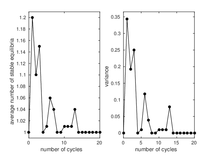
First, we fix $N=8$ and $K=100$ and investigate the number of stable equilibria for sparse random graphs. For each $c=0,1,\ldots,20$, we construct $100$ random graphs having exactly $c$ cycles. We achieve this by generating adjacency matrices of symmetric Erdős-Rényi random graphs until we have $100$ instances of connected graphs with the desired number of cycles. Depending on the graph, we find $1$, $2$, or $3$ stable equilibria. The averages of these results are shown in Figure 7 showing that the sparsest (i.e., acyclic) as well as sufficiently dense graphs have exactly one stable equilibrium confirming the analytic results for these two extremal topologies [23, 4, 21, 22, 24]. Since cycles are known to display multi-stability (see Figure 5), it is to be expected that there is more than one stable equilibrium for small cycle numbers. Quite surprisingly, multiple distinct extrema can be observed in the stable equilibrium distribution in Figure 7.

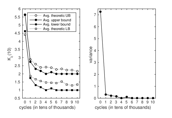
Next, we fix $N=10$ and investigate how $K_{c}(N)$ depends on the density of the graph. For each coupling probability $P=0.25,0.375,\ldots,0.875$, we generated $100$ random graphs. For each graph, we computed equilibria and determine stability at the following values of $K$: for $P=0.25$ we use $K=1,\ldots,20$; for $P=0.375$ we use $K=1,\ldots,15$; for $P=0.5$ we use $K=1,\ldots,10$; and for each $P=0.625,0.75,0.875$, we use $K=1,\ldots,5$. In all cases, we find a value of $K$ such that at least one stable equilibrium occurs at $K$ while no stable equilibria occur at $K-1$, thereby allowing us to estimate bounds on $K_{c}(10)$. Figure 8 shows these results sorted according to the number of cycles in the graph.

For undirected and connected graphs, a theoretic lower and a conjectured theoretic upper bound are [4, 23]

where $\textup{deg}_{i}=\sum_{j}a_{ij}$ is the degree of node $i$, $B$ is the oriented incidence matrix, and $L$ is the network Laplacian matrix. These bounds are shown in Figure 8 for comparison. We verified that our $600$ individual results as well as the averages shown are consistent with these theoretic bounds and validate their accuracy. Figure 8 indicates that the numerical upper bound is tighter than the theoretic bound on average, while the numerical lower bound tends to be weaker. Since the tightness of our computed bounds depends on the resolution of $K$ values tested, one could check more refined $K$ values to obtain tighter numerical bounds for particular graphs of interest.

In future work, we aim to extend our investigations to directed graphs, negative weights, cosine coupling, and statistical properties of random graph models, as well as verify conjectures for variations of the Kuramoto models as studied in Ref. [42].

References

- [1] Y. Kuramoto. In International symposium on mathematical problems in theoretical physics, pages 420–422. Springer, 1975.
- [2] J.A. Acebrón, L.L. Bonilla, C.J. Pérez Vicente, F. Ritort, and R. Spigler. Reviews of modern physics, 77(1):137, 2005.
- [3] S.H. Strogatz. Physica D: Nonlinear Phenomena, 143(1):1–20, 2000.
- [4] F. Dörfler and F. Bullo. Automatica, 50(6):1539–1564, June 2014.
- [5] L. Casetti, M. Pettini, and E.G.D. Cohen. Journal of Statistical Physics, 111:1091–1123(33), June 2003.
- [6] D. Mehta. Lattice vs. Continuum: Landau Gauge Fixing and ’t Hooft-Polyakov Monopoles. Ph.D. Thesis, The Uni. of Adelaide, Australasian Digital Theses Program, 2009.
- [7] D. Mehta and M. Kastner. Annals Phys., 326:1425–1440, 2011.
- [8] L. von Smekal, D. Mehta, A. Sternbeck, and A.G. Williams. PoS, LAT2007:382, 2007.
- [9] L. von Smekal, A. Jorkowski, D. Mehta, and A. Sternbeck. PoS, CONFINEMENT8:048, 2008.
- [10] R. Nerattini, M. Kastner, D. Mehta, and L. Casetti. Phys.Rev., E87(3):032140, 2013.
- [11] M. Kastner. Physical Review E, 83(3):031114, 2011.
- [12] C. Hughes, D. Mehta, and J.-I. Skullerud. Annals Phys., 331:188–215, 2013.
- [13] D. Mehta and M. Schröck. Phys. Rev. D 89 094512 (2014).
- [14] D. Mehta, A. Sternbeck, L. von Smekal, and A.G. Williams. PoS, QCD-TNT09:025, 2009.
- [15] J. Baillieul and C.I. Byrnes. IEEE Transactions on Circuits and Systems, 29(11):724–737, 1982.
- [16] A. Araposthatis, S. Sastry, and P. Varaiya. International Journal of Electrical Power & Energy Systems, 3(3):115–126, 1981.
- [17] S.H. Strogatz and R.E. Mirollo. Journal of Statistical Physics, 63(3-4):613–635, 1991.
- [18] M. Verwoerd and O. Mason. SIAM Journal on Applied Dynamical Systems, 8(1):417–453, 2009.
- [19] M. Verwoerd and O. Mason. SIAM Journal on Applied Dynamical Systems, 7(1):134–160, 2008.
- [20] F. Dörfler and F. Bullo. SIAM Journal on Applied Dynamical Systems, 10(3):1070–1099, 2011.
- [21] D. Aeyels and J.A. Rogge. Progress on Theoretical Physics, 112(6):921–942, 2004.
- [22] R.E. Mirollo and S.H. Strogatz. Physica D: Nonlinear Phenomena, 205(1-4):249–266, 2005.
- [23] F. Dörfler, M. Chertkov, and F. Bullo. Proceedings of the National Academy of Sciences, 110(6):2005–2010, 2013.
- [24] R. Taylor. Journal of Physics A: Mathematical and Theoretical, 45(5):055102, 2012.
- [25] J. Ochab and P.F. Góra. Synchronization of coupled oscillators in a local one-dimensional Kuramoto model. arXiv preprint arXiv:0909.0043, 2009.
- [26] P. F. C. Tilles, F. F. Ferreira and H. A. Cerdeira. Phys. Rev. E 83 066206 (2011).
- [27] A.P. Morgan and A.J. Sommese. Appl. Math. Comput., 29(2):123–160, 1989.
- [28] A.J. Sommese and C.W. Wampler. The Numerical Solution of Systems of Polynomials Arising in Engineering and Science. World Scientific Publishing, Hackensack, NJ, 2005.
- [29] D.J. Bates, J.D. Hauenstein, A.J. Sommese, and C.W. Wampler. Numerically solving polynomial systems with Bertini, volume 25. SIAM, 2013.
- [30] D. Mehta, H. Nguyen, and K. Turitsyn, “Numerical Polynomial Homotopy Continuation Method to Locate All The Power Flow Solutions,” arXiv:1408.2732 (2014).
- [31] S. Chandra, D. Mehta, and A. Chakrabortty, “Exploring the impact of wind penetration on power system equilibrium using a numerical continuation approach,” arXiv:1409.7844 (2014).
- [32] D. Mehta. Adv.High Energy Phys., 2011:263937, 2011.
- [33] M. Maniatis and D. Mehta. Eur.Phys.J.Plus, 127:91, 2012.
- [34] M. Kastner and D. Mehta. Phys.Rev.Lett., 107:160602, 2011.
- [35] D. Mehta, Y.-H. He, and J.D. Hauenstein. JHEP, 1207:018, 2012.
- [36] D. Mehta, J.D. Hauenstein, and M. Kastner. Phys. Rev. E, 85:061103, Jun 2012.
- [37] B. Greene, D. Kagan, A. Masoumi, D. Mehta, E.J. Weinberg, and Xiao Xiao. Phys.Rev., D88(2):026005, 2013.
- [38] D. Mehta, D.A. Stariolo, and M. Kastner. Phys.Rev., E87(5):052143, 2013.
- [39] D. Martinez-Pedrera, D. Mehta, M. Rummel, and A. Westphal. JHEP, 1306:110, 2013.
- [40] Y.-H. He, D. Mehta, M. Niemerg, M. Rummel, and A. Valeanu. JHEP, 1307:050, 2013.
- [41] D.J. Bates, J.D. Hauenstein, A.J. Sommese, and C.W. Wampler. Bertini: Software for numerical algebraic geometry. Available at http://bertini.nd.edu.
- [42] D. A. Wiley, S. H. Strogatz and M. Girvan. Chaos: An Interdisciplinary J. of Non. Sci., 16 015103 (2006).
- [43] S. H. Strogatz and R. E. Mirollo. Physica D: Non. Phen., 31, 143 (1988).
- [44] G. B. Ermentrout. J. Math. Bio.,23 55 (1985).