Sparse Variational Bayesian Approximations for Nonlinear Inverse Problems: applications in nonlinear elastography
Abstract
This paper presents an efficient Bayesian framework for solving nonlinear, high-dimensional model calibration problems. It is based on a Variational Bayesian formulation that aims at approximating the exact posterior by means of solving an optimization problem over an appropriately selected family of distributions. The goal is two-fold. Firstly, to find lower-dimensional representations of the unknown parameter vector that capture as much as possible of the associated posterior density, and secondly to enable the computation of the approximate posterior density with as few forward calls as possible. We discuss how these objectives can be achieved by using a fully Bayesian argumentation and employing the marginal likelihood or evidence as the ultimate model validation metric for any proposed dimensionality reduction. We demonstrate the performance of the proposed methodology for problems in nonlinear elastography where the identification of the mechanical properties of biological materials can inform non-invasive, medical diagnosis. An Importance Sampling scheme is finally employed in order to validate the results and assess the efficacy of the approximations provided.
Keywords:
Uncertainty Quantification, Variational Bayesian , Inverse Problem , Dimensionality reduction , Elastography , Dictionary LearningCopyright © 2015 I. M. Franck and P.S. Koutsourelakis. This manuscript version is made available under the CC-BY-NC-ND 4.0 license http://creativecommons.org/licenses/by-nc-nd/4.0/
1 Introduction
The extensive use of large-scale computational models poses several challenges in model calibration as the accuracy of the predictions provided depends strongly on assigning proper values to the various model parameters. In mechanics of materials, accurate mechanical property identification can guide damage detection and an informed assessment of the system’s reliability [1]. Identifying property-cross correlations can lead to the design of multi-functional materials [2]. Permeability estimation for soil transport processes can assist in detection of contaminants, oil exploration [3].
Deterministic optimization techniques which have been developed to address these problems [4], lead to point estimates for the unknowns without rigorously considering the statistical nature of the problem and without providing quantification of the uncertainty in the inverse solution. Statistical approaches based on the Bayesian paradigm [5] on the other hand, aim at computing a (posterior) probability distribution on the parameters of interest. Bayesian formulations offer several advantages as they provide a unified framework for dealing with the uncertainty introduced by the incomplete and noisy measurements. Significant successes have been noted in applications such as geological tomography [6] , medical tomography [7], petroleum engineering [8] , as well as a host of other physical, biological, or social systems [9, 10]. Representations of the parametric fields in existing deterministic and Bayesian approaches (artificially) impose a minimum length scale of variability usually determined by the discretization size of the governing PDEs [11]. As a result they give rise to a very large vector of unknowns. Inference in high-dimensional spaces using standard Markov Chain Monte Carlo (MCMC) schemes is generally impractical as it requires an exuberant number of calls to the forward simulator in order to achieve convergence. Advanced schemes such as those employing Sequential Monte Carlo samplers [12, 13], adaptive MCMC [14], accelerated MCMC methods [15] or spectral methods [16] can alleviate some of these difficulties particularly when the posterior is multi-modal but still pose significant challenges in terms of the computational cost [17].
This work is particularly concerned with the identification of the mechanical properties of biological materials, in the context non-invasive medical diagnosis. While in certain cases mechanical properties can also be measured directly by excising multiple tissue samples, non-invasive procedures offer obvious advantages in terms of ease, cost and reducing risk of complications to the patient. Rather than x-ray techniques which capture variations in density, the identification of stiffness or mechanical properties in general, can potentially lead to earlier and more accurate diagnosis [18, 19], provide valuable insights that differentiate between modalities of the same pathology [20] and monitor the progress of treatments. In this paper we do not propose new imaging techniques but rather aim at developing rigorous statistical models and efficient computational tools that can make use of the data/observables (i.e. noisy displacements of deformed tissue) from existing imaging modalities (such as magnetic resonance [21], ultrasonic) in order to produce certifiable estimates of mechanical properties. The primary imaging modality considered in this project is ultrasound elasticity imaging (elastography [22, 23]). It is based on ultrasound tracking of pre- and post-compression images to obtain a map of position changes and deformations of the specimen due to an external pressure/load. The pioneering work of Ophir and coworkers [24] followed by several clinical studies [25, 26, 27] have demonstrated that the resulting strain images typically improve the diagnostic accuracy over ultrasound alone.
Beyond a mere strain imaging there are two approaches for inferring the constitutive material parameters. In the direct approach, the equations of equilibrium are interpreted as equations for the material parameters of interest, where the inferred strains and their derivatives appear as coefficients [28]. While such an approach provides a computationally efficient strategy, it does not use the raw data (i.e. noisy displacements) but transformed versions i.e. strain fields (or even-worse, strain derivatives) which arise by applying sometimes ad hoc filtering and smoothing operators. As a result the informational content of the data is compromised and the quantification of the effect of observation noise is cumbersome. Furthermore, the smoothing employed can smear regions with sharply varying properties and hinder proper identification.
The alternative to direct methods, i.e. indirect or iterative procedures admit an inverse problem formulation where the discrepancy between observed and model-predicted displacements is minimized with respect to the material fields of interest [29, 30, 31, 32]. While these approaches utilize directly the raw data, they generally imply an increased computational cost as the forward problem and potentially derivatives have to be solved/computed several times. This effort is amplified when stochastic/statistical formulations are employed as those arising in the Bayesian paradigm. Technological advances have led to the development of hand-carried ultrasound systems in the size of a smartphone [33]. Naturally their accuracy and resolution does not compare with the more expensive traditional ultrasound machines or even more so MRI systems. If however computational tools are available that can distill the informational content from noisy and incomplete data then this would constitute a major advance. Furthermore, significant progress is needed in improving the computational efficiency of these tools if they are to be made applicable on a patient-specific basis.
In this work we advocate a Variational Bayesian (VB) perspective [34, 35]. Such methods have risen into prominence for probabilistic inference tasks in the machine learning community [36, 37, 38] but have recently been employed also in the context of inverse problems [39, 40]. They provide approximate inference results by solving an optimization problem over a family of appropriately selected probability densities with the objective of minimizing the Kullback-Leibler divergence [41] with the exact posterior. The success of such an approach hinges upon the selection of appropriate densities that have the capacity of providing good approximations while enabling efficient (and preferably) closed-form optimization with regards to their parameters. We note that an alternative optimization strategy originating from a different perspective and founded on map-based representations of the posterior has been proposed in [42].
A pivotal role in Variational Bayesian strategies or any other inference method, is dimensionality reduction i.e. the identification of lower-dimensional features that provide the strongest signature to the unknowns and the corresponding posterior. Discovering a sparse set of features has attracted great interest in many applications as in the representation of natural images [43] and a host of algorithms have been developed not only for finding such representations but also an appropriate dictionary for achieving this goal [44]. While all these tools are pertinent to the present problem they differ in a fundamental way. They are based on several data/observations/instantiations of the vector that we seek to represent. In our problem however we do not have such direct observations i.e. the data available pertains to the output of a model which is nonlinearly and implicitly dependent on the vector of unknowns. Furthermore we are primarily interested in approximating the posterior of this vector rather than the dimensionality reduction itself. We demonstrate how this can be done by using a fully Bayesian argumentation and employing the marginal likelihood or evidence as the ultimate model validation metric for any proposed dimensionality reduction.
The paper is organized as follows: The next section (Section 2) presents the essential ingredients of the forward model (Section 2.1) which are common with a wide range of nonlinear, high-dimensional problems encountered in several simulation contexts. We also discuss the VB framework advocated, the dimensionality reduction scheme proposed, the prior densities for all model parameters, an iterative, coordinate-ascent algorithm that enables the identification of all the unknowns (Section 2.2) as well as an information-theoretic criterion for determining the number of dimensions needed (Section 2.3). We finally describe a Monte Carlo scheme based on Importance Sampling that can provide statistics of the exact posterior as well as a quantitative assessment of the VB approximation (Section 2.4). Section 3 demonstrates the performance and features of the proposed methodology in two problems from solid mechanics that are of relevance to the elastography settings. Various signal-to-noise ratios are considered and the performance of the method, in terms of forward calls and accuracy, is assessed.
2 Methodology
The motivating application is related to continuum mechanics in the nonlinear elasticity regime. We describe below the governing equations in terms of conservation laws and the constitutive equations. The proposed model calibration process can be readily adapted to other forward models. As it will be shown, the only information utilized by the Bayesian inference engine proposed is a) the response quantities at the locations where measurements are available, and b) their derivatives with respect to the unknown model parameters.
2.1 Forward model - Governing equations
The following expressions are formulated in the general case which includes nonlinear material behavior and large deformations. Our physical domain is described by in in the reference configuration. Let denote the coordinates of the continuum particles in the undeformed configuration and in the deformed. Their relation (in the static case) is provided by the deformation map such that: . The displacement field is defined as . The gradient of the deformation map is denoted by and is then the Lagrangian (finite) strain tensor used as the primary kinematic state variable in our constitutive law [45, 46, 47]. The governing equations consist of the conservation of linear momentum:
| (1) |
and the Dirichlet and Neumann boundary conditions as
| (2) |
| (3) |
b is body force vector (per unit mass), is the initial density, S is the second Piola-Kirchhoff stress tensor and is the outward normal at . and are subsets of the boundary, , on which displacement and traction boundary data, and , respectively, are specified. For a hyperelastic material, it is assumed that the strain energy density function exists and depends on the invariants of the Lagrangian strain tensor E and the constitutive material parameters . We note that the latter in general exhibit spatial variability which we intend to estimate using the methods discussed. The conjugate stress variables described by the second Piola-Kirchhoff stress tensor can be found as:
| (4) |
The aforementioned governing equations should be complemented with any other information about the problem or the material, such as incompressibility. In fact incompressibility is frequently encountered in bio-materials and corresponds to the condition at all points in the problem problem domain.
The governing equations presented thus far cannot be solved analytically for the vast majority of problems and one must resort to numerical techniques that discretize these equations and the associated fields. The most prominent such approach is the Finite Element Method (FEM) which is employed in this study as well. In the first step, the weak form of the PDEs needs to be derived. To that end, we define the usual function spaces and for the set of admissible solutions and weighting functions respectively, as follows [48]:
| (5) |
where denotes the Sobolev space of square integrable functions with square integrable derivatives in [49]. By multiplying Equation (1) with a weighting function , integrating by parts and exploiting the essential and non-essential boundary conditions above, we obtain:
| (6) |
In the incompressible case, pressure must be taken into account and for that purpose the pressure trial solutions and weighting functions should also be introduced [50].
Subsequently the problem domain is discretized into finite elements and shape functions are used for interpolating the unknown fields. As this is a very mature subject, from a theoretical and computational point of view, we do not provide further details here but refer the interested reader to one of many books available [51, 52] or more specifically in the context of inverse problems for (in)compressible elasticity in [48, 50]. Most often all unknowns are expressed in terms of the discretized displacement field denoted here by a vector . An approximate solution can be found by solving an dimensional system of nonlinear algebraic equations which in residual form can be written as:
| (7) |
We denote here by the residuals and by , the discretized vector of constitutive material parameters .
The discretizations can be done in many different ways. For example if the same mesh and shape functions as for the discretization of the displacements are adopted, then each entry of the vector corresponds to the value of the material parameter of interest at each nodal point. Frequently it is assumed that the value of the constitutive parameters are constant within each finite element in which case coincides with the number of elements in the FE mesh. While the representation of is discussed in detail in the sequence, we point out that the discretization of does not need to be associated with the discretization used for the governing equations. Usually in practice the two are related, but if one aims at inferring as many details about the variability of that the discretized equations can provide, a finer discretization might be employed for . We note however that if the material properties exhibit significant variability within each finite element i.e. if , special care has to be taken in formulating the finite element solution and multiscale schemes might need to be employed [53].
We note here:
- 1.
Frequently the size of the system of the equations that need to be solved is large. This is necessitated by accuracy requirements in capturing the underlying physics and mathematics. It can impose a significant computational burden as in general repeated solutions of this system, under different values of , are needed. If for example a Newton-Raphson method is employed then repeated solutions of the linearized Equation (7) will need to be performed:
(8) where is the iteration number and is the Jacobian matrix. Hence for large as in applications of interest, the number of such forward solutions is usually what dictates the overall computational cost and this is what we report in subsequent numerical experiments. Depending on the particular solution method employed, converged solutions at a certain stage of the inversion procedure can be used as initial guesses for subsequent solutions under different reducing as a result the overall cost. In this work we do not make use of such techniques.
- 2.
The data available generally concerns a subset or more generally a lower-dimensional function of . In this work, the experimental measurements/ observations are (noisy) displacements at specific locations in the physical domain. We denote these displacements by and they can be formally expressed as where is a Boolean matrix which picks out the entries of interest from . Naturally, since depends on , is also a function of i.e. . We emphasize that this function is generally highly nonlinear and most often than not, many-to-one [54]. The unavailability of the inverse as well as the high nonlinearity constitute two of the basic difficulties of the associated inverse problem.
- 3.
In addition to the solution vector , the proposed inference scheme will make use of the derivatives . The computation of derivatives of the response with respect to model parameters is a well-studied subject in the context of PDE-constrained optimization [55, 56, 57] and we make use of it in this work. For any scalar function , one can employ the adjoint form of Equation (7) according to which:
(9) where is defined such as:
(10) We note that is the Jacobian of the residuals in Equation (7) evaluated at the solution . We point out that if a direct solver for the solution of the linear system in is employed, then the additional cost of evaluating is minimal as the Jacobian would not need to be re-factorized for solving Equation (10) 11 1 The cost of evaluating is negligible compared to other terms as it scales linearly with the number of elements/nodes.. In the context of the problems considered in this paper (see Section 3), repeated use of Equation (10) is made where is a different component of the observables and as such the overall cost increases proportionally with the number of observables (displacements in our problems) that are available. In problems where is so large that it precludes the use of direct solvers, then the cost of its solution of the adjoint equations can be augmented but nevertheless comparable to the cost of a forward solution. In cases where both as well as the dimension of are high, then advanced iterative solvers, suitable for multiple right-hand sides must be employed [58, 59]. These imply an added computational burden which nevertheless scales sublinearly with the dimension of .
2.2 Bayesian Model
The following discussion is formulated in general terms and can be applied for the calibration of any model with parameters represented by the vector when output is available. We also presuppose the availability of the derivatives . For problems of practical interest, it is assumed that the dimension of the unknowns is very large which poses a significant hindrance in the solution of the associated inverse problem as well as in finding proper regularization (in deterministic settings [60]) or in specifying appropriate priors (in probabilistic settings [61, 62]). The primary focus of the Bayesian model developed is two-fold:
- 1.
find lower-dimensional representations of the unknown parameter vector that capture as much as possible of the associated posterior density
- 2.
enable the computation of the posterior density with as few forward calls (i.e. evaluations of ) as possible.
We denote the vector of observations/measurements. In the context of elastography the observations are displacements (in the static case) and/or velocities (in the dynamics). The extraction of this data from images (ultrasound or MRI) is a challenging topic that requires sophisticated image registration techniques [63, 64]. Naturally, these compromise the informational content of the raw data (i.e. the images). In this study we ignore the error introduced by the image registration process, as the emphasis is on the inversion of the continuum mechanics, PDE-based, model, and assume that the displacement data are contaminated with noise. We postulate the presence of i.i.d. Gaussian noise denoted here by the random vector such that:
| (11) |
We assume that each entry of has zero mean and an unknown variance which will also be inferred from the data. We note that other models can also be employed as for example impulsive noise to account for outliers due to instrument calibration or experimental conditions [65]. Generally the difference between observed and model-predicted outputs can be attributed not only to observation errors (noise) but also to model discrepancies [66, 67, 68]. In this work such model errors are lumped with observation errors in the -term.
The likelihood function of the observed data i.e. its conditional probability density given the model parameters (and implicitly the model itself as described by the aforementioned governing Equations (7)) and is:
| (12) |
In the Bayesian framework advocated one would also need to specify priors on the unknown parameters. We defer a detailed discussion of the priors associated with for the next section where the dimensionality reduction aspects are discussed. With regards to the noise precision we employ a (conditionally) conjugate Gamma prior i.e.
| (13) |
The values of the parameters are taken in the following examples. This corresponds to a limiting case where the density degenerates to an improper, non-informative Jeffreys prior i.e. that is scale invariant [69]. Naturally more informative choices can be made if such information is available a priori.
2.2.1 Dimensionality Reduction for
As mentioned earlier one of the primary goals of the present work to is identify, with the least number of forward calls, a lower-dimensional subspace in on which the posterior probability density can be sufficiently-well approximated. Dimensionality reduction could be enforced directly by appropriate prior specification. For example in [70] the Fourier transform coefficients of corresponding to small-wavelength fluctuations were turned-off by assigning zero prior probability to non-zero values. While such an approach achieves the goal of dimensionality reduction it does not take into account the forward model in doing so. The nonlinear map as well as the available data provide varying amounts of information for identifying different features of . One would expect the likelihood (which measures the degree of fit of model predictions with the data) to exhibit different levels of sensitivity along different directions in the -space. Consider for example Laplace’s method which is based on a semi-analytic Gaussian approximation around the Maximum-A-Posteriori estimate [71, 35]. The negative of the Hessian of the log-posterior (assuming this is positive-definite) serves as the covariance matrix. As it was shown in [72] in many inverse problems this covariance matrix exhibits a significant discrepancy in its eigenvalues which was exploited in constructing low-rank approximations. At one extreme, there would be principal directions (with small variance) along which the slightest change from from would cause a huge decrease in the posterior and on the other, there would principal directions (with large variance) along which the posterior would remain almost constant. Such principal directions will naturally encapsulate the effect of the log-prior. In the proposed scheme however, only the data log-likelihood affects the directions with the maximal posterior variance [73]. More importantly perhaps we propose a unified framework where the identification of the subspace with the largest posterior variance is performed simultaneously with the inference of the posterior under the same Variational Bayesian objective. This yields not only a highly efficient algorithm (in terms of the number of forward solves) but also a highly extendable framework as discussed in the conclusions.
The inference and dimensionality reduction problems are approached by employing fully Bayesian argumentation and invoking the quality of the approximation to the posterior as our guiding objective. To that end we postulate the following representation for the high-dimensional vector of unknowns :
| (14) |
The motivation behind such a decomposition is quite intuitive as it resembles a Principal Component Analysis (PCA) model [74]. The vector represents the mean value of the representation of whereas the reduced (and latent) coordinates of along the linear subspace spanned by the columns of the matrix . The linear decomposition of a high-dimensional vector such as has received a lot of attention in several different fields. Most commonly represents a high-dimensional signal (e.g. an image, an audio/video recording) and consists of an over- or under-complete basis set [43, 75] which attempts to encode the signal as sparsely as possible. Significant advances in Compressed Sensing [76] or Sparse Bayesian Learning [77] have been achieved in recent years along these lines. A host of deterministic [78] or probabilistic [79] algorithms have been developed for identifying the reduced-coordinates (or their posterior) as well as techniques for learning the most appropriate set of basis (dictionary learning) i.e. the one that can lead to the sparsest possible representation. While all these tools are pertinent to the present problem they differ in a fundamental way. They are based on several data/ observations/instantiations of whereas in our problem we do not have such direct observations i.e. the data available pertains to which is nonlinearly and implicitly dependent on . Furthermore we are primarily interested in approximating the posterior on rather than the dimensionality reduction itself.
We focus now on the representation of Equation (14) and proceed to discuss the identification of , and . In a fully Bayesian setting these parameters would be equipped with priors, say respectively22 2 We use the same symbol for various densities without super/subscripts for economy of notation. The parameters each density pertains to, can be identified from its arguments., and their joint posterior would be sought:
| (15) |
where represents the Gamma prior for discussed in Equation (13). Such an inference problem would in general be formidable particularly with regards to and whose dimension is dominated by . To address this difficulty we propose computing point estimates for and while inferring the whole posterior of . In doing so for and the natural objective function would be the marginal posterior :
| (16) |
In such a case the point estimates for would be the Maximum-a-Posteriori-Estimates (MAP). We note that (up to an additive constant):
| (17) |
We note that such an integration is analytically impossible primarily due to the nonlinear and implicit nature of and secondarily due to the coupling of and . To that end we employ a Variational Bayesian approximation [35] to the integral in Equation (17). We provide further details in the next section. We note that similar approximations have been employed in previous works [40, 65, 39] in order to expedite Bayesian inference. The novel element of this work pertains to the dimensionality reduction that can be achieved.
2.2.2 Variational Bayesian approximation
Consider an arbitrary joint density on the latent variables . Then by employing Jensen’s inequality one can construct a lower bound to the log-marginal-posterior in Equation (17) as follows:
| (18) |
We note here that the variational lower-bound has an intimate connection with the Kullback-Leibler divergence between and the (conditional) posterior on :
| (19) |
In particular, if we denote by is the expectation with regards to :
| (20) |
By definition the KL-divergence is non-negative and it becomes when . Hence , for a given , constructing a good approximation to the conditional posterior (in the KL-divergence sense) is equivalent to maximizing the lower bound with regards to .
The aforementioned discussion suggests an iterative optimization scheme that resembles the Variational Bayes - Expectation-Maximization (VB-EM) methods that have appeared in Machine Learning literature [34]. At each iteration , one alternates between (Figure 1):
- 1.
VB-Expectation: Given , find:
(21) - 2.
VB-Maximization: Given , find:
(22)
In plain terms, the strategy advocated in order to carry out the inference task can be described as a generalized coordinate ascent with regards to (Figure 2).
To alleviate the difficulties with the log-likelihood integral above we employ the following approximations:
- 1.
We linearize the map at . Hence:
(25) where is the gradient of the map at .
By keeping the first order terms from Equation (25) , the term in the exponent of the likelihood becomes:
(26) We note here that a quadratic expression with respect to could also be obtained by considering the order Taylor series of around directly. In particular if we denote by and and keeping only up to second order terms yields:
(27) The computation of order derivatives can also be addressed within the adjoint framework. We refer the interested reader to [56, 80] as we do not pursue this possibility further in this work. The ensuing expressions are based on Equation (26) but can be readily adjusted to include the terms in Equation (27) instead 33 3 The only additional requirement is that is semi-positive definite or that a semi-positive approximation is used..
We note that by making use of the linearization of the map and the Variational Bayesian approximation, one can obtain a tractable approximations of the posterior of the latent parameters and . This will enable us to ultimately identify all model parameters and through this process the optimal subspace for approximating the posterior on . This will be explained in detail when the final algorithm is presented in section 2.2.4.
- 2.
The aforementioned equations for the VB-Expectation step imply that probabilistic inference can be expressed in terms of a parametric optimization problem. One can adopt a functional form for depending on an appropriate set of parameters and identify their optimal value by minimizing the KL-divergence with the posterior or equivalently maximizing . We adopt a mean-field approximation where one looks for factorized densities of the form:
(28) Variational mean-field approximations have their origin in statistical physics [81]. We make these expressions more specific in the next sections where we discuss the prior for as well.
2.2.3 Prior Specification for and
We discuss first the prior specification on . Its columns span the subspace over which an approximation of is sought. We note that depends on the product which would remain invariant by appropriate rescaling of each pair of and for any . Hence, to resolve identifiability issues we require that is orthogonal i.e. where is the dimensional identity matrix. This is equivalent to employing a uniform prior on on the Stiefel manifold [82].
The latent, reduced coordinates capture the variation of around its mean along the directions of as implied by Equation (14). It is therefore reasonable to assume that, a priori, these should have zero mean and should be uncorrelated [74]. For that purpose we adopt a multivariate Gaussian prior (denoted by in the Equations of the previous section) with a diagonal covariance denoted by . We select prior variances such that . This induces a natural (stochastic) ordering to the reduced coordinates since is invariant to permutations of the entries of the and the columns of (Equation (14)). As a result of this ordering, is associated with the direction along which the largest variance in is attained, with the direction with the second largest variance and so on. We discuss the particular values given to prior hyperparameters in the sequel (Section 3) and in Section 2.3 the possibility of an adaptive decomposition is also presented. This enables the sequential addition of reduced coordinates until a sufficiently good approximation to the posterior is attained.
The final aspect of the prior model pertains to . We use a hierarchical prior that induces the requisite smoothness given that represents the spatial variability of the material parameters. In particular the prior model employed penalizes the jumps in the values of and which correspond to neighboring sites/locations . The definition of a neighborhood can be adjusted depending on the problem, but in this work we assume that sites/locations belong to the neighborhood if the they correspond to adjacent pixels/voxels. Suppose is the total number of jumps or neighboring pairs. Then for if and denote the corresponding neighboring pair:
| (29) |
The strength of the penalty is proportional to the hyperparameter , i.e. smaller values of induce a weaker penalty and vice versa. Let the denote the Boolean matrix that can be used to produce the vector of all jumps (as the one above) between all neighboring sites from the vector as , and the diagonal matrix containing all the hyperparameters associated with each of these jumps. We can represent the combined prior on as:
| (30) |
A conjugate prior of the hyperparameters is a product of Gamma distributions:
| (31) |
As in [83] the independence is motivated by the absence of correlation (a priori) with regards to the locations of the jumps. In this work we use which corresponds to a limiting case of a Jeffreys prior that is scale invariant. We note that in contrast to previous works where such priors have been employed for the vector of unknowns and MAP estimates have been obtained [5], we employ this here for which is only part of the overall decomposition in Equation (14). We discuss in the following section the update equations for and the associated hyper-parameters as well as for the remaining model variables.
2.2.4 Update equations for
We postulate first that the reduced coordinates should a posteriori have zero mean as they capture variability around . For that purpose we confine our search for to distributions with zero mean. Given the aforementioned prior and the linearization discussed in the previous section, we can readily deduce from Equation (23) that the optimal approximate posteriors and under the mean-field Variational Bayesian scheme adopted will be:
| (32) |
The associated parameters are given by the following iterative Equations:
| (33) |
| (34) |
where .
As a result of the aforementioned Equations and Equation (14), one can establish that the posterior of is approximated by a Gaussian with mean and covariance given by:
| (35) |
We note that if we diagonalize i.e. where is diagonal and is orthogonal with columns equal to the eigenvectors of , then:
| (36) |
where is also orthogonal (i.e. ) and contains the principal directions of the posterior covariance of . Hence it suffices to consider approximate posteriors with covariance that is diagonal i.e. . In this case the update equations for in Equation (34) reduce to:
| (37) |
We note that despite the prior assumption on uncorrelated , the posterior on exhibits correlation and captures the principal directions along which the variance is largest. Furthermore, implicit to the aforementioned derivations is the assumption of a unimodal posterior on and subsequently on . This assumption can be relaxed by employing a mixture of Gaussians (e.g. [84]) that will enable the approximation of highly non-Gaussian and potentially multi-modal posteriors. Such approximations could also be combined with the employment of different basis sets for each of the mixture component which would provide a wide range of possibilities. We defer further discussions along these lines to future work. In the examined elastography applications, the unimodal assumption seems to be a reasonable one due to the generally large of amounts of data/observations obtained from various imaging modalities.
Given the aforementioned results one can obtain an expression for the variational lower bound in Equation (23). For economy of notation we use to denote expectations with respect to and/or as implied by the arguments:
| (38) |
where is the normalization constant of a distribution with parameters . The aforementioned equation can be further simplified by making use of the following expectations: , :
| (39) |
In order to update in the VB-Maximization step, it suffices to consider only the terms of that depend on it which we denote by i.e.:
| (40) |
As discussed earlier the prior enforces the orthogonality constraint on . To address this constrained optimization problem, we employ the iterative algorithm proposed in [85] which has proven highly efficient in terms of the number of iterations and the cost per iterations in several settings. It employs the Cayley transform to preserve the constraint during the optimization and makes use only of first order derivatives:
| (41) |
In brief, if is the skew-symmetric matrix:
| (42) |
the update equations are based on a Crank-Nicholson-like scheme:
| (43) |
where is the step size. One notes that the aforementioned update preserves the orthogonality of ([85]). In order to derive a good step size we use the Barzilai-Borwein scheme [86] which results in a non-monotone line search algorithm:
| (44) |
where represents the difference between the current parameter values as compared to the previous step. As discussed in detail in [85] the inversion of the matrix in Equation (43) can be efficiently performed by inverting a matrix of dimension which is much smaller than . We note that the updates of require no forward calls for the computation of or its derivatives . The updates/iterations are terminated when no further improvement to the objective is possible.
The final component involves the optimization of . As with we consider only the terms of (Equation (39)) that depend on which we denote by i.e.:
| (45) |
Due to the analytical unavailability of and its derivatives we employ here an Expectation-Maximization scheme [87, 88] which we describe in A for completeness. The output of this algorithm is also the posterior on the hyperparameters in Equation (29) which capture the locations of jumps in as well as the probabilities associated with them. The cost of the numerical operations is minimal and scales linearly with the number of neighboring pairs . In the following we simply make use of Equations (65) without further explanation.
Formally the determination of the optimal would require the derivatives in Equation (45). We note that depends on . Hence finding would require the computation of second-order derivatives of which poses significant computational difficulties in the high-dimensional setting considered. To avoid this and only for the purpose of the updates, we linearize Equation (45) around the current guess by ignoring the dependence of on or equivalently by assuming that remains constant in the vicinity of the current guess. In particular, let denote the value of at iteration , then in order to find the increment , we define the new objective as follows:
| (46) |
We note that there is no approximation with regards to the prior term. By keeping only the terms depending on in the Equation above we obtain:
| (47) |
This is a concave and quadratic with respect to the unknown . The maximum can be found by setting which yields:
| (48) |
We note that the exact objective is evaluated at and is accepted only if the value of the objective is larger than that at . Iterations at terminated when no further improvement is possible. Finally it was found that activating the regularization term () after five updates/iterations during which the optimization is performed solely on the basis of , enabled better exploration of the feasible solutions.
We summarize below the basic steps of the iterative Variational Bayesian scheme proposed in Algorithm 1.
With regards to the overall computational cost we note that the updates of are the most demanding as they require calls to the forward model to evaluate and the derivatives . The updates were terminated when no further increase in (Equation (39)) can be attained.
2.3 Adaptive learning - Cardinality of reduced coordinates
The presentation thus far was based on a fixed number of reduced coordinates . A natural question that arises is how many should one consider. In order to address this issue we propose an adaptive learning scheme. According to this the analysis is first performed with a few (even one) reduced coordinates and upon convergence additional reduced coordinates are introduced, either in small batches or even one-by-one. Critical to the implementation of such a scheme is a metric for the progress achieved by the addition of reduced coordinates and basis vectors which can also be used as a termination criterion.
In this work we advocate the use of an information-theoretic criterion which measures the information gain between the prior beliefs on and the corresponding posterior. To measure such gains we employ again the KL-divergence between the aforementioned distributions [89]. In particular if (section 2.2.3) and (Equation (37)) denote the dimensional prior and posterior respectively, we define the quantity as follows:
| (49) |
which measures the (relative) information gain from to reduced coordinates. The KL divergence between and with and where are diagonal as explained previously follows with:
| (50) |
and equation (49) becomes:
| (51) |
In the simulations performed in section 3, we demonstrate the evolution of this metric as reduced-coordinates/basis vectors are added one-by-one. The addition of reduced coordinates was terminated when was below for at least five consecutive . In Figure 3 an overview flowchart of the proposed algorithm is shown which incorporates the VB algorithm including dictionary learning from Algorithm 1 and the information gain assessment to identify the necessary number of basis vectors from this subsection.
-update: W-update: q-update:
2.4 Validation - Combining VB approximations with Importance Sampling
Thus far we have employed the variational lower bound in order to identify the optimal dimensionality reduction and to infer the latent variables that approximate the posterior. The goal of this section is twofold. Firstly to show how the biased VB approximation can be used in order to obtain efficiently, (asymptotically) unbiased estimates with regards to the true posterior and secondly to assess (quantitatively) the accuracy of the VB approximation. To that end we employ Importance Sampling (IS) with the variational posterior as the importance sampling distribution. We can thusly obtain consistent estimators of several exact posterior quantities as well as to measure the efficiency of IS.
Consider the exact posterior . We note that when is unknown as in the cases considered herein, the (marginal) likelihood can be determined by integrating with respect to . With the conjugate Gamma prior adopted (Equation (13)) this can be done analytically and would yield:
| (52) |
In cases where non-conjugate priors for are employed, the IS procedure detailed here has to be performed in the joint space (.
The evidence:
| (53) |
as well as the expectation of any function with regards to the exact posterior :
| (54) |
can be estimated using IS with respect to the IS density as follows:
| (55) |
where the samples are independent draws from and the IS weights are given by:
| (56) |
An indicator of the efficacy of the IS density is the (normalized) Effective Sample Size (ESS) which provides a measure of the degeneracy in the population of particles/samples as quantified by their variance [90]:
| (57) |
The latter attains values between the following extremes. If coincides with the exact posterior then all the importance weights would be equal and . On the other hand if provides a poor approximation then the expression for the is dominated by the largest weight and would yield (as ). The normalized ESS can be compared with that of MCMC [91]:
| (58) |
where is the autocovariance between MCMC states that are steps apart.
In summary, the VB framework advocated introduces approximations due to the linearization of the response (Equation (25)) and the mean field approximation (Equation (28)). To assess the bias of these approximations in the posterior inferred, we employ IS as explained above. This can lead to accuracy metrics (e.g. ESS) but more importantly can produce (asymptotically) unbiased statistics with regards to the exact posterior i.e. the one obtained without the approximations mentioned earlier. These metrics can be readily compared with those of alternative strategies (e.g. MCMC as in Equation (58)). Unequivocally, another important source of error is due to model discrepancies. That is, if the difference between observables and model predictions in Equation (11) is not valid due missing physics, discretization errors etc, then the inference results will deviate from reality, irrespectively of the numerical tools one employs [66, 67, 68]. We emphasize that the methodology proposed, as most strategies for the solution of inverse problems, is based on the assumption that model errors are zero or in any case much smaller than the observation errors.
3 Numerical Illustrations
The examples presented are concerned with the probabilistic identification of material parameters from displacement data. We demonstrate the efficacy of the proposed methodology in two, two-dimensional cases where synthetic displacement data are utilized. The data are contaminated with noise as discussed in the sequence. The first example is based on a linear elastic material model. The second example is based on the Mooney-Rivlin material model which is used to model nonlinear and incompressible response.
In the computations we use . We employ the adaptive learning scheme discussed in section 2.3 whereby reduced-coordinates/basis vectors are added one-by-one. The first reduced coordinate is assigned the broadest prior i.e. is the smallest of all other and captures the largest expected (a priori) variance. For subsequent bases we assign values to the precision parameters as follows:
| (59) |
We note that corresponds to the posterior precision for the previous reduced coordinate as found in Equation (37) according to which . This essentially implies that, a priori, the next reduced coordinate will have the precision of the previous one as long as it is larger than the threshold . Since by construction , we have that .
The most important quantities and dimensions of the ensuing two examples are summarized in table 1.
| Example 1 | Example 2 | |
|---|---|---|
| Dimension of observables: | ||
| Dimension of latent variables: | ||
| Dimension of reduced latent variables: | ||
| Nr. of forward calls |
3.1 Example 1: Linear elastic material
The primary objective of the first example is to assess the performance of the proposed framework in terms of accuracy and dimensionality reduction in a simple problem with the absence of model errors. For that purpose we consider a linear, isotropic elastic material model where the stress-strain relation is given by:
| (60) |
where is the elasticity tensor [46]. It is given by:
| (61) |
where is the elastic modulus. The second material parameter is the Poisson’s ratio which in this example is assumed known (). The vector of unknown parameters consists of the values of the elastic moduli at each finite element. We assume that the elastic modulus can take two values and such that . The ratio is representative of ductal carcinoma in situ in glandular tissue in the breast under a strain of [92]. The spatial distribution of the material is shown in Figure 5. The problem is with units. We employ a FE mesh. Displacement boundary conditions are employed which resemble those encountered when static pressure is applied on a tissue with the ultrasound transducer invoking a strain as depicted in Figure 4. In particular the boundary displacements at the bottom () are set to zero and at the top () the vertical displacements are set to and the horizontal displacements equal to zero. The vertical edges () are traction-free.
The parameter values are at the top row of elements are assumed known and equal to the exact values () otherwise any solutions for which would yield the same likelihood [48]. The displacements generated using the reference configuration were subsequently contaminated with Gaussian noise such that the resulting Signal-to-Noise Ratio (SNR) was . We adopt a very vague prior i.e. .


In the top row of Figure 6 various aspects of the posterior of the elastic moduli using 90 basis vectors, (equal to the total number of unknowns), are depicted and are compared with the corresponding results (second row). One can see that the inferred posterior means are practically identical and coincide with the ground truth. The same can be said for the posterior variances which can be capture to a large extent by employing only reduced coordinates.


A more detailed comparison of the inferred posterior for various is depicted in Figure 7.

Figure 8 depicts the relative information gain (as defined in Section 2.3) and the number of forward calls (which determines the computational cost) as a function of the number of reduced coordinates/basis vectors. One can notice that the information gain drops to relatively small values only after a small number of reduced coordinates (after the , it drops below ). For the posterior approximation obtained with (which as shown earlier is practically indistinguishable from the full-order result with ) only forward calls are needed. These forward calls, are performed at and for additional reduced coordinate no further forward calls are needed. A more detailed account of the optimization with regards to the model parameters and can be seen in Figure 9 where the evolution of the corresponding variational objectives and (Section 2.2.4) is plotted. We note again that the updates are the only ones that require forward calls. The optimization results with regards to are shown for . These are performed using the Barzilai-Borwein step size selection discussed previously which results in a non-monotone but robust optimization.


The most important basis vectors can be seen in Figure 10, in decreasing order, based on the corresponding variance .


Finally, the posterior of is depicted in Figure 11. One can observe that the magnitude is captured correctly, compared to the exact value, i.e. the corresponding variance of the Gaussian noise with which the data was contaminated.

The aforementioned results were validated by employing Importance Sampling as discussed in Section 2.4. The Effective Sample Size (ESS , Equation (57)) was (for ) which suggests a good approximation to the actual posterior is provided by then VB result [93]. More importantly, as it is shown in Figures 12 and 13, the first and second-order statistics of the exact posterior (estimated with Importance Sampling) and the VB approximation.


3.2 Incompressible Mooney-Rivlin material
Nonlinear, hyperelastic models have been successfully used in the past to describe the behavior of several biomaterials [94, 95, 18]. In this example we employ the Mooney-Rivlin model [96, 97] that is characterized by the following strain energy density function (Equation (4)):
| (62) |
where is the bulk modulus, and where are the first and second invariants of the of the left Cauchy-Green deformation tensor . The last term in Equation (62) is related to volumetric deformations whereas the first two terms to distortional. We consider here an incompressible material, i.e. , in which case the bulk modulus plays the role of a penalty parameter that enforces this constraint. We employ the three-field Hu-Washizu principle in order to enforce incompressibility and suppress volumetric locking [98, 51]. The three-field formulation requires a separate integration rule for the dilatational stiffness contribution. The bulk modulus is chosen as a function of with . We use [98, 99]. The higher is, the stronger is the incompressibility constraint.
In this example we assume which reduces the model to an uncoupled version of the incompressible neo-Hookean model [46]. The remaining parameter is assumed to vary in the problem domain which can be seen in Figure 14. In this example we have two inclusions, an elliptic and a circular inclusion, with different material properties. In the larger, elliptic inclusion (red), in the smaller, circular inclusion (orange) and in the remaining material (blue). The problem domain is with . It is discretized with finite elements of equal size and the governing equations are solved under plane strain conditions. The following boundary conditions are employed: both displacements are set to zero at the bottom () and a vertical distributed load in the vertical direction (pointing downwards) is applied along the top i.e. . The vertical edges () are traction-free.
The forward model for the Bayesian identification employed a regular mesh and only the corresponding (noisy) displacements at the nodes were used as data (). We note that due to the different meshes employed the data will also contain model (discretization) errors. The SNRs reported in the sequence include also these errors. We further assumed that was constant within each of the elements which resulted in unknowns. Using the displacements obtained from the fine mesh we consider three settings:
- 1.
Case A (high SNR/low noise): without additional noise resulting in a SNR .
- 2.
Case B (medium SNR/medium noise): the data are contaminated with relatively smaller Gaussian noise resulting in a total SNR .
- 3.
Case C (small SNR/high noise): the data are contaminated with relatively larger Gaussian noise resulting in a total SNR .
The results presented in the sequence were obtained for and the material parameters are plotted in the log-scale.

Figure 15 depicts the posterior mean for the aforementioned three cases. Figure 16 depicts the spatial distribution of the posterior standard deviation as obtained by using the reduced coordinates. We note that in all cases (low to high SNR), provides a reasonable approximation of the ground truth. The advantage of the proposed as well as all Bayesian techniques is that probabilistic estimates can be obtained in the form of the posterior density. This is illustrated in Figure 17 which depicts the posterior along the diagonal from to . Firstly, we note that in all cases the posterior quantiles envelop by-and-large the ground truth. Secondly, as expected, these credible intervals are larger in cases where the SNR is smaller (noise is larger). Thirdly and most importantly, we note that these posterior approximations can be obtained by operating on subspaces of dramatically reduced dimension in relation to the number of unknowns ().
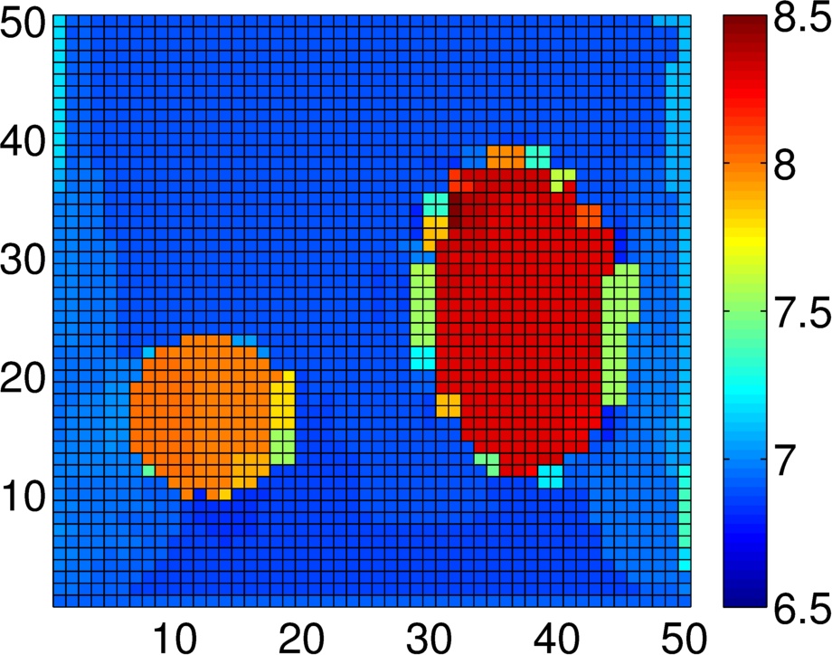


Figure 18 depicts the relative information gain (Section 2.3) for each SNR. The behavior of the information gain depends on the ratio of the prior and the posterior of the variance . As with the previous example, it exhibits a relative quick decay after a small number of reduced coordinates have been added. In Figure 18 shows also the number of forward calls as a function of . As it was observed previously, the effort is expended in the beginning and in all cases the final result is obtained with less than forward calls.


Figure 19 shows the evolution of as a function of the number of forward calls. Figure 20 depicts the corresponding evolution of for and for all three SNR cases.


Finally, Figure 22 depicts basis vectors for each SNR in decreasing order based on the corresponding variance . While similarities are observed the basis vectors are not identical as compared across the three different noise levels reflecting the fact that each dataset is informative along different directions in the space. It is clear however that regions in the vicinity of or on the inclusions exhibit larger posterior variability. As expected the associated variances are larger as the SNR is smaller (i.e. the noise level is higher).
SNR SNR SNR


The aforementioned results for the largest noise case () were validated by employing Importance Sampling as discussed in Section 2.4. The Effective Sample Size (ESS, Equation (57)) was (for ) which suggests a good approximation to the actual posterior is provided by the VB result [93]. More importantly, as it is shown in Figures 23 and 24, the first and second-order statistics of the exact posterior (estimated with Importance Sampling) are very close to the ones computed with the VB approximation.


4 Conclusions
We introduced a novel Variational Bayesian framework for the solution of nonlinear inverse problems and demonstrated its capabilities in problems in elastography. The main advantage of the proposed methodology is the ability to find a much lower-dimensional subspace where a good approximation to the exact posterior can be obtained. The identification of the reduced basis set is founded on a fully Bayesian argumentation that employs Variational approximations to the exact posterior. Information-theoretic criteria have been proposed in order to adaptively identify the the cardinality of the reduced coordinates. The posterior approximations are obtained with a limited number of calls to the forward solver for the computation of the response and its derivatives (in all problems considered fewer than such calls were needed). Furthermore, with the use of Importance Sampling, the (minute) bias in the posterior estimates can be readily corrected and consistent statistics of the exact posterior can be readily estimated.
A possibility that could further reduce the computational effort is the use of forward solvers operating on a hierarchy of resolutions. Starting with the coarsest (and less expensive) model some of the features of the posterior can be obtained with minimal cost and these can be further refined by a smaller number of calls to finer resolution solvers. The resolution of the forward model could also be adaptively altered in regions where the posterior variance appears to be larger. Obtaining efficiently, accurate and fully-Bayesian solutions is a critical step in enabling the use of model-based techniques on a patient-specific basis for medical diagnosis.
A final extension that is currently under exploration is the use of mixtures of Gaussian densities in order to provide better approximations to highly non-Gaussian posteriors or even multi-modal posteriors [84]. Such situations arise frequently in cases where very sparse and/or very noisy data is available and represent the most challenging setting for associated inverse problems [13]. Tools along the aforementioned lines, offer appealing possibilities for identifying multiple low-dimensional subspaces and associated basis vectors which locally provide good posterior approximations and when combined, offer an accurate global solution.
Appendix A Expectation-Maximization for the prior
Due to the analytical unavailability of and its derivatives we employ an Expectation-Maximization scheme which we describe in here for completeness [87, 88]. Proceeding as in Equation (18) i.e. by making use of Jensen’s inequality and an arbitrary distribution we can bound as follows:
| (63) |
The inequality above becomes an equality only when i.e. it is the actual posterior on given . The latter can be readily established from Equations (29) and (31) based on which where:
| (64) |
This suggests a two-step procedure for computing and for each :
- (E-step)
Find from Equation (64)
- (M-step)
References
- [1] G. Johannesson, R. E. Glaser, C. L. Lee, J. J. Nitao, W. G. Hanley, Multi-resolution markovchain-monte-carlo approach for system identification with an application to finite-element models (2005).
- [2] S. Torquato, Random heterogeneous materials: Microstructure and macroscopic properties (2002).
- [3] J. Wang, N. Zabaras, A markov random field model of contamination source identification in porous media flow, International Journal of Heat and Mass Transfer 49 (5) (2006) 939–950.
- [4] C. R. Vogel, Computational methods for inverse problems (2002).
- [5] J. Kaipio, E. Somersalo, Statistical and computational inverse problems (2006).
- [6] R. E. Glaser, G. Johannesson, S. Sengupta, B. Kosovic, S. Carle, G. A. Franz, R. D. Aines, J. J. Nitao, W. G. Hanley, A. L. Ramirez, others, Stochastic engine final report: applying markov chain monte carlo methods with importance sampling to large-scale data-driven simulation (2004).
- [7] I. S. Weir, Fully bayesian reconstructions from single-photon emission computed tomography data, Journal of the American Statistical Association 92 (437) (1997) 49–60.
- [8] B. K. a. Hegstad, O. Henning, others, Uncertainty in production forecasts based on well observations, seismic data, and production history, Spe Journal 6 (4) (2001) 409–424.
- [9] J. Wang, N. Zabaras, Hierarchical bayesian models for inverse problems in heat conduction, Inverse Problems 21 (1) (2005) 183.
- [10] F. Liu, M. J. Bayarri, J. O. Berger, R. Paulo, J. Sacks, A bayesian analysis of the thermal challenge problem, Computer Methods in Applied Mechanics and Engineering 197 (29) (2008) 2457–2466.
- [11] H. K. Lee, D. M. Higdon, Z. Bi, M. A. Ferreira, M. West, Markov random field models for high-dimensional parameters in simulations of fluid flow in porous media, Technometrics 44 (3) (2002) 230–241.
- [12] P. D. Moral, A. Doucet, A. Jasra, Sequential Monte Carlo for Bayesian Computation, 2006.
- [13] P.-S. Koutsourelakis, A multi-resolution, non-parametric, bayesian framework for identification of spatially-varying model parameters, Journal of computational physics 228 (17) (2009) 6184–6211.
- [14] N. Chopin, T. Lelièvre, G. Stoltz, Free energy methods for bayesian inference: efficient exploration of univariate gaussian mixture posteriors, Statistics and Computing 22 (4) (2012) 897–916.
- [15] V. H. Hoang, C. Schwab, A. M. Stuart, Complexity analysis of accelerated MCMC methods for bayesian inversion, Inverse Problems 29 (8) (2013-08) 085010. doi:10.1088/0266-5611/29/8/085010.
- [16] Y. M. Marzouk, H. N. Najm, L. A. Rahn, Stochastic spectral methods for efficient bayesian solution of inverse problems, Journal of Computational Physics 224 (2) (2007-06-10) 560–586. doi:10.1016/j.jcp.2006.10.010.
- [17] I. Bilionis, N. Zabaras, Solution of inverse problems with limited forward solver evaluations: a bayesian perspective, Inverse Problems 30 (1) (2014) 015004.
- [18] A. A. Oberai, N. H. Gokhale, S. Goenezen, P. E. Barbone, T. J. Hall, A. M. Sommer, J. Jiang, Linear and nonlinear elasticity imaging of soft tissue in vivo: demonstration of feasibility, Physics in medicine and biology 54 (5) (2009) 1191.
- [19] N. Ganne-Carrié, M. Ziol, V. de Ledinghen, C. Douvin, P. Marcellin, L. Castera, D. Dhumeaux, J.-C. Trinchet, M. Beaugrand, Accuracy of liver stiffness measurement for the diagnosis of cirrhosis in patients with chronic liver diseases, Hepatology 44 (6) (2006) 1511–1517.
- [20] C. Curtis, S. P. Shah, S.-F. Chin, G. Turashvili, O. M. Rueda, M. J. Dunning, D. Speed, A. G. Lynch, S. Samarajiwa, Y. Yuan, others, The genomic and transcriptomic architecture of 2,000 breast tumours reveals novel subgroups, Nature 486 (7403) (2012) 346–352.
- [21] R. Muthupillai, D. J. Lomas, P. J. Rossman, J. F. Greenleaf, A. Manduca, R. L. Ehman, Magnetic resonance elastography by direct visualization of propagating acoustic strain waves, Science 269 (5232) (1995) 1854–1857.
- [22] A. Sarvazyan, T. J. Hall, Editorial [Hot topic: Elasticity Imaging Part I & II (Guest Editors: Armen Sarvazyan and Timothy J. Hall)], Current Medical Imaging Reviews 7 (4) (2011) 254–254. doi:10.2174/157340511798038620.
- [23] M. M. Doyley, Model-based elastography: a survey of approaches to the inverse elasticity problem, Physics in medicine and biology 57 (3) (2012) R35.
- [24] J. Ophir, I. Cespedes, H. Ponnekanti, Y. Yazdi, X. Li, Elastography: a quantitative method for imaging the elasticity of biological tissues, Ultrasonic imaging 13 (2) (1991) 111–134.
- [25] J. C. Bamber, P. E. Barbone, D. O. Cosgrove, M. M. Doyley, F. G. Fuechsel, P. M. Meaney, N. R. Miller, T. Shiina, F. Tranquart, others, Progress in freehand elastography of the breast, IEICE TRANSACTIONS on Information and Systems 85 (1) (2002) 5–14.
- [26] A. Thomas, T. Fischer, H. Frey, R. Ohlinger, S. Grunwald, J.-U. Blohmer, K.-J. Winzer, S. Weber, G. Kristiansen, B. Ebert, others, Real-time elastography—an advanced method of ultrasound: first results in 108 patients with breast lesions, Ultrasound in obstetrics & gynecology 28 (3) (2006) 335–340.
- [27] K. J. Parker, M. M. Doyley, D. J. Rubens, Imaging the elastic properties of tissue: the 20 year perspective, Physics in medicine and biology 56 (1) (2011) R1.
- [28] P. E. Barbone, C. E. Rivas, I. Harari, U. Albocher, A. A. Oberai, Y. Zhang, Adjoint-weighted variational formulation for the direct solution of inverse problems of general linear elasticity with full interior data, International journal for numerical methods in engineering 81 (13) (2010) 1713–1736.
- [29] A. A. Oberai, N. H. Gokhale, M. M. Doyley, J. C. Bamber, Evaluation of the adjoint equation based algorithm for elasticity imaging, Physics in Medicine and Biology 49 (13) (2004) 2955.
- [30] M. M. Doyley, S. Srinivasan, E. Dimidenko, N. Soni, J. Ophir, Enhancing the performance of model-based elastography by incorporating additional a priori information in the modulus image reconstruction process, Physics in medicine and biology 51 (1) (2006) 95.
- [31] A. Arnold, S. Reichling, O. T. Bruhns, J. Mosler, Efficient computation of the elastography inverse problem by combining variational mesh adaption and a clustering technique, Physics in Medicine and Biology 55 (7) (2010) 2035.
- [32] L. G. Olson, R. D. Throne, Numerical simulation of an inverse method for tumour size and location estimation, Inverse Problems in Science and Engineering 18 (6) (2010) 813–834.
- [33] S. Schleder, L.-M. Dendl, A. Ernstberger, M. Nerlich, P. Hoffstetter, E.-M. Jung, P. Heiss, C. Stroszczynski, A. G. Schreyer, Diagnostic value of a hand-carried ultrasound device for free intra-abdominal fluid and organ lacerations in major trauma patients, Emergency Medicine Journal 30 (3) (2013) e20–e20.
- [34] M. J. Beal, Variational algorithms for approximate Bayesian inference, University of London, 2003.
- [35] C. M. Bishop, Pattern recognition and machine learning, springer, 2006.
- [36] M. I. Jordan, Z. Ghahramani, T. S. Jaakkola, L. K. Saul, An introduction to variational methods for graphical models, Machine learning 37 (2) (1999) 183–233.
- [37] H. Attias, A variational bayesian framework for graphical models, Advances in neural information processing systems 12 (1) (2000) 209–215.
- [38] M. J. Wainwright, M. I. Jordan, Graphical models, exponential families, and variational inference, Foundations and Trends® in Machine Learning 1 (1) (2008) 1–305.
- [39] M. Chappell, A. R. Groves, B. Whitcher, M. W. Woolrich, others, Variational bayesian inference for a nonlinear forward model, Signal Processing, IEEE Transactions on 57 (1) (2009) 223–236.
- [40] B. Jin, J. Zou, Hierarchical bayesian inference for ill-posed problems via variational method, Journal of Computational Physics 229 (19) (2010) 7317–7343.
- [41] T. M. Cover, J. A. Thomas, Elements of information theory, 1991.
- [42] T. A. El Moselhy, Y. M. Marzouk, Bayesian inference with optimal maps, Journal of Computational Physics 231 (23) (2012-10-01) 7815–7850. doi:10.1016/j.jcp.2012.07.022.
- [43] B. A. Olshausen, D. J. Field, Sparse coding with an overcomplete basis set: A strategy employed by V1?, Vision Research 37 (23) (1997) 3311–3325. doi:10.1016/S0042-6989(97)00169-7.
- [44] M. S. Lewicki, T. J. Sejnowski, Learning overcomplete representations, Neural computation 12 (2) (2000) 337–365.
- [45] G. A. Holzapfel, Nonlinear solid mechanics (2000).
- [46] G. T. Mase, R. E. Smelser, G. E. Mase, Continuum mechanics for engineers, CRC press, 2009.
- [47] J. Bonet, A. J. Gil, R. D. Wood, Worked Examples in Nonlinear Continuum Mechanics for Finite Element Analysis, 2012.
- [48] N. H. Gokhale, P. E. Barbone, A. A. Oberai, Solution of the nonlinear elasticity imaging inverse problem: the compressible case, Inverse Problems 24 (4) (2008-08) 045010. doi:10.1088/0266-5611/24/4/045010.
- [49] R. A. Adams, J. J. F. Fournier, Sobolev Spaces, Academic Press.
- [50]
S. Goenezen, P. Barbone, A. A. Oberai,
Solution
of the nonlinear elasticity imaging inverse problem: The incompressible
case, Computer Methods in Applied Mechanics and Engineering 200 (13–16)
(2011) 1406–1420.
doi:10.1016/j.cma.2010.12.018.
URL http://www.sciencedirect.com/science/article/pii/S0045782510003749 - [51] O. C. Zienkiewicz, R. L. Taylor, The finite element method (1977).
- [52] T. J. R. Hughes, T. Hughes, The Finite Element Method: Linear Static and Dynamic Finite Element Analysis, Dover Pubn Inc, 2000-08-16.
- [53] W. E, Principles of Multiscale Modeling, 1st Edition, Cambridge University Press, Cambridge, UK ; New York, 2011.
- [54] C. Schillings, C. Schwab, Sparse, adaptive smolyak quadratures for bayesian inverse problems, Inverse Problems 29 (6) (2013-06) 065011. doi:10.1088/0266-5611/29/6/065011.
- [55] M. B. Giles, N. A. Pierce, An introduction to the adjoint approach to design, Flow, turbulence and combustion 65 (3) (2000) 393–415.
- [56] M. Hinze, R. Pinnau, M. Ulbrich, S. Ulbrich, Optimization with PDE constraints, in: Optimization with Pde Constraints, Vol. 23, 2009, pp. 1–270.
- [57] D. I. Papadimitriou, K. C. Giannakoglou, Direct, adjoint and mixed approaches for the computation of hessian in airfoil design problems, International Journal for Numerical Methods in Fluids 56 (10) (2008) 1929–1943.
- [58]
K. Orginos, A solver for multiple
right hand sides., PoS LATTICE 2007 (2007) 042.
URL https://cds.cern.ch/record/1118470 - [59]
M. H. Gutknecht, T. Schmelzer,
The
block grade of a block Krylov space, Linear Algebra and its Applications
430 (1) (2009) 174–185.
doi:10.1016/j.laa.2008.07.008.
URL http://www.sciencedirect.com/science/article/pii/S0024379508003479 - [60] D. Calvetti, L. Reichel, Tikhonov regularization of large linear problems, BIT Numerical Mathematics 43 (2) (2003) 263–283.
- [61] J. M. Bardsley, Gaussian markov random field priors for inverse problems, Inverse Probl. Imaging 7 (2) (2013) 397–416.
- [62] C. Schwab, A. M. Stuart, Sparse deterministic approximation of bayesian inverse problems, Inverse Problems 28 (4) (2012-04) 045003. doi:10.1088/0266-5611/28/4/045003.
- [63] M. S. Richards, Quantitative three dimensional elasticity imaging (2007).
- [64] H. Rivaz, E. M. Boctor, M. Choti, G. D. Hager, others, Real-time regularized ultrasound elastography, Medical Imaging, IEEE Transactions on 30 (4) (2011) 928–945.
- [65] B. Jin, A variational bayesian method to inverse problems with impulsive noise, Journal of Computational Physics 231 (2) (2012) 423–435.
- [66] S. R. Arridge, J. P. Kaipio, V. Kolehmainen, M. Schweiger, E. Somersalo, T. Tarvainen, M. Vauhkonen, Approximation errors and model reduction with an application in optical diffusion tomography, Inverse Problems 22 (1) (2006) 175.
- [67] J. Kaipio, E. Somersalo, Statistical inverse problems: Discretization, model reduction and inverse crimes, Journal of Computational and Applied Mathematics 198 (2) (2007) 493–504.
- [68] P.-S. Koutsourelakis, A novel bayesian strategy for the identification of spatially varying material properties and model validation: an application to static elastography, International Journal for Numerical Methods in Engineering 91 (3) (2012) 249–268.
- [69] A. Gelman, J. Carlin, H. Stern, D. Rubin, Bayesian Data Analysis, 2nd Edition, Chapman & Hall/CRC, 2003.
- [70] M. Honarvar, R. S. Sahebjavaher, S. E. Salcudean, R. Rohling, Sparsity regularization in dynamic elastography, Physics in medicine and biology 57 (19) (2012) 5909.
- [71] D. J. C. MacKay, Choice of basis for laplace approximation, Machine Learning 33 (1) (1998-10) 77–86. doi:10.1023/A:1007558615313.
- [72] T. Bui-Thanh, C. Burstedde, O. Ghattas, J. Martin, G. Stadler, L. C. Wilcox, Extreme-scale UQ for bayesian inverse problems governed by PDEs, in: Proceedings of the International Conference on High Performance Computing, Networking, Storage and Analysis, IEEE Computer Society Press, 2012, p. 3.
- [73] J. M. Tiangang Cui, Likelihood-informed dimension reduction for nonlinear inverse problems, Inverse Problems 30 (11). doi:10.1088/0266-5611/30/11/114015.
- [74] M. E. Tipping, C. M. Bishop, Probabilistic principal component analysis, Journal of the Royal Statistical Society: Series B (Statistical Methodology) 61 (3) (1999) 611–622.
- [75] N. Dobigeon, J.-Y. Tourneret, Bayesian orthogonal component analysis for sparse representation, Signal Processing, IEEE Transactions on 58 (5) (2010) 2675–2685.
- [76] E. J. Candes, J. Romberg, T. Tao, Robust uncertainty principles: Exact signal reconstruction from highly incomplete frequency information, Ieee Transactions on Information Theory 52 (2) (2006-02) 489–509. doi:10.1109/TIT.2005.862083.
- [77] D. P. Wipf, B. D. Rao, Sparse bayesian learning for basis selection, Ieee Transactions on Signal Processing 52 (8) (2004-08) 2153–2164. doi:10.1109/TSP.2004.831016.
- [78] H. Lee, A. Battle, R. Raina, A. Y. Ng, Efficient sparse coding algorithms, in: Advances in neural information processing systems, 2006, pp. 801–808.
- [79] M. W. Seeger, D. P. Wipf, Variational bayesian inference techniques, Ieee Signal Processing Magazine 27 (6) (2010-11) 81–91. doi:10.1109/MSP.2010.938082.
- [80] T. Bui-Thanh, O. Ghattas, D. Higdon, Adaptive hessian-based nonstationary gaussian process response surface method for probability density approximation with application to bayesian solution of large-scale inverse problems, Siam Journal on Scientific Computing 34 (6) (2012) A2837–A2871. doi:10.1137/110851419.
- [81] R. Peierls, On a Minimum Property of the Free Energy, Physical Review 54 (11) (1938) 918–919. doi:10.1103/PhysRev.54.918.
- [82] R. Muirhead, Aspects of Multivariate Statistical Theory, 1982.
- [83] J. M. Bardsley, D. Calvetti, E. Somersalo, Hierarchical regularization for edge-preserving reconstruction of PET images, Inverse Problems 26 (3) (2010-03) 035010. doi:10.1088/0266-5611/26/3/035010.
- [84] R. A. Choudrey, S. J. Roberts, Variational mixture of bayesian independent component analyzers, Neural Computation 15 (1) (2003-01) 213–252. doi:10.1162/089976603321043766.
- [85] Z. Wen, W. Yin, A feasible method for optimization with orthogonality constraints, Mathematical Programming 142 (1) (2013-12) 397–434. doi:10.1007/s10107-012-0584-1.
- [86] J. Barzilai, J. Borwein, 2-point step size gradient methods, Ima Journal of Numerical Analysis 8 (1) (1988-01) 141–148. doi:10.1093/imanum/8.1.141.
- [87] A. Dempster, N. Laird, D. Rubin, Maximum likelihood from incomplete data via em algorithm, Journal of the Royal Statistical Society Series B-Methodological 39 (1) (1977) 1–38.
- [88] R. M. Neal, G. E. Hinton, A view of the EM algorithm that justifies incremental, sparse, and other variants, in: M. I. Jordan (Ed.), Learning in Graphical Models, Vol. 89, 1998, pp. 355–368.
- [89] L. Itti, P. Baldi, Bayesian surprise attracts human attention, Vision Research 49 (10) (2009-06-02) 1295–1306. doi:10.1016/j.visres.2008.09.007.
- [90]
A. Kong, J. S. Liu, W. H. Wong,
Sequential
Imputations and Bayesian Missing Data Problems, Journal of the
American Statistical Association 89 (425) (1994) 278–288.
doi:10.1080/01621459.1994.10476469.
URL http://www.tandfonline.com/doi/abs/10.1080/01621459.1994.10476469 - [91] C. P. Robert, G. Casella, Monte Carlo Statistical Methods, 2nd Edition, Springer New York, 2004.
- [92] P. Wellman, R. D. Howe, E. Dalton, K. A. Kern, Breast tissue stiffness in compression is correlated to histological diagnosis, Harvard BioRobotics Laboratory Technical Report.
- [93] J. Liu, Monte Carlo Strategies in Scientific Computing, Springer Series in Statistics, Springer, 2001.
- [94] A. Samani, D. Plewes, A method to measure the hyperelastic parameters of ex vivo breast tissue samples, Physics in Medicine and Biology 49 (18) (2004-09-21) 4395–4405. doi:10.1088/0031-9155/49/18/014.
- [95] J. J. O’Hagan, A. Samani, Measurement of the hyperelastic properties of 44 pathological ex vivo breast tissue samples, Physics in Medicine and Biology 54 (8) (2009-04-21) 2557–2569. doi:10.1088/0031-9155/54/8/020.
- [96] M. Mooney, Theory of large elastic deformation, Journal of Applied Physics 11 (1940) 582–592. doi:10.1063/1.1712836.
- [97] R. Rivlin, Large elastic deformations of isotropic materials. further developments of the general theory, Philosophical Transactions of the Royal Society of London Series a-Mathematical and Physical Sciences 241 (835) (1948) 379–397. doi:10.1098/rsta.1948.0024.
- [98] J. Simo, R. Taylor, Quasi-incompressible finite elasticity in principal stretches - continuum basis and numerical algorithms, Computer Methods in Applied Mechanics and Engineering 85 (3) (1991-02) 273–310. doi:10.1016/0045-7825(91)90100-K.
- [99] M. Schöberl, Comparison of different optimization algorithms for nonlinear inverse problems in biomechanics (2013).