VEGAS-SSS. A VST survey of Elliptical Galaxies in the Southern hemisphere: analysis of Small Stellar Systems
Abstract
We present a study of globular clusters (GCs) and other small stellar systems (SSSs) in the field of NGC 3115, observed as part of the ongoing wide-field imaging survey VEGAS, carried out with the 2.6m VST telescope. We use deep and observations of NGC 3115, a well-studied lenticular galaxy with excellent scientific literature. This is fundamental for testing the methodologies, verifying the results, and probing the capabilities of the VEGAS-SSS. Leveraging the large field of view of VST allows us to carry out an accurate study of the distribution and properties of SSSs as a function of galactocentric distance, well beyond galaxy effective radii, in a way not often possible. Our analysis of colours, magnitudes and sizes of SSS candidates confirms the results from the existing studies, some of which carried out with 8-10m class telescopes, and further extends them to previously unreached galactocentric distances, with comparable accuracy. In particular, we find a colour bimodality for the GC population and a de Vaucouleurs profile for the surface density of GCs as for the galaxy light profile. The radial colour gradient of blue and red GCs already found, e.g., by the SLUGGS survey with Subaru and Keck data, is further extended out to the largest galactocentric radii inspected, kpc. In addition, the surface density profiles of blue and red GCs taken separately are well approximated by a density profile, with the fraction of blue GCs being slightly larger at larger radii. We do not find hints of a trend for the red GC subpopulation and for the GC turnover magnitude to vary with radius, but we observe a mag difference in the turnover magnitude of the blue and red GCs subpopulations. Finally, inspecting SSS sizes and colours we obtained a list of ultracompact dwarf galaxies and GC candidates suitable for future spectroscopic follow-up. In conclusion, the present study shows the reliability of the methodologies developed to study SSSs in the field of bright early-type galaxies; and the great potential of the VEGAS survey to produce original results on SSSs science, mainly thanks to the wide-field imaging adopted.
Key Words.
Galaxies: star clusters: general – Galaxies: stellar content – Galaxies: statistics – Galaxies: individual: NGC 3115 – Surveys – Catalogs1 Introduction
The study of the properties of old star clusters in and around galaxies is one of the keystones for understanding the formation and evolution of galaxies (Ashman & Zepf, 1992; Forbes et al., 1997; Côté et al., 1998; Brodie & Strader, 2006; Tonini, 2013). Because of the relative ease to detect them out to large galactocentric distances, and of the lower complexity of their host stellar populations with respect to massive galaxies, star clusters provide an accurate and relatively straightforward tool to unveil the mechanisms that produced the present distribution and evolutionary properties of stars in the host galaxy.
The surroundings of massive galaxies are populated by a zoo of small stellar systems (SSSs hereafter): globular clusters (GCs), extended clusters (ECs), ultra compact dwarfs (UCDs), dwarf spheroidals (dSphs), dwarf ellipticals (dEs), compact ellipticals (cE) etc. (see, e.g., Forbes et al., 2013, and references therein). The characteristic magnitude, colours and half-light radii for some SSS classes are given in Table 1. We emphasize that the distinction between the different SSS types is sometimes not trivial, and somewhat arbitrary, due to the lack of sharp distinction between the classes of SSSs as revealed, for example, by the scaling relations of mass, radius, luminosity, central surface brightness, or velocity dispersion (Drinkwater et al., 2004; Misgeld & Hilker, 2011; Chiboucas et al., 2011; McConnachie, 2012). A natural explanation to the lack of clear class-boundaries is that there is not any. Indeed, the transformation processes occurring in dense environments may cause the disruption or transformation of massive SSSs, littering the galaxy field with the remains of disrupted system: low mass SSSs, stellar streams, etc. (Bassino et al., 1994; West et al., 1995; D’Abrusco et al., 2013; D’Abrusco et al., 2014).
Characterizing the properties of the wealth of SSSs in the potential well of the host galaxy is fundamental for the understanding of their origin, and is an important tool for gauging the growth of the galaxy and, more in general, of cosmic structures.
In this context, the present study is dedicated to the analysis of SSSs in NGC 3115, and is the first of a series aimed at analyzing SSSs in bright early-type galaxies, observed as part of the ongoing imaging VST survey VEGAS (“VST survey of Elliptical Galaxies in the Southern hemisphere”, distributed over many semesters; GTO-INAF program, P.I. Massimo Capaccioli).
An overview of VEGAS, and of its scientific aims, is presented in Capaccioli et al. (2014). At completion, the survey will collect detailed photometric information of bright early-type galaxies, to study the galaxy light distribution out to 15-20 effective radii. These galaxy regions are still almost unexplored in the CCD era, mainly because of the difficulties posed by the reduced detector field-of-view. The coupling of a dedicated survey telescope, the VST (Capaccioli & Schipani, 2011), with a new generation wide-field optical imager, the OmegaCAM (Kuijken, 2011), offers a great opportunity to investigate this issue. Similar studies for the Northern hemisphere are being carried out for the Next Generation Virgo Cluster Survey (Ferrarese et al., 2012, NGVS,), and the MATLAS survey (Duc, 2014).
The specific aims of the VEGAS-SSS series is to study and characterize the properties of the SSSs out to very large galactic radii, taking advantage of VEGAS imaging data. SSSs, especially the GC systems, have been studied for decades, and progress has been limited not so much by telescope collecting area but by field of view and by image quality (both to reduce contamination and to reduce the exposure times). Thus, the use of 8m and even 4m telescopes is not compelling, at least for the photometry. In this paper we show the original achievements possible with wide-field imaging from a 2.6m telescope.
So far, except for the already mentioned ongoing studies from the NGVS and MATLAS surveys, the SSSs field population of only a few galaxies has been analyzed out to large galactocentric radii (Dirsch et al., 2003; Forbes et al., 2011; Usher et al., 2012; Blom et al., 2012), though typical studies did not go much beyond , making difficult a robust estimate of the total background contamination. Taking advantage of the large field of view of the VST we will:
- •
analyze the photometry in and bands for candidates GCs, UCDs, ECs, dSphs, etc. Furthermore, at completion VEGAS will also include data for most of the targets, and for selected galaxies;
- •
study the properties of various SSS populations as a function of galactocentric distance to limits presently unreached;
- •
when possible, characterize the spatial extent of sources, with the specific purpose of increasing the efficiency in distinguishing between the various classes of SSSs;
- •
provide catalogs of SSSs candidates essential for preparing spectroscopic follow-up campaigns based on samples suffering for low or, at least, controlled fore/background contamination. To this aim, VEGAS-SSS data covering the bands, possibly complemented with near-IR photometry, would be particularly efficient (Muñoz et al., 2014).
Here, we present the analysis of the and -band of the field centered on NGC 3115, with the aim of describing the data reduction, the analysis tools and performances of the telescope, and to anticipate the future exploitation of the survey. In particular, the present work will mostly focus on the properties of the GCs system in the galaxy. Throughout the paper we verify the reliability of the methodologies used taking advantage of the large amount of literature data available for NGC 3115 (including results from HST observations and 8-10m class telescopes), and present original results on SSSs topics made possible by the use of the large-format CCD mosaic. Indeed, the case of NGC 3115, an isolated lenticular galaxy, is particularly interesting for testing the procedures used. Because of its proximity, the galaxy and its satellites were targeted by many photometric and spectroscopic studies (Hanes & Harris, 1986; Capaccioli et al., 1987; Kundu & Whitmore, 1998; Puzia et al., 2000; Puzia et al., 2002; Norris et al., 2006; Arnold et al., 2011; Usher et al., 2012). Moreover, it is worth recalling that the GCs system of the galaxy is the first one beyond the Local Group with confirmed bimodal metallicity distribution, as shown by Brodie et al. (2012) from Calcium Triplet analysis, and by Cantiello et al. (2014) using optical to near-IR photometry (Blakeslee et al., 2010; Yoon et al., 2011, see also).
The paper is organized as follows: the next section briefly describes the observations and data reduction procedures. We introduce the data analysis and the full catalog, providing the details of the photometric and morphological study of SSSs candidates, in Section 3. In Section 4, taking advantage of the large field-of-view of the images, we study the properties of the GC population versus galactocentric radius using a statistical background decontamination method. Section 5 is dedicated to the delicate issue of deriving SSS sizes. The final section provides a summary of our main conclusions, and describes the perspectives for the forthcoming VEGAS-SSS studies.
| SSS Class | (mag) | pc | Reference | |
|---|---|---|---|---|
| GC | to | 0.8-1.2 | 2-8 | 3, 6 |
| EC a aa a aa Objects with similar luminosity and size have been also dubbed Faint Fuzzies (Larsen & Brodie, 2000; Peng et al., 2006; Forbes et al., 2013). | to | 1.2 | 8-50 | 6, 7, 13 |
| UCD | to | 0.7-1.3 | 8-100 | 1, 2, 4, 6 |
| dE | to | 0.8-1.2 | 300-1000 | 5 |
| cE | to | 100-500 | 5, 11, 12 | |
| dSph | to | 0.8-1.2 | 50-1500 | 6, 8, 9, 10 |
2 Observations and data reduction
The VST, VLT Survey Telescope, is a wide-field optical imaging telescope with a 2.6-meter aperture, operating from the to the with a corrected field of view of 1 degree by 1 degree. Its single focal plane instrument, OmegaCAM, is a large format (16k 16k pixels) CCD camera with a pixel scale of .
The data reduction, including dither combination, vignetting and exposure correction, astrometric solution and photometric calibration was performed with the VST-Tube pipeline (Grado et al., 2012). Details about the overall data quality can be found in Capaccioli et al. (2014). In particular the FWHM of the PSF varies for across the field of view, and the internal astrometric accuracy is (the with respect to the USNO-B1 catalog is ).
In order to improve the analysis of the spatial extent of the sources in the frame, we restricted our analysis to the imaging data with average PSF FWHM. With this choice the exposure time is reduced by 30% in and in with respect to the total integration time available.
Basic properties for the target and the optical observations are listed in Table 2. The -band image of NGC 3115 is shown in Figure 1.

| Galaxy parameters | |
|---|---|
| RA(J2000)1 | 10h05m14.0s |
| Dec(J2000)1 | -07d43m07s |
| Galaxy Type2 | S0 |
| Distance adopted (Mpc) | 9.4 |
| Absolute -band magnitude2 | -19.9 |
| (km/s, Heliocentric) | 6634 |
| Mean | 0.042 |
| Effective radius | 57 |
| Observations | |
| Filter (median FWHM) | Exposure time (s) |
| () | 2695 |
| () | 1250 |
- 1
Data retrieved from NED, nedwww.ipac.caltech.edu
- 2
Hyperleda leda.univ-lyon1.fr
- 3
Schlegel et al. (1998) with Schlafly & Finkbeiner (2011) recalibration
Given our purpose of studying SSSs, we need to minimize the contamination due to the presence of the light from NGC 3115. To model and subtract the galaxy, we used the ISOPHOTE/ELLIPSE task in IRAF/STSDAS (Jedrzejewski, 1987)22 2 IRAF is distributed by the National Optical Astronomy Observatory, which is operated by the Association of Universities for Research in Astronomy (AURA) under cooperative agreement with the National Science Foundation.. The modeling failed to match the central thick disk region, which implied poor detection of the sources within the inner area33 3 A test with GALFIT (Peng et al., 2002), a further program designed for modeling two-dimensional brightness profiles, also failed the modeling of the central galaxy regions. We also obtained a galaxy-subtracted frame as described in Jordán et al. (2007) and Cantiello et al. (2014, which modeled NGC 3115 from near-IR data). Such method uses the SExtractor spline background derived from the image logarithm, and provided very flat residuals. However, the latter procedure affects badly the shape of slightly extended objects, thus it is not suitable for the purposes of the present study.. However, the central regions of the galaxy have been accurately inspected using a mosaic obtained with the ACS camera on board of the Hubble Space Telescope (Jennings et al., 2014, HST;). The ACS study relies on data with similar wavelength coverage and -band depth with respect to the ones used here. Given the higher resolution of HST data, we do not make any attempt to recover the sources in the central poorly modeled regions along the galaxy major axis.
3 Photometry and size estimates
To produce a complete catalog of all sources present in the VST field of view, we run SExtractor (Bertin & Arnouts, 1996) on the galaxy-model subtracted frame, independently for each filter.
We obtained aperture magnitudes within a 6 pixel diameter aperture ( at OmegaCAM resolution), and applied aperture correction to infinite radius. The aperture correction, derived from the analysis of the curve of growth of bright isolated point-like sources (see Cantiello et al., 2005; Cantiello et al., 2011, for more details), is and mag in and , respectively. For extended sources, i.e. sources spatially more extended than the instrumental FWHM of the PSF (see below), we used the SExtractor Kron-like elliptical aperture magnitude. Finally, the photometric catalogs in the two bands were matched adopting matching radius. The final photometric catalog contained 47000 sources.

Due to the large areal coverage, there is a non-negligible variation of Galactic extinction from one side to the other of the field ( mag). We obtained the local extinctions from the dust maps by Schlegel et al. (1998) and used the reddening factors from Schlafly & Finkbeiner (2011). The final extinction map is shown in Figure 2. All further colours and magnitudes in the paper are corrected for extinction unless otherwise stated. Other details on the photometric properties of the images analyzed (completeness an limiting magnitudes) are given in Appendix A.
The colour magnitude diagram of the full sample of and matched sources is shown in Figure 3 (panel ).

It is very important to emphasize that the selection of SSSs based on one single colour, the , is inherently uncertain, resulting in a catalog with large fractions of contaminating sources (Durrell et al., 2014, foreground stars and background galaxies,). The selection with a further optical color would certainly reduce the fraction of contaminants, especially if band photometry is available. However, a contaminant-free catalog based on optical photometry is basically unattainable. It is useful to highlight, though, that the coupling of optical data with just one near-IR band is very effective in reducing the fraction of contamination to the GC and UCD catalogs to less than % (Muñoz et al., 2014).
To partly overcome the problem of selecting SSSs relying on only one optical colour, one can use statistical decontamination techniques (see Section 4), and/or add a further selection criterion: the physical extent of the source (Table 1). The methodology that we will adopt to derive objects sizes is described below, while the effectiveness and the practical issues in using object sizes as a selection parameter will be discussed in Section 5.
3.1 Size and shape measurements as compactness criterion
As shown in Table 1, if one can estimate the half-light radius of SSSs then the objects shape can be used together with photometric properties to classify the system. However, size measurements can be very challenging, especially with ground-based imaging data. Furthermore, in general one can only measure angular sizes which, to be transformed in linear scale, require the previous knowledge of the object distance. In spite of this, angular sizes and shapes have been estimated for a large sample of SSSs in different environments and with various ground- and space-based telescopes (Larsen, 1999; Larsen & Brodie, 2003; Jordán, 2004; Cantiello et al., 2007; Caso et al., 2013; Puzia et al., 2014, e.g.). In what follows we describe how object sizes have been estimated for objects in the VEGAS-SSS fields.
Given the difficulty posed by the task, to estimate the intrinsic size of a source exceeding some instrumental-dependent size limit, specific tools have been designed and implemented to analyze the light profiles of sources with intrinsic sizes comparable or slightly smaller than the instrumental PSF. For VEGAS-SSS we choose to adopt Ishape44 4 The software can be downloaded at http://baolab.astroduo.org/. For the present work we used the release 0.94.1d. to obtain structural parameters (in particular and the axis ratio ) of SSSs. Ishape is optimized for modeling the light distribution for marginally resolved sources down to 1/10 of the FWHM of the PSF (Larsen, 1999; Larsen & Richtler, 2000). In such context, NGC 3115 is one of the most attractive targets in the survey, being also one of the nearest. At the adopted distance of 9.4 Mpc (Tonry et al., 2001, using the updated calibration zeropoint from Cantiello et al., 2013), and given the FWHM of the images (Table 2), Ishape can be used to determine the physical extent of objects with pc. For the reasons explained in Section 5, we will take into account also objects down to pc. The measurement of source size below the FWHM is particularly demanding in terms of signal-to-noise ratio, SNR, for this reason we have checked that the -band data currently on hand did not provide us of an adequate SNR, hence in the following we will use the estimates derived from the -band only.
Ishape reaches a convergence for of the input sources in the photometric catalog. The size-colour and size-magnitude plots for the sample of sources for which we have structural parameters are shown in Figure 3 (panels and , respectively).
More details on Ishape runs are given in Appendix B.
3.2 Final catalog
| Position | Photometry | Ishape results | ||||||||||||
| ID | RA | Dec | SNR | FWHM | Note a aa a aa 0: source common to both and cataloges without Ishape data, or rejected from the reference and best samples; 1: source in the reference sample; 2: source in the best sample. | |||||||||
| (J2000) | (J2000) | () | (mag) | (mag) | () | (pc) | ||||||||
| (1) | (2) | (3) | (4) | (5) | (6) | (7) | (8) | (9) | (10) | (11) | (12) ) | (13) | (14) | (15) |
| 4 | 151.040149 | -8.155928 | 30.7 | 25.35 0.20 | 0.45 | 24.10 0.23 | 0.56 | 1.250 | 0.053 | … | … | … | … | 0 |
| 6 | 151.484945 | -8.155959 | 28.3 | 24.51 0.09 | 0.70 | 23.91 0.19 | 0.72 | 0.602 | 0.052 | … | … | … | … | 0 |
| 92 | 151.348259 | -8.155089 | 26.3 | 23.97 0.10 | 0.02 | 21.86 0.08 | 0.06 | 2.109 | 0.051 | 18.6 | 0.95 | 12.5 | 0.85 | 0 |
| 93 | 151.091210 | -8.154886 | 29.2 | 24.26 0.12 | 0.39 | 23.05 0.14 | 0.38 | 1.210 | 0.053 | 11.4 | 1.14 | 15.0 | 0.86 | 0 |
| 293 | 151.571415 | -8.153376 | 30.4 | 21.78 0.02 | 0.03 | 21.27 0.04 | 0.03 | 0.502 | 0.051 | 106.7 | 2.49 | 34.8 | 0.97 | 1 |
| 993 | 151.117979 | -8.143415 | 27.9 | 21.86 0.02 | 0.03 | 21.19 0.04 | 0.04 | 0.675 | 0.053 | 94.8 | 1.74 | 22.0 | 0.78 | 1 |
| 1396 | 150.878854 | -8.138160 | 35.8 | 22.37 0.02 | 0.86 | 21.67 0.03 | 0.26 | 0.700 | 0.052 | 64.3 | 0.53 | 6.7 | 0.77 | 2 |
The final catalog resulting from the colour and size/shape criteria is given in Table 3. The catalog contains the full list of sources matched in the and catalogs. For each source, the following parameters are reported: (1) VEGAS-SSS ID, (2) and (3) right ascension and declination (J2000), (4) galactocentric distance, (5) magnitude and error, (6) SExtractor CLASS_STAR parameter in the band , (7) magnitude and error, (8) SExtractor CLASS_STAR parameter in the band ; (9) color; (10) local reddening; (11) signal-to-noise ratio from Ishape; (12) FWHM of the source; (13) effective radius; (14) object minor to major axis ratio (); (15) notes. The absolute value of in pc depends on the distance adopted, thus it is wrong for all unknown contaminating fore/background sources. In Section 5 we will discuss the percentage of contamination expected on the basis of comparison with data from the literature.
4 GC population properties as a function of galactocentric distance: statistical decontamination of the sample
In this section, we analyze the colour and magnitude distribution of SSSs in the field of NGC 3115. In particular, because they dominate the SSS population in the galaxy core, we focus on GCs, making use of statistical decontamination of background sources. To have a better statistics for the background subtraction, we use the entire VEGAS-SSS catalog of and matched sources ( objects), and select as good GCs candidates sources: in the colour range for mag (Faifer et al., 2011; Kartha et al., 2013; Vanderbeke et al., 2014, e.g.); maximum photometric error mag for colour analysis ( mag for magnitude analysis); SExtractor star-galaxy , to avoid contamination from sources that are trivially background galaxies; and mag, i.e. sources brighter than are not taken into account (see below). Thus, for the analysis presented in this section we do not apply any restriction on .
4.1 Background determination
Our approach relies on the assumption that all sources beyond some limiting galactocentric radius, , are foreground or background contaminants, with a uniform spatial distribution over the field. In particular, we adopted (see also Section 5), corresponding to kpc at the distance of the galaxy. Taking as reference the GCs systems in the Milky Way and M 31, we estimate that a fraction of GCs brighter than mag (the approximate 90% limiting magnitude in , see Figure 3, and Appendix A) might still be in the background sample because of their large galactocentric distances kpc. More in detail, the Galaxy has seven GCs, over 157, at 65 kpc (Harris, 1996, 2010 release), only three of them are brighter than the detection limit of our photometric catalog. This implies that, if placed at the distance of NGC 3115, and for random viewing angles, 2% of the MW GCs would be included in the background sample. The GCs catalog of M 31 by Galleti et al. (2004, RBCv5), selected using optical to near-IR colour cuts (Muñoz et al., 2014), contains 447 GC candidates none of which at galactocentric distance larger than 35 kpc. On the other hand, Huxor et al. (2014), using the CFHT/MegaCam data of the PAndAS survey, discovered 59 new GCs at large galactocentric distances in Andromeda: 19 of them would be brighter than our magnitude cut, and with a projected distance larger than 65 kpc from the galaxy center. This corresponds to a fraction the total, assuming a total population of at least 700 GCs (638 from RBCv5, 59 from PAndAS).
Adopting means that of the image is used for the analysis of contamination. The possible future addition of further bands will allow to increase the inner radius for the selection of GCs (more in general, of SSS satellites), allowing to use a smaller fraction of the detector to characterize the contamination.
Under such assumption, the difference between the surface density at galactocentric distance and gives the residual density of sources in NGC 3115, mainly GCs.
We proceeded as follows. We first estimated the surface density of background objects per square arcminute at given colour (or magnitude), , adopting the selection criteria given above, plus the galactocentric distance. Then, the total surface density of objects within elliptical concentric regions, , is estimated using the same criteria on colour (or magnitude), adopting different inner radii, starting from out to , with steps. The geometry of the ellipses, with constant ellipticity and position angle , is assumed according to the results of Capaccioli et al. (2014) (Arnold et al., 2011; Jennings et al., 2014, see also). In the following, is the semi-major axis, if not stated otherwise.
The overdensity of sources at given colors (or magnitude) associated with NGC 3115 is finally estimated as the difference .
4.2 Colour Distribution

The panels in Figure 4 show the density histograms , , and versus colour (from left to right, respectively). In each panel, darker colour refers to regions with smaller inner radii. The histograms after the first innermost radius have been smoothed for sake of clarity. In the first panel of the figure, the density distribution shows the presence of a dip at mag, and two well defined peaks at and mag whose prominence decreases, but does not go to zero, as larger radii are considered.
For background sources (Figure 4, middle panel) the density distribution does not show relevant features, and appears nearly flat over the colour interval shown. As expected, the colour distribution of the difference diagram (Figure 4, right panel) shows two distinct color peaks at all radii.
To investigate the properties of the colour distributions in panel at each given radius, we used the “Gaussian mixture modeling” code (Muratov & Gnedin, 2010, GMM,)55 5 GMM uses the likelihood-ratio test to compare the goodness of fit for double-Gaussians versus a single-Gaussian. For the best-fit double model, it estimates the means and widths of the two components, their separation DD in terms of combined widths, and the kurtosis of the overall distribution. It also provides uncertainties based on bootstrap resampling. In addition, the GMM analysis provides the positions, the relative widths, and the fraction of objects associated with each peak.. More in details, we randomly populated the difference distribution, , with a fixed number of sources (), and then run the GMM code on the repopulated sample.
The results of the GMM run are given in Table 4, where for each it is reported the position of the peak and width of the blue and red distributions, as well as the fraction of GCs associated with each populations (in parentheses). The total fraction, in some cases, does not equal one, because of the presence of a minor very red peak. Figure 5 shows the positions of the blue and red peaks, the standard deviation of each distribution, and the fraction of objects associated with each peak (given by symbol size).
| 2.0 | 0.79 0.18 ( 0.64) | 1.01 0.07 ( 0.30) | 68 |
| 3.0 | 0.78 0.15 ( 0.69) | 1.00 0.06 ( 0.26) | 150 |
| 4.0 | 0.75 0.14 ( 0.64) | 1.02 0.07 ( 0.30) | 204 |
| 5.0 | 0.76 0.14 ( 0.74) | 1.01 0.05 ( 0.19) | 268 |
| 6.0 | 0.76 0.14 ( 0.70) | 1.01 0.05 ( 0.23) | 315 |
| 7.0 | 0.76 0.14 ( 0.70) | 1.02 0.06 ( 0.25) | 364 |
| 8.0 | 0.76 0.13 ( 0.65) | 1.02 0.06 ( 0.29) | 400 |
| 9.0 | 0.75 0.13 ( 0.65) | 1.01 0.06 ( 0.29) | 454 |
| 10.0 | 0.75 0.13 ( 0.65) | 1.00 0.05 ( 0.23) | 518 |
| 11.0 | 0.76 0.13 ( 0.66) | 1.00 0.06 ( 0.24) | 562 |
| 12.0 | 0.75 0.13 ( 0.67) | 1.00 0.06 ( 0.27) | 612 |
| 13.0 | 0.75 0.13 ( 0.69) | 1.00 0.05 ( 0.22) | 661 |
| 14.0 | 0.75 0.14 ( 0.69) | 1.00 0.05 ( 0.21) | 718 |
| 15.0 | 0.75 0.13 ( 0.70) | 1.00 0.05 ( 0.23) | 768 |
| 16.0 | 0.74 0.14 ( 0.69) | 1.01 0.08 ( 0.29) | 833 |
| 17.0 | 0.75 0.14 ( 0.70) | 1.02 0.07 ( 0.28) | 890 |
| 18.0 | 0.75 0.13 ( 0.69) | 1.00 0.05 ( 0.23) | 963 |
| 19.0 | 0.75 0.13 ( 0.69) | 1.00 0.05 ( 0.22) | 1024 |
| 20.0 | 0.75 0.13 ( 0.69) | 1.01 0.06 ( 0.24) | 1086 |
| 21.0 | 0.75 0.14 ( 0.70) | 1.00 0.05 ( 0.22) | 1159 |
| 22.0 | 0.73 0.14 ( 0.66) | 1.01 0.08 ( 0.31) | 1247 |
In the table we also report the number of GC candidates selected according to the selection criteria given above (, column). Using the average surface density of contaminants , and the listed, one can easily derive the expected number of GCs corrected for contamination at each elliptical radius. As an example, the area with roughly corresponds to the ACS area inspected by Jennings et al. (2014), and is expected to contain GCs, to be compared with the 360 candidates found with ACS.
We note that the position of the two peaks and their width are consistent at all radii inspected, and agree very well with the recent similar analysis on the same host galaxy (Faifer et al., 2011; Usher et al., 2012). A closer inspection to the data in Figure 5, and Table 4 reveals the presence of important features. First, a colour- correlation is observed for the blue GC component (Pearson correlation coefficients ), with a mag colour difference between the inner and outer region. There is no, or a very weak, colour-radius correlation for the red GCs (). Furthermore, the fraction of sources in the red sub-population shows a slight but significant decrease with respect to the blue one at large radii. The width of both sequences is relatively stable with radius, with the blue distribution being broader at all radii.
These properties support a scenario where blue GCs are associated with the galaxy halo, while red ones are more centrally concentrated and associated with the bulge stellar component in the galaxy (Kissler-Patig, 1997; Côté et al., 1998; Forte et al., 2005; Liu et al., 2011).
In order to study the population of GCs associated with NGC 3115 excluding the GC contaminants from the neighboring fainter galaxies, we also carried out several tests rejecting all GC candidates within 2-3 from KK 084 and NGC 3115B. The first galaxy, KK 084, is a dSph with center at from NGC 3115, and a non-negligible population of GC candidates, having a specific frequency (Harris & van den Bergh, 1981; Puzia & Sharina, 2008). In spite of the relatively large , the net effect on the properties of the GC system in NGC 3115 is negligible. None of the sources in NGC 3115B falls in the elliptical shaped area of NGC 3115 inspected here.

In Figure 5 we added the data from Arnold et al. (2011), which are part of the SLUGGS survey (Brodie et al., 2014). Gray circles in the figure mark spectroscopic confirmed GCs, green dots mark the running mean for gray dots. We find very good matching between the mean VEGAS-SSS colour obtained with the statistical decontamination approach presented in this section, and the colour of the spectroscopically confirmed GCs.
Arnold et al. (2011) also derived the radial profiles out to combining the spectroscopic sample with a photometric sample, corrected for contamination using “an iterative Monte Carlo scheme” (gray lines in Fig. 5). The matching of the VEGAS-SSS and SLUGGS colour profiles for blue GCs is good at all common radii.
We note that at the colour profiles from Arnold et al. depend mostly on the properties of the photometric sample, thus the transition appearing in both the blue and red GCs profiles at is strongly weighted toward the photometric sample.
For the blue GCs, the difference between the mean from VST and Arnold et al.’s colour of spectroscopically confirmed GCs at is (g-i) mag. For the red GCs component the difference is (g-i) mag.
By coupling the spectroscopic and photometric samples (gray dashed line), Arnold et al. found that the red GCs are on average bluer at larger galactocentric distances as for blue GCs. The presence of a radial trend in the red GCs from SLUGGS data appears mostly beyond , where the photometric sample dominates over the spectroscopic one. Furthermore, the red GCs profile is nearly flat for and , with a mag colour transition in between.
Overall, the radial colour profiles of GCs from the VEGAS-SSS and SLUGGS are consistent if one takes into account the error envelopes, the intrinsic width of the distribution at fixed and the different analysis approaches adopted.
The good matching appears even more strikingly if one takes into account that the data from Arnold et al. (2011), are obtained by coupling band imaging data from Suprime-Cam at the 8.2m Subaru telescope, and spectroscopy from the 10m Keck-II telescope with DEIMOS.
In conclusion, the comparison shown in Figure 5 provides a strong evidence in support of the efficiency of the approach adopted here to analyze the properties of the GC system out to more than galaxy effective radii. It also shows that original results are obtained, even with the photometry in only two passbands, when using the wide-field imaging data from the 2.6m VST telescope.
4.3 Surface density profiles
The radial profiles of the projected surface density for GC candidates are shown in Figure 6. The surface density at each radius is obtained as the difference between the total density of sources with , and the background density.
Taking advantage of the results obtained with GMM on the blue/red GCs, we also analyzed the radial density profiles of the blue/red subpopulations. Dividing the GCs into subpopulations, adopting a sharp blue/red separation at , the radial profile for the red GCs appears steeper than that for the blue GCs. Moreover, both density profiles follow very closely a de Vaucouleurs profile (dotted lines), and both are shallower than the galaxy light profile, showing a behavior similar to other galaxies (Dirsch et al., 2005; Norris et al., 2012, e.g. NGC 4636 and NGC 3923,).


The steeper starlight gradient, compared with GCs density (blue or total GC density), suggests that the GC system of NGC 3115 extends farther than the surface brightness profile of the galaxy halo. This result is consistent with the general picture of the GC system being spatially more extended than the host galaxy (Harris, 1991; Harris et al., 2000; Forbes et al., 2006; Alamo-Martínez et al., 2012; Kartha et al., 2013).
A further feature in Figure 6 is the matching of the density profile for red GCs with the galaxy light profile at (), while the surface density of GCs at smaller radii is slightly lower. Such depletion has already been observed in galaxies brighter than NGC 3115 (Dirsch et al., 2005; Goudfrooij et al., 2007, e.g.), and associated with higher efficiency of GC-disruption mechanisms in the inner galaxy regions (Vesperini, 2001; Goudfrooij et al., 2007, dynamical friction, two-body relaxation and GC tidal shocking,), suggesting that the galaxy has undergone a relatively quiescent evolution, without major star-forming events, which would have increased the inner density of red GCs.
4.4 Luminosity Function: GCLF
Adopting the same approach used for colors in Section 4.2, we analyzed the luminosity function of sources in the field, with the specific purpose of inspecting the GC luminosity function (GCLF) to independently estimate the galaxy distance modulus (Harris, 2001), and further derive the position of the turnover magnitude as a function of galactocentric distance.
Figure 7 shows the surface density distribution obtained as described in previous section, with the difference that in this case we used the total magnitude, instead of colour. The GCLFs derived are corrected for radial-dependent completeness as described in Appendix A. Panel in the figure shows the presence of various local maxima in the density distribution, whereas the distribution of background sources, in panel , has a power law increase with a drop between and mag, due to the completeness limit given by the adopted selection criteria. The density distribution of sources in the host galaxy, shown in panel , reveals the presence of a major peak at mag.
To inspect the presence of a discontinuity in the luminosity function due to the TOM, we adopt a quantitative method introduced by Lee (1993) to identify the position of the RGB Tip in Galactic resolved GCs. The results of such edge-detection method (based on the Sobel filter, see Appendix A) are shown in panel of Figure 7. Although the uncertainties in the surface density, and their propagation in the definition in the edge and second-edge functions are certainly large, the diagrams highlight the presence of an inflection point (edge) and a maximum (edge2) around mag as expected at the TOM (see Figure 1666 6 Inspecting the edge functions two other possible TOM-point candidates are located at and 23.2 mag (see Appendix A). However, both magnitude values are ruled out as TOM peak by the shape of the GCLF.).
In Figure 7, we also show the gaussian GCLF with arbitrary peak normalization, assuming turnover TOM magnitude , with derived from Jordán et al. (2009, eq. 18). A mag tolerance area around is also shown. Adopting the absolute value for the turnover magnitude from the ACS Virgo Cluster Survey for galaxies with , mag, we estimate a distance modulus , in good agreement with the literature distance of the galaxy (Table 2).
Furthermore, thanks again to the large area inspected, we also probe the variation of to large projected galactocentric radii. The data in Figure 7 (panel ) reveal a TOM essentially constant over the spatial scales inspected, as also found in other galaxies (Jordán et al., 2007).
On the basis of the results shown in Figure 7 and in Figure 4, we deduce a low contamination rate in the regions within (first six darker curves in the figures), as the luminosity and colour surface density of contaminants, shown in the central panels, can be one order of magnitude smaller than density in the inner regions. This implies that the rate of contamination of the VEGAS-SSS catalog for NGC 3115 is quite low for the innermost . As an example, the background density at mag is , while the density of sources within is times larger, and gets times larger at .

We further inspected how the TOM differs between red and blue GCs, a test that is not often possible and here feasible thanks to the large area inspected. After dividing the blue/red GCs adopting a sharp colour separation at =0.9, we carried out the analysis described above on the luminosity functions blue and red GCs. The results are shown in Figure 8, where the total luminosity function , the background corrected ones , and the Edge/Edge2 diagrams are shown for the blue and red GCs (upper and lower panels, respectively). Despite the samples adopted are numerically smaller than before, the corrected GCLF still shows the presence of a peak around the same of the total GC population. By estimating the position of the TOM with the Edge functions (right panels in the figure), the interesting point here is that there appear to be a mag offset between the TOM of red and blue GCs, with the red system being fainter. From the point of view of stellar population models, if the GCs mass function is universal across metallicity, the Gaussian mean of the blue GCs is expected to be brighter than that of the red one (Ashman et al., 1995; Di Criscienzo et al., 2006; Jordán et al., 2007). Observationally, our result confirms previous evidences obtained from data with much smaller surface coverage (Whitmore et al., 1995; Puzia et al., 1999; Peng et al., 2009). Further improvements on this will be allowed by the analysis of new galaxies in the VEGAS-SSS sample, with the possible inclusion of and band data in the SSSs selection process.
As a final comment, we highlight that the depth, in terms of absolute magnitude, and the image quality for the other galaxies in the VEGAS sample will be similar to the one inspected here, thus we expect that using the tools presented here77 7 Apart from the size/shape inspection, that will hardly be possible for GCs in distant galaxies, but doable for the UCDs., we will reliably analyze the colour distributions and study GCs luminosity function for all other targeted galaxies out to unreached galaxy effective radii. Moreover, for objects at larger distances the background decontamination methods described in this section will likely be more effective because of the larger galactocentric distances inspected.


5 Object sizes: comparison with literature and analysis
In this section we present a detailed analysis of the properties of the SSS in the field of NGC 3115, and concentrate on the sample of objects with estimates from Ishape.
5.1 Comparing VEGAS-SSS and HST/ACS derived photometry and sizes
As already mentioned, using the photometry and size measurement tools described in the Section §3.1, we ended up with a catalog containing 30000 sources. We compared our measurements with the estimates by Jennings et al. (2014), based on ACS/HST and observations. At the distance of the galaxy, all sources in the field of NGC 3115 with pc appear resolved at the pixel resolution of the ACS. Thus we assume the measured from ACS data as best representing the true distribution of for the GCs in the galaxy, within the limited common area.
The matching of the GCs list from Jennings et al. (2014) with the VST catalog (using radius) contains a list of of the 360 candidates88 8 We found a systematic shift in RA, . In our analysis we applied the correction to ACS data.. Nearly of the unmatched sources are GCs located in the central galaxy regions, where we do not model and subtract the galaxy light profile. The remaining of missing objects are faint sources, undetected in the shallower image, or objects blended with bright neighbors. The number of missed sources beyond the central regions drops to if the sole band catalog is considered (again faint or blended sources). The comparisons of -band ACS and VEGAS-SSS photometry, shown in Figure 9 versus magnitude and colour, reveals very good agreement. In the figure, the full ACS catalog (Z. Jennings, private communication) and the sole GCs sample are considered separately. For sake of homogeneity the comparison with ACS is done using constant extinction. The large scatter for the full sample (left panels) is due to the presence of extended background sources, whose aperture magnitude does not represent a good estimate for the total magnitude, neither for ACS nor for VEGAS-SSS. Comparison of photometry for the sole GCs (right panels in the figure) indicates negligible mean residual difference, both in magnitude and colour.
We also compared the estimates from VEGAS-SSS with the ACS ones. In the comparison one must note that the list of SSS candidates is not contaminant free in either catalogs, as it includes background sources whose (linear) estimates are wrong because they are derived according to the distance of the galaxy. In spite of this, the ACS VEGAS-SSS comparison is still valid since the same distance modulus is assumed in both analysis. Moreover, it should also be noted that the size estimates are not equally good for the full sample of objects measured. Thus, we define a reference sample of VEGAS-SSS candidates with reliable structural and photometric parameters, adopting the following criteria derived on the basis of the comparison with ACS photometry and objects shape:
- •
Ishape signal-to-noise ratio SNR (Larsen, 1999);
- •
total relative error on 30%;
- •
for each source where the iteration to derive was successful, Ishape provides a cutout of the image with the object analyzed, the model brightness profile, the residuals between them, and the weighting map (Larsen, 1999). To reject sources with large residuals (see Appendix C, Figure 22), but otherwise good SNR and FWHM error, after various experiments where we inspected the statistical properties of the residual cutouts, we chose a limit of for good candidates. This criterion applies for objects with contaminating neighbors or structures not accounted for by the previous criteria;
- •
as in Section §4 we adopted colour range mag both for GCs and UCDs;
- •
maximum photometric uncertainty mag;
- •
axial ratio, . (van den Bergh & Morbey, 1984; Blakeslee & Barber DeGraaff, 2008; Cantiello et al., 2009).
Figure 10 shows the VEGAS-SSS to ACS size comparison for the full and reference samples. A first evidence is the “coma” shaped distribution of data. Such behavior highlights the expected lack of accuracy of Ishape for objects with effective radii below 1/10 the FWHM, i.e. pc at the distance of the galaxy.
If only sources in the reference sample and with pc are used (black filled circles in Figure 10, left panels), the median ratio of ACS and VEGAS-SSS s is 1.02, while ( derived from the median absolute deviation) of the ratio is . Thus, for the 29 matched objects in the reference sample, the median and standard deviation of the mean are , providing a satisfactory agreement for the ACS and VEGAS-SSS samples when limited to the reference sample. Nevertheless, we must highlight that the estimates for single objects can differ up to a factor 5 even for pc. Further details on the differences between ACS and VEGAS-SSS size estimates for extended objects are given in Appendix C.
However, for the typical VEGAS target the selection will only rely on measurements from VST images. Right panels of Figure 10 show the same data of left panels, using the values for the selection instead of . The ACS to VEGAS-SSS comparison worsens, as the to mean ratio and standard deviation of the mean are 0.570.06. It is interesting to note that, taking as lower limit pc, we obtain (, 46 objects). This suggests that even though the nominal limit for Ishape is 1/10 the FWHM, or pc at the distance of NGC 3115, the tool allows to separate stars from extended sources down to 2 pc.

To further inspect the issue, Figure 11 shows the distributions for: the full list of matched sources from ACS and VEGAS-SSS (left panel, ACS data in gray, VST data with thick black line), objects in the reference sample selected using pc (middle panel), and objects in the reference sample selected using pc (right panel). The ACS and VEGAS-SSS distributions appear quite similar in middle panel (case ). The distributions based on VEGAS-SSS half-light radii (right panel, case shows a shift, with VEGAS-SSS radii being on average larger, and missing the peak at pc seen in the ACS data. This behavior is due to the sources more compact than 3.5 pc, which are scattered over the entire 3.5-20 pc interval when estimates from VST are used. In particular, the list of common SSS candidates in the reference sample goes from 28, with the selection based on the ACS radii, to 39 with the selection from VST data. On such basis, we estimate that for values of pc the reference sample contains objects with unreliable effective radii, spread over the entire distribution. Needless to say that the sample of matched objects with high quality VEGAS-SSS sizes is relatively small (28 or 39, depending on the selection), thus making hard to generalize the results of the comparison over the entire VST field of view.
Finally, with the aim of deriving a catalog of GC candidates from the sole VST data, and estimating the contamination taking as reference the ACS GCs list, we carried out the following blind test. We adopted the selection criteria given at the beginning of this section, with the additional requirement that GC candidates must have pc (we adopted the same used for GC by Jennings et al., 2014, for ACS data), and matched such VEGAS-SSS list to the sample of GC candidates from ACS. The results is that of the candidates ( over ) are not present in the GC list from ACS99 9 The result is not much sensitive to the particular choices of Ishape input parameters (see Appendix B, Figure 18).. In contrast, adopting as lower limit pc, the number of matching sources is and the contamination is nearly doubled. In other words, the test points out that the results from Ishape allow to distinguish between compact and extended sources down to pc, although the exact value of the effective radius is reliable only above pc.


In conclusion, using the reference sample obtained from the
coupling of photometric and spatial extent properties, the present
VEGAS-SSS catalog can be used to:
obtain a list of GC candidates,
selected in the range , with an expected
contamination of , poorly populated because of the narrow
selection adopted. The number of GC candidates over the entire area
inspected, (or kpc
kpc), selected on the given photometric and size criteria
is . However, for radii below 3.5 pc, the
are only used as an effective binary selection criterion
(i.e. () meaning extended (point-like) source), as this
limit is smaller than the nominal limit of the tool;
a
catalog of extended objects with pc, having a
contamination of objects with unreliable estimates.
5.2 GC and UCD population properties based on colour and size selection criteria
Figure 12 shows the size versus magnitude diagram obtained using the reference sample, i.e. with the selection criteria described in the previous section, and adopting for all objects in the field the same distance modulus. In the right panel, we plotted only SSSs at galactocentric distance , corresponding to kpc at the distance of NGC 3115. The approximate regions for GCs, UCDs, extended clusters (ECs), dwarf spheroidal (dSphs), dwarf ellipticals (dEs) and compact ellipticals (cEs) are shown and labeled (Brodie et al., 2011; Brüns & Kroupa, 2012, yellow regions; mean loci are taken from).
From Figure 12 (left panel), we find that a large fraction of selected objects in the reference sample falls within the avoidance region at mag and pc (Forbes et al., 2013). The situation does not seem to improve much even if only sources in the reference sample and with SNR (best sample hereafter, red circles in the figure) are considered. On the other hand, the number of sources in the avoidance area is lowered if only sources within are taken (Figure 12, right panel), but still significantly large. Moreover, we must highlight the large number of UCD candidates even for the best sample and for sources ().
In spite of the results by Forbes et al. (2013), who find that the avoidance zone is the result of a selection bias and confirmed the presence of various SSSs within the region, a large fraction of sources in the avoidance area are likely background galaxies (some of which are recognizable by eye). As shown by the arrow in Figure 12, in fact, a background source should move toward larger absolute radii and brighter when larger distance moduli are considered.
In right panel of Figure 12, we also plotted the GCs (green circles) and UCDs (squares) data from Jennings et al. (2014). The spectroscopically confirmed GCs and UCDs from Arnold et al. (2011) are plotted as solid symbols. Two interesting elements here are the nice overlap of the overdensity region for spectroscopically confirmed GCs and VEGAS-SSS selections, at and pc, and the presence of UCDs from the ACS sample outside the region where they typically occur. Three UCD candidates from the ACS sample, in fact, lie at mag and pc, i.e. within the zone of avoidance (if any). Two other UCDs have mag and pc, typically associated with the EC region (see also the discussion in Appendix C). This clearly shows that the distinction between the different SSS types is not trivial, and sometimes contains elements of arbitrariness.
To further inspect the issue, we analyzed the surface density distribution of sources versus galactocentric radius, and versus . Figure 13 shows the radial surface density distribution for the reference and best samples (black and red histograms in panel , respectively), for GC candidates (, panel ), and for UCD candidates (, panel )1010 10 To estimate the density of sources, the effective area coverage in each annulus is corrected for the annular area outside the image and for the central uninspected regions (dashed histograms show the uncorrected distributions). Poisson statistics is adopted to estimate the errors.. The gray lines in the figure show the profile assuming a constant background, obtained from the flat region at galactocentric radius . In each panel we also report the total number of objects selected for the reference and best sample (the latter in parentheses). The surface density for the sample with no selection on sizes (panel ) shows an obvious correlation with , and a flattening at , suggesting that sources beyond this radius are most likely background galaxies or foreground stars. The radial density profile for GC candidates follows a de Vaucouleurs density profile out to , as for the galaxy light, providing further proof to the actual membership of the objects selected to the GCs population, and supporting the role of the object-size analysis carried out here. However, one must not neglect the presence of a fraction of background sources. For what concerns the distribution of objects with UCD-like radii, the reference sample does not show a tendency for a radial trend. The result is not surprising, given the small number of expected UCD-candidates and the large fraction of contaminants. It is noteworthy, though, that the UCDs in the best sample show hints of a radial trend.
By integrating the fitted de Vaucouleurs density profiles, from zero to for both GC and UCD density profiles, after subtracting the total number of background sources we find for the reference (best) GC sample (), and for the best UCD sample . The comparison of these numbers, in particular for the GCs, with the numbers in Figure 12 (right panel) confirm our previous results that the contamination for the reference GC sample is , and also indicates that the best sample suffers from very small contamination. The numbers are quite different for UCDs, given the higher confusion with extended background sources. In such case, the coupling with data in other passbands will greatly reduce the contamination.
Figure 14 shows the distributions for the reference and best samples, normalized to the area inspected: full detector area, objects within the area, objects outside , and the difference between latters (from panel to panel , respectively).
The reference sample over the entire VST area (upper panel), shows slightly increasing surface density for increasing up to 50 pc. While the distribution for the best sample is rather flat. The differences of the surface density for objects within or in the outside area, shown in panels and of Figure 14, are quite obvious, especially for the over-density of objects with GC-like radii, . Because of the contamination, the density of sources with GC-like radii is non-zero in the outer radius (panel ). This is in part due to the expected fraction of galaxy GCs that might lie at large galactocentric distances (see Section 4), while most of the contribution comes from background contamination. Indeed, the mean density of objects with at radii (panel ) is 30% the one at (panel ). This result confirms our previous estimate of the fraction of contamination for the colour and size selected reference sample. Furthermore, we note that the density in the background region is 15% the one in the inner regions for the best sample.


The differences between inner and outer density are better seen in panel of Figure 14, where versus is shown. Here, the surface density of sources with pc is consistent with zero. More in details, the distribution for the reference sample (black histogram), is generally consistent with zero density from 50 pc (with some possible candidates at pc), and for pc, while for the best sample various regions are compatible with zero density (e.g pc, pc, and pc). These results, imply that the surface density of objects with such values is constant over the inspected area, as would be expected from a uniform background contamination. In other words, panel suggests that the majority of sources falling in the zone of avoidance (Figure 12) are background galaxies. Second, the over-abundance of sources with having GCs-like radii appears clearly both for the reference and best samples. Furthermore, for the reference sample, we find a positive density of sources around the characteristic values of UCDs (between 10 and 40 pc), which confirms the membership to this class for some of the selected objects. Such over-density, though, is weaker for the best sample, and possibly consistent with zero in some cases.
6 Summary
In this paper we presented the first results of the VEGAS survey for the specific science case of small stellar systems, SSSs. We described the methodology for the photometry and the size analysis of SSS candidates in the field of NGC 3115, a well studied lenticular galaxy, and showed the potential of the survey in providing original results on SSS-related science.
The VEGAS survey will collect the deep and imaging of bright ellipticals in the Southern hemisphere, possibly complemented with for most of the targets, and also with band observations for selected galaxies. One of the great advantages of VEGAS-SSS is the use of wide field imaging, square degree, which allows to study the properties of SSSs out to very large galactocentric distances, with an accurate characterization of the background contaminating objects. For the specific case of NGC 3115 we inspected the properties of SSSs out to , i.e. more than twenty times the effective radius of the galaxy.
We first analyzed the properties of the GCs system. Being the population of SSSs numerically most abundant in the galaxy, GCs properties can be derived using the sole photometric information, colour and magnitudes, by comparing the surface density of sources in the inner galaxy regions with the density in the outer regions. Our results can be roughly divided into two groups: results that repeat previous analysis, giving us the chance to confirm the reliability of this study; new results allowed by the use of the wide-field imaging. In the first group we include:
- •
the GCs have a bimodal distribution with peaks at and mag;
- •
red GCs are more centrally concentrated than blue GCs;
- •
as for the galaxy light, the radial density of GCs follows a de Vaucouleurs profile, but with a shallower slope.
- •
the turnover magnitude of the -band GCLF, , coupled with the calibration from the ACSVCS survey, implies a distance modulus in good agreement with the literature.
Such achievements support the results of previous studies, some of which carried out with 8-10m class telescopes, and are further complemented by the following compelling results:
- •
the colour bimodality extends to more than galaxy effective radii;
- •
the blue GCs show a tendency towards bluer colour at larger galactocentric radii , while red GCs seem to have a nearly constant colour with ;
- •
the galaxy light has a steeper density profile than the GCs, whether the blue or total fractions of GCs is taken into account;
- •
the slope of the surface density profile for red GCs at matches with that for the galaxy light, while a red GCs overdensity appears in the inner galaxy regions;
- •
the ratio of blue to red clusters shows a trend with , with the fraction of blue GCs being slightly larger at larger radii;
- •
by analyzing separately the blue and red GCs we find a mag, with the blue TOM being brighter;
- •
we do not find an obvious dependence of with .
Both the colour and luminosity properties obtained are consistent with similar existing studies of the GC system in other early-type galaxies.
The presence of a bimodal GC system, with blue GCs more extended than
the galaxy stellar light, and a deficiency of red GCs in the inner
regions, have already been observed in other early-type galaxies
brighter than NGC 3115, and support a scenario where blue GCs are
associated with the galaxy halo, while red ones are more centrally
concentrated and associated with the bulge stellar component in the
galaxy. The overall observed properties might suggest that the galaxy has
undergone a relatively quiescent evolution, without major star-forming
events.
Adding the spatial extent of the sources to the colour
information gives a further criterion for selecting SSSs, in particular
GCs and UCDs. We used Ishape to determine the effective
radius of slightly extended objects in the field. By comparing
our estimates for the objects in the reference sample with the
ones in the literature, obtained from ACS data, we find on average
satisfactory agreement. However, the estimates for single
objects can differ up to a factor 5 between ACS and
VEGAS-SSS. Furthermore, the result is sensitive to the estimate taken
as reference (ACS or VEGAS-SSS), because of the contamination of the VEGAS-SSS
sample. The various comparisons with the literature and with
inner/outer galaxy regions suggest that the level of fore/background
contamination of our reference sample is 30%, possibly
reduced to one half for the (poorer) best sample. Future
studies with new VEGAS-SSS and band data will be used to further
constrain the properties of other, less populated classes of SSSs,
like cEs, in the field of NGC 3115.
In spite of the large uncertainties posed by the estimate of ,
the results obtained are encouraging, suggesting that similar analysis
could be successfully carried out for the other targets in the
survey. Although, at larger distances, the study of sizes will be
limited to the most extended SSSs (UCDs, cEs), excluding the GCs
component for most of the targets beyond Mpc distance.
The results of this work, on one hand confirm the existing
studies, thus support the validity of the analysis scheme developed
here using data from the 2.6m VST telescope. On the other hand they
provide new and independent results - especially for what concerns
the GCs properties out to the previously unreached galactocentric
distance of kpc - showing the great potential for future
applications to other VEGAS targets, in particular for the part of
the sky not accessible to similar facilities.
As a final remark, we highlight that, at survey completion, for
most of the VEGAS targets observations in at least one more
passband other than and will be available. The selection of
SSSs with a further optical color would certainly reduce the percentage
of contaminants, especially if band photometry is
included. However, a contamination free catalog based on purely
optical photometry is basically unattainable. Since the coupling of
optical data with just one near-IR band is very effective in reducing
the fraction of contaminants to the GC and UCD populations to
%, the VEGAS-SSS catalogs will be perfectly suited to be
complemented with single-band near-IR imaging (e.g. with a large
format near-IR imager like VISTA), to define the most complete and
clean SSS catalogs possible, essential for, e.g., future spectroscopic
follow-up.
Acknowledgements.
The optical imaging is collected at the VLT Survey Telescope using the Italian INAF Guaranteed Time Observations. The data reduction for this work was carried out with the computational infrastructures of the VST Center at Naples (VSTceN). We gratefully acknowledge INAF for financial support to the VSTceN. Part of this work was supported by PRIN-INAF 2011 (P.I.: G. Marconi), FIRB-MIUR 2008 (P.I. G. Imbriani), PRIN-INAF 2011 (P.I.: A. Grado). M.P. acknowledges finical support from project FARO 2011 from the University of Naples Federico II. D.A.F. thanks the ARC for financial support via DP130100388. We are grateful to John P. Blakeslee, and Zach Jennings for useful discussions related to this work. This research has made use of the NASA/IPAC Extragalactic Data-base (NED) which is operated by the Jet Propulsion Laboratory, California Institute of Technology, under contract with the National Aeronautics and Space Administration. This research has also made use of the SIMBAD database, operated at CDS, Strasbourg, France, and of the HyperLeda database (http://leda.univ-lyon1.fr).References
- Alamo-Martínez et al. (2012) Alamo-Martínez, K. A., West, M. J., Blakeslee, J. P., et al. 2012, A&A, 546, A15
- Arnold et al. (2011) Arnold, J. A., Romanowsky, A. J., Brodie, J. P., et al. 2011, ApJ, 736, L26
- Ashman et al. (1995) Ashman, K. M., Conti, A., & Zepf, S. E. 1995, AJ, 110, 1164
- Ashman & Zepf (1992) Ashman, K. M. & Zepf, S. E. 1992, ApJ, 384, 50
- Bassino et al. (1994) Bassino, L. P., Muzzio, J. C., & Rabolli, M. 1994, ApJ, 431, 634
- Bernstein et al. (2002) Bernstein, R. A., Freedman, W. L., & Madore, B. F. 2002, ApJ, 571, 107
- Bertin & Arnouts (1996) Bertin, E. & Arnouts, S. 1996, A&AS, 117, 393
- Blakeslee & Barber DeGraaff (2008) Blakeslee, J. P. & Barber DeGraaff, R. 2008, AJ, 136, 2295
- Blakeslee et al. (2010) Blakeslee, J. P., Cantiello, M., & Peng, E. W. 2010, ApJ, 710, 51
- Blom et al. (2012) Blom, C., Spitler, L. R., & Forbes, D. A. 2012, MNRAS, 420, 37
- Brodie et al. (2011) Brodie, J. P., Romanowsky, A. J., Strader, J., & Forbes, D. A. 2011, AJ, 142, 199
- Brodie et al. (2014) Brodie, J. P., Romanowsky, A. J., Strader, J., et al. 2014, ArXiv e-prints
- Brodie & Strader (2006) Brodie, J. P. & Strader, J. 2006, ARA&A, 44, 193
- Brodie et al. (2012) Brodie, J. P., Usher, C., Conroy, C., et al. 2012, ApJ, 759, L33
- Brüns & Kroupa (2012) Brüns, R. C. & Kroupa, P. 2012, A&A, 547, A65
- Cantiello et al. (2007) Cantiello, M., Blakeslee, J. P., & Raimondo, G. 2007, ApJ, 668, 209
- Cantiello et al. (2014) Cantiello, M., Blakeslee, J. P., Raimondo, G., et al. 2014, A&A, 564, L3
- Cantiello et al. (2005) Cantiello, M., Blakeslee, J. P., Raimondo, G., et al. 2005, ApJ, 634, 239
- Cantiello et al. (2009) Cantiello, M., Brocato, E., & Blakeslee, J. P. 2009, A&A, 503, 87
- Cantiello et al. (2011) Cantiello, M., Brocato, E., & Capaccioli, M. 2011, A&A, 534, A35
- Capaccioli et al. (1987) Capaccioli, M., Held, E. V., & Nieto, J.-L. 1987, AJ, 94, 1519
- Capaccioli & Schipani (2011) Capaccioli, M. & Schipani, P. 2011, The Messenger, 146, 2
- Capaccioli et al. (2014) Capaccioli et al., M. 2014, in preparation
- Caso et al. (2013) Caso, J. P., Bassino, L. P., Richtler, T., Smith Castelli, A. V., & Faifer, F. R. 2013, MNRAS, 430, 1088
- Chiboucas et al. (2011) Chiboucas, K., Tully, R. B., Marzke, R. O., et al. 2011, ApJ, 737, 86
- Côté et al. (1998) Côté, P., Marzke, R. O., & West, M. J. 1998, ApJ, 501, 554
- D’Abrusco et al. (2014) D’Abrusco, R., Fabbiano, G., Mineo, S., et al. 2014, ApJ, 783, 18
- D’Abrusco et al. (2013) D’Abrusco, R., Fabbiano, G., Strader, J., et al. 2013, ApJ, 773, 87
- Di Criscienzo et al. (2006) Di Criscienzo, M., Caputo, F., Marconi, M., & Musella, I. 2006, MNRAS, 365, 1357
- Dirsch et al. (2003) Dirsch, B., Richtler, T., Geisler, D., et al. 2003, AJ, 125, 1908
- Dirsch et al. (2005) Dirsch, B., Schuberth, Y., & Richtler, T. 2005, A&A, 433, 43
- Drinkwater et al. (2004) Drinkwater, M. J., Gregg, M. D., Couch, W. J., et al. 2004, PASA, 21, 375
- Duc (2014) Duc, P.-A. 2014, ArXiv e-prints
- Durrell et al. (2014) Durrell, P. R., Côté, P., Peng, E. W., et al. 2014, ArXiv e-prints
- Faifer et al. (2011) Faifer, F. R., Forte, J. C., Norris, M. A., et al. 2011, MNRAS, 416, 155
- Ferrarese et al. (2012) Ferrarese, L., Côté, P., Cuillandre, J.-C., et al. 2012, ApJS, 200, 4
- Forbes et al. (1997) Forbes, D. A., Brodie, J. P., & Grillmair, C. J. 1997, AJ, 113, 1652
- Forbes et al. (2013) Forbes, D. A., Pota, V., Usher, C., et al. 2013, MNRAS, 435, L6
- Forbes et al. (2006) Forbes, D. A., Sánchez-Blázquez, P., Phan, A. T. T., et al. 2006, MNRAS, 366, 1230
- Forbes et al. (2011) Forbes, D. A., Spitler, L. R., Strader, J., et al. 2011, MNRAS, 413, 2943
- Forte et al. (2005) Forte, J. C., Faifer, F., & Geisler, D. 2005, MNRAS, 357, 56
- Galleti et al. (2004) Galleti, S., Federici, L., Bellazzini, M., Fusi Pecci, F., & Macrina, S. 2004, A&A, 416, 917
- Goudfrooij et al. (2007) Goudfrooij, P., Schweizer, F., Gilmore, D., & Whitmore, B. C. 2007, AJ, 133, 2737
- Grado et al. (2012) Grado, A., Capaccioli, M., Limatola, L., & Getman, F. 2012, Memorie della Societa Astronomica Italiana Supplementi, 19, 362
- Hanes & Harris (1986) Hanes, D. A. & Harris, W. E. 1986, ApJ, 304, 599
- Harris (1991) Harris, W. E. 1991, ARA&A, 29, 543
- Harris (1996) Harris, W. E. 1996, AJ, 112, 1487
- Harris (2001) Harris, W. E. 2001, in Saas-Fee Advanced Course 28: Star Clusters
- Harris et al. (2000) Harris, W. E., Kavelaars, J. J., Hanes, D. A., Hesser, J. E., & Pritchet, C. J. 2000, ApJ, 533, 137
- Harris & van den Bergh (1981) Harris, W. E. & van den Bergh, S. 1981, AJ, 86, 1627
- Huxor et al. (2014) Huxor, A. P., Mackey, A. D., Ferguson, A. M. N., et al. 2014, MNRAS, 442, 2165
- Huxor et al. (2005) Huxor, A. P., Tanvir, N. R., Irwin, M. J., et al. 2005, MNRAS, 360, 1007
- Jedrzejewski (1987) Jedrzejewski, R. I. 1987, MNRAS, 226, 747
- Jennings et al. (2014) Jennings, Z. G., Strader, J., Romanowsky, A. J., et al. 2014, AJ, 148, 32
- Jordán (2004) Jordán, A. 2004, ApJ, 613, L117
- Jordán et al. (2007) Jordán, A., McLaughlin, D. E., Côté, P., et al. 2007, ApJS, 171, 101
- Jordán et al. (2009) Jordán, A., Peng, E. W., Blakeslee, J. P., et al. 2009, ApJS, 180, 54
- Karachentsev et al. (2001) Karachentsev, I. D., Sharina, M. E., Dolphin, A. E., et al. 2001, A&A, 375, 359
- Kartha et al. (2013) Kartha, S. S., Forbes, D. A., Spitler, L. R., et al. 2013, MNRAS
- King (1962) King, I. 1962, AJ, 67, 471
- Kissler-Patig (1997) Kissler-Patig, M. 1997, A&A, 319, 83
- Kuijken (2011) Kuijken, K. 2011, The Messenger, 146, 8
- Kundu & Whitmore (1998) Kundu, A. & Whitmore, B. C. 1998, AJ, 116, 2841
- La Barbera et al. (2008) La Barbera, F., de Carvalho, R. R., Kohl-Moreira, J. L., et al. 2008, PASP, 120, 681
- Larsen (1999) Larsen, S. S. 1999, A&AS, 139, 393
- Larsen & Brodie (2000) Larsen, S. S. & Brodie, J. P. 2000, AJ, 120, 2938
- Larsen & Brodie (2003) Larsen, S. S. & Brodie, J. P. 2003, ApJ, 593, 340
- Larsen & Richtler (2000) Larsen, S. S. & Richtler, T. 2000, A&A, 354, 836
- Lee (1993) Lee, M. G. 1993, ApJ, 408, 409
- Liu et al. (2011) Liu, C., Peng, E. W., Jordán, A., et al. 2011, ApJ, 728, 116
- Madrid (2011) Madrid, J. P. 2011, ApJ, 737, L13
- McConnachie (2012) McConnachie, A. W. 2012, AJ, 144, 4
- Mieske et al. (2006) Mieske, S., Hilker, M., Infante, L., & Jordán, A. 2006, AJ, 131, 2442
- Mieske et al. (2012) Mieske, S., Hilker, M., & Misgeld, I. 2012, A&A, 537, A3
- Misgeld & Hilker (2011) Misgeld, I. & Hilker, M. 2011, MNRAS, 414, 3699
- Misgeld et al. (2009) Misgeld, I., Hilker, M., & Mieske, S. 2009, A&A, 496, 683
- Muñoz et al. (2014) Muñoz, R. P., Puzia, T. H., Lançon, A., et al. 2014, ApJS, 210, 4
- Muratov & Gnedin (2010) Muratov, A. L. & Gnedin, O. Y. 2010, ApJ, 718, 1266
- Norris et al. (2012) Norris, M. A., Gebhardt, K., Sharples, R. M., et al. 2012, MNRAS, 421, 1485
- Norris et al. (2006) Norris, M. A., Sharples, R. M., & Kuntschner, H. 2006, MNRAS, 367, 815
- Peng et al. (2006) Peng, E. W., Côté, P., Jordán, A., et al. 2006, ApJ, 639, 838
- Peng et al. (2002) Peng, E. W., Ford, H. C., Freeman, K. C., & White, R. L. 2002, AJ, 124, 3144
- Peng et al. (2009) Peng, E. W., Jordán, A., Blakeslee, J. P., et al. 2009, ApJ, 703, 42
- Puzia et al. (1999) Puzia, T. H., Kissler-Patig, M., Brodie, J. P., & Huchra, J. P. 1999, AJ, 118, 2734
- Puzia et al. (2000) Puzia, T. H., Kissler-Patig, M., Brodie, J. P., & Schroder, L. L. 2000, AJ, 120, 777
- Puzia et al. (2014) Puzia, T. H., Paolillo, M., Goudfrooij, P., et al. 2014, ApJ, 786, 78
- Puzia & Sharina (2008) Puzia, T. H. & Sharina, M. E. 2008, ApJ, 674, 909
- Puzia et al. (2002) Puzia, T. H., Zepf, S. E., Kissler-Patig, M., et al. 2002, A&A, 391, 453
- Rejkuba et al. (2006) Rejkuba, M., da Costa, G. S., Jerjen, H., Zoccali, M., & Binggeli, B. 2006, A&A, 448, 983
- Schlafly & Finkbeiner (2011) Schlafly, E. F. & Finkbeiner, D. P. 2011, ApJ, 737, 103
- Schlegel et al. (1998) Schlegel, D. J., Finkbeiner, D. P., & Davis, M. 1998, ApJ, 500, 525
- Tonini (2013) Tonini, C. 2013, ApJ, 762, 39
- Tonry et al. (2001) Tonry, J. L., Dressler, A., Blakeslee, J. P., et al. 2001, ApJ, 546, 681
- Tyson (1988) Tyson, J. A. 1988, AJ, 96, 1
- Usher et al. (2012) Usher, C., Forbes, D. A., Brodie, J. P., et al. 2012, MNRAS, 426, 1475
- van den Bergh & Morbey (1984) van den Bergh, S. & Morbey, C. L. 1984, ApJ, 283, 598
- Vanderbeke et al. (2014) Vanderbeke, J., West, M. J., De Propris, R., et al. 2014, MNRAS, 437, 1725
- Vesperini (2001) Vesperini, E. 2001, MNRAS, 322, 247
- West et al. (1995) West, M. J., Cote, P., Jones, C., Forman, W., & Marzke, R. O. 1995, ApJ, 453, L77
- Whitmore et al. (1995) Whitmore, B. C., Sparks, W. B., Lucas, R. A., Macchetto, F. D., & Biretta, J. A. 1995, ApJ, 454, L73
- Yoon et al. (2011) Yoon, S.-J., Lee, S.-Y., Blakeslee, J. P., et al. 2011, ApJ, 743, 150
Appendix A On the completeness and the edge detection functions
A.1 Completeness correction
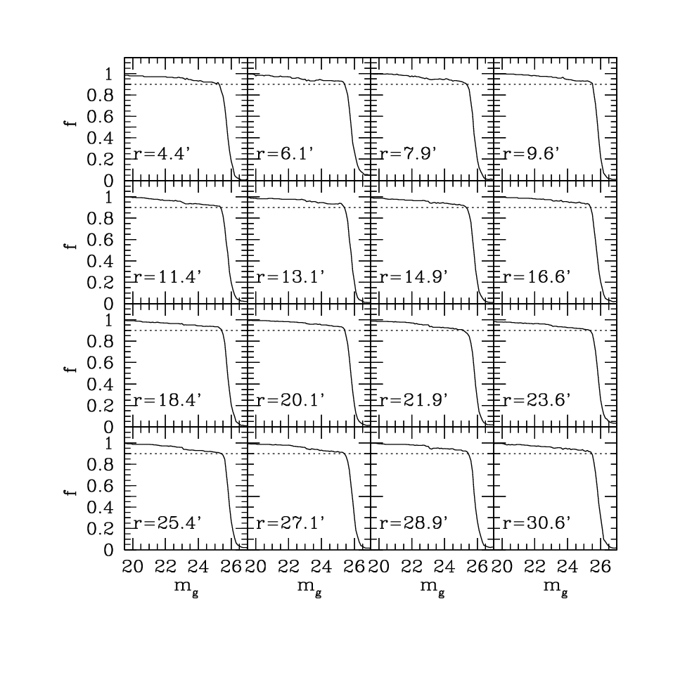
The completeness function of the -band images was determined by adding artificial stars to the original images and then reprocessing them as described in Section 3. The ratio between the number of artificial stars added, and the number of stars recovered provides the estimate of the completeness. We added stars using a grid pattern, with increments in x and y. Since the field is dominated by the light from NGC 3115, the correction for magnitude completeness depends on the angular distance from the galaxy center (Cantiello et al., 2007, e.g.). The radial dependent completeness function is shown in Figure 15. To correct the luminosity functions the number of objects at given magnitude is multiplied by using the proper function at each galactocentric distance.
A.2 Edge detection filter

In Figure 16 we analyze the behavior of the edge-detection function on a composite function similar to the one expected for the sources in the field of NGC 3115. The function inspected is the sum of a gaussian GCLF (Harris, 2001) and a power law for background galaxies (Tyson, 1988; Bernstein et al., 2002), times a completeness smoothed step function (green, blue and red line, respectively). The edge-detection function, in a first approximation, is a derivative function and shows an inflection point at the GCLF turnover magnitude (Figure 16, middle panel). A second run of the edge function - Edge2, roughly a second derivative - reaches a local extrema at the TOM. Thus, in first approximation, the turnover of the GCLF can be found in correspondence of an inflection and a local extrema in the Edge and Edge2 functions, respectively.
Appendix B Some details on Ishape
Ishape uses a PSF subsampled by a factor 10 relative to the resolution of the science image. To model the PSF we used the DAOPHOT package within IRAF and, to reduce the chance of contaminating the PSF modeling with GCs in the galaxy, we included in the list of PSF candidates unsaturated sources with , and mag. To account for PSF variations across the image, we set DAOPHOT VARORDER=2, which means that the PSF is quadratically variable over the image. Then, the frame was divided in a grid of equal subframes, and the model PSF for Ishape evaluated in the center of each subframe.
Within Ishape, we adopted the “KING30” profile, i.e. the King (1962) model with concentration parameter , which is typical for marginally resolved GCs and UCDs (Larsen & Richtler, 2000; Blakeslee & Barber DeGraaff, 2008).
| Parameter | Value | Explanation |
|---|---|---|
| PSF | Moffat25 | Input PSF from DAOPHOT |
| FITRAD | 12 | Fitting radius |
| CENTERRAD | 3 | Maximum centering radius |
| CLEANRAD | 3 | Cleaning radius |
| CTRESH | 2 | Threshold for cleaning |
| MAXCITER | 5 | Maximum number of iterations |
| CENTERMETHOD | MAX | Centering method |
| SHAPE | KING30 | Shape used for profile fitting |
| FWHMMAX | 20.0 | Maximum FWHM |
| ITMAX | 200 | Maximum number of iterations |
| ELLIPTICAL | YES | Use elliptical model |
| EPADU | 11.5 | /ADU conversion factor |
| RON | 7.0 | CCD read-out noise |
| CALCERR | YES | Calculate errors |
In order to determine the best parameters for Ishape we performed a reference run and various tests changing the input parameters. Table 5 gives the main parameters for the reference run (g1 label). The other tests are obtained as follows: test#1 we adopted the DAOPHOT Penny1 PSF instead of the Moffat25 (label g2); for test#2 and #3 (labels g3 and g4) we used Ishape fitting radius 9 pixels and 15 pixels, respectively; test#4: the maximum FWHM is set to 40 pixels (label g5); test#5: does not fit an elliptical model, circular symmetry is used instead (label g6). In all cases, except for the test #6, the FWHM is transformed to circularized effective radius , where and are the full width, and the axis ratio fitted by Ishape1111 11 This equation, suggested in the Ishape handbook, provides results nearly identical to the one used by other authors (Blakeslee & Barber DeGraaff, 2008, e.g.).. For the test #6 we used . Figure 17 shows the results of the Ishape tests. The data in the figure show that, in general, there can be even a factor 10 difference between estimates with different Ishape input parameters. Nevertheless, for the reference sample (see Section 5), the effect of changing fitting parameters implies a median change on of . We also inspected the correlation between the radius and magnitude of the sources, and did not find any.
Figure 18 shows the VEGAS-SSS to ACS comparison for the various tests. The data in the figure show that the results with the reference g1 run are broadly consistent with the other tests. We note that, in choosing the best parameters for Ishape, we also took into account the number of sources successfully analyzed by the tool. For the g1 test the input catalog contained sources, and the spatial parameters were obtained for . Such number can decrease significantly for other choices of the input parameters – most notably in the test g4.


Appendix C On some UCDs in Jennings et al. (2014)
As discussed in Section 5, and shown in Figure 9, we found a good match with ACS photometry. Figure 19 shows that the photometric matching is not as good for some of the UCD candidates in Jennings et al. catalog (empty circles). The mismatch cannot be simply explained by the different aperture correction, since, as described in Jennings et al. (2014, Section 2.4.1), the largest aperture correction is 0.94 mag, and we find differences up to mag.
To understand what the issue is, we downloaded one of the ACS pointings of NGC 3115 (choosing the one maximizing the number of UCDs over the frame), and independently derived the photometry of SSSs candidates using the same methods and tools described in Section §3. Figure 20 shows the comparison VEGAS-SSS magnitudes (), with our photometry from ACS images (), and with Jennings et al. (2014) (). From the latter test, we find that, while the agreement for GC photometry is still acceptable, the large difference between ACS and VEGAS-SSS UCD data disappears (right panel in the figure). The large scatter for the GCs is mainly due to the use of only one of the ACS pointings available.
As a further check, for the UCDs in common with the ACS pointing analyzed, we also compared magnitudes and effective radii for VEGAS-SSS, using a different photometric tool, 2Dphot (La Barbera et al., 2008, test kindly carried out by F. La Barbera), and found a good matching between the results of our standard procedures and the ones from 2Dphot (Figure 21, upper right and lower panels).
A visual inspection of some UCD candidates from Jennings et al. (2014) reveals possible problems with the identification of sources. The cases shown, infact, reveal that UCD10 (the object with the largest difference in the Figures 19-20) and UCD20 from the Jennings et al. list, are actually a spiral galaxy and an object immersed in system with clear merging features (tidal streams?).


