A Clearer Picture of Blind Deconvolution
Abstract
Blind deconvolution is the problem of recovering a sharp image and a blur kernel from a noisy blurry image. Recently, there has been a significant effort on understanding the basic mechanisms to solve blind deconvolution. While this effort resulted in the deployment of effective algorithms, the theoretical findings generated contrasting views on why these approaches worked. On the one hand, one could observe experimentally that alternating energy minimization algorithms converge to the desired solution. On the other hand, it has been shown that such alternating minimization algorithms should fail to converge and one should instead use a so-called Variational Bayes approach. To clarify this conundrum, recent work showed that a good image and blur prior is instead what makes a blind deconvolution algorithm work. Unfortunately, this analysis did not apply to algorithms based on total variation regularization. In this manuscript, we provide both analysis and experiments to get a clearer picture of blind deconvolution. Our analysis reveals the very reason why an algorithm based on total variation works. We also introduce an implementation of this algorithm and show that, in spite of its extreme simplicity, it is very robust and achieves a performance comparable to the state of the art.
Index Terms:
Deblurring, blind deconvolution, total variation.Blind deconvolution is the problem of recovering a signal and a degradation kernel from their noisy convolution. This problem is found in diverse fields such as astronomical imaging, medical imaging, (audio) signal processing, and image processing. More recently, blind deconvolution has received renewed attention due to the emerging need for removing motion blur in images captured by mobile phones [1]. Yet, despite over three decades of research in the field (see [2] and references therein), the design and analysis of a principled, stable and robust algorithm that can handle real images remains a challenge. However, present-day progress has shown that recent models for sharp images and blur kernels can yield remarkable results [1, 3, 4, 5, 6].
Many of these recent approaches are evolutions of the variational formulation [7]. A common element in these methods is the explicit use of priors for both blur and sharp image to encourage smoothness in the solution. Among these recent methods, total variation emerged as one of the most popular priors [8, 9]. Such popularity is probably due to its ability to encourage gradient sparsity, a property that can describe many signals of interest well [10].
However, recent work by Levin et al. [11] has shown that the joint optimization of both image and blur kernel can have the no-blur solution as its global minimum. That is to say, blind deconvolution algorithms that use a total variation prior either are local minimizers and, hence, require a lucky initial guess, or they cannot depart too much from the no-blur solution. Nonetheless, algorithms based on the joint optimization of blur and sharp image show good convergence behavior even when initialized with the no-blur solution [8, 3].
This incongruence called for an in-depth analysis of total variation blind deconvolution (TVBD). As we show in the next sections, the answer is not as straightforward as one might have hoped. Firstly, we confirm both experimentally and analytically the analysis of Levin et al. [11]. Secondly, we also find that the algorithm of Chan and Wong [8] converges to the desired solution, even when starting at the no-blur solution. The answer to this puzzle lies in the specific implementation of [8], as it does not minimize the originally-defined energy. This algorithm, as commonly done in many other algorithms, separates some constraints from the gradient descent step and then applies them sequentially. When the cost functional is convex this alteration may not have a major impact. However, in blind deconvolution, where the cost functional is not convex, this completely changes the convergence behavior. Indeed, we show that if one imposed all the constraints simultaneously then the algorithm would never leave the no-blur solution independently of the regularization amount.
To further demonstrate our findings, we implement a TVBD algorithm without the use of all recent improvements, such as filtering [3, 4, 11], blur kernel prior [8, 9] or edge enhancement [4, 5], and show that applying sequentially the constraints on the blur kernel is sufficient to avoid the no-blur solution. We also show that the use of a filtered version of the original signal may be undesirable and that the use of exact boundary conditions can improve the results. Finally, we apply the algorithm on currently available datasets, compare it to the state of the art methods and show that, notwithstanding its simplicity, it achieves a comparable performance to the top performers.
I Blur Model and Priors
Suppose that a blurry image can be modeled by
| (1) |
where is a blur kernel, a sharp image, noise and denotes convolution between and . Given only the blurry image, one might want to recover both the sharp image and the blur kernel. This task is called blind deconvolution. A classic approach to this problem is to maximize the posterior distribution (MAPu,k)
| (2) |
where models the noise affecting the blurry image, models the distribution of typical sharp images, and is the prior knowledge about the blur function. Typical choices for are the Gaussian distribution [1, 6] or the exponential distribution [5]. In the following discussion we will assume that is modeled by a Gaussian distribution.
Through some standard transformations and assumptions, problem (2) can be written also as a regularized minimization
| (3) |
where the first term corresponds to , the functionals and are the smoothness priors for and (for example, Tikhonov regularizers [12] on the gradients), and and two nonnegative parameters that weigh their contribution. Furthermore, additional constraints on , such as positivity of its entries and integration to , can be included. For any and the cost functional will not have as global solution neither the true solution nor the no-blur solution , where denotes the Dirac delta. Indeed, eq. (3) will find an optimal tradeoff between the data fitting term and the regularization term. Nonetheless, one important aspect that we will discuss later on is that both the true solution and the no-blur solution make the data fitting term in eq. (3) equal to zero. Hence, we can compare their cost in the functional simply by evaluating the regularization terms. Notice also that the minimization objective in eq. (3) is non-convex, and, as shown in Fig. 4, has several local minima.
(a)
(b)
II Prior work
To solve problem (3) one has to carefully choose the functions and . A common choice is the norm of and or of some filtered versions of and .
has been defined as the norm of [7, 5, 4], a sparsity-inducing norm () [1, 3] or a constant [6]. Nonetheless, its contribution to the estimation of the desired solution is so far marginal. In fact, some methods successfully solve problem (3) by setting . Yet, it has been shown that its use may help avoid undesired local minima [13].
The regularization term for the sharp image instead has a stronger impact on the performance of the algorithm, since it helps choose a sharp image over a blurry one. You and Kaveh [7] have proposed to use the norm of the derivatives of . Unfortunately, this norm is not able to model the sparse nature of common image gradients and results in sharp images that are either oversmoothed or have ringing artifacts. Yet, the norm has the desirable property of being efficient to minimize. Cho and Lee [4] and Xu and Jia [5] have reduced the generation of artifacts while still retaining its computational efficiency by using heuristics to select sharp edges.
An alternative to the norm is the use of total variation (TV) [8, 9, 14, 15]. TV regularization was firstly introduced for image denoising in the seminal work of Rudin, Osher and Fatemi [16], and since then it has been applied successfully in many image processing applications. Total variation is typically defined via two different formulations. Its anisotropic version is the sum of the norms of the components of the gradient of , while its isotropic version is the norm of the gradient of .
You and Kaveh [9] and Chan and Wong [8] have proposed the use of TV regularization in blind deconvolution on both and . They also consider the following additional convex constraints to enhance the convergence of their algorithms
| (4) |
where with we denote either 1D or 2D coordinates. He et al. [15] have incorporated the above constraints in a variational model, claiming that this enhances the stability of the algorithm. A different approach is a strategy proposed by Wang et al. [17] that seeks for the desired local minimum by using downsampled reconstructed images as priors during the optimization in a multi-scale framework.
TV regularization has been widely popularized because it models natural image gradients well [10]. Wipf and Zhang [18] have recently argued that should not merely try to model statistics of sharp images, but, rather, it should have a strong discriminative power in separating sharp from blurry images. This is ideally achieved by using the pseudo-norm on the image gradients. Unfortunately its exact minimization requires solving an NP-hard problem. To make the problem tractable some methods have proposed to use approximations of the norm [19, 20]. Yet, the proposed approximations are non-convex functions that require careful minimization strategies to avoid local minima.
The algorithms presented so far are all successful implementation of the MAPu,k formulation in (2), nonetheless Levin et al. [11] have shown that using an norm of the image gradients with any and a uniform distribution for the blur, the MAPu,k approach favors the no-blur solution , for images blurred with a large enough blur. They also argue that the success of existing MAPu,k methods is due to various heuristics or reweighing strategies employed during the optimization of (3).
Because of the above concerns, Levin et al. [11] look at a different strategy that marginalizes over all possible sharp images . They solve the following MAPk problem
| (5) |
where the sharp image is estimated by solving a convex problem and where is given from the previous step. They have shown that, for sufficiently large images, the MAPk approach converges to the true solution. Since the right hand side of problem (5) is difficult to compute, it is common to use a Variational Bayesian approach (VB) where one aims at finding an approximation of the probability [21, 1, 22, 18, 6].
In recent work, Wipf and Zhang [18] have shed new light on the MAPu,k vs MAPk dispute. They have shown that the VB formulation commonly used to solve the MAPk is equivalent to a non-conventional MAPu,k approach, and that priors with are able to favor sharp images. They also argue that a VB approach is still preferable because it is more able to avoid local minima compared to a classical MAPu,k approach.
The work of Wipf and Zhang [18] has focused on priors with and given novel insights on the mechanism that make them work. Our work complements the results of Wipf and Zhang [18] and focuses on the total variation () prior. We confirm the theoretical results of Levin et al. [11] and show that an apparently harmless delayed normalization induces a scaling of the signal that ultimately results in the success of total variation based algorithms. This shows that filtered version of the images [3, 4, 11], blur kernel prior [8, 9], edge enhancement [4, 5] or any other additional strategy are not necessary for solving blind deconvolution.
III Problem Formulation
By combining problem (3) with the constraints in eq. (4) and by setting , we study the following minimization
| (6) |
where or , with the gradient of and , and corresponds to the norm in eq. (4). To keep the analysis simple we have stripped the formulation of all unnecessary improvements such as using a basis of filters in [3, 4, 11], or performing some selection of regions by reweighing the data fitting term [5], or enhancing the edges of the blurry image [5, 4]. Compared to previous methods, we also do not use any regularization on the blur kernel ().
The formulation in eq. (6) involves the minimization of a constrained non-convex optimization problem. Also, notice that if is a solution, then are solutions as well for any . If the additional constraints on were not used, then the ambiguities would also include for non zero .
(a)
(b)
(c)
III-A Convolution Models and Notation
The convolution operator in the minimization (6) usually requires some assumptions on the boundaries of the image. We instead propose a new formulation that does not make any boundary assumptions.
Let and be matrices with the same support , and a matrix with support . Typically the discrete convolution of and is defined by
| (7) |
for , , where some assumptions are made on the values outside the support of (Fig. 1a). Commonly used assumptions in the literature are: symmetric, where the boundary of the image is mirrored to fill the additional frame around the image; periodic, where the image is padded with a periodic repetition of the boundary; replicate, where the borders continue with a constant value. The periodic assumption is particularly convenient because it allows the use of the circular convolution theorem and the Discrete Fourier Transform (DFT) to achieve a fast performance. Because real images are rarely periodic, Liu and Jia [23] have proposed to extend the size of the blurry image to make it periodic. Nonetheless, each of the above choices is an approximation of the real physical phenomenon and therefore it introduces an error in the reconstruction of the sharp image.
In this paper we propose to use a different approach, where the blurry image has support . In this case we define a new convolution operator, denoted by , as
| (8) |
for , and where (Fig. 1b). Notice that in general. Also, is not defined if the support of is too large ( and ).
In the following we will choose to be the isotropic total variation . By incorporating the above considerations in a discrete setting, the problem in (6) can be written as
| (9) |
where , and 11 1 Notice that represents the support of and the support of ..
Since in (9) the domain of the sharp image is larger than the domain of the blurry image , solving (9) requires the estimation of more variables than measurements. This problem is tackled by the total variation term that imposes a weak smoothness constraint beyond the boundary of , instead of the hard assumptions needed when using eq. (7). We will show that using this formulation gives better results compared to the typical approach that uses eq. (7).
IV Analysis of Total Variation Blind Deconvolution
Recent analysis has highlighted important limitations of the total variation prior regarding the blind deconvolution problem. Still, as mentioned in the Prior Work section many algorithms successfully employ total variation for solving this problem. In this section we confirm the limitations of total variation highlighted in previous work [11], and show how a small detail in the minimization strategy commonly used by many algorithms allows them to avoid local minima and estimate the correct blur.
In Section IV-A we show that an norm with can not favor the reconstruction of a sharp image over a blurry one. Therefore, when used in problem (9) it does not yield the desired solution.
To understand why many algorithms still succeed, in Section IV-B we study the Alternating Minimization (AM) algorithm, which computes a local optimum of problem (9). To facilitate its analysis, it is desirable to have closed-form solutions at each step. However, in 2D there are no known closed-form solutions for any of the steps. Hence, we consider the 1D formulation and initialize the algorithm with the no-blur solution, which makes the first iteration equivalent to a total variation denoising problem (as opposed to a deconvolution problem). It is then possible to estimate a closed-form solution in the 1D case by using the taut string algorithm of Davies and Kovacs [25]. Moreover, in Section IV-C we work with a step function and a pixel blur, and we show how it is possible to estimate a sharp, but scaled, signal from the first step of the AM algorithm (which we call TV-signal in Fig. 2 (a)). In Section IV-D we also show that it is possible to have a similar behavior by using a filtered version of the signals. However, in Section IV-E we show how the use of the original signals may still be preferable.
By using the solution of the 1D total variation denoising problem, in Section IV-F we show that a rigorous application of the AM algorithm gives the undesired no-blur solution in its second step. In fact, as shown in Fig. 2 (b), any blur different from the Dirac delta function would increase the difference between the input blurry signal (red plot) and the blurred TV signal (black plot). In Section IV-G we point out that typical blind deconvolution algorithms do not solve the AM algorithm but a variant, which we call Projected Alternating Minimization (PAM) algorithm, where the constraints on the blur kernel are imposed separately in a delayed step. In Section IV-H we show how this detail makes the PAM algorithm estimate in its second stage the true blur kernel. The delayed enforcement of the constraints can be seen as equivalent to a scaling of the TV denoised signal (see Fig. 2 (c)). Finally, in Section IV-I we highlight the role of the regularization parameter and further stress the importance of the scaling principle to make the PAM algorithm succeed.
IV-A Analysis of Relevant Local Minima
In this section we study the norm of the image derivatives as image prior, with a particular emphasis to the case of . In a recent work Levin et al. [6] have shown that eq. (6) favors the no-blur solution , when , for any and either the true blur has a large support or . In the following theorem we show that the above result is also true for any kind of blur kernels and for an image prior with .
Theorem IV.1
Let , with , be the noise-free input blurry image () and the sharp image. Then,
| (10) |
Proof:
Because is noise-free, ; since the convolution and the gradient are linear operators, we have
| (11) |
By applying Young’s inequality [26] (see Theorem 3.9.4, pages 205-206) we have
| (12) |
since . ∎Since the first term (the data fitting term) in problem (6) is zero for both the no-blur solution and the true solution , Theorem IV.1 states that the no-blur solution has always a smaller, or at most equivalent, cost than the true solution. Notice that Theorem IV.1 is also valid for any for any . Thus, it includes as special cases the Gaussian prior , when , , and the anisotropic total variation prior , when , .
IV-B The Alternating Minimization (AM) Algorithm
To better understand the behavior of a total variation based blind deconvolution algorithm we consider an alternating minimization algorithm that minimizes (9). The solution is found by alternating between the estimation of the sharp image given the kernel and the estimation of the kernel given the sharp image. This approach, which we call the AM algorithm, requires solving an unconstrained convex problem in
| (13) |
and a constrained convex problem in
| (14) |
A convergence analysis of the AM algorithm is still challenging, but when the algorithm is initialized at the no-blur solution, the first step of the AM algorithm requires solving a denoising problem
| (15) |
The total variation denoising algorithm (15) has been widely studied in the literature, and its analysis can give key insights on the behavior of the AM algorithm. In the next section we study this problem and present an important building block for the other results presented in the paper.
IV-C Analysis of 1D Total Variation Denoising
In this section we look at the solution of a 1D total variation denoising problem because analysis of problem (9) in the literature is still fairly limited and a closed-form solution even for a restricted family of 2D signals is not available. Still, analysis in 1D can provide practical insights.
A total variation denoising problem can be written in 1D as
| (16) |
where and . For a successful convergence of the AM algorithm it is desirable to have a solution equal or close to the true sharp signal . By exploiting recent work of Condat [27], Strong and Chan [28] and the taut string algorithm of Davies and Kovacs [25], for a simple class of signals, in the following proposition we give the analytical expression for that gives a sharp, but scaled, version of as the solution of the denoising problem (16).
Proposition IV.2
Let be a 1D step function of the following form
| (17) |
for some and , and be a 3-element blur kernel where , and , and . Then, is the convolution of with
| (18) |
The solution to the problem (16) is
| (19) |
when , is
| (20) |
when , and is
| (21) |
when . Analytical expressions for , , , , , , , , are defined in Table I. If or then a that gives the solution (19), (20) or (21) does not exist.
Proof:
See Section A-A. ∎Proposition IV.2 shows that for a wide range of signals it is possible to obtain a sharp signal by solving problem (16). Notice, however, that total variation regularization locally scales the input signal (see also illustration in Fig 2 (a)). We will show in the next sections that this apparently insignificant scaling has a fundamental role in the convergence of the AM algorithm.
IV-D Filtered Image Model
A common practice in many MAPk methods that use a Variational Bayesian approach is to solve problem (9) using the gradients of and instead of the original signals [1, 18, 6]. In this section we briefly consider this case for the AM algorithm. In this case the 1D denoising problem of (16) becomes
| (22) |
where and . Problem (22) can be easily solved in closed form by soft-thresholding, therefore for a simple class of signals as in Proposition IV.2 we can seek for values of such that the solution is the derivative of a sharp signal, i.e., a Dirac delta.
Theorem IV.3
Proof:
See Section A-B. ∎Theorem IV.3 gives conditions on such that the TV denoising of filtered signals gives a scaled version of the true sharp signal. This result is similar to the one given by Proposition IV.2 for the classical TV denoising algorithm, nonetheless there are still important differences that we highlight in the next section.
IV-E Existence of Sharp Signal Solutions
Both Theorem IV.3 and Proposition IV.2 give conditions such that it is possible to estimate a sharp signal from a blurry one by solving a denoising problem. An important question is to ask under what conditions a sharp signal can not be estimated from a blurry one. We will consider the space of all possible 3-element blurs parametrized in and and call degenerate region the configurations for which a sharp signal can not be estimated. Notice that the degenerate region corresponds to signals where it is only possible to remove one of the two steps of the blurry signal, or where the minimum required to get a sharp signal is equal to the one that makes the whole signal constant.
For the classical TV denoising algorithm from Theorem IV.3 we have that if the true blur lies on two lines, parametrized on and , then it is not possible to estimate a sharp signal (see Fig. 3 (a) and (b)). Because of the parametrization on and , different signals have different degenerate regions. We can generalize the discussion to a general piecewise constant signal by dividing it in many step signals. Thus, the denoising problem of a piecewise signal is equivalent to many denoising problems of different step signals with careful treatment at the boundaries. If each signal has different degenerate regions, it is likely that for each blur configuration the majority of the signal will not be in a degenerate case.
For the TV denoising of the filtered signal, the degenerate region is denoted by three segments (see Fig. 3 (c)). Since it is the same for any possible signal, it would not be changed by considering a general piecewise signal as in the case of problem (9). Thus, in this case it is not possible to deblur images blurred with blurs that lie in the degenerate case.
The above discussion is intentionally informal, as providing a formal proof would require too much space. Still, it suggests that there may be aspects, previously not considered in the literature, that support the use of the original signal in problem (9) in lieu of their filtered versions.

a)

b)

c)
IV-F Analysis of the AM Algorithm
The study of the total variation denoising algorithm is important because it represents the first step of the AM algorithm, when the blur is initialized with a Dirac delta. In the next theorem we show how the exact AM algorithm can not leave the no-blur solution when is defined as in (18) and the first step of the AM algorithm gives as a solution a sharp signal.
Theorem IV.4
Let , and be the same as in Proposition IV.2. Then, for a , or the AM algorithm converges to the solution .
Proof:
See Section A-C. ∎
The result in Theorem IV.4 confirms what it has been concluded by Theorem IV.1. In the next section we show a variant of the AM algorithm, which is commonly used in many other blind deconvolution papers, that behave in a completely different way than the AM algorithm for the same class of signals of Proposition IV.2.
IV-G The Projected Alternating Minimization (PAM) Algorithm
Many methods in the literature minimize problem (9) by using a variant of the AM algorithm. This variant consists in alternating between minimizing the unconstrained convex problem (13) in as in the AM algorithm, and an unconstrained convex problem in
| (26) |
followed by two sequential projections where one applies the constraints on the blur , i.e.,
| (27) |
We call this iterative procedure the PAM algorithm. The choice of imposing the constraints sequentially rather than during the gradient descent on seems a rather innocent and acceptable approximation of the correct procedure (AM). However, this is not the case and we will see that with this arrangement one can achieve the desired solution.
IV-H Analysis of the PAM Algorithm
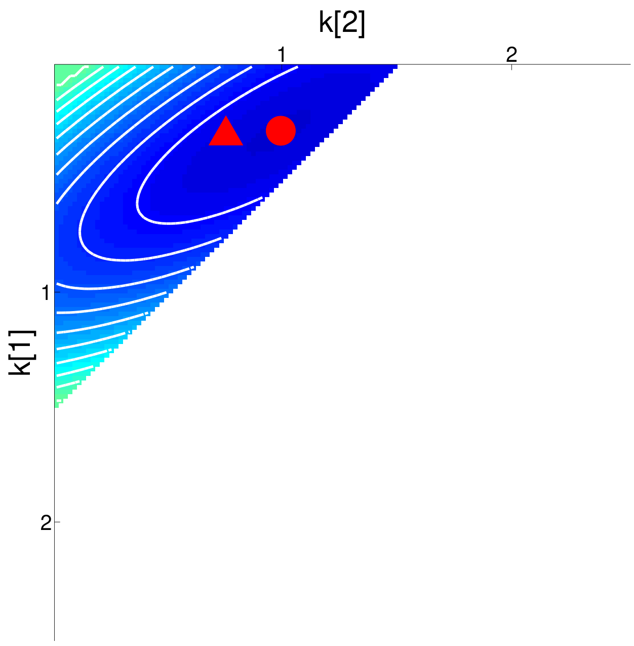
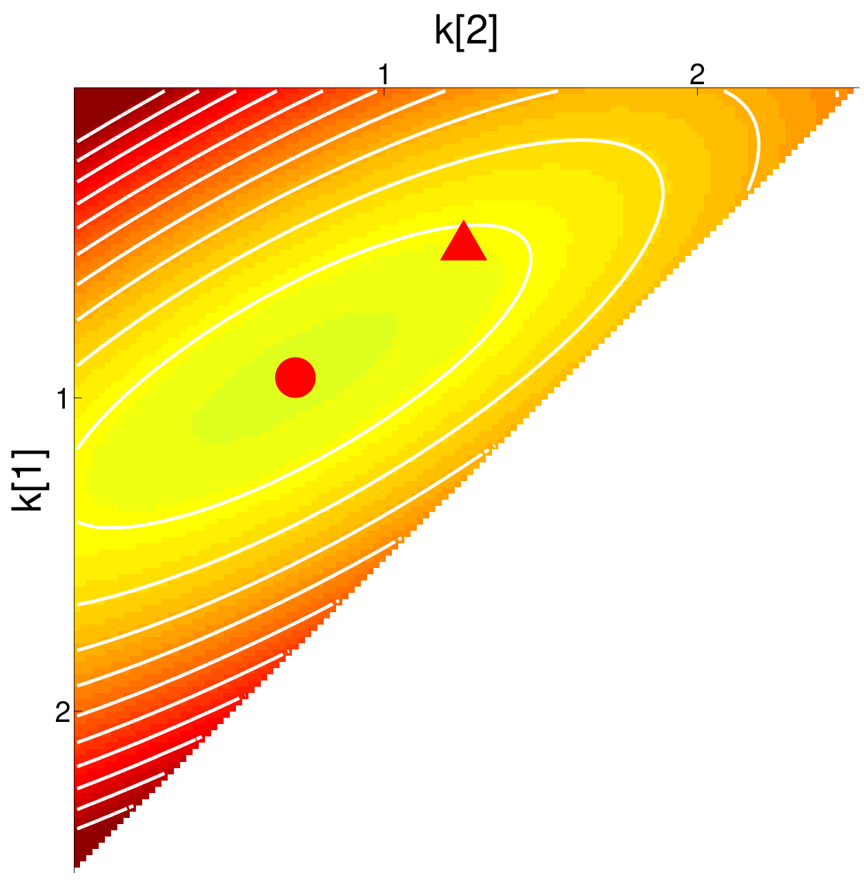
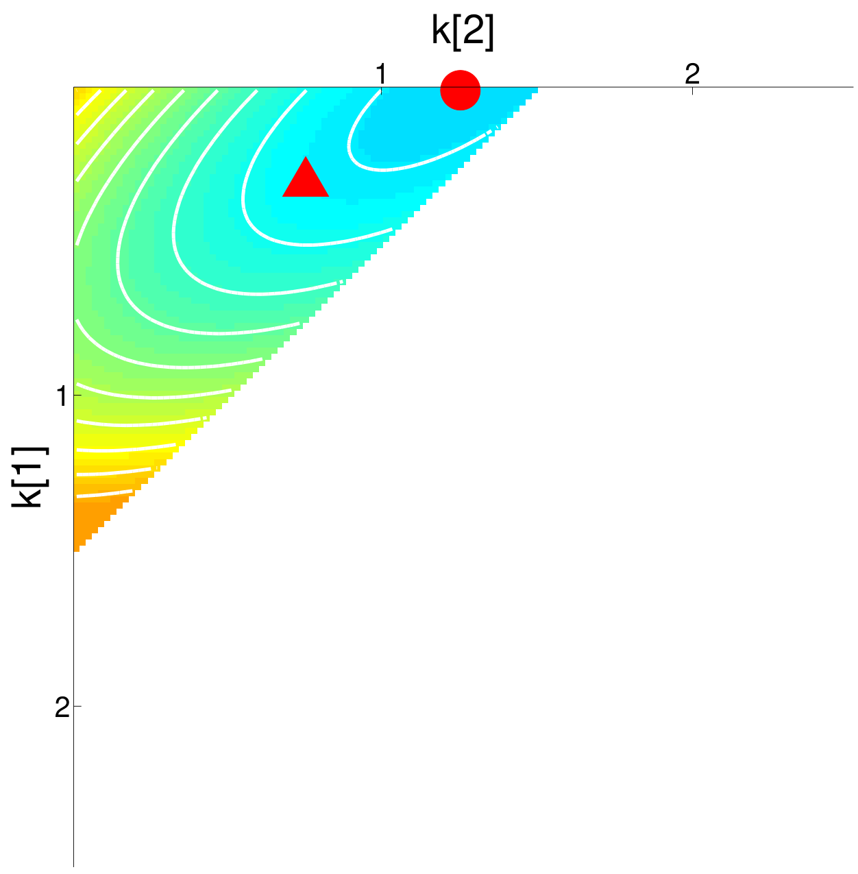
Our first claim is that this procedure does not minimize the original problem (6). To support this claim we start by showing some experimental evidence in Fig. 4. In this test we work on a 1D version of the problem. We blur a hat function with one blur of size pixels, and we show the minimum of eq. (9) for all possible feasible blurs. Since the blur has only nonnegative components and must add up to , we only have free parameters bound between and . Thus, we can produce a 2D plot of the minimum of the energy with respect to as a function of these two parameters. The blue color denotes a small cost, while the red color denotes a large cost. The figures reveal three local minima at the corners, due to the different shifted versions of the no-blur solution, and the local minimum at the true solution () marked with a yellow triangle. We also show with white dots the path followed by estimated via the PAM algorithm by starting from one of the no-blur solutions (upper-right corner). Clearly one can see that the PAM algorithm does not follow a minimizing path in the space of solutions of problem (9), and therefore does not minimize the same energy.
Furthermore, we show how the PAM algorithm succeeds in estimating the true blur in two steps whereas the AM algorithm estimates a Dirac delta.
Theorem IV.5
Let , and be the same as in Proposition IV.2. Let also constraint to be a zero-mean signal.
Then, if there exists a , or the PAM algorithm estimates the true blur (or a shifted version of it) in two steps, when starting from the no-blur solution pair .
Proof:
See Section A-D. ∎




IV-I Discussion
Theorems (IV.5) and (IV.4) show that with 1D zero-mean step signals and no-blur initialization, for some values of PAM converges to the correct blur (and only in steps) while AM does not. We used a step signal to keep the discussion simple and because it is fundamental to illustrate the behavior of both algorithms at edges in a 2D image. However, as already mentioned in sec. IV-E, extensions of the above results to blurs with a larger support and beyond step functions are possible by dividing the signal in many step functions and by a careful treatment of the boundaries.
In Fig. 5 we illustrate two further aspects of Theorem IV.5 (it is recommended that images are viewed in color): 1) the advantage of a non unitary normalization of during the optimization step (which is a key feature of PAM) and 2) the need for a sufficiently large regularization parameter . In the top row images we set . Then, we show the cost , with , for all possible 1D blurs with a -pixel support under the constraints respectively. This is the cost that PAM minimizes at the second step when initialized with . Because has three components and we fix its normalization, we can illustrate the cost as a 2D function of and as in Fig. 4. However, as the normalization of grows, the triangular domain of and increases as well. Since the optimization of the blur is unconstrained, the optimal solution will be searched both within the domain and across normalization factors. Thanks to the color coding scheme, one can immediately see that the case of achieves the global minimum, and hence the solution is the Dirac delta. However, as we set in the second row or in the bottom row, we can see a shift of the optimal value for non unitary blur normalization values and also for a shift of the global minimum to the desired solution (bottom-right plot).
V Implementation
In Algorithm 1 we show the pseudo-code of our adaptation of TVBD. At each iteration we perform just one gradient descent step on and on as proposed by Chan and Wong [8] because we experimentally noticed that this speeds up the convergence of the algorithm. The gradient descent results in the following update for the sharp image at the -th iteration
| (28) |
for some step where and denotes the discrete convolution operator where the result is the full convolution region, i.e., if , with , , then we have with zero padding as boundary condition. The iteration on the blur kernel is instead given by
| (29) |
From Theorem (IV.5) we know that a big value for the parameter helps avoiding the no-blur solution, but in practice it also makes the estimated sharp image too “cartooned”. We found that iteratively reducing the value of as specified in Algorithm 1 helps getting closer to the true solution.
In the following paragraphs we highlight some other important features of Algorithm 1.
Pyramid scheme.
While all the theory holds at the original input image size, to speed up the algorithm we also make use of a pyramid scheme, where we scale down the blurry image and the blur size until the latter is pixels. We then launch our deblurring algorithm from the lowest scale, then upsample the results and use them as initialization for the following scale. This procedure provides a significant speed up of the algorithm. On the smallest scale, we initialize our optimization from a uniform blur.
Color images.
For the blur estimation many methods first convert color images to grayscale. In contrast with this common practice, we extended our algorithm to work directly with color images. Recently, many papers have proposed algorithms for color denoising using TV regularization [29, 30, 31]. In our implementation we use the method of Blomgren and Chan [31], and all the results on color images that we show in this papers are obtained by solving the blind-deconvolution problem on the original color space.
VI Experiments
We evaluated the performance of our algorithm on several images and compared with state-of-the-art algorithms. We provide our unoptimized Matlab implementation on our website22 2 http://www.cvg.unibe.ch/dperrone/tvdb/. Our blind deconvolution implementation processes images of pixels with blurs of about pixels in around 2-5 minutes, while our non-blind deconvolution algorithm takes about seconds.
In our experiments we used the dataset from [11] in the same manner illustrated by the authors. For the whole test we used . We used the non-blind deconvolution algorithm from [32] with and for each method we compute the cumulative histogram of the deconvolution error ratio across test examples, where the -th bin counts the percentage of images for which the error ratio is smaller than . The deconvolution error ratio, as defined in [11], measures the ratio between the SSD deconvolution error with the estimated and correct kernels. In Fig. 8 we show the cumulative histogram of the error ratio for Algorithm 1, the algorithm of Levin et al. [32], the algorithm of Fergus et al. [1], the algorithm of Babacan et al. [22], the algorithm of Wipf and Zhang [18] and the one of Cho and Lee [4]. Algorithm 1 performs on par with the one from Levin et al. [32], with a slightly higher number of restored images with small error ratio.
In Fig. 9 we show a comparison between our method and the one proposed by Xu and Jia [5]. Their algorithm is able to restore sharp images even when the blur size is large by using an edge selection scheme that selects only large edges. This behavior is automatically minimicked by Algorithm 1 thanks to the TV prior. Also, in the presence of noise, Algorithm 1 performs visually on a par with the state-of-the-art algorithms as shown in Fig. 10.
Recently Köhler et al. [33] introduced a dataset of images blurred by camera shake blur. Even if this kind of artifact produces space-varying blur, many algorithms that assume shift-invariant blur perform well on many images of the dataset. In Fig. 11 we show an example from the dataset of [33] where our algorithm is as robust to camera shake blur as other shift-invariant algorithms.
For testing purposes we also adapted our algorithm to support different boundary conditions by substituting the convolution operator described in (8) with the one in (7).
In Fig. 8 we show a comparison on the dataset of [11] between our original approach and the adaptations with different boundary conditions. For each boundary condition we evaluated the ratios between the SSD deconvolution errors of the estimated and correct kernels. The implementations with the different boundary conditions perform worse than our free-boundary implementation, even if pre-processing the blurry image with the method of Liu and Jia [23] considerably improves the performance of the periodic boundary condition.
Recent algorithms estimate the blur by using filtered versions of and in the data fitting term (typically the gradients or the Laplacian) . This choice might improve the estimation of the blur because it reduces the error at the boundary when using any of the previous approximations, but it might result also in a larger sensitivity to noise. In Fig. 8 we show how with the use of the filtered images for the blur estimation the performance of the periodic and replicate boundary conditions improves, while the others get slightly worse. Notice that our implementation still achieves better results than other boundary assumptions.

Blurry Input.

Restored image and blur with Xu and Jia [5].

Restored image and blur with Algorithm 1.

Blurry Input.

Cho and Lee [4].

Levin et al. [6].

Goldstein and Fattal [34].

Zhong et al. [35].

Algorithm 1.

Blurry Input.

Restored image with Cho and Lee [4].

Restored image with Fergus et al. [1].

Restored image with Krishnan et al. [20].

Restored image with Xu and Jia [5].

Restored image with Whyte et al. [36].

Restored image with Shan et al. [3].

Restored image with Xu et al. [19].

Restored image with our algorithm.
VII Conclusions
In this paper we shed light on approaches to solve blind deconvolution. First, we confirmed that the problem formulation of total variation blind deconvolution as a maximum a priori in both sharp image and blur () is prone to local minima and, more importantly, does not favor the correct solution. Second, we also confirmed that the original implementation [8] of total variation blind deconvolution (PAM) can successfully achieve the desired solution. This discordance was clarified by dissecting PAM in its simplest steps. The analysis revealed that such algorithm does not minimize the original formulation. This analysis applies to a large number of methods solving as they might exploit the properties of PAM; moreover, it shows that there might be principled solutions to . We believe that by further studying the behavior of the PAM algorithm one could arrive at novel useful formulations for blind deconvolution. Finally, we have showed that the PAM algorithm is neither worse nor better than the state of the art algorithms despite its simplicity.
Appendix A
In the appendix we show the proofs of the propositions and of the theorems presented in the paper.
A-A Proof of Proposition IV.2
Proof:
Solving problem (16) is equivalent to solving the following problem
| (30) | |||
where for , and . In the following, unless specified, we will always refer to problem (30).
The solution of problem (30) can also be written as , , where is found by solving the taut string problem (e.g., see Davies and Kovac [25])
| (31) | ||||
| s.t. | ||||
where with .
Given the explicit form of in eq. (18) we obtain that
| (32) |
Notice that has three discontinuities at , and . Let consider solving the taut string problem by enforcing in turn only the constraint , and .
For the first case the cost of the taut string problem is minimum for the shortest path through a point at . We can decompose such path into the concatenation of the shortest path from to and the shortest path from to . Given that each of these paths are only constrained at the end points, a direct solution will give a line segment between the end points, i.e.,
| (33) |
The value that yields the shortest path and satisfies the constraint
| (34) |
is when and otherwise.
Now, we will show that, given , the above shortest path is also the solution to the taut string problem (31) with all the constraints. It will suffice to show that this path satisfies all the constraints in the taut string problem. Then, since it is the shortest path with a single constraint, it must also be the shortest path for problem (31). To verify all the constraints, we only need to consider cases:
as all the others are directly satisfied when these are. The first inequality leads to the condition and the second inequality to the condition . However, as long as , for , therefore it is sufficient to have the condition to satisfy both inequalities. We can then obtain from eq. (39) and write
| (35) |
If the two conditions on mentioned above can never be satisfied. With some algebraic manipulation we obtain that if a such that the solution (35) is obtained does not exist.
In a similar manner we can consider the second point and solve the taut string problem imposing only the constraint . Also in this case we can decompose the shortest path into the concatenation of the shortest path from to and then one from to . A direct solution will give a line segment between the end points,
| (36) |
The value that yields the shortest path and satisfies the constraint
| (37) |
is when and otherwise.
Now, we will show that, given , the above shortest path is also the solution to the taut sting problem (31) with all the constraints.To verify all the constraints, we only need to consider cases:
as all the others are directly satisfied when these are. By direct substitution, one can find that satisfies all the above constraints as long as . We can then obtain from eq. (39) and write
| (38) |
Also for this case there are configurations of , , and for which a that gives (38) does not exist. We distinguish two cases: if then the condition must be satisfied; or, if , the condition must be satisfied. With simple algebraic manipulation we have for the first case if that , or if that must be satisfied.
For the last point we solve the taut string problem imposing only the constraint , having a direct solution as following
| (39) |
The value that yields the shortest path and satisfies the constraint
| (40) |
is when and otherwise.
For , the above shortest path is also the solution to the taut sting problem (31) with all the constraints. Indeed, it satisfies the following cases:
for and . We can then obtain from eq. (39) and write
| (41) |
If the two conditions on mentioned above can never be satisfied. With some algebraic manipulation we obtain that if a such that the solution (41) is obtained does not exist.
A-B Proof of Theorem (IV.3)
Proof:
From the definition of and we have
| (42) |
The problem (22) is equivalent to solving
| (43) | |||
where for and , .
The solution of problem (43) can be computed in closed form and it is equal to
| (44) |
It is possible to obtain three different Delta dirac functions using (44).
If , applying (44) with would lead to
| (45) |
If , applying (44) with would lead to
| (46) |
If , applying (44) with would lead to
| (47) |
If none of the conditions , and is satisfied then it is not possible to obtain a Dirac delta function from solving problem (43). This corresponds to the conditions , or . ∎
A-C Proof of Theorem (IV.4)
Proof:
In this proof we will show that the cost is minimum for , where the constraint is enforced and is obtained by solving the first step of the AM algorithm (13) for the given values of . To make calculations easier we write as a 3-element blur kernel where , and , and . Notice that in this form the constraint is implicitly enforced.
For a from Proposition IV.2 we have that the minimizer of problem (13) is
| (48) |
The cost , can be then split in regions
| (49) |
The first and forth terms do not depend on , so only the other two terms contribute to the estimation of . Notice that the inequalities , and hold. This means that is positive, therefore the value of that minimizes the second term is , and, because is negative, the value of that minimizes the third term is . This shows that the that minimizes the cost (49) is the Dirac delta where , and .
For a from Proposition IV.2 we have that the minimizer of problem (13) is
| (50) |
The cost , can be then split in regions
| (51) |
The first, forth and fifth terms do not depend on , so only the other two terms contribute to the estimation of . Notice that the inequalities and hold. This means that, because is positive, the value of that minimizes the third term is , and that is negative, therefore the value of that minimizes the second term is . This shows that the that minimizes the cost (49) is a Dirac delta where , and .
For a from Proposition IV.2 we have that the minimizer of problem (13) is
| (52) |
The cost , can be then split in regions
| (53) |
The first, second and fifth terms do not depend on , so only the other two terms contribute to the estimation of . Notice that the inequalities and hold. This means that is positive, therefore the value of that minimizes the third term is , and that is negative, therefore the value of that minimizes the second term is . This shows that the that minimizes the cost (53) is a Dirac delta where , and . ∎
A-D Proof of Theorem (IV.5)
Proof:
Notice that If is a zero-mean signal, because total variation denoising preserves the mean of the original signal and we have that also is a zero-mean signal. We can consider the different conditions on separately.
Since we can always express a zero-mean step as another scaled zero-mean step, we can write
| (55) |
for some constant . We then solve the second step of the PAM algorithm
| (56) |
where we can write
and have . Finally, by applying the last two steps of the PAM algorithm one obtains .
In this case we can write
| (58) |
for some constant . We then solve the second step of the PAM algorithm
| (59) |
where we can write
and have . Finally, by applying the last two steps of the PAM algorithm one obtains .
In this case we can write
| (61) |
for some constant . We then solve the second step of the PAM algorithm
| (62) |
where we can write
and have . Finally, by applying the last two steps of the PAM algorithm one obtains . ∎
References
- [1] R. Fergus, B. Singh, A. Hertzmann, S. T. Roweis, and W. T. Freeman, “Removing camera shake from a single photograph,” ACM Trans. Graph., vol. 25, no. 3, pp. 787–794, 2006.
- [2] D. Kundur and D. Hatzinakos, “Blind image deconvolution,” Signal Processing Magazine, IEEE, vol. 13, no. 3, pp. 43–64, 1996.
- [3] Q. Shan, J. Jia, and A. Agarwala, “High-quality motion deblurring from a single image,” in ACM Trans. Graph., 2008, pp. 1–10.
- [4] S. Cho and S. Lee, “Fast motion deblurring,” ACM Trans. Graph., vol. 28, no. 5, pp. 1–8, 2009.
- [5] L. Xu and J. Jia, “Two-phase kernel estimation for robust motion deblurring,” in Proceedings of the 11th European Conference on Computer Vision: Part I, ser. ECCV’10. Berlin, Heidelberg: Springer-Verlag, 2010, pp. 157–170.
- [6] A. Levin, Y. Weiss, F. Durand, and W. Freeman, “Efficient marginal likelihood optimization in blind deconvolution,” in Computer Vision and Pattern Recognition (CVPR), 2011 IEEE Conference on, June 2011, pp. 2657–2664.
- [7] Y.-L. You and M. Kaveh, “A regularization approach to joint blur identification and image restoration,” Image Processing, IEEE Transactions on, vol. 5, no. 3, pp. 416–428, 1996.
- [8] T. Chan and C.-K. Wong, “Total variation blind deconvolution,” IEEE Transactions on Image Processing, vol. 7, no. 3, pp. 370–375, 1998.
- [9] Y.-L. You and M. Kaveh, “Anisotropic blind image restoration,” in Image Processing, 1996. Proceedings., International Conference on, vol. 1, 1996, pp. 461–464 vol.2.
- [10] J. Huang and D. Mumford, “Statistics of natural images and models,” pp. 541 – 547, 1999.
- [11] A. Levin, Y. Weiss, F. Durand, and W. T. Freeman, “Understanding blind deconvolution algorithms,” IEEE Trans. Pattern Anal. Mach. Intell., vol. 33, no. 12, pp. 2354–2367, 2011.
- [12] A. Tikhonov and V. Arsenin, Solutions of ill-posed problems. Vh Winston, 1977.
- [13] R. M. Rameshan, S. Chaudhuri, and R. Velmurugan, “Joint map estimation for blind deconvolution: When does it work?” in Proceedings of the Eighth Indian Conference on Computer Vision, Graphics and Image Processing, ser. ICVGIP ’12. New York, NY, USA: ACM, 2012, pp. 50:1–50:7.
- [14] T. C. Chan and C. Wong, “Convergence of the alternating minimization algorithm for blind deconvolution,” Linear Algebra and its Applications, vol. 316, no. 1–3, pp. 259 – 285, 2000.
- [15] L. He, A. Marquina, and S. J. Osher, “Blind deconvolution using tv regularization and bregman iteration,” Int. J. Imaging Systems and Technology, vol. 15, no. 1, pp. 74–83, 2005.
- [16] L. Rudin, S. Osher, and E. Fatemi, “Nonlinear total variation based noise removal algorithms,” Physics D, vol. 60, pp. 259–268, 1992.
- [17] C. Wang, L. Sun, Z. Chen, J. Zhang, and S. Yang, “Multi-scale blind motion deblurring using local minimum,” Inverse Problems, vol. 26, no. 1, 2010.
- [18] D. P. Wipf and H. Zhang, “Analysis of bayesian blind deconvolution,” in EMMCVPR, 2013, pp. 40–53.
- [19] L. Xu, S. Zheng, and J. Jia, “Unnatural l0 sparse representation for natural image deblurring,” in Computer Vision and Pattern Recognition (CVPR), 2013 IEEE Conference on, 2013, pp. 1107–1114.
- [20] D. Krishnan, T. Tay, and R. Fergus, “Blind deconvolution using a normalized sparsity measure,” in Computer Vision and Pattern Recognition (CVPR), 2011 IEEE Conference on, 2011, pp. 233–240.
- [21] J. Miskin and D. MacKay, “Ensemble learning for blind image separation and deconvolution,” in Advances in Independent Component Analysis, 2000, pp. 123–141.
- [22] S. D. Babacan, R. Molina, M. N. Do, and A. K. Katsaggelos, “Bayesian blind deconvolution with general sparse image priors,” in ECCV. Firenze, Italy: Springer, October 2012.
- [23] R. Liu and J. Jia, “Reducing boundary artifacts in image deconvolution,” in Image Processing, 2008. ICIP 2008. 15th IEEE International Conference on, Oct 2008, pp. 505–508.
- [24] D. Perrone and P. Favaro, “Total variation blind deconvolution: The devil is in the details,” in The IEEE Conference on Computer Vision and Pattern Recognition (CVPR), June 2014.
- [25] P. L. Davies and A. Kovac, “Local extremes, runs, strings and multiresolution,” The Annals of Statistics, vol. 29, no. 1, pp. pp. 1–48, 2001.
- [26] V. I. Bogachev, Measure Theory I. Berlin, Heidelberg, New York: Springer-Verlag, 2007.
- [27] L. Condat, “A direct algorithm for 1-d total variation denoising,” Signal Processing Letters, IEEE, vol. 20, no. 11, pp. 1054–1057, 2013.
- [28] D. Strong and T. Chan, “Edge-preserving and scale-dependent properties of total variation regularization,” Inverse Problems, vol. 19, no. 6, p. S165, 2003.
- [29] T. Saito, Y. Takagaki, and T. Komatsu, “Three kinds of color total-variation semi-norms and its application to color-image denoising,” in ICIP, 2011, pp. 1457–1460.
- [30] B. Goldlücke and D. Cremers, “An approach to vectorial total variation based on geometric measure theory,” in Computer Vision and Pattern Recognition (CVPR), 2010 IEEE Conference on, 2010, pp. 327–333.
- [31] P. Blomgren and T. Chan, Color TV: Total Variation Methods for Restoration of Vector Valued Images, ser. CAM report. Department of Mathematics, University of California, Los Angeles, 1996.
- [32] A. Levin, R. Fergus, F. Durand, and W. Freeman, “Image and depth from a conventional camera with a coded aperture,” ACM Trans. Graph., vol. 26, 2007.
- [33] R. Köhler, M. Hirsch, B. J. Mohler, B. Schölkopf, and S. Harmeling, “Recording and playback of camera shake: Benchmarking blind deconvolution with a real-world database,” in ECCV (7), 2012, pp. 27–40.
- [34] A. Goldstein and R. Fattal, “Blur-kernel estimation from spectral irregularities,” in Proceedings of the 12th European Conference on Computer Vision - Volume Part V, ser. ECCV’12, 2012, pp. 622–635.
- [35] L. Zhong, S. Cho, D. Metaxas, S. Paris, and J. Wang, “Handling noise in single image deblurring using directional filters,” in Computer Vision and Pattern Recognition (CVPR), 2013 IEEE Conference on, June 2013, pp. 612–619.
- [36] O. Whyte, J. Sivic, and A. Zisserman, “Deblurring shaken and partially saturated images,” in Proceedings of the IEEE Workshop on Color and Photometry in Computer Vision, with ICCV 2011, 2011.