Constraints on the chiral unitary amplitude from photoproduction data
Abstract
A chiral unitary approach for antikaon-nucleon scattering in on-shell factorization is studied. We find multiple sets of parameters for which the model describes all existing hadronic data similarly well. We confirm the two-pole structure of the . The narrow pole appears at comparable positions in the complex energy plane, whereas the location of the broad pole suffers from a large uncertainty. In the second step, we use a simple model for photoproduction of off the proton and confront it with the experimental data from the CLAS collaboration. It is found that only a few of the hadronic solutions allow for a consistent description of the CLAS data within the assumed reaction mechanism.
pacs
12.39.Fe and 14.20.Gk1 Introduction
The strangeness resonance is believed to be dynamically generated through coupled-channel effects in the antikaon-nucleon interaction. A further intricate feature is its two-pole structure. Within chiral unitary approaches, which are considered to be the best tool to address the chiral SU(3) dynamics in such type of system, the investigation of the two-pole structure was initiated in Ref. [1] and thoroughly analyzed in Ref. [2], for a review see [3]. However, the (with ) data alone do not allow to pin down the poles with good precision, as it is known since long, see e.g. [4]. Fortunately, there are other sources of information on the antikaon-nucleon dynamics in the strangeness sector. These are:
- 1.
In the last years, one of the most important experimental inputs to be considered comes from the measurement of the characteristics of kaonic hydrogen, performed in the SIDDHARTA experiment at DANE [5]. It allows for an extraction of the threshold amplitude which is a combination of the isospin 0 and 1 components. An upgrade of the above experiment is planed to measure the threshold amplitude which can then be related to the amplitude directly within a non-relativistic EFT, derived in Ref. [6].
- 2.
The invariant mass distribution from the reaction was measured in the bubble chamber experiment at CERN, see Ref. [7]. In a multistep production, i.e. after a production of the resonance, this process also involves the as an intermediate step. However, due to the low energy resolution and phase space suppression at higher invariant masses the obtained invariant mass distribution for the final state is only useful on a qualitative level.
- 3.
Very precise data from proton-proton collisions at energies of a few GeV have become available from COSY [8] and the HADES collaboration [9] in the last few years. Here, the energy resolution is of much better quality, while the complicated reaction mechanism, , makes it very difficult to keep the model dependence of the theoretical analysis under control.
- 4.
Recently, very sophisticated measurements of the reaction were performed by the CLAS collaboration at JLAB, see Ref. [10]. There, the invariant mass distribution of all three channels was determined in a broad energy range and with high resolution. Finally, from these data the spin-parity analysis of the was performed in Ref. [11]. There, for the first time, the quantum numbers were deduced from an experimental measurement directly.
While the kaonic hydrogen data have become a benchmark in analyzing scattering, the additional information from kaonic deuterium is still out of reach. Also, the information from the second and third process can at present only amount to qualitative restrictions on the the scattering amplitude. On the other hand, the recent results reported by the CLAS collaboration on photoproduction of the off the proton are about to become a new benchmark of our understanding of the antikaon-nucleon interaction. First theoretical analyses have already been performed on the basis of a chiral unitary approach in Refs. [12, 13, 14]. In Refs [12, 13], the authors construct a simple model for the photoproduction amplitude, where the mechanism for the reaction was decomposed into two parts. First, the photoproduction part, , for the meson-baryon system of strangeness was assumed to be described by an energy-dependent coupling constant. Then, the final-state interaction was adopted from a chiral unitary approach including just the leading order effective potential on the mass shell. Albeit the simplicity of this approach, it was shown by the authors that, fitting the new coupling constants and modifying the strength of the chiral potential in a certain range, this model yields a decent description of the CLAS data. Another very interesting theoretical investigation was made in Ref. [14], where the reaction was also decomposed into two parts: the final-state interaction and photoproduction part . The first part is described by the chiral unitary approach with the kernel of first chiral order, similar to the treatment of Ref. [12, 13]. Further, the photoproduction part was constructed in a gauge-invariant manner, i.e. coupling the photon to the Weinberg-Tomozawa, the Born as well as the vector meson exchange diagrams. The line shapes of all thee states of were successfully reproduced for the four lowest energies above the threshold. Moreover, some first comparison to the angular distribution was made there.
In this paper, we take up the challenge to combine our next-to-leading order (NLO) approach of antikaon-nucleon scattering [15] in an on-shell approximation as will be explained in the next section with the CLAS data. First, we construct a family of solutions that lead to a good description of the scattering and the SIDDHARTA data. This reconfirms the two-pole structure of the . As before, we find that the location of the second pole in the complex energy plane is not well determined from these data alone. Then, we address the issue how this ambiguity can be constrained from the CLAS data. Similar to Refs. [12, 13], we use a simple semi-phenomenological model for the photoproduction process that combines the precise NLO description of the hadronic scattering with a simple polynomial and energy-dependent ansatz for the process , see Eq. (5) below. The corresponding energy- and channel-dependent constants are fit to the CLAS data. Such an ansatz is perfectly fine for extracting resonance information on such data, see the similar analysis of pion photoproduction data in Ref. [16]. However, with such an ansatz it is not possible to get a microscopic understanding of the photoproduction mechanism. For achieving that, one would have to work along the lines outlined e.g. in Refs. [17, 18]. This, however, goes beyond the scope of the present paper.
Our manuscript is organized as follows. In Sec. 2, we revisit our NLO approach to antikaon-nucleon scattering and construct a set of solutions that lead to a good description of the scattering data and also the SIDDHARTA kaonic hydrogen results. In Sec. 3 we perform a fit to the CLAS data and show how much these help to resolve the ambiguity in the two-pole structure of the . We end with a summary and some outlook for future work. Some technicalities are relegated to the appendices.
2 Antikaon-nucleon scattering
2.1 Model
In the first step of the present analysis we wish to specify the meson-baryon scattering amplitude in the strangeness sector. As already mentioned, the goal of the present study is to see whether the data on , measured by the CLAS collaboration, allow us to put new constraints on the antikaon-nucleon interaction. We will assume a simplified version of the amplitude constructed and described in detail in Refs. [18, 24], to which we refer the reader for conceptual details, whereas here we only present the main features of this model and concentrate more on new aspects.
We start from the chiral Lagrangian at leading (LO) and next-to-leading (NLO) order, where the latter was first constructed in Ref. [25] and reduced to its minimal form in Ref. [26]. The corresponding chiral potential reads
| (1) |
were the incoming and outgoing meson four-momenta are denoted by and , whereas the overall four-momentum of the meson-baryon system is denoted by . The , , , and are 10-dimensional matrices which encode the coupling strengths between all 10 channels of the meson-baryon system for strangeness , i.e. , , , , , , , , , . These matrices depend on the meson decay constants, the baryon mass in the chiral limit, the quark masses as well as 14 low-energy constants (LECs) of ChPT at NLO. These 14 LECs serve as free parameters of the present model as they are not known precisely at the moment11 1 In principle, the values of these constants could be determined from Lattice QCD. However, the LECs entering the above potential are affected by several non-trivial effects, e.g. the appearance of resonances, inelastic thresholds and so on. At the moment, it is not clear, how one can include these effects systematically.. The explicit form of the matrices , , … as well as the values of the remaining physical constants are given in App. A and App. B, respectively.
At any finite order, the strict chiral expansion of the scattering amplitude in the baryon sector is restricted to a certain range around the point and small momentum transfer to the baryon. Moreover, at any final order such a series fails in the vicinity of resonances such as the , located just below the threshold. There are different ways to tackle this system. One of these, which became very popular over the last two decades, is the unitarization of the chiral potential via a coupled channel Bethe-Salpeter equation (BSE), for NLO approaches see e.g. Ref. [15, 19, 20, 21, 22, 23, 4]. For the meson-baryon scattering amplitude and the chiral potential the integral equation to be solved reads
| (2) | ||||
where and represent the baryon (of mass ) and the meson (of mass ) propagator, respectively, and are given by and . Moreover, , , and in the last expression are matrices in the channel space. The loop diagrams appearing above are treated using dimensional regularization and applying the usual subtraction scheme in the spirit of our previous work [24], see App. B. Note that the modified loop integrals are still scale-dependent. This scale reflects the influence of the higher-order terms not included in our potential. It is used as a fit parameter of our approach. To be precise, we have 6 such parameters in the isospin basis.

| Fit # | 1 | 2 | 3 | 4 | 5 | 6 | 7 | 8 |
|---|---|---|---|---|---|---|---|---|
| (hadronic data) | 1.35 | 1.14 | 0.99 | 0.96 | 1.06 | 1.02 | 1.15 | 0.90 |
| (CLAS data) | 3.18 | 1.94 | 2.56 | 1.77 | 1.90 | 6.11 | 2.93 | 3.14 |
The above equation can be solved analytically if the kernel contains contact terms only, see Ref. [18] for the corresponding solution. On the other hand, it is important to mention that two additional diagrams contribute already at leading chiral order, i.e. the - and -channel one-baryon exchange diagrams, also referred to as Born graphs. Usually, these diagrams are put on the mass shell and projected to a certain partial wave before including them into the BSE. Such a procedure seems to be quite successful from the phenomenological point of view, see Refs. [21, 22, 23] for very conclusive studies. The main drawback here is the loss of direct correspondence of the solution of Eq. (2) to a set of Feynman diagrams. This aspect is of great importance for the construction of e.g. photoproduction amplitudes in accordance with fundamental principles (gauge invariance) of Quantum Field Theory. Such an amplitude is constructed and evaluated for different channels in Refs. [18, 17]. Therefore, we neglect the abovementioned one-baryon exchange graphs.
Up to now the only difference to our previous analysis from Ref. [15] is the number of the meson-baryon channels included in the amplitude. In that work, we have also shown that once the full off-shell amplitude is constructed, one can easily reduce it to the on-shell solution, i.e. setting all tadpole integrals to zero. It appears that the double pole structure of the is preserved by this reduction and that the position of the two poles are changing only by about MeV in imaginary part22 2 Note that this observation was made for amplitudes containing contact interactions only. No statement has been made there about the size of the contributions stemming from the inclusion of the Born graphs.. On the other hand, the on-shell reduced solution of the Eq. (2) is much less intricate computationally, as it contains only two of the 20 invariant Dirac structures induced by the form of the kernel, see Eq. (1). The computational time therefore reduces roughly by a factor of 30. Therefore, since we wish to explore the parameter space in more detail, it seems to be safe and also quite meaningful to start from the solution of the BSE (2) with the chiral potential (1) on the mass-shell. Once the parameter space is explored well enough we can slowly turn on the tadpole integrals obtaining the full off-shell solution. Such a solution will become a part of a more sophisticated two-meson photoproduction amplitude in a future publication.
2.2 Fit procedure
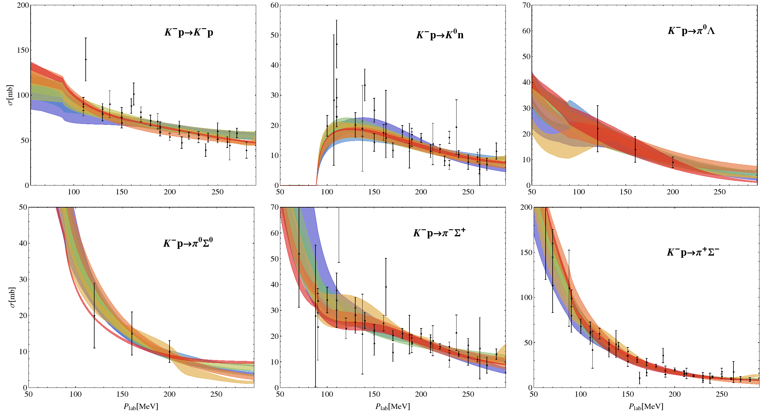
The free parameters of the present model, the low-energy constants as well as the regularization scales are adjusted to reproduce all known experimental data in the meson-baryon sector. The main bulk of this data consists of the cross sections for the processes , , , , , , see Refs. [28, 29, 30, 31]. Here, only data points for the laboratory momentum MeV are considered. Electromagnetic effects are not included in the analysis and assumed to be negligible at the measured values of . At the antikaon-nucleon threshold, we consider the following decay ratios from Refs. [32, 33],
| (3) |
as well as the energy shift and width of kaonic hydrogen in the 1s state, i.e. eV from the SIDDHARTA experiment at DANE [5]. The latter two values are related to the scattering length via the modified Deser-type formula [34]
| (4) |
where is the fine-structure constant, is the reduced mass and the scattering length of the system.

The fit procedure was performed in two steps: First, for randomly chosen starting values of the free parameters (in a natural range) the fit was performed to all threshold values and cross section at a few momenta MeV. Repeating this procedure several thousand times, we ended with several dozen of parameter sets that describe the data equally well. For each of these sets the amplitudes were analytically continued to the positive and negative complex plane. Thereafter, every unphysical solution, e.g. poles on the first Riemann sheet for MeV (), was sorted out. The remaining sets were used in the second step as starting point of the fit procedure, including all threshold and cross section data points, . In both steps the minimizer of the MINUIT2 [35] library was applied on the
where , and denote the number of data points for the observable , the number of parameters and the overall number of observables, respectively. Eight best solutions were obtained by this two-step procedure, see Tab. 1, whereas the next best are at least one order of magnitude larger. Although the fit results look very promising, we would like to point out that there are quite a few free parameters in the model. The latter are assumed to be of natural size, but not restricted otherwise. Thus, we can not exclude that there might be more solutions which describe the assumed experimental data equally well.
2.3 Results
The results of the fits are presented together with the experimental data in Figs. 1 and 2, where every solution is represented by a distinct color. The data are described equally well by all eight solutions, showing, however, different functional behaviour of the cross sections as a function of . These differences are even more pronounced for the scattering amplitude , which is fixed model independently only in the channel at the threshold by the scattering length .
When continued analytically to the complex plane, all eight solutions confirm the double pole structure of the , see Fig. 3. There, the narrow pole lies on the Riemann sheet, connected to the real axis between the thresholds for every solution. The second poles lie on the Riemann sheets, connected to the real axis between the following thresholds: for solution 1, 2, 4, 5 and 8; for solution 3; for solutions 6 and 7. Please note that the second pole of the solution 5 has a shadow pole (5’ in Fig 3) on the Riemann sheet, connected to the real axis between thresholds. The scattering amplitude is restricted around the threshold by the SIDDHARTA measurement quite strongly. Therefore, in the complex plane we observe a very stable behaviour of the amplitude at this energy, i.e. the position of the narrow pole agrees among all solutions within the parameter errors, see Fig. 3. This is in line with the findings of other groups [22, 4, 23], i.e. one observes stability of the position of the narrow pole. Quantitatively, the first pole found in these models is located at somewhat lower energies and is slightly broader than those of our model. In view of the stability of the pole position, we trace this shift to the different treatment of the Born term contributions to the chiral potential utilized in Refs. [22, 4, 23].
The position of the second pole is, on the other hand, less restricted. To be more precise, for the real part we find three clusters of these poles: around the threshold, around the threshold as well as around MeV. For several solutions there is some agreement in the positions of the second pole between the present analysis and the one of Ref. [23] and of our previous work [15]. However, as the experimental data is described similarly well by all fit solutions, one can not reject any of them. Thus, the distribution of poles represents the systematic uncertainty of the present approach. It appears to be quite large, but is still significantly smaller than the older analysis of Ref. [4]. Recall that no restrictions were put on the parameters of the model, except for naturalness.
3 Photoproduction amplitude


In the last section we have demonstrated that the present model for the meson-baryon interaction possess at least eight different solutions, which all describe the hadronic data similarly well. It is therefore of great importance to see how these solutions describe the photoproduction data, if they are considered as final-state interaction of the reaction . To construct such amplitudes one has to extend the framework for one-meson photoproduction, described in Ref. [17], to the production amplitude including two mesons in the final state. As already mentioned in the beginning of the last section such amplitudes would require the full meson-baryon amplitude with the full off-shell dependence. For the chiral potential including contact interactions only, such reactions were studied in Refs. [15, 18, 24], but can also be obtained from the present solution as argued in the last section. Then coupling the photon to every possible place, one obtains a gauge invariant photoproduction amplitude. While such a procedure is straightforward in principle, there are still many technical problems to overcome for the construction of such amplitudes. The goal of the present approach, however, is not the construction of such gauge invariant amplitudes, but to answer the question, whether the new CLAS data allow one to rule out some of the present hadronic solutions. Thus, similar to Refs. [12, 13], we assume the simplest ansatz for the photoproduction amplitude
| (5) |
where and denote the total energy of the system and the invariant mass of the subsystem, respectively. For a specific meson-baryon channel , the energy-dependent (and in general complex valued) constants describe the reaction mechanism of , whereas the final-state interaction is captured by the standard Höhler partial waves . For a specific meson-baryon channel , the Greens function is denoted by and is given by the one-loop meson baryon function in dimensional regularization, i.e. as given in App. B.

The regularization scales appearing in the Eq. (5) via the have already been fixed in the fit to the hadronic cross sections and the SIDDHARTA data. Thus, the only new parameters of the photoproduction amplitude are the constants which, however, are quite numerous (10 for each ). These parameters are adjusted to reproduce the invariant mass distribution for the final , and states and for all 9 measured total energy values GeV. The achieved quality of the photoproduction fits is listed in the third row of Tab. 1, whereas the of the hadronic part are stated in the second row. Note that for the comparison of the photoproduction fits the quantity is not meaningful due to the large number of generic parameters . Therefore, we compare the total divided by the total number of data points for all three final states, denoted by . For the same reason it is not meaningful to perform a global fit, minimizing the total . It turns out that even within such a simple and flexible photoproduction amplitude, only the solutions #2, #4 and #5 of the eight hadronic solutions allows for a decent description of the CLAS data. While the total per data point of these solutions is very close to each other, the next best solution has a 40% larger total than the best one. The failure of the solutions #1, #3, #6, #7 and #8 becomes quite evident in a one-to-one comparison of all eight solutions fitted to the CLAS data as presented in Fig. 6 for one particular cms energy chosen as a typical example. Moreover, the hadronic amplitudes are determined up to 1 error bands. Therefore, it is a priori not clear, whether some of the hadronic solutions lying within these error bands may lead to a better fit of the CLAS data. We have checked this explicitely, considering a large number of hadronic solutions distributed randomly around the central ones. For every such solution a fit to the CLAS data was performed independently and no significanly better fit was found to those of the central solution. Therefore, we consider the above exclusion principle of the hadronic solutions as statistically stable.
| solution | pole 1 | pole 2 |
|---|---|---|
| #2 | ||
| #4 |
The best solution is indeed #4, which we display in Fig. 4. Incidentally, it also has the lowest for the hadronic part. This solution also gives an excellent description of the mass distribution from Ref. [7], calculated using the method developed in Ref. [1], c.f. Fig. 5. With respect to these data, solution #2 is also satisfactory but #5 is not. Therefore, the photoproduction data combined with the scattering and the SIDDHARTA data lead to a sizable reduction in the ambiguity of the second pole of the . In fact, the second pole of the surviving solutions is close to the value found in Ref. [12] (which has, however, no error bars), see Fig. 3, and also close to the central value of the analysis based on scattering data only [4]. To be precise, we give the location of the two poles in these surviving solutions in Tab. 2.
Given the simple phenomenological photoproduction model used here, we do not attempt a full-fledged error analysis of the fits to the CLAS data. However, to get an idea about the uncertainties, we show in Fig. 7 the bands generated from taking the solution within the errors of the hadronic amplitude for solution #4. To be precise, these are not bands for the corresponding curves but some upper limit on the uncertainties of the fits generated from variations in the hadronic amplitude. For a true error analysis of the photoproduction data, one has to work with a truly microscopic model of the photoproduction amplitude, as developed in Refs. [17, 18].
4 Discussion and summary
In the present work we have utilized a chiral unitary approach to construct the amplitude for antikaon-nucleon scattering at NLO in the expansion of the interaction potential. Several sets of fit parameters were found to describe the data similarly well. The two-pole structure of the could be confirmed in each of these solutions. However, while the narrow pole appeared to be quite stable among these solutions, the broad one was found to be distributed in quite large region of the complex W-plane. In the second part of this work we have utilized a simple model, similar to the one of Ref. [12], to demonstrate that one can rule out several hadronic solutions by demanding a good description of the CLAS photoproduction data.
We conclude that the inclusion of the CLAS data as experimental input can serve as a new important constraint on the antikaon-nucleon scattering amplitude. However, for future studies a theoretically more robust model for the two-meson photoproduction amplitude is required. We propose that a generalization of the one-meson photoproduction model, presented in Ref. [17, 18], may be the next logical step for this endevaour.
Acknowledgements
We thank Reinhard Schumacher, Ales Cieply and Peter Bruns for useful communications. This work was supported by the European Community-Research Infrastructure Integrating Activity “Study of Strongly Interacting Matter” (acronym HadronPhysics3, Grant Agreement n. 283286) under the Seventh Framework Programme of EU, by the DFG and NSFC through funds provided to the Collaborative Research Center CRC 110 “Symmteries and the Emergence of Structure in QCD”, and by the DFG (TR 16).
Appendix A Coupling matrices
For the channel indices corresponding to the process , the relevant coupling matrices from the leading and next-to leading order chiral Lagrangian read
where is a set of the channel matrices (e.g. for the physical meson fields) and the are the meson decay constants in the respective channel. Moreover, is obtained from the quark mass matrix via the Gell-Mann-Oakes-Renner relations, and given in terms of the meson masses as follows, .
Appendix B Loop integrals and physical constants
Throughout the present work we use the following numerical values for the masses and the meson decay constants (in GeV):
| , | , | , | , | , |
| , | , | , | ||
| , | , | , | , | , |
| , | , | . |
Due to the on-shell projection of the intermediate mesons and baryons only scalar one-meson-one-baryon loop integrals appear in the context of this work. In dimensional regularization and applying applying the subtraction scheme they take the following form
where is the regularization scale and denotes the meson (baryon) mass. Additionally, the commonly used Källén-function is utilized in the above expression.
Appendix C Numerical results of the threshold values
| Solution | [eV] | |||
|---|---|---|---|---|
| #1 | ||||
| #2 | ||||
| #3 | ||||
| #4 | ||||
| #5 | ||||
| #6 | ||||
| #7 | ||||
| #8 |
References
- (1) J. A. Oller and U.-G. Meißner, Phys. Lett. B 500 (2001) 263. [arXiv:hep-ph/0011146].
- (2) D. Jido, J. A. Oller, E. Oset, A. Ramos, and U.-G. Meißner, Nucl. Phys. A 725 (2003) 181. [arXiv:nucl-th/0303062].
- (3) T. Hyodo and D. Jido, Prog. Part. Nucl. Phys. 67 (2012) 55 [arXiv:1104.4474 [nucl-th]].
- (4) B. Borasoy, U.-G. Meißner and R. Nißler, Phys. Rev. C 74 (2006) 055201, [hep-ph/0606108].
- (5) M. Bazzi, et al., Phys. Lett. B 704 (2011) 113, [arXiv:1105.3090 [nucl-ex]].
- (6) M. Mai, V. Baru, E. Epelbaum, A. Rusetsky arXiv:1411.4881 [nucl-th].
- (7) R. J. Hemingway, Nucl. Phys. B 253 (1985) 742.
- (8) I. Zychor et al., Phys. Lett. B 660 (2008) 167 [arXiv:0705.1039 [nucl-ex]].
- (9) G. Agakishiev et al. [HADES Collaboration], Phys. Rev. C 87 (2013) 025201.
- (10) K. Moriya et al. [CLAS Collaboration], Phys. Rev. C 87 (2013) 3, 035206 [arXiv:1301.5000 [nucl-ex]].
- (11) K. Moriya et al. [CLAS Collaboration], Phys. Rev. Lett. 112, 082004 (2014) [arXiv:1402.2296 [hep-ex]].
- (12) L. Roca and E. Oset, Phys. Rev. C 87 (2013) 5, 055201 [arXiv:1301.5741 [nucl-th]].
- (13) L. Roca and E. Oset, Phys. Rev. C 88 (2013) 5, 055206 [arXiv:1307.5752 [nucl-th]].
- (14) S. X. Nakamura and D. Jido, PTEP 2014 (2014) 023D01 [arXiv:1310.5768 [nucl-th]].
- (15) M. Mai and U.-G. Meißner, Nucl. Phys. A 900 (2013) 51 [arXiv:1202.2030 [nucl-th]].
- (16) D. Rönchen et al., Eur. Phys. J. A 50 (2014) 101 [arXiv:1401.0634 [nucl-th]].
- (17) B. Borasoy, P. C. Bruns, U.-G. Meißner and R. Nissler, Eur. Phys. J. A 34 (2007) 161 [arXiv:0709.3181 [nucl-th]].
- (18) M. Mai, P. C. Bruns and U.-G. Meißner, Phys. Rev. D 86 (2012) 094033 [arXiv:1207.4923 [nucl-th]].
- (19) B. Borasoy, R. Nißler and W. Weise, Eur. Phys. J. A 25 (2005) 79, [hep-ph/0505239].
- (20) J. A. Oller, Eur. Phys. J. A 28 (2006) 63, [hep-ph/0603134].
- (21) Y. Ikeda, T. Hyodo and W. Weise, Phys. Lett. B 706 (2011) 63, [arXiv:1109.3005 [nucl-th]].
- (22) Y. Ikeda, T. Hyodo and W. Weise, Nucl. Phys. A 881 (2012) 98 [arXiv:1201.6549 [nucl-th]].
- (23) Z. H. Guo and J. A. Oller, Phys. Rev. C 87 (2013) 3, 035202 [arXiv:1210.3485 [hep-ph]].
- (24) P. C. Bruns, M. Mai, U.-G. Meißner, Phys. Lett. B697 (2011) 254, [arXiv:nucl-th/1012.2233].
- (25) A. Krause, Helv. Phys. Acta 63 (1990) 3.
- (26) M. Frink and U.-G. Meißner, JHEP 0407 (2004) 028, [arXiv:hep-lat/0404018].
- (27) J. Ruiz de Elvira, C. Ditsche, M. Hoferichter, B. Kubis and U.-G. Meißner, EPJ Web Conf. 73 (2014) 05002.
- (28) J. Ciborowski, et al., J. Phys. G 8 (1982) 13.
- (29) W. E. Humphrey and R. R. Ross, Phys. Rev. 127 (1962) 1305.
- (30) M. Sakitt, T. B. Day, R. G. Glasser, N. Seeman, J. H. Friedman, W. E. Humphrey and R. R. Ross, Phys. Rev. 139 (1965) B719.
- (31) M. B. Watson, M. Ferro-Luzzi and R. D. Tripp, Phys. Rev. 131 (1963) 2248.
- (32) D. N. Tovee, et al., Nucl. Phys. B 33 (1971) 493.
- (33) R. J. Nowak, et al., Nucl. Phys. B 139 (1978) 61.
- (34) U.-G. Meißner, U. Raha and A. Rusetsky, Eur. Phys. J. C 35 (2004) 349, [hep-ph/0402261].
- (35) Minuit2 released in ROOT 5.22/00 [http://lcgapp.cern.ch/project/cls/work-packages/mathlibs/minuit].