跳到论文正文
W Papers独立论文阅读器 arXiv:1411.7720 论文正文 计算阅读时间 · 0%
引用这篇论文根据当前论文元数据生成,正式投稿前建议核对。


License: arXiv.org perpetual non-exclusive license
arXiv:1411.7720v2 [math.NA] 08 Jul 2015

The multiplier method to construct conservative
finite difference schemes for ordinary and partial differential equations

Andy T.S. Wan ††thanks: Department of Mathematics and Statistics, McGill University, Montréal, QC, H3A 0B9, Canada (andy.wan@mcgill.ca)    Alexander Bihlo ††thanks: Department of Mathematics and Statistics, Memorial University of Newfoundland, St. John’s, NL, A1C 5S7, Canada (abihlo@mun.ca)    Jean-Christophe Nave ††thanks: Department of Mathematics and Statistics, McGill University, Montréal, QC, H3A 0B9, Canada (jcnave@math.mcgill.ca)
Abstract

We present the multiplier method of constructing conservative finite difference schemes for ordinary and partial differential equations. Given a system of differential equations possessing conservation laws, our approach is based on discretizing conservation law multipliers and their associated density and flux functions. We show that the proposed discretization is consistent for any order of accuracy when the discrete multiplier has a multiplicative inverse. Moreover, we show that by construction, discrete densities can be exactly conserved. In particular, the multiplier method does not require the system to possess a Hamiltonian or variational structure. Examples, including dissipative problems, are given to illustrate the method. In the case when the inverse of the discrete multiplier becomes singular, consistency of the method is also established for scalar ODEs provided the discrete multiplier and density are zero-compatible.

Key words. conservative, structure preserving, finite difference, finite volume, conservation law, first integral, conservation law multiplier, Euler operator, multiplier method

1 Introduction

In recent decades, structure preserving discretizations have become an important idea in designing numerical methods for differential equations. The central theme is to devise discretizations which preserve at the discrete level certain important structures belonging to the continuous problem.

In the case of ordinary differential equations with a Hamiltonian structure, geometric integrators such as, energy-momentum method [LG75, STW92], symplectic integrators [LR04, HLW06], variational integrators [MW01], Lie group methods [Dor10, Hyd14] and method of invariantization [Olv01, KO04] are a class of discretizations which preserves symplectic structure, first integrals, phase space volume or symmetries at the discrete level. Multi-symplectic methods have also been extended to include partial differential equations possessing a Hamiltonian structure [Bri97, BR06, MPS98].

On the other hand for partial differential equations in divergence form, the well-known finite volume methods [LeV92] naturally preserves conserved quantities in discrete subdomains for the equations. More recently, structure preserving discretizations such as discrete exterior calculus [Hir03, DHLM05], mimetic discretizations [BH06, RS11] and finite element exterior calculus [AFW06, AFW10] put forth complete abstract theories on discretizing equations with a differential complex structure. Specifically, these approaches provide consistency, stability and preservation of the key structures of de Rham cohomology and Hodge theory at the discrete level.

In the present work, we propose a numerical method for ordinary differential equations and partial differential equations which preserves discretely their first integrals, or more generally, their conservation laws. In contrast to geometric integrators or multi-symplectic methods which require the equations to possess a Hamiltonian or variational structure, our approach is based solely on the existence of conservation laws for the given set of differential equations and thus is applicable to virtually any physical system in practice. In particular, this method can be applied to dissipative problems possessing conserved quantities.

For a given system of differential equations with a set of conservation laws, under some mild assumptions on the local solvability of the system, there exists so-called conservation law multipliers which are associated to each conservation law and vice versa [Olv00, BCA10]. This can be viewed as a generalization to the well-known Noether’s theorem for equations derived via a variational principle, in which conservation laws of the Euler-Lagrange equations are associated with variational symmetries and vice versa.

The main idea of our approach, called the multiplier method, is to directly discretize the conservation laws and their associated conservation law multipliers in a manner which is consistent to the given set of differential equations. Moreover, this approach provides a general framework for which discrete densities can be conserved exactly by construction. We emphasize the novelty of the multiplier method is that one can discretize a system of differential equations, which may not be in a conserved form, so that its conserved quantities are simultaneously conserved at the discrete level.

The content of this paper is as follows: First, in Section 2, we provide a brief introduction to conservation law multipliers and the relevant background. Then, we describe our method in Section 3.1 for the case of a scalar partial differential equation, as most of the main ideas are already present in that case. In Section 3.2, we generalize the method to the case when there is the same number of equations as the number of conservation laws. In Section 3.3, we treat the case when there are more equations than the number of conservation laws. In Section 4, we illustrate the multiplier method with various examples and demonstrate discrete preservation of their associated conservation laws; this includes problems which do not readily possess a Hamiltonian or variational structure. Finally in Section 5, we define the zero-compatible condition for scalar ODEs in the case when the inverse of multiplicative discrete multipliers become singular and establish the consistency of the multiplier method in that case.

2 Conservation law of PDEs and conservation law multipliers

Before we describe the construction of conservative schemes for PDEs, we introduce some background for conservation laws of PDEs. First, some notations and definitions. Let ℐ=(0,T)\mathcal{I}=(0,T), 𝒱\mathcal{V} be an open neighborhood of a bounded domain Ω\Omega on ℝn\mathbb{R}^{n} and 𝒰(i)\mathcal{U}^{(i)} be open neighborhoods of ℝm​(n+1)i\mathbb{R}^{m(n+1)^{i}} for i∈ℕi\in\mathbb{N}. We express a kk-th order system of PDEs as a function 𝑭:I×𝒱×𝒰(0)×⋯×𝒰(k)→ℝm\boldsymbol{F}:I\times\mathcal{V}\times\mathcal{U}^{(0)}\times\cdots\times\mathcal{U}^{(k)}\rightarrow\mathbb{R}^{m},

𝑭​[𝒖]t,𝒙:=𝑭⁡(t,𝒙,𝒖⁡(t,𝒙),D1​𝒖​(t,𝒙),…,Dk​𝒖​(t,𝒙))=0,{\boldsymbol{F}}[\boldsymbol{u}]_{t,\boldsymbol{x}}:={\boldsymbol{F}}(t,{\boldsymbol{x}};{\boldsymbol{u}}(t,{\boldsymbol{x}}),D^{1}{\boldsymbol{u}}(t,{\boldsymbol{x}}),\dots,D^{k}{\boldsymbol{u}}(t,{\boldsymbol{x}}))=0,

where t∈It\in I, 𝒙=(x1,…,xn)∈𝒱{\boldsymbol{x}}=(x_{1},\dots,x_{n})\in\mathcal{V} are independent variables and 𝒖:I×𝒱→ℝm{\boldsymbol{u}}:I\times\mathcal{V}\rightarrow\mathbb{R}^{m} are the dependent variables with components 𝒖=(u1,…,um)∈𝒰(0){\boldsymbol{u}}=(u^{1},\dots,u^{m})\in\mathcal{U}^{(0)} and Di​𝒖∈𝒰(i)D^{i}\boldsymbol{u}\in\mathcal{U}^{(i)} are all partial derivatives of 𝒖\boldsymbol{u} up to order ii with respect to t,𝒙t,\boldsymbol{x}, for i=1,…,ki=1,\dots,k. To save writing, we introduced the square bracket notation 𝑭​[𝒖]t,𝒙{\boldsymbol{F}}[\boldsymbol{u}]_{t,\boldsymbol{x}} to denote the value of 𝑭\boldsymbol{F}, depending on t,𝒙,t,\boldsymbol{x}, and 𝒖,D1​𝒖,…,Dk​𝒖\boldsymbol{u},D^{1}\boldsymbol{u},\dots,D^{k}\boldsymbol{u}, evaluated at t,𝒙t,\boldsymbol{x}. If 𝑭\boldsymbol{F} is an analytic normal system11 1 The analyticity condition can be relaxed; see normal, nondegenerate system of PDEs in [Olv00]. [Olv00] for which the Cauchy-Kovalevskaya existence theorem is applicable, then there exist local analytic solutions 𝒖\boldsymbol{u} on ℐ×𝒱\mathcal{I}\times\mathcal{V} which allow us to differentiate 𝒖\boldsymbol{u} as many times as we wish on ℐ×𝒱\mathcal{I}\times\mathcal{V}.

Definition 1.

A ll-th order conservation law of 𝐅\boldsymbol{F} is a divergence expression which vanishes on the solutions of 𝐅\boldsymbol{F},

(​Dt​ψ​[𝒖]t,𝒙+D𝒙⋅ϕ​[𝒖]t,𝒙)​|𝑭​[𝒖]t,𝒙=0=0,{\left.\left(\frac{}{}D_{t}\psi[\boldsymbol{u}]_{t,\boldsymbol{x}}+D_{\boldsymbol{x}}\cdot\boldsymbol{\phi}[\boldsymbol{u}]_{t,\boldsymbol{x}}\right)\frac{}{}\right|_{{\boldsymbol{F}[\boldsymbol{u}]_{t,\boldsymbol{x}}}=0}=0,}

for some density function ψ\psi and flux functions ϕ=(ϕ1,…,ϕn)\boldsymbol{\phi}=(\phi^{1},\dots,\phi^{n}) which are analytic on ℐ×𝒱×𝒰(0)×⋯×𝒰(l)\mathcal{I}\times\mathcal{V}\times\mathcal{U}^{(0)}\times\cdots\times\mathcal{U}^{(l)}.

Here, DtD_{t} is the total derivative with respect to tt and the notation D𝒙⋅ϕD_{\boldsymbol{x}}\cdot\boldsymbol{\phi} means D𝒙⋅ϕ=∑i=1nDxi​ϕiD_{\boldsymbol{x}}\cdot\boldsymbol{\phi}=\sum_{i=1}^{n}D_{x_{i}}\phi^{i}, where DxiD_{x_{i}} is the total derivative with respect to xix_{i}.

Clearly, adding two conservation laws together yields a conservation law and multiplying by a scalar constant also yields a conservation law. So, the set of conservation laws of 𝑭\boldsymbol{F} forms a vector space. However, some conservation laws are not as meaningful as others, for example: density and fluxes which together form differential identities, such as Dt​(ux)+Dx​(ut)=0D_{t}(u_{x})+D_{x}(u_{t})=0, or density and fluxes which are differential consequences of the PDEs 𝑭\boldsymbol{F} itself, such as if ψ\psi and ϕi\phi^{i} are of the form ∑j,𝜶Aj,𝜶​D𝜶​Fj\sum_{j,\boldsymbol{\alpha}}A_{j,\boldsymbol{\alpha}}D_{\boldsymbol{\alpha}}F^{j} for some analytic Aj,𝜶A_{j,\boldsymbol{\alpha}}. These two types of conservation laws are classified as trivial conservation laws of 𝑭\boldsymbol{F}. Since we are interested in non-trivial conservation laws, we “mod out” the trivial conservation laws by considering two conservation laws as equivalent if the difference in their density and fluxes yields a trivial conservation law. It can be shown such relation defines an equivalence relation on the set of conservation laws of 𝑭\boldsymbol{F}.

Definition 2.

An mm-tuple of analytic functions 𝛌:ℐ×𝒱×𝒰(0)×⋯×𝒰(r)→ℝm\boldsymbol{\lambda}:\mathcal{I}\times\mathcal{V}\times\mathcal{U}^{(0)}\times\cdots\times\mathcal{U}^{(r)}\rightarrow\mathbb{R}^{m} is called a rr-th order conservation law multiplier of 𝐅\boldsymbol{F} if there exists a density function ψ\psi and flux functions ϕ\boldsymbol{\phi} which are analytic on ℐ×𝒱×𝒰(0)×⋯×𝒰(l)\mathcal{I}\times\mathcal{V}\times\mathcal{U}^{(0)}\times\cdots\times\mathcal{U}^{(l)} such that,

𝝀​[𝒖]t,𝒙⋅𝑭​[𝒖]t,𝒙=Dt​ψ​[𝒖]t,𝒙+D𝒙⋅ϕ​[𝒖]t,𝒙,{\boldsymbol{\lambda}[\boldsymbol{u}]_{t,\boldsymbol{x}}\cdot\boldsymbol{F}[\boldsymbol{u}]_{t,\boldsymbol{x}}=D_{t}\psi[\boldsymbol{u}]_{t,\boldsymbol{x}}+D_{\boldsymbol{x}}\cdot\boldsymbol{\phi}[\boldsymbol{u}]_{t,\boldsymbol{x}},}

holds on ℐ×𝒱×𝒰(0)×⋯×𝒰(l)\mathcal{I}\times\mathcal{V}\times\mathcal{U}^{(0)}\times\cdots\times\mathcal{U}^{(l)}, where l=m​a​x​(r,k)−1l=max(r,k)-1 and the `​`⋅"``\cdot" symbol denotes the usual dot product.

It follows that the existence of a conservation law multiplier of 𝑭\boldsymbol{F} implies the existence of a conservation law of 𝑭\boldsymbol{F}. The converse is also true if the PDE system 𝑭\boldsymbol{F} is an analytic normal system.

Theorem 1 ([Olv00]).

Let 𝐅\boldsymbol{F} be an analytic normal system and suppose a conservation law of 𝐅\boldsymbol{F} is given by the densities ψ\psi and fluxes ϕ\boldsymbol{\phi}. Then there exists a conservation law multiplier 𝛌\boldsymbol{\lambda} such that,

𝝀​[𝒖]t,𝒙⋅𝑭​[𝒖]t,𝒙=Dt​ψ~​[𝒖]t,𝒙+D𝒙⋅ϕ~​[𝒖]t,𝒙,{\boldsymbol{\lambda}[\boldsymbol{u}]_{t,\boldsymbol{x}}\cdot\boldsymbol{F}[\boldsymbol{u}]_{t,\boldsymbol{x}}=D_{t}\widetilde{\psi}[\boldsymbol{u}]_{t,\boldsymbol{x}}+D_{\boldsymbol{x}}\cdot\widetilde{\boldsymbol{\phi}}[\boldsymbol{u}]_{t,\boldsymbol{x}},}

holds on ℐ×𝒱×𝒰(0)×⋯×𝒰(l)\mathcal{I}\times\mathcal{V}\times\mathcal{U}^{(0)}\times\cdots\times\mathcal{U}^{(l)}, where ψ~\widetilde{\psi} and ϕ~\widetilde{\boldsymbol{\phi}} are equivalent density and fluxes to ψ\psi and ϕ\boldsymbol{\phi}, respectively.

Thus, Theorem 1 provides a recipe to find conservation laws of PDEs. In other words, given a fixed order rr, one can in principle find all conservation law of order rr by first finding the set of conservation law multipliers (which might be empty for a given rr), and then compute their associated densities and fluxes. Conservation law multipliers can be computed by using the method of Euler operator [Olv00, BCA10]. Several techniques on computing the density and fluxes associated with a given conservation law multiplier have also been discussed in [BCA10].

3 Conservative finite difference schemes for PDEs

We now describe the theory on how to use conservation law multipliers and their associated density and fluxes to construct conservative finite difference schemes. For clarity of presentation, we have restricted to the case of a uniform spatial mesh and uniform time step, though in principle, extension to non-uniform grids and curved domains is possible.

The main idea is the following: given a system of partial differential equations with a conservation law, we propose a consistent discretization for the equations by approximating its associated conservation law multipliers, density and fluxes. Moreover, we show the proposed discretization satisfies a discrete divergence theorem. In particular, this implies exact conservation of discrete densities in a manner analogous to the telescoping sum for the finite volume method.

There are three parts in this section. First, we will present the main results in the scalar case. Second, we then generalize to the vectorial case when the number of conservation laws is the same as the number of equations. Finally, we further generalize the vectorial case when the number of conservation laws is less than the number of equations. The case when the number of conservation laws is greater than the number of equations requires a more delicate treatment; we will elaborate in the conclusion.

Notation. In this section, we let ℐτ={kτ:k=0,…,N:=⌊T/τ⌋}\mathcal{I}^{\tau}=\{k\tau:k=0,\dots,N:=\lfloor T/\tau\rfloor\} be uniform time steps and denote τ\tau as the time step size. We denote a uniform mesh Ωh:=Ω∩ℝn,h\Omega^{h}:=\Omega\cap\mathbb{R}^{n,h}, where ℝn,h={h​z→∈ℝn:z→∈ℤn}\mathbb{R}^{n,h}=\{h\vec{z}\in\mathbb{R}^{n}:\vec{z}\in\mathbb{Z}^{n}\} are the lattice points in ℝn\mathbb{R}^{n} and hh is the spatial mesh size. To avoid technicality arising from boundary points of Ω\Omega not being on Ωh\Omega^{h}, we shall assume hh to be sufficiently small such that the discretization error of ∂Ω\partial\Omega with ∂Ωh\partial\Omega^{h} to be negligible. Denote the mesh points of Ωh\Omega^{h} by 𝒙J=(xj1,…,xjn){\boldsymbol{x}}_{J}=(x_{j_{1}},\dots,x_{j_{n}}), where J=(j1,…,jn)∈ℤnJ=(j_{1},\dots,j_{n})\in\mathbb{Z}^{n} is a mesh multi-index if 𝒙J∈Ωh{\boldsymbol{x}}_{J}\in\Omega^{h}. Specifically, given a mesh multi-index JJ, by fixing Ji=(j1,…​ji−1,ji+1,…,jn)J_{i}=(j_{1},\dots j_{i-1},j_{i+1},\dots,j_{n}), then jij_{i} can range over a union of MJiM_{J_{i}} consecutive indices {αJi,l,αJi,l+1,…,βJi,l−1,βJi,l}\{\alpha_{J_{i},l},\alpha_{J_{i},l}+1,\dots,\beta_{J_{i},l}-1,\beta_{J_{i},l}\}, for l=1,…,MJil=1,\dots,M_{J_{i}}; i.e. ji∈⋃l=1MJi{αJi,l,…,βJi,l}j_{i}\in\bigcup_{l=1}^{M_{J_{i}}}\{\alpha_{J_{i},l},\dots,\beta_{J_{i},l}\}. In particular, if Ω\Omega is convex, then MJi=1M_{J_{i}}=1 and αJi≤ji≤βJi\alpha_{J_{i}}\leq j_{i}\leq\beta_{J_{i}}. Thus, the boundary of Ωh\Omega^{h} can then be defined as,

∂Ωh=⋃i=1n{𝒙J∈Ωh:J=(j1,…,jn) such that for some l∈{1,…,MJi},ji=αJi,l or βJi,l}.\partial\Omega^{h}=\bigcup_{i=1}^{n}\{\boldsymbol{x}_{J}\in\Omega^{h}:J=(j_{1},\dots,j_{n})\text{ such that for some }l\in\{1,\dots,M_{J_{i}}\},j_{i}=\alpha_{J_{i},l}\text{ or }\beta_{J_{i},l}\}. (1)

We use i^\hat{i} to denote the multi-index (0,…,1,…,0)(0,\dots,1,\dots,0) with 11 at the ii-th component.

Since finite difference discretizations are expressions which depend on values defined on mesh points, we denote the collection of mesh values of a discrete function 𝒖τ,h:ℐτ×Ωh→ℝm\boldsymbol{u}^{\tau,h}:\mathcal{I}^{\tau}\times\Omega^{h}\rightarrow\mathbb{R}^{m} as,

{𝒖τ,h}:=(…,𝒖k+1,J,…,𝒖k,J+i^,𝒖k,J,𝒖k,J−i^,…,𝒖k−1,J,…),\{\boldsymbol{u}^{\tau,h}\}:=(\dots,\boldsymbol{u}_{k+1,J},\dots,\boldsymbol{u}_{k,J+\hat{i}},\boldsymbol{u}_{k,J},\boldsymbol{u}_{k,J-\hat{i}},\dots,\boldsymbol{u}_{k-1,J},\dots),

and denote a finite difference discretization 𝑭τ,h\boldsymbol{F}^{\tau,h} depending on {𝒖τ,h}\{\boldsymbol{u}^{\tau,h}\} at tk,𝒙Jt_{k},\boldsymbol{x}_{J} as,

𝑭τ,h​{𝒖τ,h}k,J:=𝑭τ,h​(tk,𝒙J,…,𝒖k+1,J,…,𝒖k,J+i^,𝒖k,J,𝒖k,J−i^,…,𝒖k−1,J,…).\boldsymbol{F}^{\tau,h}\{\boldsymbol{u}^{\tau,h}\}_{k,J}:=\boldsymbol{F}^{\tau,h}(t_{k},\boldsymbol{x}_{J};\dots,\boldsymbol{u}_{k+1,J},\dots,\boldsymbol{u}_{k,J+\hat{i}},\boldsymbol{u}_{k,J},\boldsymbol{u}_{k,J-\hat{i}},\dots,\boldsymbol{u}_{k-1,J},\dots).

In order to discuss the consistency of finite difference discretization for 𝑭τ,h\boldsymbol{F}^{\tau,h}, we also denote the expression of 𝑭τ,h\boldsymbol{F}^{\tau,h} when evaluated on the mesh values of any continuous function 𝒖∈C⁡(ℐ×Ω¯)\boldsymbol{u}\in C(\overline{\mathcal{I}\times\Omega}) as,

𝑭τ,h​{𝒖}tk,𝒙J:=𝑭τ,h​(tk,𝒙J,…,𝒖⁡(tk+1,𝒙J),…,𝒖⁡(tk,𝒙J+i^),𝒖⁡(tk,𝒙J),𝒖⁡(tk,𝒙J−i^),…,𝒖⁡(tk−1,𝒙J),…).\boldsymbol{F}^{\tau,h}\{\boldsymbol{u}\}_{t_{k},\boldsymbol{x}_{J}}:=\boldsymbol{F}^{\tau,h}(t_{k},\boldsymbol{x}_{J};\dots,\boldsymbol{u}(t_{k+1},\boldsymbol{x}_{J}),\dots,\boldsymbol{u}(t_{k},\boldsymbol{x}_{J+\hat{i}}),\boldsymbol{u}(t_{k},\boldsymbol{x}_{J}),\boldsymbol{u}(t_{k},\boldsymbol{x}_{J-\hat{i}}),\dots,\boldsymbol{u}(t_{k-1},\boldsymbol{x}_{J}),\dots).

Similarly, we shall use the same notations for finite difference discretizations of multipliers 𝝀τ,h\boldsymbol{\lambda}^{\tau,h}, total derivative of the density Dtτ,h​ψD_{t}^{\tau,h}\psi and total derivative of the fluxes D𝒙τ,h​ϕD_{\boldsymbol{x}}^{\tau,h}\boldsymbol{\phi}. Often to save writing, we will omit the subscripts k,Jk,J or tk,𝒙Jt_{k},\boldsymbol{x}_{J} when the specific mesh point is clear from the context.

3.1 Scalar PDE with one conservation law

We first consider the scalar case when 𝒖\boldsymbol{u} has only one component uu,

F​[u]t,𝒙=0, in ​t∈ℐ,𝒙∈Ω,F[u]_{t,\boldsymbol{x}}=0,\text{ in }t\in\mathcal{I},{\boldsymbol{x}}\in\Omega, (2)

with one conservation law. In particular, we have a conservation law multiplier λ\lambda with their associated densities ψ\psi and fluxes ϕ{\boldsymbol{\phi}} satisfying,

λ​[u]t,𝒙⋅F​[u]t,𝒙=Dt​ψ​[u]t,𝒙+D𝒙⋅ϕ​[u]t,𝒙.\lambda[u]_{t,\boldsymbol{x}}\cdot F[u]_{t,\boldsymbol{x}}=D_{t}\psi[u]_{t,\boldsymbol{x}}+D_{\boldsymbol{x}}\cdot{\boldsymbol{\phi}}[u]_{t,\boldsymbol{x}}.
Theorem 2.

Let u∈Cmax⁡(p,q)+max⁡(r,k)​(ℐ×Ω¯)u\in C^{\max(p,q)+\max(r,k)}(\overline{\mathcal{I}\times\Omega})22 2 Recall, we assumed λ\lambda has up to rr-th order derivatives and FF has up to kk-th order derivatives. Moreover, additional max⁡(p,q)\max(p,q) derivatives are necessary to state consistency for λτ,h\lambda^{\tau,h}, Dtτ,h​ψD^{\tau,h}_{t}\psi and D𝐱τ,h⋅ϕD_{\boldsymbol{x}}^{\tau,h}\cdot\boldsymbol{\phi} required for the use of Taylor’s Theorem. and λ\lambda be a conservation law multiplier of (2) with corresponding density ψ\psi and fluxes ϕ\boldsymbol{\phi}. Suppose λτ,h\lambda^{\tau,h}, Dtτ,h​ψD_{t}^{\tau,h}\psi and D𝐱τ,h⋅ϕD_{\boldsymbol{x}}^{\tau,h}\cdot\boldsymbol{\phi} are finite difference discretizations of λ\lambda, Dt​ψD_{t}\psi and D𝐱⋅ϕD_{\boldsymbol{x}}\cdot\boldsymbol{\phi} with accuracy up to order pp in space and qq in time:

‖λ⁡[u]−λτ,h​{u}‖l∞​(ℐτ×Ωh)\displaystyle\left\lVert\lambda[u]-\lambda^{\tau,h}\{u\}\right\rVert_{l^{\infty}(\mathcal{I}^{\tau}\times\Omega^{h})} ≤Cλ​(hp+τq),\displaystyle\leq C_{\lambda}(h^{p}+\tau^{q}),
‖Dt​ψ​[u]−Dtτ,h​ψ​{u}‖l∞​(ℐτ×Ωh)\displaystyle\left\lVert D_{t}\psi[u]-D_{t}^{\tau,h}\psi\{u\}\right\rVert_{l^{\infty}(\mathcal{I}^{\tau}\times\Omega^{h})} ≤Ct​(hp+τq),\displaystyle\leq C_{t}(h^{p}+\tau^{q}),
‖D𝒙⋅ϕ⁡[u]−D𝒙τ,h⋅ϕ⁡{u}‖l∞​(ℐτ×Ωh)\displaystyle\left\lVert D_{\boldsymbol{x}}\cdot\boldsymbol{\phi}[u]-D_{\boldsymbol{x}}^{\tau,h}\cdot\boldsymbol{\phi}\{u\}\right\rVert_{l^{\infty}(\mathcal{I}^{\tau}\times\Omega^{h})} ≤Cx​(hp+τq).\displaystyle\leq C_{x}(h^{p}+\tau^{q}).

Let uτ,h:ℐτ×Ωh→ℝu^{\tau,h}:\mathcal{I}^{\tau}\times\Omega^{h}\rightarrow\mathbb{R} be a discrete scalar function. Suppose (λτ,h)−1​{uτ,h}{(\lambda^{\tau,h})}^{-1}\{u^{\tau,h}\}, the multiplicative inverse of λτ,h​{uτ,h}\lambda^{\tau,h}\{u^{\tau,h}\}, exists on ℐτ×Ωh\mathcal{I}^{\tau}\times\Omega^{h} and that ‖(λτ,h)−1​{uτ,h}‖l∞​(ℐτ×Ωh)≤γ<∞\left\lVert{(\lambda^{\tau,h})}^{-1}\{u^{\tau,h}\}\right\rVert_{l^{\infty}(\mathcal{I}^{\tau}\times\Omega^{h})}\leq\gamma<\infty, with γ\gamma independent of τ,h\tau,h. Define the finite difference discretization of FF as,

Fτ,h​{uτ,h}:=(λτ,h)−1​{uτ,h}​(Dtτ,h​ψ​{uτ,h}+D𝒙τ,h⋅ϕ⁡{uτ,h}).F^{\tau,h}\{u^{\tau,h}\}:={(\lambda^{\tau,h})}^{-1}\{u^{\tau,h}\}\left(D_{t}^{\tau,h}\psi\{u^{\tau,h}\}+D_{\boldsymbol{x}}^{\tau,h}\cdot\boldsymbol{\phi}\{u^{\tau,h}\}\right). (3)

Then there exists a constant C>0C>0 independent of h,τh,\tau such that,

‖F⁡[u]−Fτ,h​{u}‖l∞​(ℐτ×Ωh)≤C⁡(hp+τq)\left\lVert F[u]-F^{\tau,h}\{u\}\right\rVert_{l^{\infty}(\mathcal{I}^{\tau}\times\Omega^{h})}\leq C(h^{p}+\tau^{q})
Proof.

Fix (tk,𝒙J)∈ℐτ×Ωh(t_{k},\boldsymbol{x}_{J})\in\mathcal{I}^{\tau}\times\Omega^{h}. Since λ\lambda is a conservation law multiplier of FF and by definition of Fτ,hF^{\tau,h},

F⁡[u]\displaystyle F[u] −Fτ,h​{u}\displaystyle-F^{\tau,h}\{u\}
=(λτ,h)−1​{u}​(λτ,h​{u}​F​[u]−Dtτ,h​ψ​{u}−D𝒙τ,h⋅ϕ⁡{u})\displaystyle={(\lambda^{\tau,h})}^{-1}\{u\}\left(\lambda^{\tau,h}\{u\}F[u]-D_{t}^{\tau,h}\psi\{u\}-D_{\boldsymbol{x}}^{\tau,h}\cdot\boldsymbol{\phi}\{u\}\right)
=(λτ,h)−1​{u}​((λτ,h​{u}−λ⁡[u])​F​[u]+(Dt​ψ​[u]−Dtτ,h​ψ​{u})+(D𝒙⋅ϕ⁡[u]−D𝒙τ,h⋅ϕ⁡{u}))\displaystyle={(\lambda^{\tau,h})}^{-1}\{u\}\left((\lambda^{\tau,h}\{u\}-\lambda[u])F[u]+\left(D_{t}\psi[u]-D_{t}^{\tau,h}\psi\{u\}\right)+\left(D_{\boldsymbol{x}}\cdot\boldsymbol{\phi}[u]-D_{\boldsymbol{x}}^{\tau,h}\cdot\boldsymbol{\phi}\{u\}\right)\right) (4)

Since u∈Cmax⁡(p,q)+max⁡(r,k)​(ℐ×Ω¯)u\in C^{\max(p,q)+\max(r,k)}(\overline{\mathcal{I}\times\Omega}) and F⁡[u]F[u] is continuous in its arguments, F​[u]t,𝒙F[u]_{t,\boldsymbol{x}} is continuous on ℐ×Ω¯\overline{\mathcal{I}\times\Omega} and thus |F​[u]t,𝒙|≤C′|F[u]_{t,\boldsymbol{x}}|\leq C^{\prime} uniformly on ℐ×Ω¯\overline{\mathcal{I}\times\Omega}. By (4),

|F⁡[u]−Fτ,h​{u}|\displaystyle\left|F[u]-F^{\tau,h}\{u\}\right| ≤|(λτ,h)−1​{u}|​(|λτ,h​{u}−λ⁡[u]|​|F⁡[u]|+|Dt​ψ​[u]−Dtτ,h​ψ​{u}|+|D𝒙⋅ϕ⁡[u]−D𝒙τ,h⋅ϕ⁡{u}|)\displaystyle\leq|{(\lambda^{\tau,h})}^{-1}\{u\}|\left(\left|\lambda^{\tau,h}\{u\}-\lambda[u]\right||F[u]|+\left|D_{t}\psi[u]-D_{t}^{\tau,h}\psi\{u\}\right|+\left|D_{\boldsymbol{x}}\cdot\boldsymbol{\phi}[u]-D_{\boldsymbol{x}}^{\tau,h}\cdot\boldsymbol{\phi}\{u\}\right|\right)
OPEN≤γ⁡(C′​Cλ​(hp+τq))+Ct​(hp+τq)+Cx​(hp+τq))=C⁡(hp+τq),\displaystyle\leq\gamma(C^{\prime}C_{\lambda}(h^{p}+\tau^{q}))+C_{t}(h^{p}+\tau^{q})+C_{x}(h^{p}+\tau^{q}))=C(h^{p}+\tau^{q}), (5)

where C:=γ⁡(C′​Cλ+Ct+Cx)\displaystyle C:=\gamma\left(C^{\prime}C_{\lambda}+C_{t}+C_{x}\right). Since this is true for arbitrary mesh points (tk,𝒙J)∈ℐτ×Ωh(t_{k},\boldsymbol{x}_{J})\in\mathcal{I}^{\tau}\times\Omega^{h}, taking the maximum of (5) over all points in ℐτ×Ωh\mathcal{I}^{\tau}\times\Omega^{h} gives the desired result.

∎

In other words, Theorem 2 says the discretization given by (3) is a consistent discretization of (2), provided λτ,h​{uτ,h}\lambda^{\tau,h}\{u^{\tau,h}\} does not vanish on some (tk,𝒙J)∈ℐτ×Ωh(t_{k},\boldsymbol{x}_{J})\in\mathcal{I}^{\tau}\times\Omega^{h}. We will return in Section 5 to address the issue of when λτ,h​{uτ,h}\lambda^{\tau,h}\{u^{\tau,h}\} do vanish. Next we show that the finite difference discretization Fτ,hF^{\tau,h} is conservative in the following sense.

Theorem 3.

Let λ\lambda be a conservation law multiplier of (2) with density ψ\psi and fluxes ϕ\boldsymbol{\phi} and let λτ,h\lambda^{\tau,h} be a finite difference discretizations of λ\lambda. Let uτ,h:ℐτ×Ωh→ℝu^{\tau,h}:\mathcal{I}^{\tau}\times\Omega^{h}\rightarrow\mathbb{R} be a discrete scalar function. Define Dtτ,h​ψD_{t}^{\tau,h}\psi and D𝐱τ,h⋅ϕD_{\boldsymbol{x}}^{\tau,h}\cdot\boldsymbol{\phi} to be the following discretizations,

Dtτ,h​ψ​{uτ,h}k,J\displaystyle D_{t}^{\tau,h}\psi\{u^{\tau,h}\}_{k,J} =ψτ,h​{uτ,h}k,J−ψτ,h​{uτ,h}k−1,Jτ,\displaystyle=\frac{\psi^{\tau,h}\{u^{\tau,h}\}_{k,J}-\psi^{\tau,h}\{u^{\tau,h}\}_{k-1,J}}{\tau}, (6a)
D𝒙τ,h⋅ϕ​{uτ,h}k,J\displaystyle D_{\boldsymbol{x}}^{\tau,h}\cdot\boldsymbol{\phi}\{u^{\tau,h}\}_{k,J} =∑i=1nϕi,τ,h​{uτ,h}k,J−ϕi,τ,h​{uτ,h}k,J−i^h,\displaystyle=\sum_{i=1}^{n}\frac{\phi^{i,\tau,h}\{u^{\tau,h}\}_{k,J}-\phi^{i,\tau,h}\{u^{\tau,h}\}_{k,J-\hat{i}}}{h}, (6b)

where ψτ,h\psi^{\tau,h} and ϕi,τ,h\phi^{i,\tau,h} are finite difference discretizations of ψ\psi and ϕi\phi^{i}. Also let Fτ,hF^{\tau,h} be the corresponding discretization of (2) given by (3). If uτ,hu^{\tau,h} is a solution to the discrete problem,

Fτ,h​{uτ,h}k,J=0,𝒙J∈Ωh,F^{\tau,h}\{u^{\tau,h}\}_{k,J}=0,\hskip 8.53581pt{\boldsymbol{x}}_{J}\in\Omega^{h}, (7)

then the discrete divergence theorem for uτ,hu^{\tau,h} holds,

0=1τ​∑𝒙J∈Ωh(ψτ,h​{uτ,h}k,J−ψτ,h​{uτ,h}k−1,J)+1h​∑𝒙J∈∂Ωhϕτ,h​{uτ,h}k,J⋅𝝂J,\displaystyle 0=\frac{1}{\tau}\sum_{{\boldsymbol{x}}_{J}\in\Omega^{h}}\left(\psi^{\tau,h}\{u^{\tau,h}\}_{k,J}-\psi^{\tau,h}\{u^{\tau,h}\}_{k-1,J}\right)+\frac{1}{h}\sum_{{\boldsymbol{x}}_{J}\in\partial\Omega^{h}}\boldsymbol{\phi}^{\tau,h}\{u^{\tau,h}\}_{k,J}\cdot\boldsymbol{\nu}^{J},

where 𝛎J=(ν1J,…,νnJ)\boldsymbol{\nu}^{J}=(\nu_{1}^{J},\dots,\nu_{n}^{J}) is the outward-pointing unit normal of ∂Ωh\partial\Omega^{h} at 𝐱J\boldsymbol{x}_{J}.

Proof.

Since uτ,hu^{\tau,h} satisfies (7) for all 𝒙J∈Ωh\boldsymbol{x}_{J}\in\Omega^{h} and by definition of Fτ,hF^{\tau,h},

0\displaystyle 0 =∑𝒙J∈Ωhλτ,h​{uτ,h}k,J​Fτ,h​{uτ,h}k,J=∑𝒙J∈Ωh(Dtτ,h​ψ​{uτ,h}k,J)+∑𝒙J∈Ωh(D𝒙τ,h⋅ϕ​{uτ,h}k,J)\displaystyle=\sum_{{\boldsymbol{x}}_{J}\in\Omega^{h}}\lambda^{\tau,h}\{u^{\tau,h}\}_{k,J}F^{\tau,h}\{u^{\tau,h}\}_{k,J}=\sum_{{\boldsymbol{x}}_{J}\in\Omega^{h}}\left(D_{t}^{\tau,h}\psi\{u^{\tau,h}\}_{k,J}\right)+\sum_{{\boldsymbol{x}}_{J}\in\Omega^{h}}\left(D_{\boldsymbol{x}}^{\tau,h}\cdot\boldsymbol{\phi}\{u^{\tau,h}\}_{k,J}\right)
=1τ​∑𝒙J∈Ωh(ψτ,h​{uτ,h}k,J−ψτ,h​{uτ,h}k−1,J)+1h​∑i=1n∑𝒙J∈Ωh(ϕi,τ,h​{uτ,h}k,J−ϕi,τ,h​{uτ,h}k,J−i^).\displaystyle=\frac{1}{\tau}\sum_{{\boldsymbol{x}}_{J}\in\Omega^{h}}\left(\psi^{\tau,h}\{u^{\tau,h}\}_{k,J}-\psi^{\tau,h}\{u^{\tau,h}\}_{k-1,J}\right)+\frac{1}{h}\sum_{i=1}^{n}\sum_{{\boldsymbol{x}}_{J}\in\Omega^{h}}\left(\phi^{i,\tau,h}\{u^{\tau,h}\}_{k,J}-\phi^{i,\tau,h}\{u^{\tau,h}\}_{k,J-\hat{i}}\right). (8)

For each fixed ii and Ji=(j1,…,ji−1,ji+1,…​jn)J_{i}=(j_{1},\dots,j_{i-1},j_{i+1},\dots j_{n}), recall that ji∈⋃l=1MJi{αJi,l,…,βJi,l}j_{i}\in\bigcup_{l=1}^{M_{J_{i}}}\{\alpha_{J_{i},l},\dots,\beta_{J_{i},l}\}. Thus,

∑𝒙J∈Ωh(ϕi,τ,h​{uτ,h}k,J−ϕi,τ,h​{uτ,h}k,J−i^)=∑j1,…,jn(ϕi,τ,h​{uτ,h}k,(j1,…,ji,…,jn)−ϕi,τ,h​{uτ,h}k,(j1,…,ji−1,…,jn))\displaystyle\sum_{{\boldsymbol{x}}_{J}\in\Omega^{h}}\left(\phi^{i,\tau,h}\{u^{\tau,h}\}_{k,J}-\phi^{i,\tau,h}\{u^{\tau,h}\}_{k,J-\hat{i}}\right)=\sum_{\begin{subarray}{c}j_{1},\dots,j_{n}\end{subarray}}\left(\phi^{i,\tau,h}\{u^{\tau,h}\}_{k,(j_{1},\dots,j_{i},\dots,j_{n})}-\phi^{i,\tau,h}\{u^{\tau,h}\}_{k,(j_{1},\dots,j_{i}-1,\dots,j_{n})}\right)
=∑j1,…,ji−1,ji+1,…,jn∑l=1MJi∑ji=αJi,l+1βJi,l(ϕi,τ,h​{uτ,h}k,(j1,…,ji,…,jn)−ϕi,τ,h​{uτ,h}k,(j1,…,ji−1,…,jn))\displaystyle=\sum_{j_{1},\dots,j_{i-1},j_{i+1},\dots,j_{n}}\sum_{l=1}^{M_{J_{i}}}\sum_{j_{i}=\alpha_{J_{i},l}+1}^{\beta_{J_{i},l}}\left(\phi^{i,\tau,h}\{u^{\tau,h}\}_{k,(j_{1},\dots,j_{i},\dots,j_{n})}-\phi^{i,\tau,h}\{u^{\tau,h}\}_{k,(j_{1},\dots,j_{i}-1,\dots,j_{n})}\right)
=∑j1,…,ji−1,ji+1,…,jn∑l=1MJi(ϕi,τ,h​{uτ,h}k,(j1,…,βJi,l,…,jn)−ϕi,τ,h​{uτ,h}k,(j1,…,αJi,l,…,jn))\displaystyle=\sum_{j_{1},\dots,j_{i-1},j_{i+1},\dots,j_{n}}\sum_{l=1}^{M_{J_{i}}}\left(\phi^{i,\tau,h}\{u^{\tau,h}\}_{k,(j_{1},\dots,\beta_{J_{i},l},\dots,j_{n})}-\phi^{i,\tau,h}\{u^{\tau,h}\}_{k,(j_{1},\dots,\alpha_{J_{i},l},\dots,j_{n})}\right)
=∑𝒙J∈Ωhji∈⋃l=1MJi{αJi,l,βJi,l}ϕi,τ,h​{uτ,h}k,J​νiJ.\displaystyle=\sum_{\begin{subarray}{c}{\boldsymbol{x}}_{J}\in\Omega^{h}\\ j_{i}\in\bigcup_{l=1}^{M_{J_{i}}}\{\alpha_{J_{i},l},\beta_{J_{i},l}\}\end{subarray}}\phi^{i,\tau,h}\{u^{\tau,h}\}_{k,J}\nu_{i}^{J}.

And so (8) implies

0\displaystyle 0 =1τ​∑𝒙J∈Ωh(ψτ,h​{uτ,h}k,J−ψτ,h​{uτ,h}k−1,J)+1h​∑i=1n∑𝒙J∈Ωhji∈⋃l=1MJi{αJi,l,βJi,l}ϕi,τ,h​{uτ,h}k,J​νiJ\displaystyle=\frac{1}{\tau}\sum_{{\boldsymbol{x}}_{J}\in\Omega^{h}}\left(\psi^{\tau,h}\{u^{\tau,h}\}_{k,J}-\psi^{\tau,h}\{u^{\tau,h}\}_{k-1,J}\right)+\frac{1}{h}\sum_{i=1}^{n}\sum_{\begin{subarray}{c}{\boldsymbol{x}}_{J}\in\Omega^{h}\\ j_{i}\in\bigcup_{l=1}^{M_{J_{i}}}\{\alpha_{J_{i},l},\beta_{J_{i},l}\}\end{subarray}}\phi^{i,\tau,h}\{u^{\tau,h}\}_{k,J}\nu_{i}^{J}
=1τ​∑𝒙J∈Ωh(ψτ,h​{uτ,h}k,J−ψτ,h​{uτ,h}k−1,J)+1h​∑𝒙J∈∂Ωhϕτ,h​{uτ,h}k,J⋅𝝂J,\displaystyle=\frac{1}{\tau}\sum_{{\boldsymbol{x}}_{J}\in\Omega^{h}}\left(\psi^{\tau,h}\{u^{\tau,h}\}_{k,J}-\psi^{\tau,h}\{u^{\tau,h}\}_{k-1,J}\right)+\frac{1}{h}\sum_{{\boldsymbol{x}}_{J}\in\partial\Omega^{h}}\boldsymbol{\phi}^{\tau,h}\{u^{\tau,h}\}_{k,J}\cdot\boldsymbol{\nu}^{J},

where the last equality follows from definition of ∂Ωh\partial\Omega^{h} in (1). ∎

Although it may appear that Theorem 3 restricts the discrete density and fluxes to be first order accurate, it is possible to obtain higher order accuracy for the density and fluxes, as we will illustrate in the examples.

Corollary 1.

Let ψτ,h,ϕτ,h\psi^{\tau,h},\boldsymbol{\phi}^{\tau,h} be as given in Theorem 3 and the discrete scalar function uτ,h:ℐτ×Ωh→ℝu^{\tau,h}:\mathcal{I}^{\tau}\times\Omega^{h}\rightarrow\mathbb{R} be a solution to (7) at tkt_{k}. If the discretized fluxes ϕτ,h​{uτ,h}\boldsymbol{\phi}^{\tau,h}\{u^{\tau,h}\} vanish on the boundary ∂Ωh\partial\Omega^{h}, then

∑𝒙J∈Ωhψτ,h​{uτ,h}k,J=∑𝒙J∈Ωhψτ,h​{uτ,h}k−1,J.\displaystyle\sum_{{\boldsymbol{x}}_{J}\in\Omega^{h}}\psi^{\tau,h}\{u^{\tau,h}\}_{k,J}=\sum_{{\boldsymbol{x}}_{J}\in\Omega^{h}}\psi^{\tau,h}\{u^{\tau,h}\}_{k-1,J}.

In other words, the proposed scheme has exact discrete conservation.

3.2 System of mm PDEs with mm conservation laws

Next we extend the previous results to systems of PDEs. Consider a kk-th order system of mm PDEs,

𝑭​[𝒖]t,𝒙=0, on ​t∈ℐ,𝒙∈Ω,{\boldsymbol{F}}[\boldsymbol{u}]_{t,\boldsymbol{x}}=0,\text{ on }t\in\mathcal{I},{\boldsymbol{x}}\in\Omega, (9)

with mm conservation laws. In particular, we have an m×mm\times m matrix of conservation law multipliers Λ​[𝒖]t,𝒙\Lambda[\boldsymbol{u}]_{t,\boldsymbol{x}},

Λ​[𝒖]t,𝒙=(λ11​[𝒖]t,𝒙…λ1​m​[𝒖]t,𝒙λm​1​[𝒖]t,𝒙…λm​m​[𝒖]t,𝒙),\Lambda[\boldsymbol{u}]_{t,\boldsymbol{x}}=\begin{pmatrix}\lambda^{11}[\boldsymbol{u}]_{t,\boldsymbol{x}}&\dots&\lambda^{1m}[\boldsymbol{u}]_{t,\boldsymbol{x}}\\ \vdots&&\vdots\\ \lambda^{m1}[\boldsymbol{u}]_{t,\boldsymbol{x}}&\dots&\lambda^{mm}[\boldsymbol{u}]_{t,\boldsymbol{x}}\\ \end{pmatrix}, (10)

with their associated densities 𝝍​[𝒖]t,𝒙\boldsymbol{\psi}[\boldsymbol{u}]_{t,\boldsymbol{x}} and fluxes Φ​[𝒖]t,𝒙\Phi[\boldsymbol{u}]_{t,\boldsymbol{x}},

𝝍​[𝒖]t,𝒙=(ψ1​[𝒖]t,𝒙ψm​[𝒖]t,𝒙),\displaystyle\boldsymbol{\psi}[\boldsymbol{u}]_{t,\boldsymbol{x}}=\begin{pmatrix}\psi^{1}[\boldsymbol{u}]_{t,\boldsymbol{x}}\\ \vdots\\ \psi^{m}[\boldsymbol{u}]_{t,\boldsymbol{x}}\\ \end{pmatrix}, ​Φ​[𝒖]t,𝒙=(ϕ11​[𝒖]t,𝒙…ϕ1​n​[𝒖]t,𝒙ϕm​1​[𝒖]t,𝒙…ϕm​n​[𝒖]t,𝒙),\displaystyle\text{ }{\Phi[\boldsymbol{u}]_{t,\boldsymbol{x}}=\begin{pmatrix}\phi^{11}[\boldsymbol{u}]_{t,\boldsymbol{x}}&\dots&\phi^{1n}[\boldsymbol{u}]_{t,\boldsymbol{x}}\\ \vdots&&\vdots\\ \phi^{m1}[\boldsymbol{u}]_{t,\boldsymbol{x}}&\dots&\phi^{mn}[\boldsymbol{u}]_{t,\boldsymbol{x}}\\ \end{pmatrix}}, (11)

satisfying,

Λ​[𝒖]t,𝒙⋅𝑭​[𝒖]t,𝒙=Dt​𝝍​[𝒖]t,𝒙+D𝒙⋅Φ​[𝒖]t,𝒙.\Lambda[\boldsymbol{u}]_{t,\boldsymbol{x}}\cdot\boldsymbol{F}[\boldsymbol{u}]_{t,\boldsymbol{x}}=D_{t}\boldsymbol{\psi}[\boldsymbol{u}]_{t,\boldsymbol{x}}+D_{\boldsymbol{x}}\cdot\Phi[\boldsymbol{u}]_{t,\boldsymbol{x}}.

Here the notation D𝒙⋅ΦD_{\boldsymbol{x}}\cdot\Phi is analogous to the divergence applied to the tensor Φ\Phi, i.e. (D𝒙⋅Φ)j=∑j=1nDxi​ϕj​i(D_{\boldsymbol{x}}\cdot\Phi)^{j}=\sum_{j=1}^{n}D_{x_{i}}\phi^{ji}.

Analogous to (3), we now show the following discretization of the system of PDEs is consistent provided the discrete multiplier matrix Λτ,h​{𝒖τ,h}k,J\Lambda^{\tau,h}\{\boldsymbol{u}^{\tau,h}\}_{k,J} is invertible on ℐτ×Ωh\mathcal{I}^{\tau}\times\Omega^{h} and ‖‖(Λτ,h)−1​{𝒖τ,h}‖o​p‖l∞​(ℐτ×Ωh)\displaystyle\left\lVert\left\lVert\left({\Lambda^{\tau,h}}\right)^{-1}\{\boldsymbol{u}^{\tau,h}\}\right\rVert_{op}\right\rVert_{l^{\infty}(\mathcal{I}^{\tau}\times\Omega^{h})} is bounded above uniformly in τ,h\tau,h, where ‖⋅‖o​p\left\lVert\cdot\right\rVert_{op} is the induced matrix norm of the vector norm |⋅||\cdot|.

Theorem 4.

Let 𝐮∈Cmax⁡(p,q)+max⁡(r,k)​(ℐ×Ω¯)\boldsymbol{u}\in C^{\max(p,q)+\max(r,k)}(\overline{\mathcal{I}\times\Omega}) and Λ\Lambda in (10) be an m×mm\times m matrix of conservation law multipliers of (9) with corresponding density 𝛙\boldsymbol{\psi} and fluxes Φ\Phi, as defined in (11). Suppose Λτ,h\Lambda^{\tau,h}, Dtτ,h​𝛙D_{t}^{\tau,h}\boldsymbol{\psi} and D𝐱τ,h⋅ΦD_{\boldsymbol{x}}^{\tau,h}\cdot\Phi are finite difference discretizations of Λ\Lambda, Dt​𝛙D_{t}\boldsymbol{\psi} and D𝐱⋅ΦD_{\boldsymbol{x}}\cdot\Phi with accuracy up to order pp in space and qq in time:

‖‖Λ⁡[𝒖]−Λτ,h​{𝒖}‖o​p‖l∞​(ℐτ×Ωh)\displaystyle\left\lVert\left\lVert\Lambda[\boldsymbol{u}]-\Lambda^{\tau,h}\{\boldsymbol{u}\}\right\rVert_{op}\right\rVert_{l^{\infty}(\mathcal{I}^{\tau}\times\Omega^{h})} ≤CΛ​(hp+τq),\displaystyle\leq C_{\Lambda}(h^{p}+\tau^{q}),
‖Dt​𝝍​[𝒖]−Dtτ,h​𝝍​{𝒖}‖l∞​(ℐτ×Ωh)\displaystyle\left\lVert D_{t}\boldsymbol{\psi}[\boldsymbol{u}]-D_{t}^{\tau,h}\boldsymbol{\psi}\{\boldsymbol{u}\}\right\rVert_{l^{\infty}(\mathcal{I}^{\tau}\times\Omega^{h})} ≤Ct​(hp+τq),\displaystyle\leq C_{t}(h^{p}+\tau^{q}),
‖D𝒙⋅Φ⁡[𝒖]−D𝒙τ,h⋅Φ⁡{𝒖}‖l∞​(ℐτ×Ωh)\displaystyle\left\lVert D_{\boldsymbol{x}}\cdot\Phi[\boldsymbol{u}]-D_{\boldsymbol{x}}^{\tau,h}\cdot\Phi\{\boldsymbol{u}\}\right\rVert_{l^{\infty}(\mathcal{I}^{\tau}\times\Omega^{h})} ≤Cx​(hp+τq).\displaystyle\leq C_{x}(h^{p}+\tau^{q}).

Let 𝐮τ,h:ℐτ×Ωh→ℝm\boldsymbol{u}^{\tau,h}:\mathcal{I}^{\tau}\times\Omega^{h}\rightarrow\mathbb{R}^{m} be a discrete function. Suppose Λτ,h​{𝐮τ,h}\Lambda^{\tau,h}\{\boldsymbol{u}^{\tau,h}\} is invertible on ℐτ×Ωh\mathcal{I}^{\tau}\times\Omega^{h} and that ‖‖(Λτ,h)−1​{𝐮τ,h}‖o​p‖l∞​(ℐτ×Ωh)≤γ<∞\left\lVert\left\lVert\left({\Lambda^{\tau,h}}\right)^{-1}\{\boldsymbol{u}^{\tau,h}\}\right\rVert_{op}\right\rVert_{l^{\infty}(\mathcal{I}^{\tau}\times\Omega^{h})}\leq\gamma<\infty, with γ\gamma independent of τ,h\tau,h.

Define the finite difference discretization of 𝐅\boldsymbol{F} as:

𝑭τ,h​{𝒖τ,h}:=(Λτ,h)−1​{𝒖τ,h}​(Dtτ,h​𝝍​{𝒖τ,h}+D𝒙τ,h⋅Φ⁡{𝒖τ,h}).\boldsymbol{F}^{\tau,h}\{\boldsymbol{u}^{\tau,h}\}_{:}=\left({\Lambda^{\tau,h}}\right)^{-1}\{\boldsymbol{u}^{\tau,h}\}\left(D_{t}^{\tau,h}\boldsymbol{\psi}\{\boldsymbol{u}^{\tau,h}\}+D_{\boldsymbol{x}}^{\tau,h}\cdot\Phi\{\boldsymbol{u}^{\tau,h}\}\right). (12)

Then there exists a constant C>0C>0 independent of h,τh,\tau such that,

‖𝑭⁡[𝒖]−𝑭τ,h​{𝒖}‖l∞​(ℐτ×Ωh)≤C⁡(hp+τq).\left\lVert\boldsymbol{F}[\boldsymbol{u}]-\boldsymbol{F}^{\tau,h}\{\boldsymbol{u}\}\right\rVert_{l^{\infty}(\mathcal{I}^{\tau}\times\Omega^{h})}\leq C(h^{p}+\tau^{q}).
Proof.

The proof is nearly identical to the scalar case. Fix (tk,𝒙J)∈ℐτ×Ωh(t_{k},\boldsymbol{x}_{J})\in\mathcal{I}^{\tau}\times\Omega^{h}. Since Λ\Lambda is a conservation law m×mm\times m multiplier matrix of 𝑭\boldsymbol{F} and by definition of 𝑭τ,h\boldsymbol{F}^{\tau,h},

𝑭⁡[𝒖]\displaystyle\boldsymbol{F}[\boldsymbol{u}] −𝑭τ,h​{𝒖}\displaystyle-\boldsymbol{F}^{\tau,h}\{\boldsymbol{u}\}
=(Λτ,h)−1​{𝒖τ,h}​(Λτ,h​{𝒖}​𝑭​[𝒖]−Dtτ,h​𝝍​{𝒖}−D𝒙τ,h⋅𝚽⁡{𝒖})\displaystyle=\left({\Lambda^{\tau,h}}\right)^{-1}\{\boldsymbol{u}^{\tau,h}\}\left(\Lambda^{\tau,h}\{\boldsymbol{u}\}\boldsymbol{F}[\boldsymbol{u}]-D_{t}^{\tau,h}\boldsymbol{\psi}\{\boldsymbol{u}\}-D_{\boldsymbol{x}}^{\tau,h}\cdot\boldsymbol{\Phi}\{\boldsymbol{u}\}\right)
=(Λτ,h)−1​{𝒖τ,h}​((Λτ,h​{𝒖}−Λ⁡[𝒖])​𝑭​[𝒖]+(Dt​𝝍​[𝒖]−Dtτ,h​𝚿​{𝒖})+(D𝒙⋅𝚽⁡[𝒖]−D𝒙τ,h⋅𝚽⁡{𝒖}))\displaystyle=\left({\Lambda^{\tau,h}}\right)^{-1}\{\boldsymbol{u}^{\tau,h}\}\left((\Lambda^{\tau,h}\{\boldsymbol{u}\}-\Lambda[\boldsymbol{u}])\boldsymbol{F}[\boldsymbol{u}]+\left(D_{t}\boldsymbol{\psi}[\boldsymbol{u}]-D_{t}^{\tau,h}\boldsymbol{\Psi}\{\boldsymbol{u}\}\right)+\left(D_{\boldsymbol{x}}\cdot\boldsymbol{\Phi}[\boldsymbol{u}]-D_{\boldsymbol{x}}^{\tau,h}\cdot\boldsymbol{\Phi}\{\boldsymbol{u}\}\right)\right) (13)

Since 𝒖∈Cmax⁡(p,q)+max⁡(r,k)​(ℐ×Ω¯)\boldsymbol{u}\in C^{\max(p,q)+\max(r,k)}(\overline{\mathcal{I}\times\Omega}) and 𝑭⁡[𝒖]\boldsymbol{F}[\boldsymbol{u}] is continuous in its arguments, 𝑭​[𝒖]t,𝒙\boldsymbol{F}[\boldsymbol{u}]_{t,\boldsymbol{x}} is continuous on ℐ×Ω¯\overline{\mathcal{I}\times\Omega} and thus |𝑭​[𝒖]t,𝒙|≤C′|\boldsymbol{F}[\boldsymbol{u}]_{t,\boldsymbol{x}}|\leq C^{\prime} uniformly on ℐ×Ω¯\overline{\mathcal{I}\times\Omega}. By (13),

|𝑭⁡[𝒖]−𝑭τ,h​{𝒖}|\displaystyle\left|\boldsymbol{F}[\boldsymbol{u}]-\boldsymbol{F}^{\tau,h}\{\boldsymbol{u}\}\right|
≤‖(Λτ,h)−1​{𝒖τ,h}‖o​p​(|Λτ,h​{𝒖}−Λ⁡[𝒖]|​|𝑭⁡[𝒖]|+|Dt​𝝍​[𝒖]−Dtτ,h​𝝍​{𝒖}|+|D𝒙⋅𝚽⁡[𝒖]−D𝒙τ,h⋅𝚽⁡{𝒖}|)\displaystyle\quad\quad\leq\left\lVert\left({\Lambda^{\tau,h}}\right)^{-1}\{\boldsymbol{u}^{\tau,h}\}\right\rVert_{op}\left(\left|\Lambda^{\tau,h}\{\boldsymbol{u}\}-\Lambda[\boldsymbol{u}]\right||\boldsymbol{F}[\boldsymbol{u}]|+\left|D_{t}\boldsymbol{\psi}[\boldsymbol{u}]-D_{t}^{\tau,h}\boldsymbol{\psi}\{\boldsymbol{u}\}\right|+\left|D_{\boldsymbol{x}}\cdot\boldsymbol{\Phi}[\boldsymbol{u}]-D_{\boldsymbol{x}}^{\tau,h}\cdot\boldsymbol{\Phi}\{\boldsymbol{u}\}\right|\right)
OPEN≤γ⁡(C′​CΛ​(hp+τq))+Ct​(hp+τq)+Cx​(hp+τq))=C⁡(hp+τq),\displaystyle\quad\quad\leq\gamma(C^{\prime}C_{\Lambda}(h^{p}+\tau^{q}))+C_{t}(h^{p}+\tau^{q})+C_{x}(h^{p}+\tau^{q}))=C(h^{p}+\tau^{q}), (14)

where C:=γ⁡(C′​CΛ+Ct+Cx)\displaystyle C:=\gamma\left(C^{\prime}C_{\Lambda}+C_{t}+C_{x}\right). Since this is true for arbitrary mesh points (tk,𝒙J)∈ℐτ×Ωh(t_{k},\boldsymbol{x}_{J})\in\mathcal{I}^{\tau}\times\Omega^{h}, taking the maximum of (14) over all points in ℐτ×Ωh\mathcal{I}^{\tau}\times\Omega^{h} gives the desired result. ∎

As in the scalar case, we will return in Section 5 to address the issue of when Λτ,h​{𝒖τ,h}\Lambda^{\tau,h}\{\boldsymbol{u}^{\tau,h}\} become singular. The analog of conservative discretizations of 𝑭τ,h\boldsymbol{F}^{\tau,h} also holds for system of PDEs.

Theorem 5.

Let Λ\Lambda in (10) be an m×mm\times m matrix of conservation law multipliers of (9) with density 𝛙\boldsymbol{\psi} and fluxes Φ\Phi, as defined (11). Let Λτ,h\Lambda^{\tau,h} be a finite difference discretizations of Λ\Lambda. Let 𝐮τ,h:ℐτ×Ωh→ℝm\boldsymbol{u}^{\tau,h}:\mathcal{I}^{\tau}\times\Omega^{h}\rightarrow\mathbb{R}^{m} be a discrete function. Define Dtτ,h​𝛙D_{t}^{\tau,h}\boldsymbol{\psi} and D𝐱τ,h⋅ΦD_{\boldsymbol{x}}^{\tau,h}\cdot\Phi to be the following discretizations,

Dtτ,h​𝝍​{𝒖τ,h}k,J\displaystyle D_{t}^{\tau,h}\boldsymbol{\psi}\{\boldsymbol{u}^{\tau,h}\}_{k,J} =𝝍τ,h​{𝒖τ,h}k,J−𝝍τ,h​{𝒖τ,h}k−1,Jτ,\displaystyle=\frac{\boldsymbol{\psi}^{\tau,h}\{\boldsymbol{u}^{\tau,h}\}_{k,J}-\boldsymbol{\psi}^{\tau,h}\{\boldsymbol{u}^{\tau,h}\}_{k-1,J}}{\tau}, (15a)
(D𝒙τ,h⋅Φ)j​{𝒖τ,h}k,J\displaystyle\left(D_{\boldsymbol{x}}^{\tau,h}\cdot\Phi\right)^{j}\{\boldsymbol{u}^{\tau,h}\}_{k,J} =∑i=1nϕj​i,τ,h​{𝒖τ,h}k,J−ϕj​i,τ,h​{𝒖τ,h}k,J−i^h,\displaystyle=\sum_{i=1}^{n}\frac{\phi^{ji,\tau,h}\{\boldsymbol{u}^{\tau,h}\}_{k,J}-\phi^{ji,\tau,h}\{\boldsymbol{u}^{\tau,h}\}_{k,J-\hat{i}}}{h}, (15b)

where 𝛙τ,h\boldsymbol{\psi}^{\tau,h} and ϕj​i,τ,h\phi^{ji,\tau,h} are finite difference discretizations of 𝛙\boldsymbol{\psi} and ϕj​i\phi^{ji}. Also, let 𝐅τ,h\boldsymbol{F}^{\tau,h} be the corresponding discretization of (9) given by (12). If 𝐮τ,h\boldsymbol{u}^{\tau,h} is a solution to the discrete problem

𝑭τ,h​{𝒖τ,h}k,J=0,𝒙J∈Ωh,\boldsymbol{F}^{\tau,h}\{\boldsymbol{u}^{\tau,h}\}_{k,J}=0,\hskip 8.53581pt{\boldsymbol{x}}_{J}\in\Omega^{h}, (16)

then the discrete divergence theorem holds,

𝟎=1τ​∑𝒙J∈Ωh(𝝍τ,h​{𝒖τ,h}k,J−𝝍τ,h​{𝒖τ,h}k−1,J)+1h​∑𝒙J∈∂ΩhΦτ,h​{𝒖τ,h}k,J⋅𝝂J,\displaystyle\boldsymbol{0}=\frac{1}{\tau}\sum_{{\boldsymbol{x}}_{J}\in\Omega^{h}}\left(\boldsymbol{\psi}^{\tau,h}\{\boldsymbol{u}^{\tau,h}\}_{k,J}-\boldsymbol{\psi}^{\tau,h}\{\boldsymbol{u}^{\tau,h}\}_{k-1,J}\right)+\frac{1}{h}\sum_{{\boldsymbol{x}}_{J}\in\partial\Omega^{h}}\Phi^{\tau,h}\{\boldsymbol{u}^{\tau,h}\}_{k,J}\cdot\boldsymbol{\nu}^{J}, (17)

where 𝛎J=(ν1J,…,νnJ)\boldsymbol{\nu}^{J}=(\nu_{1}^{J},\dots,\nu_{n}^{J}) is the outward-pointing unit normal of ∂Ωh\partial\Omega^{h} at 𝐱J\boldsymbol{x}_{J}.

Proof.

If 𝒖τ,h\boldsymbol{u}^{\tau,h} satisfies (16), then on each 𝒙J∈Ωh{\boldsymbol{x}}_{J}\in\Omega^{h}

𝟎=Λτ,h​{𝒖τ,h}​𝑭τ,h​{𝒖τ,h}=Dtτ,h​𝝍​{𝒖τ,h}+D𝒙τ,h⋅Φ⁡{𝒖τ,h}.\boldsymbol{0}=\Lambda^{\tau,h}\{\boldsymbol{u}^{\tau,h}\}\boldsymbol{F}^{\tau,h}\{\boldsymbol{u}^{\tau,h}\}=D_{t}^{\tau,h}{\boldsymbol{\psi}}\{\boldsymbol{u}^{\tau,h}\}+D_{\boldsymbol{x}}^{\tau,h}\cdot\Phi\{\boldsymbol{u}^{\tau,h}\}. (18)

Now apply the same argument as in the scalar case to each component of (18). ∎

Similar to the scalar case, we mention that Theorem 5 need not imply the discrete density and fluxes are restricted to be first order accurate. In the examples, we illustrate that it is possible to have higher order accuracy for the density and fluxes as well.

Corollary 2.

Let 𝛙τ,h,Φτ,h\boldsymbol{\psi}^{\tau,h},\Phi^{\tau,h} be as given in Theorem 5 and 𝐮τ,h\boldsymbol{u}^{\tau,h} be a solution to (16). If the discretized fluxes Φτ,h\Phi^{\tau,h} vanish with 𝐮τ,h\boldsymbol{u}^{\tau,h} on the boundary ∂Ωh\partial\Omega^{h}, then

∑𝒙J∈Ωh𝝍τ,h​{𝒖τ,h}k,J=∑𝒙J∈Ωh𝝍τ,h​{𝒖τ,h}k−1,J.\displaystyle\sum_{{\boldsymbol{x}}_{J}\in\Omega^{h}}\boldsymbol{\psi}^{\tau,h}\{\boldsymbol{u}^{\tau,h}\}_{k,J}=\sum_{{\boldsymbol{x}}_{J}\in\Omega^{h}}\boldsymbol{\psi}^{\tau,h}\{\boldsymbol{u}^{\tau,h}\}_{k-1,J}.

In other words, the proposed scheme for systems also has exact discrete conservation.

3.3 System of mm PDEs with ss conservation laws, 0<s<m0<s<m

So far, we have assumed the number of equations mm is equal to the number of conservation laws ss. We now extend our result to the case when s<ms<m. We proceed as before, consider a kk-th order system of mm PDEs (9) but now with ss conservation laws Λ\Lambda,

Λ⁡[𝒖]=(Λ~​[𝒖]Σ⁡[𝒖]),\Lambda[\boldsymbol{u}]=\begin{pmatrix}\widetilde{\Lambda}[\boldsymbol{u}]&\Sigma[\boldsymbol{u}]\end{pmatrix}, (19)

where Λ~\widetilde{\Lambda} is the s×ss\times s submatrix of Λ\Lambda and Σ\Sigma is the s×(m−s)s\times(m-s) submatrix of Λ\Lambda,

Λ~​[𝒖]=(λ11​[𝒖]…λ1​s​[𝒖]λs​1​[𝒖]…λs​s​[𝒖]),\displaystyle\widetilde{\Lambda}[\boldsymbol{u}]=\begin{pmatrix}\lambda^{11}[\boldsymbol{u}]&\dots&\lambda^{1s}[\boldsymbol{u}]\\ \vdots&&\vdots\\ \lambda^{s1}[\boldsymbol{u}]&\dots&\lambda^{ss}[\boldsymbol{u}]\\ \end{pmatrix}, ​Σ​[𝒖]=(λ1​s+1​[𝒖]…λ1​m​[𝒖]λs​s+1​[𝒖]…λs​m​[𝒖]).\displaystyle\text{ }\Sigma[\boldsymbol{u}]=\begin{pmatrix}\lambda^{1\hskip 2.84526pts+1}[\boldsymbol{u}]&\dots&\lambda^{1m}[\boldsymbol{u}]\\ \vdots&&\vdots\\ \lambda^{s\hskip 2.84526pts+1}[\boldsymbol{u}]&\dots&\lambda^{sm}[\boldsymbol{u}]\\ \end{pmatrix}.

By partitioning 𝑭\boldsymbol{F} in a similar manner,

𝑭⁡[𝒖]=(𝑭~​[𝒖]𝑮⁡[𝒖]),\boldsymbol{F}[\boldsymbol{u}]=\begin{pmatrix}\widetilde{\boldsymbol{F}}[\boldsymbol{u}]\\ {\boldsymbol{G}[\boldsymbol{u}]}\end{pmatrix},

where 𝑭~\widetilde{\boldsymbol{F}} are the first ss entries of 𝑭\boldsymbol{F} and 𝑮\boldsymbol{G} are the last m−sm-s entries of 𝑭\boldsymbol{F}, one can write

Dt​𝝍​[𝒖]+D𝒙⋅Φ⁡[𝒖]=Λ⁡[𝒖]​𝑭​[𝒖]=(Λ~​[𝒖]Σ⁡[𝒖])​(𝑭~​[𝒖]𝑮⁡[𝒖])=Λ~​[𝒖]​𝑭~​[𝒖]+Σ⁡[𝒖]​𝑮​[𝒖].D_{t}\boldsymbol{\psi}[\boldsymbol{u}]+D_{\boldsymbol{x}}\cdot\Phi[\boldsymbol{u}]=\Lambda[\boldsymbol{u}]\boldsymbol{F}[\boldsymbol{u}]=\begin{pmatrix}\widetilde{\Lambda}[\boldsymbol{u}]&\Sigma[\boldsymbol{u}]\end{pmatrix}\begin{pmatrix}\widetilde{\boldsymbol{F}}[\boldsymbol{u}]\\ {\boldsymbol{G}}[\boldsymbol{u}]\end{pmatrix}=\widetilde{\Lambda}[\boldsymbol{u}]\widetilde{\boldsymbol{F}}[\boldsymbol{u}]+\Sigma[\boldsymbol{u}]{\boldsymbol{G}}[\boldsymbol{u}]. (20)

Now if the row vectors of Λ​[𝒖]t,𝒙\Lambda[\boldsymbol{u}]_{t,\boldsymbol{x}} are locally linearly independent and hence (upon reordering of the equations of 𝑭​[𝒖]t,𝒙\boldsymbol{F}[\boldsymbol{u}]_{t,\boldsymbol{x}} if necessary) Λ~−1​[𝒖]t,𝒙\widetilde{\Lambda}^{-1}[\boldsymbol{u}]_{t,\boldsymbol{x}} exists, the main idea is to rewrite 𝑭~​[𝒖]t,𝒙\widetilde{\boldsymbol{F}}[\boldsymbol{u}]_{t,\boldsymbol{x}} as,

𝑭~​[𝒖]t,𝒙=Λ~−1​[𝒖]t,𝒙​(Dt​𝝍​[𝒖]t,𝒙+D𝒙⋅Φ​[𝒖]t,𝒙−Σ​𝑮​[𝒖]t,𝒙),\widetilde{\boldsymbol{F}}[\boldsymbol{u}]_{t,\boldsymbol{x}}=\widetilde{\Lambda}^{-1}[\boldsymbol{u}]_{t,\boldsymbol{x}}\left(D_{t}\boldsymbol{\psi}[\boldsymbol{u}]_{t,\boldsymbol{x}}+D_{\boldsymbol{x}}\cdot\Phi[\boldsymbol{u}]_{t,\boldsymbol{x}}-\Sigma{\boldsymbol{G}}[\boldsymbol{u}]_{t,\boldsymbol{x}}\right), (21)

and discretizing both (21) and 𝑮\boldsymbol{G}. This leads to the following generalization of Theorem 4.

Theorem 6.

Let 𝐮∈Cmax⁡(p,q)+max⁡(r,k)​(ℐ×Ω¯)\boldsymbol{u}\in C^{\max(p,q)+\max(r,k)}(\overline{\mathcal{I}\times\Omega}) and Λ\Lambda be as defined in (19). Suppose Λ~τ,h\widetilde{\Lambda}^{\tau,h}, Dtτ,h​𝛙D_{t}^{\tau,h}\boldsymbol{\psi}, D𝐱τ,h⋅ΦD_{\boldsymbol{x}}^{\tau,h}\cdot\Phi, Στ,h\Sigma^{\tau,h} and 𝐆τ,h{\boldsymbol{G}}^{\tau,h} are finite difference discretizations of Λ~\widetilde{\Lambda}, Dt​𝛙D_{t}\boldsymbol{\psi}, D𝐱⋅ΦD_{\boldsymbol{x}}\cdot\Phi, Σ\Sigma and 𝐆\boldsymbol{G} with accuracy up to order pp in space and qq in time:

‖‖Λ~​[𝒖]−Λ~τ,h​{𝒖}‖o​p‖l∞​(ℐτ×Ωh)\displaystyle\left\lVert\left\lVert\widetilde{\Lambda}[\boldsymbol{u}]-\widetilde{\Lambda}^{\tau,h}\{\boldsymbol{u}\}\right\rVert_{op}\right\rVert_{l^{\infty}(\mathcal{I}^{\tau}\times\Omega^{h})} ≤CΛ~​(hp+τq),\displaystyle\leq C_{\widetilde{\Lambda}}(h^{p}+\tau^{q}),
‖Dt​𝝍​[𝒖]−Dtτ,h​𝝍​{𝒖}‖l∞​(ℐτ×Ωh)\displaystyle\left\lVert D_{t}\boldsymbol{\psi}[\boldsymbol{u}]-D_{t}^{\tau,h}\boldsymbol{\psi}\{\boldsymbol{u}\}\right\rVert_{l^{\infty}(\mathcal{I}^{\tau}\times\Omega^{h})} ≤Ct​(hp+τq),\displaystyle\leq C_{t}(h^{p}+\tau^{q}),
‖D𝒙⋅Φ⁡[𝒖]−D𝒙τ,h⋅Φ⁡{𝒖}‖l∞​(ℐτ×Ωh)\displaystyle\left\lVert D_{\boldsymbol{x}}\cdot\Phi[\boldsymbol{u}]-D_{\boldsymbol{x}}^{\tau,h}\cdot\Phi\{\boldsymbol{u}\}\right\rVert_{l^{\infty}(\mathcal{I}^{\tau}\times\Omega^{h})} ≤Cx​(hp+τq),\displaystyle\leq C_{x}(h^{p}+\tau^{q}),
‖‖Σ⁡[𝒖]−Στ,h​{𝒖}‖o​p‖l∞​(ℐτ×Ωh)\displaystyle\left\lVert\left\lVert\Sigma[\boldsymbol{u}]-\Sigma^{\tau,h}\{\boldsymbol{u}\}\right\rVert_{op}\right\rVert_{l^{\infty}(\mathcal{I}^{\tau}\times\Omega^{h})} ≤CΣ​(hp+τq),\displaystyle\leq C_{\Sigma}(h^{p}+\tau^{q}),
‖𝑮⁡[𝒖]−𝑮τ,h​{𝒖}‖l∞​(ℐτ×Ωh)\displaystyle\left\lVert\boldsymbol{G}[\boldsymbol{u}]-{\boldsymbol{G}}^{\tau,h}\{\boldsymbol{u}\}\right\rVert_{l^{\infty}(\mathcal{I}^{\tau}\times\Omega^{h})} ≤CG​(hp+τq).\displaystyle\leq C_{G}(h^{p}+\tau^{q}).

Let 𝐮τ,h:ℐτ×Ωh→ℝm\boldsymbol{u}^{\tau,h}:\mathcal{I}^{\tau}\times\Omega^{h}\rightarrow\mathbb{R}^{m} be a discrete function. Suppose Λ~τ,h​{𝐮τ,h}\widetilde{\Lambda}^{\tau,h}\{\boldsymbol{u}^{\tau,h}\} is invertible on ℐτ×Ωh\mathcal{I}^{\tau}\times\Omega^{h} and that ‖‖(Λ~τ,h)−1​{𝐮τ,h}‖o​p‖l∞​(ℐτ×Ωh)≤γ<∞\left\lVert\left\lVert\left({\widetilde{\Lambda}^{\tau,h}}\right)^{-1}\{\boldsymbol{u}^{\tau,h}\}\right\rVert_{op}\right\rVert_{l^{\infty}(\mathcal{I}^{\tau}\times\Omega^{h})}\leq\gamma<\infty, with γ\gamma independent of τ,h\tau,h. Define the finite difference discretization of 𝐅\boldsymbol{F} as:

𝑭τ,h​{𝒖τ,h}:=(𝑭~τ,h​{𝒖τ,h}𝑮τ,h​{𝒖τ,h})=((Λ~τ,h)−1​{𝒖τ,h}​(Dtτ,h​𝝍​{𝒖τ,h}+D𝒙τ,h⋅Φ⁡{𝒖τ,h}−Στ,h​{𝒖τ,h}​𝑮τ,h​{𝒖τ,h})𝑮τ,h​{𝒖τ,h}).{\boldsymbol{F}}^{\tau,h}\{\boldsymbol{u}^{\tau,h}\}:=\begin{pmatrix}\widetilde{\boldsymbol{F}}^{\tau,h}\{\boldsymbol{u}^{\tau,h}\}\\ {\boldsymbol{G}^{\tau,h}}\{\boldsymbol{u}^{\tau,h}\}\end{pmatrix}=\begin{pmatrix}\left({\widetilde{\Lambda}^{\tau,h}}\right)^{-1}\{\boldsymbol{u}^{\tau,h}\}\left(D_{t}^{\tau,h}{\boldsymbol{\psi}}\{\boldsymbol{u}^{\tau,h}\}+D_{\boldsymbol{x}}^{\tau,h}\cdot\Phi\{\boldsymbol{u}^{\tau,h}\}-\Sigma^{\tau,h}\{\boldsymbol{u}^{\tau,h}\}{\boldsymbol{G}}^{\tau,h}\{\boldsymbol{u}^{\tau,h}\}\right)\\ {\boldsymbol{G}}^{\tau,h}\{\boldsymbol{u}^{\tau,h}\}\end{pmatrix}. (22)

Then there exists a constant C~>0\widetilde{C}>0 independent of h,τh,\tau such that for sufficiently small h,τh,\tau,

‖𝑭~​[𝒖τ,h]−𝑭~τ,h​{𝒖τ,h}‖l∞​(ℐτ×Ωh)≤C~​(hp+τq).\left\lVert\widetilde{\boldsymbol{F}}[\boldsymbol{u}^{\tau,h}]-\widetilde{\boldsymbol{F}}^{\tau,h}\{\boldsymbol{u}^{\tau,h}\}\right\rVert_{l^{\infty}(\mathcal{I}^{\tau}\times\Omega^{h})}\leq\widetilde{C}(h^{p}+\tau^{q}).

And hence of course, there exists a constant C>0C>0 independent of h,τh,\tau such that for sufficiently small h,τh,\tau,

‖𝑭⁡[𝒖τ,h]−𝑭τ,h​{𝒖τ,h}‖l∞​(ℐτ×Ωh)≤C⁡(hp+τq).\left\lVert\boldsymbol{F}[\boldsymbol{u}^{\tau,h}]-\boldsymbol{F}^{\tau,h}\{\boldsymbol{u}^{\tau,h}\}\right\rVert_{l^{\infty}(\mathcal{I}^{\tau}\times\Omega^{h})}\leq C(h^{p}+\tau^{q}).
Proof.

The proof is nearly the same as in the square multiplier matrix case.
Fix (tk,𝒙J)∈ℐτ×Ωh(t_{k},\boldsymbol{x}_{J})\in\mathcal{I}^{\tau}\times\Omega^{h}. Since by (22) and (20),

𝑭~​[𝒖]\displaystyle\widetilde{\boldsymbol{F}}[\boldsymbol{u}] −𝑭~τ,h​{𝒖}\displaystyle-\widetilde{\boldsymbol{F}}^{\tau,h}\{\boldsymbol{u}\}
=(Λ~τ,h)−1​{𝒖τ,h}​(Λ~τ,h​{𝒖}​𝑭~​[𝒖]−Dtτ,h​𝝍​{𝒖}−D𝒙τ,h⋅𝚽⁡{𝒖}+Στ,h​{𝒖τ,h}​𝑮τ,h​{𝒖τ,h})\displaystyle=\left({\widetilde{\Lambda}^{\tau,h}}\right)^{-1}\{\boldsymbol{u}^{\tau,h}\}\left(\widetilde{\Lambda}^{\tau,h}\{\boldsymbol{u}\}\widetilde{\boldsymbol{F}}[\boldsymbol{u}]-D_{t}^{\tau,h}\boldsymbol{\psi}\{\boldsymbol{u}\}-D_{\boldsymbol{x}}^{\tau,h}\cdot\boldsymbol{\Phi}\{\boldsymbol{u}\}+\Sigma^{\tau,h}\{\boldsymbol{u}^{\tau,h}\}{\boldsymbol{G}}^{\tau,h}\{\boldsymbol{u}^{\tau,h}\}\right)
=(Λ~τ,h)−1​{𝒖τ,h}​((Λ~τ,h​{𝒖}−Λ~​[𝒖])​𝑭~​[𝒖]+(Dt​𝝍​[𝒖]−Dtτ,h​𝝍​{𝒖})+(D𝒙⋅Φ⁡[𝒖]−D𝒙τ,h⋅𝚽⁡{𝒖})CLOSE\displaystyle=\left({\widetilde{\Lambda}^{\tau,h}}\right)^{-1}\{\boldsymbol{u}^{\tau,h}\}\left(\left(\widetilde{\Lambda}^{\tau,h}\{\boldsymbol{u}\}-\widetilde{\Lambda}[\boldsymbol{u}]\right)\widetilde{\boldsymbol{F}}[\boldsymbol{u}]+\left(D_{t}\boldsymbol{\psi}[\boldsymbol{u}]-D_{t}^{\tau,h}\boldsymbol{\psi}\{\boldsymbol{u}\}\right)+\left(D_{\boldsymbol{x}}\cdot\Phi[\boldsymbol{u}]-D_{\boldsymbol{x}}^{\tau,h}\cdot\boldsymbol{\Phi}\{\boldsymbol{u}\}\right)\right.
OPEN+Στ,h​{𝒖τ,h}​𝑮τ,h​{𝒖τ,h}−Σ⁡[𝒖]​𝑮​[𝒖])\displaystyle\left.\hskip 71.13188pt+\Sigma^{\tau,h}\{\boldsymbol{u}^{\tau,h}\}{\boldsymbol{G}}^{\tau,h}\{\boldsymbol{u}^{\tau,h}\}-\Sigma[\boldsymbol{u}]{\boldsymbol{G}}[\boldsymbol{u}]\right)
=(Λ~τ,h)−1​{𝒖τ,h}​((Λ~τ,h​{𝒖}−Λ~​[𝒖])​𝑭~​[𝒖]+(Dt​𝝍​[𝒖]−Dtτ,h​𝝍​{𝒖})+(D𝒙⋅Φ⁡[𝒖]−D𝒙τ,h⋅𝚽⁡{𝒖})CLOSE\displaystyle=\left({\widetilde{\Lambda}^{\tau,h}}\right)^{-1}\{\boldsymbol{u}^{\tau,h}\}\left(\left(\widetilde{\Lambda}^{\tau,h}\{\boldsymbol{u}\}-\widetilde{\Lambda}[\boldsymbol{u}]\right)\widetilde{\boldsymbol{F}}[\boldsymbol{u}]+\left(D_{t}\boldsymbol{\psi}[\boldsymbol{u}]-D_{t}^{\tau,h}\boldsymbol{\psi}\{\boldsymbol{u}\}\right)+\left(D_{\boldsymbol{x}}\cdot\Phi[\boldsymbol{u}]-D_{\boldsymbol{x}}^{\tau,h}\cdot\boldsymbol{\Phi}\{\boldsymbol{u}\}\right)\right.
OPEN+(Στ,h​{𝒖τ,h}−Σ⁡[𝒖])​𝑮τ,h​{𝒖τ,h}+Σ⁡[𝒖]​(𝑮τ,h​{𝒖τ,h}−𝑮⁡[𝒖])).\displaystyle\left.\hskip 71.13188pt+\left(\Sigma^{\tau,h}\{\boldsymbol{u}^{\tau,h}\}-\Sigma[\boldsymbol{u}]\right){\boldsymbol{G}}^{\tau,h}\{\boldsymbol{u}^{\tau,h}\}+\Sigma[\boldsymbol{u}]\left({\boldsymbol{G}}^{\tau,h}\{\boldsymbol{u}^{\tau,h}\}-{\boldsymbol{G}}[\boldsymbol{u}]\right)\right). (23)

Since 𝒖∈Cmax⁡(p,q)+max⁡(r,k)​(ℐ×Ω¯)\boldsymbol{u}\in C^{\max(p,q)+\max(r,k)}(\overline{\mathcal{I}\times\Omega}) and 𝑭~​[𝒖],Σ​[𝒖],𝑮​[𝒖]\widetilde{\boldsymbol{F}}[\boldsymbol{u}],\Sigma[\boldsymbol{u}],{\boldsymbol{G}}[\boldsymbol{u}] are continuous in their arguments, 𝑭~​[𝒖]t,𝒙,Σ​[𝒖]t,𝒙,𝑮​[𝒖]t,𝒙\widetilde{\boldsymbol{F}}[\boldsymbol{u}]_{t,\boldsymbol{x}},\Sigma[\boldsymbol{u}]_{t,\boldsymbol{x}},{\boldsymbol{G}}[\boldsymbol{u}]_{t,\boldsymbol{x}} are continuous on ℐ×Ω¯\overline{\mathcal{I}\times\Omega}. Thus |𝑭~​[𝒖]t,𝒙|≤C1|\widetilde{\boldsymbol{F}}[\boldsymbol{u}]_{t,\boldsymbol{x}}|\leq C_{1}, |Σ​[𝒖]t,𝒙|≤C2|\Sigma[\boldsymbol{u}]_{t,\boldsymbol{x}}|\leq C_{2} and |𝑮​[𝒖]t,𝒙|≤C3|{\boldsymbol{G}}[\boldsymbol{u}]_{t,\boldsymbol{x}}|\leq C_{3} uniformly on ℐ×Ω¯\overline{\mathcal{I}\times\Omega}. Note also for sufficiently small h,τh,\tau,

|𝑮τ,h​{𝒖τ,h}|≤|𝑮τ,h​{𝒖τ,h}−𝑮⁡[𝒖]|+|𝑮⁡[𝒖]|≤CG​(hp+τq)+C3≤2​C3.|{\boldsymbol{G}}^{\tau,h}\{\boldsymbol{u}^{\tau,h}\}|\leq|{\boldsymbol{G}}^{\tau,h}\{\boldsymbol{u}^{\tau,h}\}-{\boldsymbol{G}}[\boldsymbol{u}]|+|{\boldsymbol{G}}[\boldsymbol{u}]|\leq C_{G}(h^{p}+\tau^{q})+C_{3}\leq 2C_{3}. (24)

So combining (23) with (25),

|𝑭⁡[𝒖]−𝑭τ,h​{𝒖}|\displaystyle\left|\boldsymbol{F}[\boldsymbol{u}]-\boldsymbol{F}^{\tau,h}\{\boldsymbol{u}\}\right|
≤‖(Λ~τ,h)−1​{𝒖τ,h}‖o​p​(|Λ~τ,h​{𝒖}−Λ~​[𝒖]|​|𝑭~​[𝒖]|+|Dt​𝝍​[𝒖]−Dtτ,h​𝝍​{𝒖}|+|D𝒙⋅Φ⁡[𝒖]−D𝒙τ,h⋅𝚽⁡{𝒖}|CLOSE\displaystyle\quad\quad\leq\left\lVert\left({\widetilde{\Lambda}^{\tau,h}}\right)^{-1}\{\boldsymbol{u}^{\tau,h}\}\right\rVert_{op}\left(\left|\widetilde{\Lambda}^{\tau,h}\{\boldsymbol{u}\}-\widetilde{\Lambda}[\boldsymbol{u}]\right|\left|\widetilde{\boldsymbol{F}}[\boldsymbol{u}]\right|+\left|D_{t}\boldsymbol{\psi}[\boldsymbol{u}]-D_{t}^{\tau,h}\boldsymbol{\psi}\{\boldsymbol{u}\}\right|+\left|D_{\boldsymbol{x}}\cdot\Phi[\boldsymbol{u}]-D_{\boldsymbol{x}}^{\tau,h}\cdot\boldsymbol{\Phi}\{\boldsymbol{u}\}\right|\right.
OPEN+|Στ,h​{𝒖τ,h}−Σ⁡[𝒖]|​|𝑮τ,h​{𝒖τ,h}|+|Σ⁡[𝒖]|​|𝑮τ,h​{𝒖τ,h}−𝑮⁡[𝒖]|)\displaystyle\left.\hskip 113.81102pt+\left|\Sigma^{\tau,h}\{\boldsymbol{u}^{\tau,h}\}-\Sigma[\boldsymbol{u}]\right|\left|{\boldsymbol{G}}^{\tau,h}\{\boldsymbol{u}^{\tau,h}\}\right|+\left|\Sigma[\boldsymbol{u}]\right|\left|{\boldsymbol{G}}^{\tau,h}\{\boldsymbol{u}^{\tau,h}\}-{\boldsymbol{G}}[\boldsymbol{u}]\right|\right)
≤γ⁡(​C1​CΛ​(hp+τq)+Ct​(hp+τq)+Cx​(hp+τq)+2​C3​CΣ​(hp+τq)+C2​CG​(hp+τq))\displaystyle\quad\quad\leq\gamma\left(\frac{}{}C_{1}C_{\Lambda}(h^{p}+\tau^{q})+C_{t}(h^{p}+\tau^{q})+C_{x}(h^{p}+\tau^{q})+2C_{3}C_{\Sigma}(h^{p}+\tau^{q})+C_{2}C_{G}(h^{p}+\tau^{q})\right)
=C~​(hp+τq),\displaystyle\quad\quad=\widetilde{C}(h^{p}+\tau^{q}), (25)

where C~:=γ⁡(C1​CΛ+Ct+Cx+2​C3​CΣ+C2​CG)\displaystyle\widetilde{C}:=\gamma\left(C_{1}C_{\Lambda}+C_{t}+C_{x}+2C_{3}C_{\Sigma}+C_{2}C_{G}\right). Since this is true for arbitrary mesh points (tk,𝒙J)∈ℐτ×Ωh(t_{k},\boldsymbol{x}_{J})\in\mathcal{I}^{\tau}\times\Omega^{h}, taking the maximum of (25) over all points in ℐτ×Ωh\mathcal{I}^{\tau}\times\Omega^{h} gives the desired result. ∎

By augmenting 𝑭~τ,h\widetilde{\boldsymbol{F}}^{\tau,h} with 𝑮τ,h{\boldsymbol{G}}^{\tau,h}, we also obtain the desired conservative property.

Theorem 7.

Let Λ~τ,h,Στ,h,𝐆τ,h\widetilde{\Lambda}^{\tau,h},\Sigma^{\tau,h},\boldsymbol{G}^{\tau,h} be finite difference discretizations of Λ~,Σ,𝐆\widetilde{\Lambda},\Sigma,\boldsymbol{G}. Let 𝐮τ,h:ℐτ×Ωh→ℝm\boldsymbol{u}^{\tau,h}:\mathcal{I}^{\tau}\times\Omega^{h}\rightarrow\mathbb{R}^{m} be a discrete function. Let Dtτ,h​𝛙D_{t}^{\tau,h}\boldsymbol{\psi} and D𝐱τ,h⋅ΦD_{\boldsymbol{x}}^{\tau,h}\cdot\Phi be the following discretizations,

Dtτ,h​𝝍​{𝒖τ,h}k,J\displaystyle D_{t}^{\tau,h}\boldsymbol{\psi}\{\boldsymbol{u}^{\tau,h}\}_{k,J} =𝝍τ,h​{𝒖τ,h}k,J−𝝍τ,h​{𝒖τ,h}k−1,Jτ,\displaystyle=\frac{\boldsymbol{\psi}^{\tau,h}\{\boldsymbol{u}^{\tau,h}\}_{k,J}-\boldsymbol{\psi}^{\tau,h}\{\boldsymbol{u}^{\tau,h}\}_{k-1,J}}{\tau}, (26a)
(D𝒙τ,h⋅Φ)j​{𝒖τ,h}k,J\displaystyle\left(D_{\boldsymbol{x}}^{\tau,h}\cdot\Phi\right)^{j}\{\boldsymbol{u}^{\tau,h}\}_{k,J} =∑i=1nϕj​i,τ,h​{𝒖τ,h}k,J−ϕj​i,τ,h​{𝒖τ,h}k,J−i^h,\displaystyle=\sum_{i=1}^{n}\frac{\phi^{ji,\tau,h}\{\boldsymbol{u}^{\tau,h}\}_{k,J}-\phi^{ji,\tau,h}\{\boldsymbol{u}^{\tau,h}\}_{k,J-\hat{i}}}{h}, (26b)

where 𝛙τ,h\boldsymbol{\psi}^{\tau,h} and ϕj​i,τ,h\phi^{ji,\tau,h} are finite difference discretizations of 𝛙\boldsymbol{\psi} and ϕj​i\phi^{ji}. Let 𝐅τ,h\boldsymbol{F}^{\tau,h} be the corresponding discretization of (9) given by (22). If 𝐮τ,h\boldsymbol{u}^{\tau,h} is a solution to the discrete problem

𝑭τ,h​{𝒖τ,h}k,J=(𝑭~τ,h​{𝒖τ,h}k,J𝑮τ,h​{𝒖τ,h}k,J)=𝟎,𝒙J∈Ωh,\boldsymbol{F}^{\tau,h}\{\boldsymbol{u}^{\tau,h}\}_{k,J}=\begin{pmatrix}\widetilde{\boldsymbol{F}}^{\tau,h}\{\boldsymbol{u}^{\tau,h}\}_{k,J}\\ {\boldsymbol{G}}^{\tau,h}\{\boldsymbol{u}^{\tau,h}\}_{k,J}\end{pmatrix}=\boldsymbol{0},\hskip 8.53581pt{\boldsymbol{x}}_{J}\in\Omega^{h}, (27)

then the discrete divergence theorem (17) holds for 𝐮τ,h\boldsymbol{u}^{\tau,h}.

Proof.

If 𝒖τ,h\boldsymbol{u}^{\tau,h} satisfies (27), 𝑭~τ,h​{𝒖τ,h}k,J=𝟎\widetilde{\boldsymbol{F}}^{\tau,h}\{\boldsymbol{u}^{\tau,h}\}_{k,J}={\boldsymbol{0}} and 𝑮τ,h​{𝒖τ,h}k,J=𝟎{\boldsymbol{G}}^{\tau,h}\{\boldsymbol{u}^{\tau,h}\}_{k,J}={\boldsymbol{0}} on each 𝒙J∈Ωh{\boldsymbol{x}}_{J}\in\Omega^{h}. Hence,

𝟎\displaystyle\boldsymbol{0} =(Λ~τ,h​{𝒖τ,h}k,J)​𝑭~τ,h​{𝒖τ,h}k,J\displaystyle=(\tilde{\Lambda}^{\tau,h}\{\boldsymbol{u}^{\tau,h}\}_{k,J})\widetilde{\boldsymbol{F}}^{\tau,h}\{\boldsymbol{u}^{\tau,h}\}_{k,J}
=Dtτ,h​𝝍​{𝒖τ,h}k,J+D𝒙τ,h⋅Φ​{𝒖τ,h}k,J−Στ,h​{𝒖τ,h}k,J​𝑮τ,h​{𝒖τ,h}k,J\displaystyle=D_{t}^{\tau,h}{\boldsymbol{\psi}}\{\boldsymbol{u}^{\tau,h}\}_{k,J}+D_{\boldsymbol{x}}^{\tau,h}\cdot\Phi\{\boldsymbol{u}^{\tau,h}\}_{k,J}-\Sigma^{\tau,h}\{\boldsymbol{u}^{\tau,h}\}_{k,J}{\boldsymbol{G}}^{\tau,h}\{\boldsymbol{u}^{\tau,h}\}_{k,J}
=Dtτ,h​𝝍​{𝒖τ,h}k,J+D𝒙τ,h⋅Φ​{𝒖τ,h}k,J.\displaystyle=D_{t}^{\tau,h}{\boldsymbol{\psi}}\{\boldsymbol{u}^{\tau,h}\}_{k,J}+D_{\boldsymbol{x}}^{\tau,h}\cdot\Phi\{\boldsymbol{u}^{\tau,h}\}_{k,J}. (28)

Now apply the same argument as in the scalar case to each component of (28). ∎

Corollary 3.

Let 𝛙τ,h,Φτ,h\boldsymbol{\psi}^{\tau,h},\Phi^{\tau,h} be as given in Theorem 7 and 𝐮τ,h\boldsymbol{u}^{\tau,h} be a solution to (27). If the discretized fluxes Φτ,h​{𝐮τ,h}\Phi^{\tau,h}\{\boldsymbol{u}^{\tau,h}\} vanish on the boundary ∂Ωh\partial\Omega^{h}, then

∑𝒙J∈Ωh𝝍τ,h​{𝒖τ,h}k,J=∑𝒙J∈Ωh𝝍τ,h​{𝒖τ,h}k−1,J.\displaystyle\sum_{{\boldsymbol{x}}_{J}\in\Omega^{h}}\boldsymbol{\psi}^{\tau,h}\{\boldsymbol{u}^{\tau,h}\}_{k,J}=\sum_{{\boldsymbol{x}}_{J}\in\Omega^{h}}\boldsymbol{\psi}^{\tau,h}\{\boldsymbol{u}^{\tau,h}\}_{k-1,J}.

Again, the proposed scheme in this case has exact discrete conservation.

4 Examples

We now illustrate our method with examples of the three cases discussed in the theory section. We begin with examples involving scalar and systems of ODEs, followed by scalar and systems of PDEs.

4.1 Pendulum problem

We first begin with the ODE for the pendulum problem,

F⁡[θ]:=θt​t+gl​sin⁡(θ)=0,F[\theta]:=\theta_{tt}+\frac{g}{l}\sin(\theta)=0,

where gg is the gravitational acceleration, ll is the length of the pendulum arm and θ\theta is the displacement angle of the pendulum. It is well-known from classical physics that the energy of such a system is conserved. In particular, we have one conservation law

Dt​(12​(θt)2−gl​cos⁡(θ))|F⁡[θ]=0=λ⁡[θ]​F​[θ]​|F⁡[θ]=0=0,\left.D_{t}\left(\frac{1}{2}(\theta_{t})^{2}-\frac{g}{l}\cos(\theta)\right)\right|_{F[\theta]=0}=\left.\lambda[\theta]F[\theta]\frac{}{}\right|_{F[\theta]=0}=0,

with the conservation law multiplier,

λ⁡[θ]=θt.\lambda[\theta]=\theta_{t}.

Note that we could have also found the multiplier and conservation law through the use of Euler operator. Now suppose we discretize ψ\psi, λ\lambda with the following expressions,

ψτ​{θτ}n\displaystyle\psi^{\tau}\{\theta^{\tau}\}_{n} :=12​(θn+1−θnτ)2−g2​l​(cos⁡(θn+1)+cos⁡(θn)),\displaystyle:=\frac{1}{2}\left(\frac{\theta_{n+1}-\theta_{n}}{\tau}\right)^{2}-\frac{g}{2l}\left(\cos(\theta_{n+1})+\cos(\theta_{n})\right), (29)
λτ​{θτ}n\displaystyle\lambda^{\tau}\{\theta^{\tau}\}_{n} :=θn+1−θn−12​τ.\displaystyle:=\frac{\theta_{n+1}-\theta_{n-1}}{2\tau}. (30)

Then, Dtτ​ψD_{t}^{\tau}\psi defined by (6a) simplifies to,

Dtτ​ψ​{θτ}n\displaystyle D_{t}^{\tau}\psi\{\theta^{\tau}\}_{n} :=(θn+1−θn−1)​(θn+1−2​θn+θn−1)2​τ3−gl​cos⁡(θn+1)−cos⁡(θn−1)2​τ,\displaystyle:=\frac{(\theta_{n+1}-\theta_{n-1})(\theta_{n+1}-2\theta_{n}+\theta_{n-1})}{2\tau^{3}}-\frac{g}{l}\frac{\cos(\theta_{n+1})-\cos(\theta_{n-1})}{2\tau}, (31)

and so by (3), we have the discretization of FF,

Fτ​{θτ}n\displaystyle F^{\tau}\{\theta^{\tau}\}_{n} :=θn+1−2​θn+θn−1τ2−gl​cos⁡(θn+1)−cos⁡(θn−1)θn+1−θn−1=0.\displaystyle:=\frac{\theta_{n+1}-2\theta_{n}+\theta_{n-1}}{\tau^{2}}-\frac{g}{l}\frac{\cos(\theta_{n+1})-\cos(\theta_{n-1})}{\theta_{n+1}-\theta_{n-1}}=0. (32)

Note that the discrete density in (31) is actually second order accurate to ψ\psi in τ\tau, even though Dtτ​ψD_{t}^{\tau}\psi defined by (6a) may appear to be first order. Combining with the fact that λτ\lambda^{\tau} is also second order accurate, FτF^{\tau} is second order accurate as well by the consistency Theorem 2. Multiplying (32) by (30) shows that the discrete density (29) is conserved for solutions of (32), as claimed by Theorem 3.

4.2 Damped harmonic oscillator

Recall the damped harmonic oscillator from classical mechanics,

F⁡[x]:=m​xt​t+γ​xt+k​x=0,F[x]:=mx_{tt}+\gamma x_{t}+kx=0, (33)

where x⁡(t)x(t) is the displacement of an object with mass mm attached to a spring with a spring constant kk and a damping coefficient γ\gamma. While the energy is not conserved due to dissipation, it can be found using the method of Euler operator that (33) has the following non-trivial conservation law

Dt​(eγm​t2​(m​(xt+γ2​m​x)2+(k−γ24​m)​x2))|F⁡[x]=0=λ⁡[x]​F​[x]|F⁡[x]=0=0,\left.D_{t}\left(\frac{e^{\frac{\gamma}{m}t}}{2}\left(m\left(x_{t}+\frac{\gamma}{2m}x\right)^{2}+\left(k-\frac{\gamma^{2}}{4m}\right)x^{2}\right)\right)\right|_{F[x]=0}=\left.\lambda[x]F[x]\right|_{F[x]=0}=0, (34)

with the conservation law multiplier,

λ⁡[x]=eγ​tm​(xt+γ2​m​x).\lambda[x]=e^{\frac{\gamma t}{m}}\left(x_{t}+\frac{\gamma}{2m}x\right). (35)

We have included the derivation for the conservation law (34) and multiplier (35) in Appendix A.
Note that the density function ψ\psi and multiplier λ\lambda can be rewritten as

ψ⁡[x]=m2​((eγ​t2​m​x)t)2+12​(k−γ24​m)​(eγ​t2​m​x)2,\psi[x]=\frac{m}{2}\left((e^{\frac{\gamma t}{2m}}x)_{t}\right)^{2}+\frac{1}{2}\left(k-\frac{\gamma^{2}}{4m}\right)(e^{\frac{\gamma t}{2m}}x)^{2},
λ⁡[x]=eγ​t2​m​(eγ​t2​m​x)t.\lambda[x]=e^{\frac{\gamma t}{2m}}(e^{\frac{\gamma t}{2m}}x)_{t}.

Thus choosing the following discretization for ψ\psi and λ\lambda,

ψτ​{xτ}n\displaystyle\psi^{\tau}\{x^{\tau}\}_{n} :=m2​(eγ​tn+12​m​xn+1−eγ​tn2​m​xnτ)2+12​(k−γ24​m)​(eγ​tn+12​m​xn+1+eγ​tn2​m​xn2)2,\displaystyle:=\frac{m}{2}\left(\frac{e^{\frac{\gamma t_{n+1}}{2m}}x_{n+1}-e^{\frac{\gamma t_{n}}{2m}}x_{n}}{\tau}\right)^{2}+\frac{1}{2}\left(k-\frac{\gamma^{2}}{4m}\right)\left(\frac{e^{\frac{\gamma t_{n+1}}{2m}}x_{n+1}+e^{\frac{\gamma t_{n}}{2m}}x_{n}}{2}\right)^{2}, (36)
λτ​{xτ}n\displaystyle\lambda^{\tau}\{x^{\tau}\}_{n} :=eγ​tn2​m​(eγ​tn+12​m​xn+1−eγ​tn−12​m​xn−12​τ),\displaystyle:=e^{\frac{\gamma t_{n}}{2m}}\left(\frac{e^{\frac{\gamma t_{n+1}}{2m}}x_{n+1}-e^{\frac{\gamma t_{n-1}}{2m}}x_{n-1}}{2\tau}\right), (37)

Dtτ​ψD_{t}^{\tau}\psi defined by (6a) simplifies to,

Dtτ​ψ​{xτ}n=\displaystyle D_{t}^{\tau}\psi\{x^{\tau}\}_{n}= m⁡(eγ​tn+12​m​xn+1−2​eγ​tn2​m​xn+eγ​tn−12​m​xn−1τ2)​(eγ​tn+12​m​xn+1−eγ​tn−12​m​xn−12​τ)\displaystyle m\left(\frac{e^{\frac{\gamma t_{n+1}}{2m}}x_{n+1}-2e^{\frac{\gamma t_{n}}{2m}}x_{n}+e^{\frac{\gamma t_{n-1}}{2m}}x_{n-1}}{\tau^{2}}\right)\left(\frac{e^{\frac{\gamma t_{n+1}}{2m}}x_{n+1}-e^{\frac{\gamma t_{n-1}}{2m}}x_{n-1}}{2\tau}\right)
+(k−γ24​m)​(eγ​tn+12​m​xn+1+2​eγ​tn2​m​xn+eγ​tn−12​m​xn−14)​(eγ​tn+12​m​xn+1−eγ​tn−12​m​xn−12​τ).\displaystyle+\left(k-\frac{\gamma^{2}}{4m}\right)\left(\frac{e^{\frac{\gamma t_{n+1}}{2m}}x_{n+1}+2e^{\frac{\gamma t_{n}}{2m}}x_{n}+e^{\frac{\gamma t_{n-1}}{2m}}x_{n-1}}{4}\right)\left(\frac{e^{\frac{\gamma t_{n+1}}{2m}}x_{n+1}-e^{\frac{\gamma t_{n-1}}{2m}}x_{n-1}}{2\tau}\right). (38)

By (3), we have the discretization of FF,

Fτ​{xτ}n\displaystyle F^{\tau}\{x^{\tau}\}_{n} :=m⁡(eγ​τ2​m​xn+1−2​xn+e−γ​τ2​m​xn−1τ2)+(k−γ24​m)​(eγ​τ2​m​xn+1+2​xn+e−γ​τ2​m​xn−14)=0.\displaystyle:=m\left(\frac{e^{\frac{\gamma\tau}{2m}}x_{n+1}-2x_{n}+e^{-\frac{\gamma\tau}{2m}}x_{n-1}}{\tau^{2}}\right)+\left(k-\frac{\gamma^{2}}{4m}\right)\left(\frac{e^{\frac{\gamma\tau}{2m}}x_{n+1}+2x_{n}+e^{-\frac{\gamma\tau}{2m}}x_{n-1}}{4}\right)=0. (39)

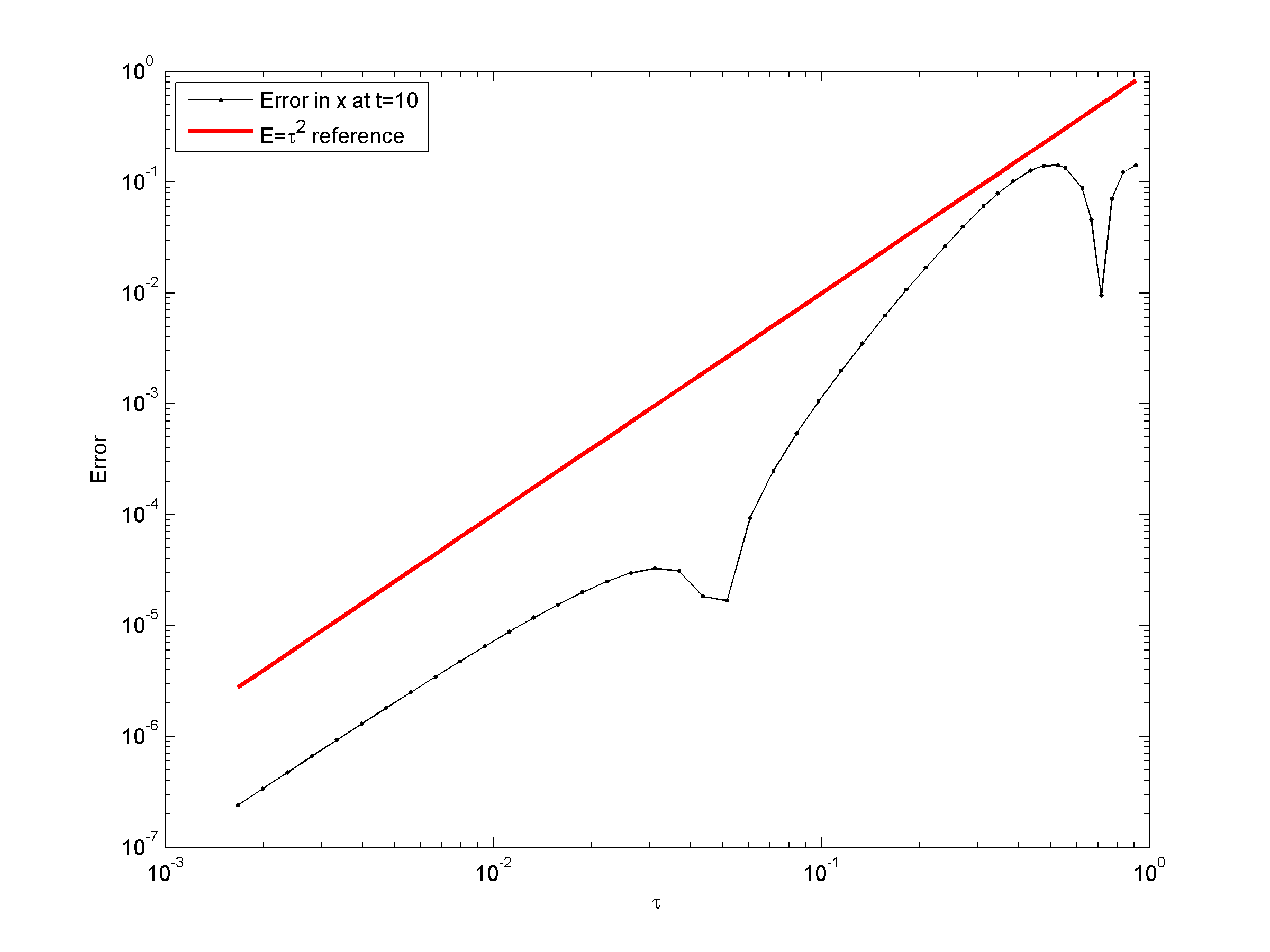
Indeed, it can be checked that the first term in (39) approaches m​xt​t+γ​xt+γ24​m​xmx_{tt}+\gamma x_{t}+\frac{\gamma^{2}}{4m}x as τ→0\tau\rightarrow 0 by l’Hôpital’s rule and the second term in (39) approaches (k−γ24​m)​x\left(k-\frac{\gamma^{2}}{4m}\right)x as τ→0\tau\rightarrow 0. In other words, FnτF^{\tau}_{n} defined in (39) is consistent with FF in (33), as claimed by Theorem 2. Moreover, since λτ\lambda^{\tau} in (37) and Dtτ​ψD_{t}^{\tau}\psi in (38) are second order accurate, FτF^{\tau} is second order accurate as well by Theorem 2. Multiplying (39) by (37) shows that the discrete density (36) is conserved for solutions of (39), as claimed by Theorem 3. In Appendix B, we include numerical verification of the order of accuracy and of the exact conservation for the discrete density ψτ\psi^{\tau} in (36).

4.3 Two body problem

Consider the ODE system of the two-body problem in 1D arising from classical physics,

𝑭⁡[𝒙]:=[xt​t1−V′​(x1−x2)xt​t2−V′​(x2−x1)]=𝟎,\boldsymbol{F}[\boldsymbol{x}]:=\begin{bmatrix}x^{1}_{tt}-V^{\prime}(x^{1}-x^{2})\\ x^{2}_{tt}-V^{\prime}(x^{2}-x^{1})\\ \end{bmatrix}=\boldsymbol{0},

where x1,x2x^{1},x^{2} are position of the two particles and VV is the interaction potential satisfying V′​(−z)=−V′​(z)V^{\prime}(-z)=-V^{\prime}(z). In this case, it’s known from Noether’s theorem that both momentum and energy is conserved. In particular, we have exactly two conservation laws

Dt​(xt1+xt2(xt1)2+(xt2)22+V⁡(x1−x2))|𝑭⁡[𝒙]=0=Λ⁡[𝒙]​𝑭​[𝒙]​|𝑭⁡[𝒙]=0=0,\left.D_{t}\begin{pmatrix}x^{1}_{t}+x^{2}_{t}\\ \frac{(x^{1}_{t})^{2}+(x^{2}_{t})^{2}}{2}+V(x^{1}-x^{2})\\ \end{pmatrix}\right|_{\boldsymbol{F}[\boldsymbol{x}]=0}=\left.\Lambda[\boldsymbol{x}]\boldsymbol{F}[\boldsymbol{x}]\frac{}{}\right|_{\boldsymbol{F}[\boldsymbol{x}]=0}=0,

and two sets of conservation law multipliers Λ\Lambda,

Λ⁡[𝒙]=(11xt1xt2),\Lambda[\boldsymbol{x}]=\begin{pmatrix}1&1\\ x^{1}_{t}&x^{2}_{t}\\ \end{pmatrix},

As in the previous two examples, we could have also found the multipliers and conservation laws through the method of Euler operator. We discretize 𝝍\boldsymbol{\psi} and Λ\Lambda by,

𝝍τ​{𝒙τ}n\displaystyle\boldsymbol{\psi}^{\tau}\{\boldsymbol{x}^{\tau}\}_{n} :=(xn+11−xn1τ+xn+12−xn2τ12​(xn+11−xn1τ)2+12​(xn+12−xn2τ)2+V⁡(xn+11−xn+12)+V⁡(xn1−xn2)2),\displaystyle:=\begin{pmatrix}\frac{x^{1}_{n+1}-x^{1}_{n}}{\tau}+\frac{x^{2}_{n+1}-x^{2}_{n}}{\tau}\\ \frac{1}{2}\left(\frac{x^{1}_{n+1}-x^{1}_{n}}{\tau}\right)^{2}+\frac{1}{2}\left(\frac{x^{2}_{n+1}-x^{2}_{n}}{\tau}\right)^{2}+\frac{V(x^{1}_{n+1}-x^{2}_{n+1})+V(x^{1}_{n}-x^{2}_{n})}{2}\\ \end{pmatrix}, (40)
Λτ​{𝒙τ}n\displaystyle\Lambda^{\tau}\{\boldsymbol{x}^{\tau}\}_{n} :=(11xn+11−xn−112​τxn+12−xn−122​τ).\displaystyle:=\begin{pmatrix}1&1\\ \frac{x^{1}_{n+1}-x^{1}_{n-1}}{2\tau}&\frac{x^{2}_{n+1}-x^{2}_{n-1}}{2\tau}\\ \end{pmatrix}. (41)

Then Dtτ​𝝍D_{t}^{\tau}\boldsymbol{\psi} given by (15a) simplifies to

Dtτ​𝝍​{𝒙τ}n\displaystyle D_{t}^{\tau}\boldsymbol{\psi}\{\boldsymbol{x}^{\tau}\}_{n} :=(xn+11−2​xn1+xn−11τ2+xn+12−2​xn2+xn−12τ2(xn+11−xn−11)​(xn+11−2​xn1+xn−11)2​τ3+(xn+12−xn−12)​(xn+12−2​xn2+xn−12)2​τ3+V⁡(xn+11−xn+12)−V⁡(xn−11−xn−12)2​τ).\displaystyle:=\begin{pmatrix}\frac{x^{1}_{n+1}-2x^{1}_{n}+x^{1}_{n-1}}{\tau^{2}}+\frac{x^{2}_{n+1}-2x^{2}_{n}+x^{2}_{n-1}}{\tau^{2}}\\ \frac{(x^{1}_{n+1}-x^{1}_{n-1})(x^{1}_{n+1}-2x^{1}_{n}+x^{1}_{n-1})}{2\tau^{3}}+\frac{(x^{2}_{n+1}-x^{2}_{n-1})(x^{2}_{n+1}-2x^{2}_{n}+x^{2}_{n-1})}{2\tau^{3}}+\frac{V(x^{1}_{n+1}-x^{2}_{n+1})-V(x^{1}_{n-1}-x^{2}_{n-1})}{2\tau}\\ \end{pmatrix}. (42)

Since Λτ,h\Lambda^{\tau,h} in (41) and Dtτ​𝝍D_{t}^{\tau}\boldsymbol{\psi} in (42) are both second order accurate, we have by Theorem 4 that the second order accurate discretization 𝑭τ\boldsymbol{F}^{\tau},

𝑭τ​{𝒙τ}n:=(xn+11−2​xn1+xn−11τ2+V⁡(xn+11−xn+12)−V⁡(xn−11−xn−12)xn+11−xn+12−xn−11+xn−12xn+12−2​xn2+xn−12τ2+V⁡(xn+12−xn+11)−V⁡(xn−12−xn−11)xn+12−xn+11−xn−12+xn−11)=𝟎.\boldsymbol{F}^{\tau}\{\boldsymbol{x}^{\tau}\}_{n}:=\begin{pmatrix}\frac{x^{1}_{n+1}-2x^{1}_{n}+x^{1}_{n-1}}{\tau^{2}}+\frac{V(x^{1}_{n+1}-x^{2}_{n+1})-V(x^{1}_{n-1}-x^{2}_{n-1})}{x^{1}_{n+1}-x^{2}_{n+1}-x^{1}_{n-1}+x^{2}_{n-1}}\\ \frac{x^{2}_{n+1}-2x^{2}_{n}+x^{2}_{n-1}}{\tau^{2}}+\frac{V(x^{2}_{n+1}-x^{1}_{n+1})-V(x^{2}_{n-1}-x^{1}_{n-1})}{x^{2}_{n+1}-x^{1}_{n+1}-x^{2}_{n-1}+x^{1}_{n-1}}\\ \end{pmatrix}=\boldsymbol{0}. (43)

Multiplying (43) by (41) shows that the discrete densities (40) are preserved.

4.4 Lotka-Volterra equations

Consider the Lotka-Volterra equations or the predator-prey equations,

𝑭⁡[𝒙]:=(xt−x⁡(a−b​y)yt+y⁡(c−d​x))=𝟎,\boldsymbol{F}[\boldsymbol{x}]:=\begin{pmatrix}x_{t}-x(a-by)\\ y_{t}+y(c-dx)\\ \end{pmatrix}=\boldsymbol{0},

where a,b,c,da,b,c,d are positive constants. It is known that this system has one conservation law,

Dt​(​log⁡(xc​ya)−d​x−b​y)|𝑭⁡[𝒙]=0=Λ⁡[𝒙]​𝑭​[𝒙]​|𝑭⁡[𝒙]=0=0,\left.D_{t}\left(\frac{}{}\log(x^{c}y^{a})-dx-by\right)\right|_{\boldsymbol{F}[\boldsymbol{x}]=0}=\left.\Lambda[\boldsymbol{x}]\boldsymbol{F}[\boldsymbol{x}]\frac{}{}\right|_{\boldsymbol{F}[\boldsymbol{x}]=0}=0,

with the 1×21\times 2 multiplier matrix Λ\Lambda,

Λ⁡[𝒙]=(cx−day−b).\Lambda[\boldsymbol{x}]=\begin{pmatrix}\frac{c}{x}-d&\frac{a}{y}-b\\ \end{pmatrix}. (44)

In particular, this system is of the kind where the number of conservation laws is less than the number of equations. Hence, we first partition (44) into 1×11\times 1 matrices Λ~\widetilde{\Lambda} and Σ\Sigma,

Λ~​[𝒙]=(cx−d),\displaystyle\widetilde{\Lambda}[\boldsymbol{x}]=\begin{pmatrix}\frac{c}{x}-d\end{pmatrix},
Σ⁡[𝒙]=(ay−b),\displaystyle\Sigma[\boldsymbol{x}]=\begin{pmatrix}\frac{a}{y}-b\end{pmatrix},

so that G⁡[𝒙]=yt+y⁡(c−d​x)G[\boldsymbol{x}]=y_{t}+y(c-dx). In order to use (22), we discretize ψ\psi, Λ~\widetilde{\Lambda}, Σ\Sigma, GG by

ψτ​{𝒙τ}n\displaystyle\psi^{\tau}\{\boldsymbol{x}^{\tau}\}_{n} :=log⁡(xnc​yna)−d​xn−b​yn,\displaystyle:=\log(x^{c}_{n}y^{a}_{n})-dx_{n}-by_{n}, (45)
Λ~τ​{𝒙τ}n\displaystyle\widetilde{\Lambda}^{\tau}\{\boldsymbol{x}^{\tau}\}_{n} :=(cxn−d),\displaystyle:=\begin{pmatrix}\frac{c}{x_{n}}-d\end{pmatrix},
Στ​{𝒙τ}n\displaystyle\Sigma^{\tau}\{\boldsymbol{x}^{\tau}\}_{n} :=(ayn−b),\displaystyle:=\begin{pmatrix}\frac{a}{y_{n}}-b\end{pmatrix},
Gτ​{𝒙τ}n\displaystyle G^{\tau}\{\boldsymbol{x}^{\tau}\}_{n} :=yn−yn−1τ+yn​(c−d​xn).\displaystyle:=\frac{y_{n}-y_{n-1}}{\tau}+y_{n}(c-dx_{n}).

Then Dtτ​ψD_{t}^{\tau}\psi defined by (26a) is,

Dtτ​ψ​{𝒙τ}n\displaystyle D_{t}^{\tau}\psi\{\boldsymbol{x}^{\tau}\}_{n} :=1τ​(log⁡(xnc​ynaxn−1c​yn−1a)−d⁡(xn−xn−1)−b⁡(yn−yn−1)).\displaystyle:=\frac{1}{\tau}\left(\log\left(\frac{x^{c}_{n}y^{a}_{n}}{x^{c}_{n-1}y^{a}_{n-1}}\right)-d(x_{n}-x_{n-1})-b(y_{n}-y_{n-1})\right).

Although Λ~τ\widetilde{\Lambda}^{\tau} and Σ~τ\widetilde{\Sigma}^{\tau} are exact discretization of Λ~\widetilde{\Lambda} and Σ~\widetilde{\Sigma}, Dtτ​ψD_{t}^{\tau}\psi and GτG^{\tau} are only first order accurate. So the discretization 𝑭τ{\boldsymbol{F}}^{\tau} given by (22) is at most first order by Theorem 6 and it simplifies to,

𝑭τ​{𝒙τ}n:=(1cxn−d​[c​log⁡xn−log⁡xn−1τ−d​xn−xn−1τ−(cxn−d)​xn​(a−b​yn)+a​log⁡yn−log⁡yn−1τ−ayn​yn−yn−1τ]yn−yn−1τ+yn​(c−d​xn))=𝟎.\boldsymbol{F}^{\tau}\{\boldsymbol{x}^{\tau}\}_{n}:=\begin{pmatrix}\frac{1}{\frac{c}{x_{n}}-d}\left[c\frac{\log x_{n}-\log x_{n-1}}{\tau}-d\frac{x_{n}-x_{n-1}}{\tau}-\left(\frac{c}{x_{n}}-d\right)x_{n}(a-by_{n})+a\frac{\log y_{n}-\log y_{n-1}}{\tau}-\frac{a}{y_{n}}\frac{y_{n}-y_{n-1}}{\tau}\right]\\ \frac{y_{n}-y_{n-1}}{\tau}+y_{n}(c-dx_{n})\end{pmatrix}=\boldsymbol{0}. (46)

It can be seen that by taking τ→0\tau\rightarrow 0, the first equation of 𝑭τ\boldsymbol{F}^{\tau} is consistent with the first equation of 𝑭\boldsymbol{F}. Moreover, it can be checked that solutions of (46) preserve (45).

4.5 Non-dissipative Lorenz equations

Consider the non-dissipative Lorenz equations,

𝑭⁡[𝒙]:=(xt−σ​yyt−x⁡(r−z)zt−x​y)=𝟎\boldsymbol{F}[\boldsymbol{x}]:=\begin{pmatrix}x_{t}-\sigma y\\ y_{t}-x(r-z)\\ z_{t}-xy\end{pmatrix}=\boldsymbol{0}

where σ,r\sigma,r are positive constants. It was found in [NB94] that this system has 22 conservation laws,

Dt​(z−x22​σy22+z22−r​z)|𝑭⁡[𝒙]=0=Λ⁡[𝒙]​𝑭​[𝒙]​|𝑭⁡[𝒙]=0=0,\left.D_{t}\begin{pmatrix}z-\frac{x^{2}}{2\sigma}\\ \frac{y^{2}}{2}+\frac{z^{2}}{2}-rz\\ \end{pmatrix}\right|_{\boldsymbol{F}[\boldsymbol{x}]=0}=\left.\Lambda[\boldsymbol{x}]\boldsymbol{F}[\boldsymbol{x}]\frac{}{}\right|_{\boldsymbol{F}[\boldsymbol{x}]=0}=0,

with the 2×32\times 3 multiplier matrix Λ\Lambda,

Λ⁡[𝒙]=(−xσ010yz−r).\Lambda[\boldsymbol{x}]=\begin{pmatrix}-\frac{x}{\sigma}&0&1\\ 0&y&z-r\\ \end{pmatrix}. (47)

Similar to the previous example, we partition (47) into 2×22\times 2 matrix Λ~\widetilde{\Lambda} and 1×21\times 2 matrix Σ\Sigma,

Λ~​[𝒙]=(−xσ00y),\displaystyle\widetilde{\Lambda}[\boldsymbol{x}]=\begin{pmatrix}-\frac{x}{\sigma}&0\\ 0&y\end{pmatrix},
Σ⁡[𝒙]=(1z−r),\displaystyle\Sigma[\boldsymbol{x}]=\begin{pmatrix}1\\ z-r\end{pmatrix},

with G⁡[𝒙]=zt−x​yG[\boldsymbol{x}]=z_{t}-xy. To simplify the final discretization as much as possible, we choose the following discretization ψ\psi, Λ~\widetilde{\Lambda}, Σ\Sigma, GG by

𝝍τ​{𝒙τ}n\displaystyle\boldsymbol{\psi}^{\tau}\{\boldsymbol{x}^{\tau}\}_{n} :=(zn−xn22​σyn22+zn22−r​zn),\displaystyle:=\begin{pmatrix}z_{n}-\frac{x_{n}^{2}}{2\sigma}\\ \frac{y_{n}^{2}}{2}+\frac{z_{n}^{2}}{2}-rz_{n}\end{pmatrix}, (48)
Λ~τ​{𝒙τ}n\displaystyle\widetilde{\Lambda}^{\tau}\{\boldsymbol{x}^{\tau}\}_{n} :=(−xn+xn−12​σ00yn+yn−12),\displaystyle:=\begin{pmatrix}-\frac{x_{n}+x_{n-1}}{2\sigma}&0\\ 0&\frac{y_{n}+y_{n-1}}{2}\end{pmatrix}, (49)
Στ​{𝒙τ}n\displaystyle\Sigma^{\tau}\{\boldsymbol{x}^{\tau}\}_{n} :=(1zn+zn−12−r),\displaystyle:=\begin{pmatrix}1\\ \frac{z_{n}+z_{n-1}}{2}-r\end{pmatrix}, (50)
Gτ​{𝒙τ}n\displaystyle G^{\tau}\{\boldsymbol{x}^{\tau}\}_{n} :=zn−zn−1τ−xn+xn−12​yn+yn−12.\displaystyle:=\frac{z_{n}-z_{n-1}}{\tau}-\frac{x_{n}+x_{n-1}}{2}\frac{y_{n}+y_{n-1}}{2}.

Then Dtτ​ψD_{t}^{\tau}\psi defined by (26a) is,

Dtτ​𝝍​{𝒙τ}n\displaystyle D_{t}^{\tau}\boldsymbol{\psi}\{\boldsymbol{x}^{\tau}\}_{n} :=(zn−zn−1τ−xn2−xn−122​σ​τyn2−yn−122​τ+zn2−zn−122​τ−r​zn−zn−1τ).\displaystyle:=\begin{pmatrix}\frac{z_{n}-z_{n-1}}{\tau}-\frac{x_{n}^{2}-x_{n-1}^{2}}{2\sigma\tau}\\ \frac{y_{n}^{2}-y_{n-1}^{2}}{2\tau}+\frac{z_{n}^{2}-z_{n-1}^{2}}{2\tau}-r\frac{z_{n}-z_{n-1}}{\tau}\end{pmatrix}.

Since Λ~τ\widetilde{\Lambda}^{\tau} and Σ~τ\widetilde{\Sigma}^{\tau} are second order accurate and Dtτ​ψD_{t}^{\tau}\psi and GτG^{\tau} are only first order accurate, we expect the discretization to be at most first order by Theorem 6. Using (22), the discretization 𝑭τ{\boldsymbol{F}}^{\tau} simplifies to,

𝑭τ​{𝒙τ}n:=(xn−xn−1τ−σ​yn+yn−12yn−yn−1τ−xn+xn−12​(r−zn+zn−12)zn−zn−1τ−xn+xn−12​yn+yn−12)=𝟎.\boldsymbol{F}^{\tau}\{\boldsymbol{x}^{\tau}\}_{n}:=\begin{pmatrix}\frac{x_{n}-x_{n-1}}{\tau}-\sigma\frac{y_{n}+y_{n-1}}{2}\\ \frac{y_{n}-y_{n-1}}{\tau}-\frac{x_{n}+x_{n-1}}{2}(r-\frac{z_{n}+z_{n-1}}{2})\\ \frac{z_{n}-z_{n-1}}{\tau}-\frac{x_{n}+x_{n-1}}{2}\frac{y_{n}+y_{n-1}}{2}\end{pmatrix}=\boldsymbol{0}. (51)

Multiplying (51) by the discrete multiplier Λτ=(Λ~τ​Στ)\Lambda^{\tau}=\left(\widetilde{\Lambda}^{\tau}\hskip 5.69054pt\Sigma^{\tau}\right) defined by (49), (50) shows the discrete densities (48) are preserved.

4.6 Inviscid Burgers’ equation

Next we illustrate this method for the inviscid Burgers’ equation,

F⁡[u]:=ut+u​ux=0.F[u]:=u_{t}+uu_{x}=0. (52)

Writing (52) in conserved form, it is well-known that it has the conservation law,

(Dt​u+Dx​(u22))|F⁡[u]=0=λ⁡[u]⋅F⁡[u]​|F⁡[u]=0=0,\left.\left(D_{t}u+D_{x}\left(\frac{u^{2}}{2}\right)\right)\right|_{F[u]=0}=\left.\lambda[u]\cdot F[u]\frac{}{}\right|_{F[u]=0}=0,

which corresponds to a multiplier of λ⁡[u]=1\lambda[u]=1. Now suppose we discretize ψ\psi, ϕ\phi, λ\lambda with the following expressions,

ψτ,h​{uτ,h}n,j\displaystyle\psi^{\tau,h}\{u^{\tau,h}\}_{n,j} :=un,j,\displaystyle:=u_{n,j},
ϕτ,h​{uτ,h}n,j\displaystyle\phi^{\tau,h}\{u^{\tau,h}\}_{n,j} :=un,j22,\displaystyle:=\frac{u_{n,j}^{2}}{2}, (53)
λτ,h​{uτ,h}n,j\displaystyle\lambda^{\tau,h}\{u^{\tau,h}\}_{n,j} :=1.\displaystyle:=1.

Then, Dtτ,h​ψD_{t}^{\tau,h}\psi, Dxτ,h​ϕD_{x}^{\tau,h}\phi defined by (6a), (6b) are,

Dtτ,h​ψ​{uτ,h}n,j\displaystyle D_{t}^{\tau,h}\psi\{u^{\tau,h}\}_{n,j} :=un,j−un−1,jτ,\displaystyle:=\frac{u_{n,j}-u_{n-1,j}}{\tau},
Dxτ,h​ϕ​{uτ,h}n,j\displaystyle D_{x}^{\tau,h}\phi\{u^{\tau,h}\}_{n,j} :=(un,j)2−(un,j−1)22​h.\displaystyle:=\frac{(u_{n,j})^{2}-(u_{n,j-1})^{2}}{2h}.

So by (3), we obtain the well-known conservative discretization of (52) which preserves (53),

Fτ,h​{uτ,h}n,j:=un,j−un−1,jτ+(un,j)2−(un,j−1)22​h=0,F^{\tau,h}\{u^{\tau,h}\}_{n,j}:=\frac{u_{n,j}-u_{n-1,j}}{\tau}+\frac{(u_{n,j})^{2}-(u_{n,j-1})^{2}}{2h}=0, (54)

which is clearly first order in time and in space.

To make this example more interesting, let us consider other conservation laws of (52). By the method of Euler operator (or inspired guess), the inviscid Burgers’ equation has a family of conservation law multiplier λ⁡[u]=up−1\lambda[u]=u^{p-1} for p∈ℕp\in\mathbb{N} with the conservation law,

(Dt​(upp)+Dx​(up+1p+1))|F⁡[u]=0=λ⁡[u]⋅F⁡[u]​|F⁡[u]=0=0.\left.\left(D_{t}\left(\frac{u^{p}}{p}\right)+D_{x}\left(\frac{u^{p+1}}{p+1}\right)\right)\right|_{F[u]=0}=\left.\lambda[u]\cdot F[u]\frac{}{}\right|_{F[u]=0}=0.

Similar to before, we discretize ψ\psi, ϕ\phi , λ\lambda with the expressions,

ψτ,h​{uτ,h}n,j\displaystyle\psi^{\tau,h}\{u^{\tau,h}\}_{n,j} :=(un,j)pp,\displaystyle:=\frac{(u_{n,j})^{p}}{p}, (55)
ϕτ,h​{uτ,h}n,j\displaystyle\phi^{\tau,h}\{u^{\tau,h}\}_{n,j} :=un,jp+1p+1,\displaystyle:=\frac{u_{n,j}^{p+1}}{p+1}, (56)
λτ,h​{uτ,h}n,j\displaystyle\lambda^{\tau,h}\{u^{\tau,h}\}_{n,j} :=1p​∑k=0p−1(un,j)p−1−k​(un−1,j)k.\displaystyle:=\frac{1}{p}\sum_{k=0}^{p-1}(u_{n,j})^{p-1-k}(u_{n-1,j})^{k}. (57)

It turns out the choice for the time averaged expression (57) of λn,jτ,h\lambda^{\tau,h}_{n,j} simplifies the final expression of the discretization. Similar as before, Dtτ,h​ψD_{t}^{\tau,h}\psi, Dxτ,h​ϕD_{x}^{\tau,h}\phi defined by (6a), (6b) are,

Dtτ,h​ψ​{uτ,h}n,j\displaystyle D_{t}^{\tau,h}\psi\{u^{\tau,h}\}_{n,j} :=(un,j)p−(un−1,j)pp​τ,\displaystyle:=\frac{(u_{n,j})^{p}-(u_{n-1,j})^{p}}{p\tau}, (58a)
Dxτ,h​ϕ​{uτ,h}n,j\displaystyle D_{x}^{\tau,h}\phi\{u^{\tau,h}\}_{n,j} :=(un,j)p+1−(un,j−1)p+1(p+1)​h,\displaystyle:=\frac{(u_{n,j})^{p+1}-(u_{n,j-1})^{p+1}}{(p+1)h}, (58b)

It can be shown that λτ,h\lambda^{\tau,h} in (55) and Dtτ,h​ψD_{t}^{\tau,h}\psi in (58a) are first order accurate in time and Dxτ,h​ϕD_{x}^{\tau,h}\phi is first order accurate in space. By Theorem 2, the discretization of (3) is first order in space and time. Employing the identity, ap+1−bp+1=(a−b)​∑k=0pap−k​bk\displaystyle a^{p+1}-b^{p+1}=(a-b)\sum_{k=0}^{p}a^{p-k}b^{k}, Fτ,hF^{\tau,h} simplifies to,

Fτ,h​{uτ,h}n,j\displaystyle F^{\tau,h}\{u^{\tau,h}\}_{n,j} :=un,j−un−1,jτ\displaystyle:=\frac{u_{n,j}-u_{n-1,j}}{\tau}
+pp+1​(un,j)p+(un,j)p−1​un,j−1+⋯+un,j​(un,j−1)p−1+(un,j−1)p(un,j)p−1+(un,j)p−2​un−1,j+⋯+un,j​(un−1,j)p−2+(un−1,j)p−1​un,j−un,j−1h=0,\displaystyle\hskip 17.07164pt+\frac{p}{p+1}\frac{(u_{n,j})^{p}+(u_{n,j})^{p-1}u_{n,j-1}+\cdots+u_{n,j}(u_{n,j-1})^{p-1}+(u_{n,j-1})^{p}}{(u_{n,j})^{p-1}+(u_{n,j})^{p-2}u_{n-1,j}+\cdots+u_{n,j}(u_{n-1,j})^{p-2}+(u_{n-1,j})^{p-1}}\frac{u_{n,j}-u_{n,j-1}}{h}=0, (59)

which can readily be checked to preserve the discrete density (55) when the fluxes (56) vanish at the boundaries. Moreover, (59) can be seen as a generalization to (54), with p=1p=1.

4.7 Korteweg-de Vries equation

Next we consider the Korteweg-de Vries equation,

F⁡[u]:=ut+u​ux+ux​x​x=0.F[u]:=u_{t}+uu_{x}+u_{xxx}=0. (60)

As written, (60) does not admit a variational principle. Indeed, it is well known that upon the change of variable u=vxu=v_{x}, (60) is the Euler-Lagrange equations of a Lagrangian. Our main motivation here is to show that we can construct a conservative discretization of the Korteweg-de Vries equation without such transformation.

It can be checked (or by the method of Euler operator) that (60) has a multiplier λ⁡[u]=u\lambda[u]=u with the corresponding density and flux,

(Dt​(u22)+Dx​(u33+u​ux​x−ux22))|F⁡[u]=0=λ⁡[u]⋅F⁡[u]​|F⁡[u]=0=0.\left.\left(D_{t}\left(\frac{u^{2}}{2}\right)+D_{x}\left(\frac{u^{3}}{3}+uu_{xx}-\frac{u_{x}^{2}}{2}\right)\right)\right|_{F[u]=0}=\left.\lambda[u]\cdot F[u]\frac{}{}\right|_{F[u]=0}=0.

To simplify the final expression for Fτ,hF^{\tau,h}, we choose to discretize ψ,ϕ,λ\psi,\phi,\lambda as follows,

ψτ,h​{uτ,h}n,j\displaystyle\psi^{\tau,h}\{u^{\tau,h}\}_{n,j} :=un,j22,\displaystyle:=\frac{u_{n,j}^{2}}{2}, (61)
ϕτ,h​{uτ,h}n,j\displaystyle\phi^{\tau,h}\{u^{\tau,h}\}_{n,j} :=un,j33+(un,j+1+un,j2)​(un,j+1−2​un,j+un,j−1h2)−12​(un,j+1−un,jh)2,\displaystyle:=\frac{u_{n,j}^{3}}{3}+\left(\frac{u_{n,j+1}+u_{n,j}}{2}\right)\left(\frac{u_{n,j+1}-2u_{n,j}+u_{n,j-1}}{h^{2}}\right)-\frac{1}{2}\left(\frac{u_{n,j+1}-u_{n,j}}{h}\right)^{2}, (62)
λτ,h​{uτ,h}n,j\displaystyle\lambda^{\tau,h}\{u^{\tau,h}\}_{n,j} :=un,j+un−1,j2.\displaystyle:=\frac{u_{n,j}+u_{n-1,j}}{2}. (63)

Thus, (6a) and (6b) simplify to

Dtτ,h​ψ​{uτ,h}n,j\displaystyle D_{t}^{\tau,h}\psi\{u^{\tau,h}\}_{n,j} :=(un,j)2−(un−1,j)22​τ,\displaystyle:=\frac{(u_{n,j})^{2}-(u_{n-1,j})^{2}}{2\tau}, (64)
Dxτ,h​ϕ​{uτ,h}n,j\displaystyle D_{x}^{\tau,h}\phi\{u^{\tau,h}\}_{n,j} :=(un,j)3−(un,j−1)33​h+(un,j+un,j−12)​(un,j+1−3​un,j+3​un,j−1−un,j−2h3).\displaystyle:=\frac{(u_{n,j})^{3}-(u_{n,j-1})^{3}}{3h}+\left(\frac{u_{n,j}+u_{n,j-1}}{2}\right)\left(\frac{u_{n,j+1}-3u_{n,j}+3u_{n,j-1}-u_{n,j-2}}{h^{3}}\right). (65)

One can see that λτ,h\lambda^{\tau,h} in (63) and Dtτ,h​ψD_{t}^{\tau,h}\psi in (64) are first order accurate in time and Dxτ,h​ϕD_{x}^{\tau,h}\phi in (65) is first order in space. Thus, it follows from Theorem 2 that,

Fτ,h​{uτ,h}n,j:=un,j−un−1,jτ\displaystyle F^{\tau,h}\{u^{\tau,h}\}_{n,j}:=\frac{u_{n,j}-u_{n-1,j}}{\tau} +2​(un,j2+un,j​un,j−1+un,j−12)3​(un,j+un−1,j)​(un,j−un,j−1h)\displaystyle+\frac{2(u_{n,j}^{2}+u_{n,j}u_{n,j-1}+u_{n,j-1}^{2})}{3(u_{n,j}+u_{n-1,j})}\left(\frac{u_{n,j}-u_{n,j-1}}{h}\right)
+(un,j+un,j−1un,j+un−1,j)​(un,j+1−3​un,j+3​un,j−1−un,j−2h3)=0,\displaystyle+\left(\frac{u_{n,j}+u_{n,j-1}}{u_{n,j}+u_{n-1,j}}\right)\left(\frac{u_{n,j+1}-3u_{n,j}+3u_{n,j-1}-u_{n,j-2}}{h^{3}}\right)=0,

is a first order discretization of (60) that preserves the discrete density (61) when the fluxes (62) vanish at the boundary.

4.8 Shallow water PDE system

Lastly, we consider the two-dimensional shallow-water equations in non-dimensional form

𝑭⁡[𝒖]:=(ut+𝐯⋅∇u+ηxvt+𝐯⋅∇v+ηyηt+∇⋅(η​𝐯))=𝟎,\displaystyle\boldsymbol{F}[\boldsymbol{u}]:=\begin{pmatrix}u_{t}+\mathbf{v}\cdot\nabla u+\eta_{x}\\ v_{t}+\mathbf{v}\cdot\nabla v+\eta_{y}\\ \eta_{t}+\nabla\cdot(\eta\mathbf{v})\end{pmatrix}=\boldsymbol{0}, (66)

where 𝐯=(u,v)\mathbf{v}=(u,v) is the two-dimensional velocity field and η\eta is the displacement of the water surface over a constant reference level. It is well-known that this system admits conservation of momentum and mass. The multiplier form of these conservation laws is

(Dt​(η​uη​vη)+Dx​(η​u2+12​η2η​u​vη​u)+Dy​(η​u​vη​v2+12​η2η​v))|𝑭⁡[𝒖]=0\displaystyle\left.\left(D_{t}\begin{pmatrix}\eta u\\ \eta v\\ \eta\end{pmatrix}+D_{x}\begin{pmatrix}\eta u^{2}+\frac{1}{2}\eta^{2}\\ \eta uv\\ \eta u\end{pmatrix}+D_{y}\begin{pmatrix}\eta uv\\ \eta v^{2}+\frac{1}{2}\eta^{2}\\ \eta v\end{pmatrix}\right)\right|_{\boldsymbol{F}[\boldsymbol{u}]=0} =(η0u0ηv001)​(ut+𝐯⋅∇u+ηxvt+𝐯⋅∇v+ηyηt+∇⋅(η​𝐯))|𝑭⁡[𝒖]=0\displaystyle=\left(\begin{array}[]{ccc}\eta&0&u\\ 0&\eta&v\\ 0&0&1\end{array}\right)\left.\left(\begin{array}[]{c}u_{t}+\mathbf{v}\cdot\nabla u+\eta_{x}\\ v_{t}+\mathbf{v}\cdot\nabla v+\eta_{y}\\ \eta_{t}+\nabla\cdot(\eta\mathbf{v})\end{array}\right)\right|_{\boldsymbol{F}[\boldsymbol{u}]=0}
=𝟎.\displaystyle={\boldsymbol{0}}.

Choosing the discretization for 𝝍\boldsymbol{\psi}, ϕ\boldsymbol{\phi} and Λ\Lambda,

𝝍τ,h​{𝒖τ,h}n,i,j\displaystyle\boldsymbol{\psi}^{\tau,h}\{\boldsymbol{u}^{\tau,h}\}_{n,i,j} =(ηn,i,j​un,i,jηn,i,j​vn,i,jηn,i,j),\displaystyle=\begin{pmatrix}\eta_{n,i,j}u_{n,i,j}\\ \eta_{n,i,j}v_{n,i,j}\\ \eta_{n,i,j}\end{pmatrix},
𝚽τ,h​{𝒖τ,h}n,i,j\displaystyle\boldsymbol{\Phi}^{\tau,h}\{\boldsymbol{u}^{\tau,h}\}_{n,i,j} =(ηn,i,j​un,i,j2+12​ηn,i,j2ηn,i,j​un,i,j​vn,i,jηn,i,j​un,i,j​vn,i,jηn,i,j​vn,i,j2+12​ηn,i,j2ηn,i,j​un,i,jηn,i,j​vn,i,j),\displaystyle=\begin{pmatrix}\eta_{n,i,j}u_{n,i,j}^{2}+\frac{1}{2}\eta_{n,i,j}^{2}&\eta_{n,i,j}u_{n,i,j}v_{n,i,j}\\ \eta_{n,i,j}u_{n,i,j}v_{n,i,j}&\eta_{n,i,j}v_{n,i,j}^{2}+\frac{1}{2}\eta_{n,i,j}^{2}\\ \eta_{n,i,j}u_{n,i,j}&\eta_{n,i,j}v_{n,i,j}\end{pmatrix},
Λτ,h​{𝒖τ,h}n,i,j\displaystyle\Lambda^{\tau,h}\{\boldsymbol{u}^{\tau,h}\}_{n,i,j} =(ηn,i,j+ηn−1,i,j20un,i,j+un−1,i,j20ηn,i,j+ηn−1,i,j2vn,i,j+vn−1,i,j2001),\displaystyle=\begin{pmatrix}\frac{\eta_{n,i,j}+\eta_{n-1,i,j}}{2}&0&\frac{u_{n,i,j}+u_{n-1,i,j}}{2}\\ 0&\frac{\eta_{n,i,j}+\eta_{n-1,i,j}}{2}&\frac{v_{n,i,j}+v_{n-1,i,j}}{2}\\ 0&0&1\end{pmatrix}, (67)

then Dtτ,h​𝝍D_{t}^{\tau,h}\boldsymbol{\psi} and Dtτ,h​ϕD_{t}^{\tau,h}\boldsymbol{\phi} defined by (26a) and (26b) are

Dtτ,h​𝝍​{𝒖τ,h}n,i,j\displaystyle D_{t}^{\tau,h}\boldsymbol{\psi}\{\boldsymbol{u}^{\tau,h}\}_{n,i,j} :=(ηn,i,j​un,i,j−ηn−1,i,j​un−1,i,jτηn,i,j​vn,i,j−ηn−1,i,j​vn−1,i,jτηn,i,j−ηn−1,i,jτ),\displaystyle:=\begin{pmatrix}\frac{\eta_{n,i,j}u_{n,i,j}-\eta_{n-1,i,j}u_{n-1,i,j}}{\tau}\\ \frac{\eta_{n,i,j}v_{n,i,j}-\eta_{n-1,i,j}v_{n-1,i,j}}{\tau}\\ \frac{\eta_{n,i,j}-\eta_{n-1,i,j}}{\tau}\end{pmatrix}, (68)
D𝒙τ,h⋅𝚽​{𝒖τ,h}n,i,j\displaystyle D_{\boldsymbol{x}}^{\tau,h}\cdot\boldsymbol{\Phi}\{\boldsymbol{u}^{\tau,h}\}_{n,i,j} :=(ηn,i,j​un,i,j2−ηn,i−1,j​un,i−1,j2h+12​ηn,i,j2−ηn,i−1,j2h+ηn,i,j​un,i,j​vn,i,j−ηn,i,j−1​un,i,j−1​vn,i,j−1hηn,i,j​un,i,j​vn,i,j−ηn,i+1,j​un,i+1,j​vn,i+1,jh+ηn,i,j​vn,i,j2−ηn,i,j−1​vn,i,j−12h+12​ηn,i,j2−ηn,i,j−12hηn,i,j​un,i,j−ηn,i−1,j​un,i−1,jh+ηn,i,j​vn,i,j−ηn,i,j−1​vn,i,j−1h).\displaystyle:=\begin{pmatrix}\frac{\eta_{n,i,j}u_{n,i,j}^{2}-\eta_{n,i-1,j}u_{n,i-1,j}^{2}}{h}+\frac{1}{2}\frac{\eta_{n,i,j}^{2}-\eta_{n,i-1,j}^{2}}{h}+\frac{\eta_{n,i,j}u_{n,i,j}v_{n,i,j}-\eta_{n,i,j-1}u_{n,i,j-1}v_{n,i,j-1}}{h}\\ \frac{\eta_{n,i,j}u_{n,i,j}v_{n,i,j}-\eta_{n,i+1,j}u_{n,i+1,j}v_{n,i+1,j}}{h}+\frac{\eta_{n,i,j}v_{n,i,j}^{2}-\eta_{n,i,j-1}v_{n,i,j-1}^{2}}{h}+\frac{1}{2}\frac{\eta_{n,i,j}^{2}-\eta_{n,i,j-1}^{2}}{h}\\ \frac{\eta_{n,i,j}u_{n,i,j}-\eta_{n,i-1,j}u_{n,i-1,j}}{h}+\frac{\eta_{n,i,j}v_{n,i,j}-\eta_{n,i,j-1}v_{n,i,j-1}}{h}\end{pmatrix}. (69)

Using (12), the entries of the discretization 𝑭τ,h{\boldsymbol{F}}^{\tau,h} simplifies to,

(𝑭τ,h​{𝒖τ,h}n,i,j)1\displaystyle\left(\boldsymbol{F}^{\tau,h}\{\boldsymbol{u}^{\tau,h}\}_{n,i,j}\right)_{1}
=un,i,j−un−1,i,jτ+(2​ηn,i−1,jηn,i,j+ηn−1,i,j)​(un,i,j+un,i−1,j−un,i,j+un−1,i,j2)​(un,i,j−un,i−1,jh)\displaystyle\qquad=\frac{u_{n,i,j}-u_{n-1,i,j}}{\tau}+\left(\frac{2\eta_{n,i-1,j}}{\eta_{n,i,j}+\eta_{n-1,i,j}}\right)\left(u_{n,i,j}+u_{n,i-1,j}-\frac{u_{n,i,j}+u_{n-1,i,j}}{2}\right)\left(\frac{u_{n,i,j}-u_{n,i-1,j}}{h}\right)
+(2​ηn,i,jηn,i,j+ηn−1,i,j)​vn,i,j​(un,i,j−un,i,j−1h)+(ηn,i,j+ηn,i−1,jηn,i,j+ηn−1,i,j)​(ηn,i,j−ηn,i−1,jh)\displaystyle\qquad+\left(\frac{2\eta_{n,i,j}}{\eta_{n,i,j}+\eta_{n-1,i,j}}\right)v_{n,i,j}\left(\frac{u_{n,i,j}-u_{n,i,j-1}}{h}\right)+\left(\frac{\eta_{n,i,j}+\eta_{n,i-1,j}}{\eta_{n,i,j}+\eta_{n-1,i,j}}\right)\left(\frac{\eta_{n,i,j}-\eta_{n,i-1,j}}{h}\right)
+(2ηn,i,j+ηn−1,i,j)​(ηn,i,j−ηn,i−1,jh)​un,i,j​(un,i,j−un,i,j+un−1,i,j2)\displaystyle\qquad+\left(\frac{2}{\eta_{n,i,j}+\eta_{n-1,i,j}}\right)\left(\frac{\eta_{n,i,j}-\eta_{n,i-1,j}}{h}\right)u_{n,i,j}\left(u_{n,i,j}-\frac{u_{n,i,j}+u_{n-1,i,j}}{2}\right)
(2ηn,i,j+ηn−1,i,j)​(ηn,i,j​vn,i,j−ηn,i,j−1​vn,i,j−1h)​(un,i,j−1−un,i,j+un−1,i,j2),\displaystyle\qquad\left(\frac{2}{\eta_{n,i,j}+\eta_{n-1,i,j}}\right)\left(\frac{\eta_{n,i,j}v_{n,i,j}-\eta_{n,i,j-1}v_{n,i,j-1}}{h}\right)\left(u_{n,i,j-1}-\frac{u_{n,i,j}+u_{n-1,i,j}}{2}\right), (70)
(𝑭τ,h​{𝒖τ,h}n,i,j)2\displaystyle\left(\boldsymbol{F}^{\tau,h}\{\boldsymbol{u}^{\tau,h}\}_{n,i,j}\right)_{2}
=vn,i,j−vn−1,i,jτ+(2​ηn,i,j−1ηn,i,j+ηn−1,i,j)​(vn,i,j+vn,i,j−1−vn,i,j+vn−1,i,j2)​(vn,i,j−vn,i,j−1h)\displaystyle\qquad=\frac{v_{n,i,j}-v_{n-1,i,j}}{\tau}+\left(\frac{2\eta_{n,i,j-1}}{\eta_{n,i,j}+\eta_{n-1,i,j}}\right)\left(v_{n,i,j}+v_{n,i,j-1}-\frac{v_{n,i,j}+v_{n-1,i,j}}{2}\right)\left(\frac{v_{n,i,j}-v_{n,i,j-1}}{h}\right)
+(2​ηn,i,jηn,i,j+ηn−1,i,j)​un,i,j​(vn,i,j−vn,i−1,jh)+(ηn,i,j+ηn,i,j−1ηn,i,j+ηn−1,i,j)​(ηn,i,j−ηn,i,j−1h)\displaystyle\qquad+\left(\frac{2\eta_{n,i,j}}{\eta_{n,i,j}+\eta_{n-1,i,j}}\right)u_{n,i,j}\left(\frac{v_{n,i,j}-v_{n,i-1,j}}{h}\right)+\left(\frac{\eta_{n,i,j}+\eta_{n,i,j-1}}{\eta_{n,i,j}+\eta_{n-1,i,j}}\right)\left(\frac{\eta_{n,i,j}-\eta_{n,i,j-1}}{h}\right)
+(2ηn,i,j+ηn−1,i,j)​(ηn,i,j−ηn,i,j−1h)​vn,i,j​(vn,i,j−vn,i,j+vn−1,i,j2)\displaystyle\qquad+\left(\frac{2}{\eta_{n,i,j}+\eta_{n-1,i,j}}\right)\left(\frac{\eta_{n,i,j}-\eta_{n,i,j-1}}{h}\right)v_{n,i,j}\left(v_{n,i,j}-\frac{v_{n,i,j}+v_{n-1,i,j}}{2}\right)
(2ηn,i,j+ηn−1,i,j)​(ηn,i,j​un,i,j−ηn,i−1,j​un,i−1,jh)​(vn,i−1,j−vn,i,j+vn−1,i,j2),\displaystyle\qquad\left(\frac{2}{\eta_{n,i,j}+\eta_{n-1,i,j}}\right)\left(\frac{\eta_{n,i,j}u_{n,i,j}-\eta_{n,i-1,j}u_{n,i-1,j}}{h}\right)\left(v_{n,i-1,j}-\frac{v_{n,i,j}+v_{n-1,i,j}}{2}\right), (71)
(𝑭τ,h​{𝒖τ,h}n,i,j)3=ηn,i,j−ηn−1,i,jτ+ηn,i,j​un,i,j−ηn,i−1,j​un,i−1,jh+ηn,i,j​vn,i,j−ηn,i,j−1​vn,i,j−1h.\displaystyle\left(\boldsymbol{F}^{\tau,h}\{\boldsymbol{u}^{\tau,h}\}_{n,i,j}\right)_{3}=\frac{\eta_{n,i,j}-\eta_{n-1,i,j}}{\tau}+\frac{\eta_{n,i,j}u_{n,i,j}-\eta_{n,i-1,j}u_{n,i-1,j}}{h}+\frac{\eta_{n,i,j}v_{n,i,j}-\eta_{n,i,j-1}v_{n,i,j-1}}{h}. (72)

Note that, as h→0h\rightarrow 0, the first four terms of (70) and (71) approaches the limit ut+u​ux+v​uy+ηxu_{t}+uu_{x}+vu_{y}+\eta_{x} and vt+v​vy+u​vx+ηyv_{t}+vv_{y}+uv_{x}+\eta_{y}, respectively. Also, the last two terms in (70) and (71) vanish, as expected in order for (70)-(72) to be consistent with (66). In particular, it can be seen that Λτ,h\Lambda^{\tau,h} in (67) and Dtτ,h​𝝍D_{t}^{\tau,h}\boldsymbol{\psi} in (68) are first order in time and D𝒙τ,h⋅𝚽D_{\boldsymbol{x}}^{\tau,h}\cdot\boldsymbol{\Phi} in (69) is first order in space. Thus, the proposed discretization 𝑭τ,h{\boldsymbol{F}}^{\tau,h} is first order accurate by Theorem 4.

5 Consistency when the inverse of the discrete multiplier is singular

In Sections 3.1, 3.2 and 3.3, consistencies of the multiplier method were shown provided that the inverse of the discrete multiplier Λτ,h\Lambda^{\tau,h} do not become singular on the mesh points in ℐτ×Ωh\mathcal{I}^{\tau}\times\Omega^{h}. In general, this may not be satisfied depending on the nature of the discrete solution 𝒖τ,h\boldsymbol{u}^{\tau,h}. We now provide a partial answer for establishing consistency in the case for scalar ODEs when the inverse of the discrete multiplier become singular. We comment on the generalization to system of ODEs in the conclusion.

5.1 Zero-compatibility condition and consistency for scalar ODEs

The main idea is as follows: Rather than arbitrary choices of discrete multiplier λτ​{uτ}\lambda^{\tau}\{u^{\tau}\} and discrete density Dtτ​ψ​{uτ}D_{t}^{\tau}\psi\{u^{\tau}\}, the pair should be chosen in a “compatible” manner which mimics the zero properties of λ⁡[u]\lambda[u] and Dt​ψ​[u]D_{t}\psi[u]. In particular, if λ⁡[u]\lambda[u] is a conservation law multiplier of F⁡[u]F[u] with density ψ⁡[u]\psi[u], then for any uu such that,

λ​[u]ti=0⇒λ​[u]ti​F​[u]ti=Dt​ψ​[u]ti=0.\lambda[u]_{t_{i}}=0\Rightarrow\lambda[u]_{t_{i}}F[u]_{t_{i}}=D_{t}\psi[u]_{t_{i}}=0. (73)

The discrete analog of (73) leads to the zero-compatibility condition of the multiplier method for scalar ODEs. For clarity, we shall assume μ\mu-step finite difference approximations for the discrete multiplier λτ​{uτ}i=λτ​(ti,ui+1,ui,…,ui−μ+1)\lambda^{\tau}\{u^{\tau}\}_{i}=\lambda^{\tau}(t_{i};u_{i+1},u_{i},\dots,u_{i-\mu+1}) and Dtτ​ψ​{uτ}i=Dtτ​ψ​(ti,ui+1,ui,…,ui−μ+1)D_{t}^{\tau}\psi\{u^{\tau}\}_{i}=D_{t}^{\tau}\psi(t_{i};u_{i+1},u_{i},\dots,u_{i-\mu+1}), though the same principle can be applied to other stencils.

Definition 3.

For fixed tit_{i} and ui,…,ui−μ+1u_{i},\dots,u_{i-\mu+1}, the pair (λτ,Dtτ​ψ)(\lambda^{\tau},D_{t}^{\tau}\psi) is called zero-compatible of order ll if for any ui+1u_{i+1} and 0≤j≤l−10\leq j\leq l-1,

∂jλτ(∂ui+1)j​{uτ}i=0⇒∂jDtτ​ψ(∂ui+1)j​{uτ}i=0.\frac{\partial^{j}\lambda^{\tau}}{(\partial u_{i+1})^{j}}\{u^{\tau}\}_{i}=0\Rightarrow\frac{\partial^{j}D_{t}^{\tau}\psi}{(\partial u_{i+1})^{j}}\{u^{\tau}\}_{i}=0.

In other words, the zero set of ∂jλτ(∂ui+1)j​{uτ}i\frac{\partial^{j}\lambda^{\tau}}{(\partial u_{i+1})^{j}}\{u^{\tau}\}_{i} is a subset of the zero set of ∂jDtτ​ψ(∂ui+1)j​{uτ}i\frac{\partial^{j}D_{t}^{\tau}\psi}{(\partial u_{i+1})^{j}}\{u^{\tau}\}_{i} while holding fixed tit_{i} and ui,…,ui−μ+1u_{i},\dots,u_{i-\mu+1}. In order to show consistency of the multiplier method with vanishing multiplier, we state the following two lemmas with their proofs presented in Appendix C. First, we will need a consistency result for perturbed λ,Dt​ψ\lambda,D_{t}\psi and λτ,Dtτ​ψ\lambda^{\tau},D_{t}^{\tau}\psi.

Lemma 1.

Let λ\lambda be a rr-th order conservation law multiplier of a kk-th order scalar ODE with density function ψ\psi. Suppose λτ\lambda^{\tau} and Dtτ​ψD^{\tau}_{t}\psi are finite difference discretizations of λ\lambda and Dt​ψD_{t}\psi with accuracy of order qq. Let ϵ∈ℝ\epsilon\in\mathbb{R} and u,v∈Cq+max⁡(k,r)​(ℐ¯)u,v\in C^{q+\max(k,r)}(\overline{\mathcal{I}}), then there exists Cλ,CtC_{\lambda},C_{t} depending on tit_{i} and u,vu,v such that,

λ​[u+ϵ​v]ti\displaystyle\lambda[u+\epsilon v]_{t_{i}} =λτ​{u+ϵ​v}i+Cλ​(ϵ)​τq,\displaystyle=\lambda^{\tau}\{u+\epsilon v\}_{i}+C_{\lambda}(\epsilon)\tau^{q}, (74a)
Dt​ψ​[u+ϵ​v]ti\displaystyle D_{t}\psi[u+\epsilon v]_{t_{i}} =Dtτ​ψ​{u+ϵ​v}i+Ct​(ϵ)​τq.\displaystyle=D_{t}^{\tau}\psi\{u+\epsilon v\}_{i}+C_{t}(\epsilon)\tau^{q}. (74b)

Moreover, denote for all 1≤j≤q+max⁡(k,r)−11\leq j\leq q+\max(k,r)-1,

λj​[u,v]ti:=1j!​djd​ϵj​λ​[u+ϵ​v]ti|ϵ=0,\displaystyle\lambda_{j}[u,v]_{t_{i}}:=\left.\frac{1}{j!}\frac{d^{j}}{d\epsilon^{j}}\lambda[u+\epsilon v]_{t_{i}}\right|_{\epsilon=0}, λjτ​{u,v}i:=1j!​djd​ϵj​λτ​{u+ϵ​v}i|ϵ=0\displaystyle\quad\lambda_{j}^{\tau}\{u,v\}_{i}:=\left.\frac{1}{j!}\frac{d^{j}}{d\epsilon^{j}}\lambda^{\tau}\{u+\epsilon v\}_{i}\right|_{\epsilon=0} (75a)
Dt​ψj​[u,v]ti:=1j!​djd​ϵj​Dt​ψ​[u+ϵ​v]ti|ϵ=0,\displaystyle D_{t}\psi_{j}[u,v]_{t_{i}}:=\left.\frac{1}{j!}\frac{d^{j}}{d\epsilon^{j}}D_{t}\psi[u+\epsilon v]_{t_{i}}\right|_{\epsilon=0}, Dtτ​ψj​{u,v}i:=1j!​djd​ϵj​Dtτ​ψ​{u+ϵ​v}i|ϵ=0\displaystyle\quad D_{t}^{\tau}\psi_{j}\{u,v\}_{i}:=\left.\frac{1}{j!}\frac{d^{j}}{d\epsilon^{j}}D_{t}^{\tau}\psi\{u+\epsilon v\}_{i}\right|_{\epsilon=0} (75b)

If Cλ,CtC_{\lambda},C_{t} are `​`​q+max⁡(k,r)​"``q+\max(k,r)"-times continuously differentiable at ϵ=0\epsilon=0, then for 1≤j≤q+max⁡(k,r)−11\leq j\leq q+\max(k,r)-1,

λj​[u,v]ti\displaystyle\lambda_{j}[u,v]_{t_{i}} =λjτ​{u,v}i+Cλ(j)​(0)​τq,\displaystyle=\lambda_{j}^{\tau}\{u,v\}_{i}+C_{\lambda}^{(j)}(0)\tau^{q}, (76a)
Dt​ψj​[u,v]ti\displaystyle D_{t}\psi_{j}[u,v]_{t_{i}} =Dtτ​ψj​{u,v}i+Cλ(j)​(0)​τq.\displaystyle=D_{t}^{\tau}\psi_{j}\{u,v\}_{i}+C_{\lambda}^{(j)}(0)\tau^{q}. (76b)

The next lemma is essentially L’Hôpital’s rule stated for our purpose for convenience.

Lemma 2.

Fix tit_{i} and ui,…,ui−μ+1u_{i},\dots,u_{i-\mu+1} and let the pair (λτ,Dtτ​ψ)(\lambda^{\tau},D_{t}^{\tau}\psi) be zero-compatible of order ll. Suppose ui+1=zu_{i+1}=z is an isolated zero of order ll of λτ\lambda^{\tau} and (dd​ui+1)l​λτ​{u}i≠0\left(\frac{d}{du_{i+1}}\right)^{l}\lambda^{\tau}\{u\}_{i}\neq 0 at ui+1=zu_{i+1}=z, then

limui+1→zDtτ​ψ​{uτ}iλτ​{uτ}i=∂jDtτ​ψ(∂ui+1)j​{uτ}i∂jλτ(∂ui+1)j​{uτ}i|ui+1=z.\lim_{u_{i+1}\rightarrow z}\frac{D_{t}^{\tau}\psi\{u^{\tau}\}_{i}}{\lambda^{\tau}\{u^{\tau}\}_{i}}=\left.\frac{\frac{\partial^{j}D_{t}^{\tau}\psi}{(\partial u_{i+1})^{j}}\{u^{\tau}\}_{i}}{\frac{\partial^{j}\lambda^{\tau}}{(\partial u_{i+1})^{j}}\{u^{\tau}\}_{i}}\right|_{u_{i+1}=z}.

Now, we are in the position to show the consistency for the multiplier method when the inverse of the discrete multiplier is singular in the following sense. Note that the zero-compatibility condition will play a vital role in the error estimate.

Theorem 8.

Let u∈Cq+max⁡(k,r)​(ℐ¯)u\in C^{q+\max(k,r)}(\overline{\mathcal{I}}) and λ\lambda be a rr-th order conservation law multiplier of a kk-th order scalar ODE,

F​[u]t=0, in ​t∈ℐ,F[u]_{t}=0,\text{ in }t\in\mathcal{I},

with density ψ\psi. Suppose (λτ,Dtτ​ψ)(\lambda^{\tau},D_{t}^{\tau}\psi) is a zero-compatible discretization of order ll with accuracy of order qq and ui+1=zu_{i+1}=z is an isolated zero of order ll of λτ\lambda^{\tau} for all τ≤τ0\tau\leq\tau_{0}. Define the finite difference discretization of FF,

Fτ{uτ}i={Dtτ​ψ​{uτ}iλτ​{uτ}i, if ui+1≠z,∂lDtτ​ψ(∂ui+1)l​{uτ}i∂lλτ(∂ui+1)l​{uτ}i, if ui+1=z.F^{\tau}\{u^{\tau}\}_{i}=\left\{\begin{split}\frac{D_{t}^{\tau}\psi\{u^{\tau}\}_{i}}{\lambda^{\tau}\{u^{\tau}\}_{i}}&,\text{ if }u_{i+1}\neq z,\\ \frac{\frac{\partial^{l}D_{t}^{\tau}\psi}{(\partial u_{i+1})^{l}}\{u^{\tau}\}_{i}}{\frac{\partial^{l}\lambda^{\tau}}{(\partial u_{i+1})^{l}}\{u^{\tau}\}_{i}}&,\text{ if }u_{i+1}=z.\end{split}\right.

Then for u⁡(ti+1)=zu(t_{i+1})=z, there exists a constant C>0C>0 independent of τ\tau such that for all τ≤τ0\tau\leq\tau_{0},

|F​[u]ti−Fτ​{u}i|≤C​τq.|F[u]_{t_{i}}-F^{\tau}\{u\}_{i}|\leq C\tau^{q}.
Proof.

Fix any τ≤τ0\tau\leq\tau_{0} and let v⁡(t)v(t) be a bump function which is compactly supported on [ti+12,ti+32][t_{i+\frac{1}{2}},t_{i+\frac{3}{2}}] with v⁡(ti+1)=1v(t_{i+1})=1, i.e. v∈C0∞​([ti+12,ti+32])v\in C^{\infty}_{0}([t_{i+\frac{1}{2}},t_{i+\frac{3}{2}}]). For ϵ\epsilon to be chosen,

|F​[u]ti−Fτ​{u}ti|\displaystyle|F[u]_{t_{i}}-F^{\tau}\{u\}_{t_{i}}| =|F​[u]ti−∂lDtτ​ψ(∂ui+1)l​{uτ}i∂lλτ(∂ui+1)l​{uτ}i|≤E1+E2+E3, where,\displaystyle=\left|F[u]_{t_{i}}-\frac{\frac{\partial^{l}D_{t}^{\tau}\psi}{(\partial u_{i+1})^{l}}\{u^{\tau}\}_{i}}{\frac{\partial^{l}\lambda^{\tau}}{(\partial u_{i+1})^{l}}\{u^{\tau}\}_{i}}\right|\leq E_{1}+E_{2}+E_{3},\hskip 22.76228pt\text{ where},
E1\displaystyle E_{1} :=|F​[u]ti−F​[u+ϵ​v]ti|,\displaystyle:=\left|F[u]_{t_{i}}-F[u+\epsilon v]_{t_{i}}\right|,
E2\displaystyle E_{2} :=|F​[u+ϵ​v]ti−Dtτ​ψ​{u+ϵ​v}iλτ​{u+ϵ​v}i|,\displaystyle:=\left|F[u+\epsilon v]_{t_{i}}-\frac{D_{t}^{\tau}\psi\{u+\epsilon v\}_{i}}{\lambda^{\tau}\{u+\epsilon v\}_{i}}\right|,
E3\displaystyle E_{3} :=|Dtτ​ψ​{u+ϵ​v}iλτ​{u+ϵ​v}i−∂lDtτ​ψ(∂ui+1)l​{uτ}i∂lλτ(∂ui+1)l​{uτ}i|.\displaystyle:=\left|\frac{D_{t}^{\tau}\psi\{u+\epsilon v\}_{i}}{\lambda^{\tau}\{u+\epsilon v\}_{i}}-\frac{\frac{\partial^{l}D_{t}^{\tau}\psi}{(\partial u_{i+1})^{l}}\{u^{\tau}\}_{i}}{\frac{\partial^{l}\lambda^{\tau}}{(\partial u_{i+1})^{l}}\{u^{\tau}\}_{i}}\right|.

We proceed to bound each EiE_{i} as follows.

For E1E_{1}, set f⁡(ϵ):=F​[u+ϵ​v]tif(\epsilon):=F[u+\epsilon v]_{t_{i}} and fix a δ1>0\delta_{1}>0. Since FF is continuously differentiable in its arguments, by the mean value theorem for ff, there exists ξ\xi between 00 and ϵ\epsilon such that for all |ϵ|≤δ1|\epsilon|\leq\delta_{1},

E1\displaystyle E_{1} =|f(ϵ)−f(0)|=|f′(ξ)||ϵ|=|ϵ||∑j=0k∂F∂u(j)[u+ξv]tiv(j)(ti)|≤|ϵ|maxξ∈[−δ1,δ1]t∈ℐ¯⁡|∑j=0k∂F∂u(j)​[u+ξ​v]t​v(j)​(t)|⏟=:M1,\displaystyle=\left|f(\epsilon)-f(0)\right|=|f^{\prime}(\xi)||\epsilon|=|\epsilon|\left|\sum_{j=0}^{k}\frac{\partial F}{\partial u^{(j)}}[u+\xi v]_{t_{i}}v^{(j)}(t_{i})\right|\leq|\epsilon|\underbrace{\max_{\begin{subarray}{c}\xi\in[-\delta_{1},\delta_{1}]\\ t\in\overline{\mathcal{I}}\end{subarray}}\left|\sum_{j=0}^{k}\frac{\partial F}{\partial u^{(j)}}[u+\xi v]_{t}v^{(j)}(t)\right|}_{=:M_{1}}, (77)

where the constant M1M_{1} exists by our regularity assumption on F,u,vF,u,v and that [−δ1,δ1][-\delta_{1},\delta_{1}] and ℐ¯\overline{\mathcal{I}} are compact.

For E2E_{2}, we can proceed in a similar manner as the non-singular multiplier case as long as we can pick ϵ\epsilon so that λτ​{u+ϵ​v}i≠0\lambda^{\tau}\{u+\epsilon v\}_{i}\neq 0. In particular, we would have

E2\displaystyle E_{2} ≤1|λτ​{u+ϵ​v}i|​(​|λτ​{u+ϵ​v}i−λ​[u+ϵ​v]ti|​|F​[u+ϵ​v]ti|+|Dt​ψ​[u+ϵ​v]ti−Dtτ​ψ​{u+ϵ​v}i|)\displaystyle\leq\frac{1}{|\lambda^{\tau}\{u+\epsilon v\}_{i}|}\left(\frac{}{}|\lambda^{\tau}\{u+\epsilon v\}_{i}-\lambda[u+\epsilon v]_{t_{i}}||F[u+\epsilon v]_{t_{i}}|+|D_{t}\psi[u+\epsilon v]_{t_{i}}-D_{t}^{\tau}\psi\{u+\epsilon v\}_{i}|\right) (78)

To bound each term in (78), first recall that v⁡(tj)=0v(t_{j})=0 for all j≠i+1j\neq i+1 and v⁡(ti+1)=1v(t_{i+1})=1. So from (75a), for any 1≤j≤l1\leq j\leq l,

λjτ​{u,v}i\displaystyle\lambda^{\tau}_{j}\{u,v\}_{i} :=1j!​djd​ϵj​λτ​{u+ϵ​v}i|ϵ=0\displaystyle:=\left.\frac{1}{j!}\frac{d^{j}}{d\epsilon^{j}}\lambda^{\tau}\{u+\epsilon v\}_{i}\right|_{\epsilon=0}
=∑|α|=jα=(α0,…,αμ)1α!∂jλτ​{u}i(∂ui+1)α0⋯(∂ui−μ+1)αμv(ti+1)α0⋯v(ti−μ+1)αμ\displaystyle=\sum_{\begin{subarray}{c}|\alpha|=j\\ \alpha=(\alpha_{0},\dots,\alpha_{\mu})\end{subarray}}\frac{1}{\alpha!}\frac{\partial^{j}\lambda^{\tau}\{u\}_{i}}{(\partial u_{i+1})^{\alpha_{0}}\cdots(\partial u_{i-\mu+1})^{\alpha_{\mu}}}v(t_{i+1})^{\alpha_{0}}\cdots v(t_{i-\mu+1})^{\alpha_{\mu}}
=1j!​∂jλτ(∂ui+1)j​{u}i.\displaystyle=\frac{1}{j!}\frac{\partial^{j}\lambda^{\tau}}{(\partial u_{i+1})^{j}}\{u\}_{i}. (79)

Since ui+1=zu_{i+1}=z is a zero of order ll of λτ\lambda^{\tau}, (79) implies for all τ≤τ0\tau\leq\tau_{0},

λjτ{u,v}i={0,1≤j≤l−1,1l!​∂lλτ(∂ui+1)l​{u}i≠0,j=l.\lambda^{\tau}_{j}\{u,v\}_{i}=\left\{\begin{split}&0,&1\leq j\leq l-1,\\ &\frac{1}{l!}\frac{\partial^{l}\lambda^{\tau}}{(\partial u_{i+1})^{l}}\{u\}_{i}\neq 0,&j=l.\end{split}\right. (80)

Similarly, from (75b), for any 1≤j≤l1\leq j\leq l,

Dtτ​ψj​{u,v}i\displaystyle D_{t}^{\tau}\psi_{j}\{u,v\}_{i} :=1j!​djd​ϵj​Dtτ​ψ​{u+ϵ​v}i|ϵ=0\displaystyle:=\left.\frac{1}{j!}\frac{d^{j}}{d\epsilon^{j}}D_{t}^{\tau}\psi\{u+\epsilon v\}_{i}\right|_{\epsilon=0}
=∑|α|=jα=(α0,…,αμ)1α!∂jDtτ​ψ​{u}i(∂ui+1)α0⋯(∂ui−μ+1)αμv(ti+1)α0⋯v(ti−μ+1)αμ\displaystyle=\sum_{\begin{subarray}{c}|\alpha|=j\\ \alpha=(\alpha_{0},\dots,\alpha_{\mu})\end{subarray}}\frac{1}{\alpha!}\frac{\partial^{j}D_{t}^{\tau}\psi\{u\}_{i}}{(\partial u_{i+1})^{\alpha_{0}}\cdots(\partial u_{i-\mu+1})^{\alpha_{\mu}}}v(t_{i+1})^{\alpha_{0}}\cdots v(t_{i-\mu+1})^{\alpha_{\mu}}
=1j!​∂jDtτ​ψ(∂ui+1)j​{u}i.\displaystyle=\frac{1}{j!}\frac{\partial^{j}D_{t}^{\tau}\psi}{(\partial u_{i+1})^{j}}\{u\}_{i}. (81)

Since (λτ,Dtτ​ψ)(\lambda^{\tau},D_{t}^{\tau}\psi) is zero-compatible of order ll and ui+1=zu_{i+1}=z is a zero of order ll of λτ\lambda^{\tau}, (81) implies for τ≤τ0\tau\leq\tau_{0},

Dtτψj{u,v}i={0,1≤j≤l−1,1l!​∂lDtτ​ψ(∂ui+1)l​{u}i,j=l.D_{t}^{\tau}\psi_{j}\{u,v\}_{i}=\left\{\begin{split}&0,&1\leq j\leq l-1,\\ &\frac{1}{l!}\frac{\partial^{l}D_{t}^{\tau}\psi}{(\partial u_{i+1})^{l}}\{u\}_{i},&j=l.\end{split}\right. (82)

Moreover, since v⁡(t)v(t) is compactly supported on [ti+12,ti+32][t_{i+\frac{1}{2}},t_{i+\frac{3}{2}}], for 1≤j≤l−11\leq j\leq l-1 and n=max⁡(r,k)n=\max(r,k),

λj​[u,v]ti:=1j!​djd​ϵj​λ​[u+ϵ​v]ti|ϵ=0\displaystyle\lambda_{j}[u,v]_{t_{i}}:=\left.\frac{1}{j!}\frac{d^{j}}{d\epsilon^{j}}\lambda[u+\epsilon v]_{t_{i}}\right|_{\epsilon=0} =∑|α|=jα=(α0,…,αr)1α!∂jλ​[u]ti(∂u)α0⋯(∂u(r))αrv(ti)α0⋯v(r)(ti)αr=0,\displaystyle=\sum_{\begin{subarray}{c}|\alpha|=j\\ \alpha=(\alpha_{0},\dots,\alpha_{r})\end{subarray}}\frac{1}{\alpha!}\frac{\partial^{j}\lambda[u]_{t_{i}}}{(\partial u)^{\alpha_{0}}\cdots(\partial u^{(r)})^{\alpha_{r}}}v(t_{i})^{\alpha_{0}}\cdots{v^{(r)}(t_{i})}^{\alpha_{r}}=0, (83a)
Dt​ψj​[u,v]ti:=1j!​djd​ϵj​Dt​ψ​[u+ϵ​v]ti|ϵ=0\displaystyle D_{t}\psi_{j}[u,v]_{t_{i}}:=\left.\frac{1}{j!}\frac{d^{j}}{d\epsilon^{j}}D_{t}\psi[u+\epsilon v]_{t_{i}}\right|_{\epsilon=0} =∑|α|=jα=(α0,…,αn−1)1α!∂jDt​ψ​[u]ti(∂u)α0⋯(∂u(n−1))αn−1v(ti)α0⋯v(n−1)(ti)αn−1\displaystyle=\sum_{\begin{subarray}{c}|\alpha|=j\\ \alpha=(\alpha_{0},\dots,\alpha_{n-1})\end{subarray}}\frac{1}{\alpha!}\frac{\partial^{j}D_{t}\psi[u]_{t_{i}}}{(\partial u)^{\alpha_{0}}\cdots(\partial u^{(n-1)})^{\alpha_{n-1}}}v(t_{i})^{\alpha_{0}}\cdots v^{(n-1)}(t_{i})^{\alpha_{n-1}}
=0.\displaystyle=0. (83b)

Also, by hypothesis λτ​{u}i|u⁡(ti+1)=z=0\left.\lambda^{\tau}\{u\}_{i}\right|_{u(t_{i+1})=z}=0 for all τ≤τ0\tau\leq\tau_{0}. So by consistency of λτ\lambda^{\tau} and Dtτ​ψD_{t}^{\tau}\psi, as τ→0\tau\rightarrow 0,

|λ​[u]ti|\displaystyle|\lambda[u]_{t_{i}}| ≤|λτ​{u}i|⏟=0+𝒪⁡(τq)⇒λ​[u]ti=0,\displaystyle\leq\underbrace{|\lambda^{\tau}\{u\}_{i}|}_{=0}+\mathcal{O}(\tau^{q})\Rightarrow\lambda[u]_{t_{i}}=0, (84a)
|Dt​ψ​[u]ti|\displaystyle|D_{t}\psi[u]_{t_{i}}| ≤|Dtτ​ψ​{u}i|⏟=0+𝒪⁡(τq)⇒Dt​ψ​[u]ti=0.\displaystyle\leq\underbrace{|D_{t}^{\tau}\psi\{u\}_{i}|}_{=0}+\mathcal{O}(\tau^{q})\Rightarrow D_{t}\psi[u]_{t_{i}}=0. (84b)

Thus, combining (80), (83a) and (84a) with Lemma 76 yields for some C1≥0C_{1}\geq 0 independent of ϵ\epsilon and τ\tau,

|λτ​{u+ϵ​v}i−λ​[u+ϵ​v]ti|\displaystyle|\lambda^{\tau}\{u+\epsilon v\}_{i}-\lambda[u+\epsilon v]_{t_{i}}|
≤|λτ​{u}i−λ​[u]ti|⏟=0+|λ1τ​{u,v}i−λ1​[u,v]ti|⏟=0​|ϵ|+⋯+|λlτ​{u,v}i−λl​[u,v]ti⏟=Cλ(l)​(0)​τq||ϵ|l+𝒪⁡(τq​|ϵ|l+1)\displaystyle\leq\underbrace{|\lambda^{\tau}\{u\}_{i}-\lambda[u]_{t_{i}}|}_{=0}+\underbrace{|\lambda^{\tau}_{1}\{u,v\}_{i}-\lambda_{1}[u,v]_{t_{i}}|}_{=0}|\epsilon|+\dots+|\underbrace{\lambda^{\tau}_{l}\{u,v\}_{i}-\lambda_{l}[u,v]_{t_{i}}}_{=C_{\lambda}^{(l)}(0)\tau^{q}}||\epsilon|^{l}+\mathcal{O}(\tau^{q}|\epsilon|^{l+1})
=τq​|ϵ|l​(C1+𝒪⁡(|ϵ|)).\displaystyle=\tau^{q}|\epsilon|^{l}(C_{1}+\mathcal{O}(|\epsilon|)). (85)

Similarly, combining (82), (83b) and (84b) with Lemma 76 shows for some C2≥0C_{2}\geq 0 independent of ϵ\epsilon and τ\tau,

|Dtτ​ψ​{u+ϵ​v}i−Dt​ψ​[u+ϵ​v]ti|≤τq​|ϵ|l​(C2+𝒪⁡(|ϵ|)).\displaystyle|D_{t}^{\tau}\psi\{u+\epsilon v\}_{i}-D_{t}\psi[u+\epsilon v]_{t_{i}}|\leq\tau^{q}|\epsilon|^{l}(C_{2}+\mathcal{O}(|\epsilon|)). (86)

Finally, for some δ2>0\delta_{2}>0, λτ​{u+ϵ​v}i≠0\lambda^{\tau}\{u+\epsilon v\}_{i}\neq 0 for all |ϵ|<δ2|\epsilon|<\delta_{2}. Indeed, since from (80), for C3=1l!​∂lλτ(∂ui+1)l​{u}i≠0C_{3}=\frac{1}{l!}\frac{\partial^{l}\lambda^{\tau}}{(\partial u_{i+1})^{l}}\{u\}_{i}\neq 0,

λτ​{u+ϵ​v}i\displaystyle\lambda^{\tau}\{u+\epsilon v\}_{i} =λτ​{u}i⏟=0+λ1τ​{u,v}i⏟=0​ϵ+⋯+λlτ​{u,v}i⏟≠0​ϵl+𝒪⁡(ϵl+1)=ϵl​(C3+𝒪⁡(ϵ))≠0​ for ​|ϵ|<δ2.\displaystyle=\underbrace{\lambda^{\tau}\{u\}_{i}}_{=0}+\underbrace{\lambda_{1}^{\tau}\{u,v\}_{i}}_{=0}\epsilon+\dots+\underbrace{\lambda_{l}^{\tau}\{u,v\}_{i}}_{\neq 0}\epsilon^{l}+\mathcal{O}(\epsilon^{l+1})=\epsilon^{l}(C_{3}+\mathcal{O}(\epsilon))\neq 0\text{ for }|\epsilon|<\delta_{2}. (87)

Let M2:=maxϵ∈[−δ2,δ2]⁡|F​[u+ϵ​v]ti|\displaystyle M_{2}:=\max_{\epsilon\in[-\delta_{2},\delta_{2}]}|F[u+\epsilon v]_{t_{i}}|. Hence, together with (85)-(87), E2E_{2} from (78) can be bounded as,

E2\displaystyle E_{2} ≤τq​|ϵ|l​(C1+𝒪⁡(|ϵ|))​M2+τq​|ϵ|l​(C2+𝒪⁡(|ϵ|))|ϵ|l​|C3+𝒪⁡(ϵ)|\displaystyle\leq\frac{\tau^{q}|\epsilon|^{l}(C_{1}+\mathcal{O}(|\epsilon|))M_{2}+\tau^{q}|\epsilon|^{l}(C_{2}+\mathcal{O}(|\epsilon|))}{|\epsilon|^{l}|C_{3}+\mathcal{O}(\epsilon)|}
=τq​C1​M2+C2+𝒪⁡(|ϵ|)|C3+𝒪⁡(ϵ)|\displaystyle=\tau^{q}\frac{C_{1}M_{2}+C_{2}+\mathcal{O}(|\epsilon|)}{|C_{3}+\mathcal{O}(\epsilon)|}
≤τq​𝒪​(1+|ϵ|), if ​|ϵ|<δ3​ for some ​δ3>0.\displaystyle\leq\tau^{q}\mathcal{O}(1+|\epsilon|),\text{ if }|\epsilon|<\delta_{3}\text{ for some }\delta_{3}>0. (88)

Lastly for E3E_{3}, since v⁡(t)v(t) is compactly supported inside [ti+12,ti+32][t_{i+\frac{1}{2}},t_{i+\frac{3}{2}}] and v⁡(ti+1)=1v(t_{i+1})=1, then Lemma 2 implies that there exists δ4>0\delta_{4}>0 such that if |ϵ|<δ4|\epsilon|<\delta_{4},

E3\displaystyle E_{3} =|Dtτ​ψ​(ti,z+ϵ,u⁡(ti),u⁡(ti−1),…,u⁡(ti−μ+1))λτ​(ti,z+ϵ,u⁡(ti),u⁡(ti−1),…,u⁡(ti−μ+1))−∂lDtτ​ψ(∂ui+1)l​{uτ}i∂lλτ(∂ui+1)l​{uτ}i|≤τq\displaystyle=\left|\frac{D_{t}^{\tau}\psi(t_{i};z+\epsilon,u(t_{i}),u(t_{i-1}),\dots,u(t_{i-\mu+1}))}{\lambda^{\tau}(t_{i};z+\epsilon,u(t_{i}),u(t_{i-1}),\dots,u(t_{i-\mu+1}))}-\frac{\frac{\partial^{l}D_{t}^{\tau}\psi}{(\partial u_{i+1})^{l}}\{u^{\tau}\}_{i}}{\frac{\partial^{l}\lambda^{\tau}}{(\partial u_{i+1})^{l}}\{u^{\tau}\}_{i}}\right|\leq\tau^{q} (89)

Combining (77), (88), (89) and choosing ϵ\epsilon such that 0<|ϵ|<min⁡(δ1,δ2,δ3,δ4,τq)0<|\epsilon|<\min(\delta_{1},\delta_{2},\delta_{3},\delta_{4},\tau^{q}) implies,

|F​[u]ti−Fτ​{u}ti|≤E1⏟≤M1​τq+E2⏟≤C​τq​(1+τq)+E3⏟≤τq=𝒪⁡(τq).|F[u]_{t_{i}}-F^{\tau}\{u\}_{t_{i}}|\leq\underbrace{E_{1}}_{\leq M_{1}\tau^{q}}+\underbrace{E_{2}}_{\leq C\tau^{q}(1+\tau^{q})}+\underbrace{E_{3}}_{\leq\tau^{q}}=\mathcal{O}(\tau^{q}).

∎

5.2 Zero-compatible ODE examples

In practice, zero-compatible pair of (λτ,Dtτ​ψ)(\lambda^{\tau},D_{t}^{\tau}\psi) often arises when Dτ​ψD^{\tau}\psi factors algebraically into a product of λτ\lambda^{\tau} and some closed form expression GτG^{\tau}, i.e. Dτ​ψ​{uτ}=λτ​{uτ}​Gτ​{uτ}D^{\tau}\psi\{u^{\tau}\}=\lambda^{\tau}\{u^{\tau}\}G^{\tau}\{u^{\tau}\}. In particular, the singularities arising from the zeros of λτ\lambda^{\tau} become “removable” since,

Fτ​{uτ}:=(λτ)−1​{uτ}​Dτ​ψ​{uτ}=Gτ​{uτ}.F^{\tau}\{u^{\tau}\}:=(\lambda^{\tau})^{-1}\{u^{\tau}\}D^{\tau}\psi\{u^{\tau}\}=G^{\tau}\{u^{\tau}\}.

Moreover, since (λτ,λτ​Gτ)(\lambda^{\tau},\lambda^{\tau}G^{\tau}) is automatically zero compatible of the same order, the consistency result of Theorem 8 implies,

|F​[u]ti−Gτ​{u}i|=𝒪⁡(τq).|F[u]_{t_{i}}-G^{\tau}\{u\}_{i}|=\mathcal{O}(\tau^{q}).

To illustrate this idea on a concrete example, consider the harmonic oscillator with mass mm and spring constant kk,

F⁡[x]:=m​xt​t+k​x, where ​Dt​(m2​xt2+k2​x2)|F⁡[x]=0=λ⁡[x]​F​[x]=0,\displaystyle F[x]:=mx_{tt}+kx,\text{ where }\left.D_{t}\left(\frac{m}{2}x_{t}^{2}+\frac{k}{2}x^{2}\right)\right|_{F[x]=0}=\lambda[x]F[x]=0,

with the conservation law multiplier λ⁡[x]=xt\lambda[x]=x_{t}.
Choosing ϕτ​{xτ}n=m2​(xn+1−xnτ)2+k2​(xn+1+xn2)2\phi^{\tau}\{x^{\tau}\}_{n}=\frac{m}{2}\left(\frac{x_{n+1}-x_{n}}{\tau}\right)^{2}+\frac{k}{2}\left(\frac{x_{n+1}+x_{n}}{2}\right)^{2}, then Dtτ​ϕ​{xτ}nD_{t}^{\tau}\phi\{x^{\tau}\}_{n} factors into,

Dtτ​ϕ​{xτ}n=ϕτ​{xτ}n−ϕτ​{xτ}n−1τ=(xn+1−xn−12​τ)​(m​xn+1−2​xn+xn−1τ2+k​xn+1+2​xn+xn−14)⏟Gτ​{x}n.D_{t}^{\tau}\phi\{x^{\tau}\}_{n}=\frac{\phi^{\tau}\{x^{\tau}\}_{n}-\phi^{\tau}\{x^{\tau}\}_{n-1}}{\tau}=\left(\frac{x_{n+1}-x_{n-1}}{2\tau}\right)\underbrace{\left(m\frac{x_{n+1}-2x_{n}+x_{n-1}}{\tau^{2}}+k\frac{x_{n+1}+2x_{n}+x_{n-1}}{4}\right)}_{G^{\tau}\{x\}_{n}}.

Indeed, if we now choose λτ​{xτ}n=xn+1−xn−12​τ\lambda^{\tau}\{x^{\tau}\}_{n}=\frac{x_{n+1}-x_{n-1}}{2\tau}, then the multiplier method exactly factors into the following conservative scheme,

Fτ​{xτ}n=m​xn+1−2​xn+xn−1τ2+k​xn+1+2​xn+xn−14.F^{\tau}\{x^{\tau}\}_{n}=m\frac{x_{n+1}-2x_{n}+x_{n-1}}{\tau^{2}}+k\frac{x_{n+1}+2x_{n}+x_{n-1}}{4}.

While it can already be seen explicitly that Fτ​{xτ}nF^{\tau}\{x^{\tau}\}_{n} is consistent to F​[x]tnF[x]_{t_{n}}, Theorem 8 also guarantees consistency, since xn+1=xn−1x_{n+1}=x_{n-1} is a zero of order one of λτ​{xτ}n\lambda^{\tau}\{x^{\tau}\}_{n} with ∂λτ∂xn+1​{xτ}n=12​τ≠0\frac{\partial\lambda^{\tau}}{\partial x_{n+1}}\{x^{\tau}\}_{n}=\frac{1}{2\tau}\neq 0.

An example for which Dτ​ψ​{uτ}D^{\tau}\psi\{u^{\tau}\} does not factors algebraically but Theorem 8 would still apply is the pendulum problem. Recall from Section 4.1 that the multiplier method produced,

Dtτ​ψ​{θτ}n\displaystyle D_{t}^{\tau}\psi\{\theta^{\tau}\}_{n} =(θn+1−θn−1)​(θn+1−2​θn+θn−1)2​τ3−gl​cos⁡(θn+1)−cos⁡(θn−1)2​τ,\displaystyle=\frac{(\theta_{n+1}-\theta_{n-1})(\theta_{n+1}-2\theta_{n}+\theta_{n-1})}{2\tau^{3}}-\frac{g}{l}\frac{\cos(\theta_{n+1})-\cos(\theta_{n-1})}{2\tau}, (90)

with the discrete multiplier λτ​{θτ}n=θn+1−θn−12​τ\lambda^{\tau}\{\theta^{\tau}\}_{n}=\frac{\theta_{n+1}-\theta_{n-1}}{2\tau}. Clearly, Dtτ​ψD_{t}^{\tau}\psi cannot be factored algebraically into a product λτ\lambda^{\tau} and a closed form GτG^{\tau}. However, it can be seen that (λτ,Dtτ​ψ)(\lambda^{\tau},D_{t}^{\tau}\psi) is zero-compatible of order one and thus Theorem 8 guarantees consistency of FτF^{\tau} even when λτ\lambda^{\tau} vanishes.

6 Conclusion

In this paper, we introduced the multiplier method for ordinary and partial differential equations which conserves discretely first integrals and conservation laws. In particular, when the inverse of the discrete multiplier is non-singular, we showed that the proposed discretization is consistent to any order of accuracy depending on the choice of finite difference approximation of the conservation law multipliers, densities and fluxes. Also, we showed a discrete version of the divergence theorem holds and thus the densities are conserved exactly at the discrete level. Due to the generality of the consistency theorem of the proposed discretization, we believe there is much advantage and flexibility in achieving higher order accuracy for the densities as well. Moreover, as there is some freedom to choose discretization for the multipliers, densities and fluxes, we can often simplify the final form of the discretization; as demonstrated in the examples of Section 4. Finally, in the case when the inverse of the discrete multiplier becomes singular, we have shown the consistency of the multiplier method for scalar ODEs, provided the pair of discrete multiplier and density is zero-compatible.

The work presented can be applied to general differential equations possessing conservation laws. Since our approach does not require the existence of any other geometric structure apart from the differential equations and conservation laws themselves, this work is complementary to existing conservative methods. In particular, the multiplier method can be applied even when the underlying differential equations do not admit a Hamiltonian or variational structure, in contrast to geometric integrators and multi-symplectic integrators. Moreover, an important new physical case covered by the multiplier method are dissipative systems; this was illustrated in Section 4.2 by the damped harmonic oscillator example. Indeed, it may be possible in some cases to transform a system into one possessing a Hamiltonian or variational structure for which existing methods can be applied. However, depending on applications, it may be more natural and simpler to work with the physical variables themselves. Also, such transformations may come at a loss of accuracy of the discretization, as in the case of the Korteweg-de Vries example in Section 4.7.

We have investigated the case when the given differential equations possess at most the same number of conservation laws as the number of equations. This requirement was relevant in order to locally invert a full (or sub) multiplier matrix formed by the associated conservation law multipliers. The case not covered here is when there are more conservation laws than the number of equations. The main difficulty stems from the resulting multiplier matrix not being full rank and thus it cannot be treated in the same manner as the other cases. Nonetheless, this is an important case which arises strictly in partial differential equations, where there may be more conservation laws than the number of equations. It is of current interest to extend our results to include that case also.

In the case when the inverse of the discrete multiplier become singular, it turned out the zero-compatibility condition played a vital role in showing consistency of the multiplier method in scalar ODEs. We believe this can be extended to system of ODEs, where an analogue of (73) is when square multiplier matrices Λ\Lambda becomes singular, i.e. det(Λ)=0\det(\Lambda)=0. In particular, consider a square conservation law multiplier matrix Λ⁡[𝒖]\Lambda[\boldsymbol{u}] of 𝑭⁡[𝒖]\boldsymbol{F}[\boldsymbol{u}] with density 𝝍⁡[𝒖]\boldsymbol{\psi}[\boldsymbol{u}], then observe for 𝒖\boldsymbol{u} such that,

det(Λ[𝒖]ti)=0⇒adj(Λ[𝒖]ti)Dt𝝍[𝒖]ti=adj(Λ[𝒖]ti)Λ[𝒖]ti𝑭[𝒖]ti=det(Λ[𝒖]ti)𝑭[𝒖]ti=𝟎,\det(\Lambda[\boldsymbol{u}]_{t_{i}})=0\Rightarrow\adjugate(\Lambda[\boldsymbol{u}]_{t_{i}})D_{t}\boldsymbol{\psi}[\boldsymbol{u}]_{t_{i}}=\adjugate(\Lambda[\boldsymbol{u}]_{t_{i}})\Lambda[\boldsymbol{u}]_{t_{i}}\boldsymbol{F}[\boldsymbol{u}]_{t_{i}}=\det(\Lambda[\boldsymbol{u}]_{t_{i}})\boldsymbol{F}[\boldsymbol{u}]_{t_{i}}=\boldsymbol{0}, (91)

where adj(Λ​[𝒖]ti)\adjugate(\Lambda[\boldsymbol{u}]_{t_{i}}) denotes the adjugate of the multiplier matrix Λ​[𝒖]ti\Lambda[\boldsymbol{u}]_{t_{i}}. Thus, we conjecture that the discrete analog of (91) will lead to the zero-compatibility condition for system of ODEs and in helping establishing consistency for this case. This is a subject of our current investigation as well.

Also, we note that in this paper we did not consider questions pertaining to stability and convergence for the multiplier method. As the proposed method generally leads to nonlinear discretizations, answering these questions is difficult in general and is the focus of our current research direction.

Acknowledgement

AB is a recipient of an APART Fellowship of the Austrian Academy of Sciences. JCN acknowledges partial support from the NSERC Discovery and NSERC Discovery Accelerator Supplement programs.

References

  • [AFW06] D. N. Arnold, R. S. Falk and R. Winther, Finite element exterior calculus, homological techniques, and applications, Acta Numerica , 1–155 (2006).
  • [AFW10] D. N. Arnold, R. S. Falk and R. Winther, Finite element exterior calculus: from Hodge theory to numerical stability, Bull. Amer. Math. Soc. (N.S.) 47, 281–354 (2010).
  • [BCA10] G. Bluman, A. Cheviakov and S. Anco, Applications of Symmetry Methods to Partial Differential Equations, Springer, 2010.
  • [BH06] P. B. Bochev and J. M. Hyman, Principles of mimetic discretizations of differential operators, in Compatible spatial discretizations, pages 89–119, Springer, 2006.
  • [BR06] T. J. Bridges and S. Reich, Numerical methods for Hamiltonian PDEs, Journal of Physics A: Mathematical and General 39(19), 5287 (2006).
  • [Bri97] T. J. Bridges, Multi-symplectic structures and wave propagation, Math. Proc. Camb. Phil. Soc. 121, 147 (1997).
  • [DHLM05] M. Desbrun, A. N. Hirani, M. Leok and J. E. Marsden, Discrete Exterior Calculus, (2005), arXiv:math/0508341.
  • [Dor10] V. Dorodnitsyn, Applications of Lie groups to difference equations, CRC Press, 2010.
  • [Hir03] A. N. Hirani, Discrete exterior calculus, PhD thesis, California Institute of Technology, 2003.
  • [HLW06] E. Hairer, C. Lubich and G. Wanner, Geometric numerical integration: structure-preserving algorithms for ordinary differential equations, Springer, Berlin, 2006.
  • [Hyd14] P. E. Hydon, Difference Equations by Differential Equation Methods, volume 27, Cambridge University Press, 2014.
  • [KO04] P. Kim and P. J. Olver, Geometric integration via multi-space, Regular and Chaotic Dynamics 9, 213–226 (2004).
  • [LeV92] R. J. LeVeque, Numerical Methods for Conservation Laws, Birkhäuser Verlag, Basel, 2nd edition, 1992.
  • [LG75] R. A. LaBudde and D. Greenspan, Energy and momentum conserving methods of arbitrary order for the numerical integration of equations of motion, Numerische Mathematik 25(4), 323–346 (1975).
  • [LR04] B. Leimkuhler and S. Reich, Simulating Hamiltonian dynamics, Cambridge University Press, Cambridge, 2004.
  • [MPS98] J. E. Marsden, G. W. Patrick and S. Shkoller, Multisymplectic Geometry, Variational Integrators, and Nonlinear PDEs, Communications in Mathematical Physics , 351–395 (1998).
  • [MW01] J. E. Marsden and M. West, Discrete Mechanics and Variational Integrators, Acta Numerica , 1–158 (2001).
  • [NB94] P. Névir and R. Blender, Hamiltonian and Nambu Representation of the Non-Dissipative Lorenz Equations, Beitr. Phys. Atmosph. 67, 133–140 (1994).
  • [Olv00] P. Olver, Applications of Lie Groups to Differential Equations, Springer, 2nd edition, 2000.
  • [Olv01] P. J. Olver, Geometric foundations of numerical algorithms and symmetry, Appl. Alg. Engin. Comp. Commun. 11, 417–436 (2001).
  • [RS11] N. Robidoux and S. Steinberg, A Discrete Vector Calculus in Tensor Grids, CMAM 11(1), 23–66 (2011).
  • [STW92] J. Simo, N. Tarnow and K. Wong, Exact energy-momentum conserving algorithms and symplectic schemes for nonlinear dynamics, Computer Methods in Applied Mechanics and Engineering 100(1), 63–116 (1992).

Appendix A Derivation of conservation law for the damped harmonic oscillator

For illustration, we include a short discussion on how the method of Euler operator can be used to derive conservation laws for the damped harmonic oscillator. For more details and its general theory, see [Olv00, BCA10] for many more examples.

Given a scalar function f⁡(t,x,xt,xt​t)f(t,x,x_{t},x_{tt}), the Euler operator ℰ\mathcal{E} applied to ff is given by

ℰ⁡(f)=∂f∂x−dd​t​(∂f∂xt)+d2d​t2​(∂f∂xt​t).\mathcal{E}(f)=\frac{\partial f}{\partial x}-\frac{d}{dt}\left(\frac{\partial f}{\partial x_{t}}\right)+\frac{d^{2}}{dt^{2}}\left(\frac{\partial f}{\partial x_{tt}}\right).

The special property of ℰ\mathcal{E} is that its kernel is exactly characterized by divergence expressions. In particular, for any analytic function x⁡(t)x(t),

0=ℰ⁡(f)⇔f⁡(t,x,xt,xt​t)=Dt​ψ​(t,x,xt)​ for some analytic function ​ψ​(t,x,xt).0=\mathcal{E}(f)\iff f(t,x,x_{t},x_{tt})=D_{t}\psi(t,x,x_{t})\text{ for some analytic function }\psi(t,x,x_{t}). (92)

Thus, to find conservation laws of differential equations of the form F⁡(t,x,xt,xt​t)=0F(t,x,x_{t},x_{tt})=0, we first find conservation law multipliers λ\lambda such that ℰ⁡(λ​F)=0\mathcal{E}(\lambda F)=0. If such a λ\lambda is found, then there must be ψ\psi such that λ​F=Dt​ψ\lambda F=D_{t}\psi by (92). So the second step is to compute the density ψ\psi (or fluxes in general) associated with λ\lambda.

Indeed, if the expression for the differential equation FF is already a divergence expression, then the conservation law multiplier λ=1\lambda=1 would suffice. However, there may be other conservation laws for FF which are “hidden”. The goal is uncover other conserved quantities by first finding nontrivial conservation law multipliers λ\lambda. We illustrate this for the damped harmonic oscillator equation F:=m​xt​t+γ​xt+k​xF:=mx_{tt}+\gamma x_{t}+kx by choosing λ\lambda to have the dependence on t,x,xtt,x,x_{t}. So by (92), after a laborious calculation,

0\displaystyle 0 =ℰ⁡(λ⁡(t,x,xt)​F​(t,x,xt,xt​t))=∂∂x​(λ​F)−dd​t​(∂∂xt​(λ​F))+d2d​t2​(∂∂xt​t​(λ​F)).\displaystyle=\mathcal{E}(\lambda(t,x,x_{t})F(t,x,x_{t},x_{tt}))=\frac{\partial}{\partial x}\left(\lambda F\right)-\frac{d}{dt}\left(\frac{\partial}{\partial x_{t}}(\lambda F)\right)+\frac{d^{2}}{dt^{2}}\left(\frac{\partial}{\partial x_{tt}}(\lambda F)\right).
⇒0\displaystyle\Rightarrow 0 =xt​t​(​2​m​λx−2​γ​λxt+m​λxt​t+m​xt​λxt​x−(k​x+γ​xt)​λxt​xt)\displaystyle=x_{tt}\left(\frac{}{}2m\lambda_{x}-2\gamma\lambda_{x_{t}}+m\lambda_{x_{t}t}+mx_{t}\lambda_{x_{t}x}-(kx+\gamma x_{t})\lambda_{x_{t}x_{t}}\right)
+xt​(​m​(2​λx​t+λxt​t​t)−2​γ​λxt​t)+x⁡(​2​λx​b−k​λxt​t−γ​λx​t+m​λx​t​t)\displaystyle\hskip 11.38109pt+x_{t}\left(\frac{}{}m(2\lambda_{xt}+\lambda_{x_{t}tt})-2\gamma\lambda_{x_{t}t}\right)+x\left(\frac{}{}2\lambda_{x}b-k\lambda_{x_{t}t}-\gamma\lambda_{xt}+m\lambda_{xtt}\right) (93)

The expression multiplying xt​tx_{tt} in (93) does not depend on xt​tx_{tt} and hence must vanish independently, as x⁡(t)x(t) is arbitrary.

2​m​λx−2​γ​λxt+m​λxt​t+m​xt​λxt​x−(k​x+γ​xt)​λxt​xt=02m\lambda_{x}-2\gamma\lambda_{x_{t}}+m\lambda_{x_{t}t}+mx_{t}\lambda_{x_{t}x}-(kx+\gamma x_{t})\lambda_{x_{t}x_{t}}=0 (94)

To solve (94), we choose the ansatz of λ⁡(t,x,xt)=a⁡(t)​xt+b⁡(t)​x\lambda(t,x,x_{t})=a(t)x_{t}+b(t)x which simplifies to,

2​m​b−2​γ​a+m​a′=0.2mb-2\gamma a+ma^{\prime}=0. (95)

In general, there may be other conservation law multipliers of the form λ⁡(t,x,xt)\lambda(t,x,x_{t}) and finding all such multipliers is a classification problem for the given differential equation. Since our main goal here is just to find one conservation law multiplier, the above ansatz allows us to proceed without solving the general problem of (94). Similar to (95), the expressions multiplying xt,xx_{t},x must also vanish independently and simplify to,

2​m​b′−2​γ​a′+m​a′′\displaystyle 2mb^{\prime}-2\gamma a^{\prime}+ma^{\prime\prime} =0,\displaystyle=0, (96)
−a′​k+2​b​k−γ​b′+m​b′′\displaystyle-a^{\prime}k+2bk-\gamma b^{\prime}+mb^{\prime\prime} =0.\displaystyle=0. (97)

Equation (96) is just a differential consequence of (95) and hence does not contain new information. To solve (97), we solve bb in terms of a,a′a,a^{\prime} in (95) and substitute it in (97) for b,b′b,b^{\prime} and b′′b^{\prime\prime}. Hence, we find the determining equation for a⁡(t)a(t) to be,

m2​a′′′−3​γ2​a′′+(2​k+γ2m)​a′+2​γ​km​a=0.\frac{m}{2}a^{\prime\prime\prime}-\frac{3\gamma}{2}a^{\prime\prime}+\left(2k+\frac{\gamma^{2}}{m}\right)a^{\prime}+\frac{2\gamma k}{m}a=0. (98)

Using the standard method of characteristic polynomial to solve (98), we find that a⁡(t)a(t) is the linear combination,

a⁡(t)=C1​exp⁡(γm​t)+C2​exp⁡(γ+γ2−4​m​km​t)+C3​exp⁡(γ−γ2−4​m​km​t).a(t)=C_{1}\exp\left(\frac{\gamma}{m}t\right)+C_{2}\exp\left(\frac{\gamma+\sqrt{\gamma^{2}-4mk}}{m}t\right)+C_{3}\exp\left(\frac{\gamma-\sqrt{\gamma^{2}-4mk}}{m}t\right).

For simplicity, we choose a⁡(t)=eγm​ta(t)=e^{\frac{\gamma}{m}t} which gives b⁡(t)=γ2​m​eγm​tb(t)=\frac{\gamma}{2m}e^{\frac{\gamma}{m}t} by (95). Thus, we have found a conservation law multiplier λ⁡(t,x,xt)=eγm​t​(xt+γ2​m​x)\lambda(t,x,x_{t})=e^{\frac{\gamma}{m}t}\left(x_{t}+\frac{\gamma}{2m}x\right). To find associated density ψ\psi, it is straightforward to match on both sides of,

ψt+ψx​xt+ψxt​xt​t=Dt​ψ=λ​F=eγm​t​(xt+γ2​m​x)​(m​xt​t+γ​xt+k​x),\psi_{t}+\psi_{x}x_{t}+\psi_{x_{t}}x_{tt}=D_{t}\psi=\lambda F=e^{\frac{\gamma}{m}t}\left(x_{t}+\frac{\gamma}{2m}x\right)\left(mx_{tt}+\gamma x_{t}+kx\right),

and obtain,

ψ⁡(t,x,xt)=eγm​t2​(m​(xt+γ2​m​x)2+(k−γ24​m)​x2).\psi(t,x,x_{t})=\frac{e^{\frac{\gamma}{m}t}}{2}\left(m\left(x_{t}+\frac{\gamma}{2m}x\right)^{2}+\left(k-\frac{\gamma^{2}}{4m}\right)x^{2}\right). (99)

In summary, using the method of Euler operator, we have derived a conserved quantity ψ\psi given by (99) for the damped harmonic oscillator.

Appendix B Numerical verification for the damped harmonic oscillator

In this appendix, we numerically verify our theoretical findings for the damped harmonic oscillator example in Section 4.2. Specifically, we observed that the proposed scheme has second order accuracy in the variable xx. Additionally, we check that the density ψ\psi is discretely conserved and that the discrete density converges in second order to the exact value of ψ\psi.

For our numerical experiment, we consider the case where m=1m=1, k=5k=5, and γ=1/2\gamma=1/2, with initial conditions x⁡(0)=1x\left(0\right)=1, and xt​(0)=0x_{t}\left(0\right)=0. Figure (1) shows the solution computed with N=200N=200 points, which is in good agreement with the exact solution.

Refer to caption
Figure 1: Exact vs. computed solution with N=200N=200 points.

We also compute the error in xx at time t=10t=10 given by |xe​x​a​c​t​(t=10)−xNτ|\left|x_{exact}\left(t=10\right)-x_{N}^{\tau}\right|, where τ=10/N\tau=10/N and NN is the total number of points used in the computation. Figure (2) shows the second order asymptotic convergence in xx.

Refer to caption
Figure 2: Convergence plot for x⁡(t)x\left(t\right).

Similarly, we compute the error in ψ\psi at time t=10t=10 given by |ψe​x​a​c​t​(t=10)−ψNτ|\left|\psi_{exact}\left(t=10\right)-\psi_{N}^{\tau}\right|. Figure (3) shows the second order asymptotic convergence in ψ\psi.

Refer to caption
Figure 3: Convergence plot for ψ⁡(t)\psi\left(t\right).

Finally, for a fixed number of points N=200N=200, we observed that |maxi=1⋯N−1​ψiτ−mini=1⋯N−1​ψiτ|≈5.4⋅10−14,\left|\underset{i=1\cdots N-1}{\max}\psi_{i}^{\tau}-\underset{i=1\cdots N-1}{\min}\psi_{i}^{\tau}\right|\thickapprox 5.4\cdot 10^{-14}, thus confirming the discrete conservation property of the multiplier method presented in this paper.

Appendix C Proofs of some lemmas

Proof of Lemma 76:.


Since λτ\lambda^{\tau} and Dtτ​ψD^{\tau}_{t}\psi are finite difference discretizations of λ\lambda and Dt​ψD_{t}\psi with accuracy of order pp, then for any w∈Cq+max⁡(k,r)​(ℐ¯)w\in C^{q+\max(k,r)}(\overline{\mathcal{I}}), by Taylor’s Theorem, there are remainder terms Cλ,CtC_{\lambda},C_{t} depending on w(q+max⁡(k,r))w^{(q+\max(k,r))} at ξk,ηk\xi_{k},\eta_{k} belonging in a neighbourhood of tit_{i} such that,

λ​[w]ti\displaystyle\lambda[w]_{t_{i}} =λτ​{w}i+Cλ​(w(p+1)​(ξk))​τq,\displaystyle=\lambda^{\tau}\{w\}_{i}+C_{\lambda}(w^{(p+1)}(\xi_{k}))\tau^{q}, (100a)
Dt​ψ​[w]ti\displaystyle D_{t}\psi[w]_{t_{i}} =Dtτ​ψ​{w}i+Ct​(w(p+1)​(ηk))​τq.\displaystyle=D_{t}^{\tau}\psi\{w\}_{i}+C_{t}(w^{(p+1)}(\eta_{k}))\tau^{q}. (100b)

Setting w=u+ϵ​v∈Cq+max⁡(k,r)​(ℐ¯)w=u+\epsilon v\in C^{q+\max(k,r)}(\overline{\mathcal{I}}) in (100a) and (100b) yields (74a) and (74b).
To show (76a), Taylor expand λ\lambda and λτ\lambda^{\tau} with remainder terms as,

λ​[u+ϵ​v]ti\displaystyle\lambda[u+\epsilon v]_{t_{i}} =λ​[u]ti+λ1​[u,v]ti​ϵ+⋯+λn−1​[u,v]ti​ϵn−1+λn​[u+ϵ1​v]ti​ϵn,\displaystyle=\lambda[u]_{t_{i}}+\lambda_{1}[u,v]_{t_{i}}\epsilon+\dots+\lambda_{n-1}[u,v]_{t_{i}}\epsilon^{n-1}+\lambda_{n}[u+\epsilon_{1}v]_{t_{i}}\epsilon^{n}, (101a)
λτ​{u+ϵ​v}i\displaystyle\lambda^{\tau}\{u+\epsilon v\}_{i} =λτ​{u}i+λ1τ​{u,v}i​ϵ+⋯+λn−1τ​{u,v}i​ϵn−1+λnτ​{u+ϵ2​v}i​ϵn,\displaystyle=\lambda^{\tau}\{u\}_{i}+\lambda^{\tau}_{1}\{u,v\}_{i}\epsilon+\dots+\lambda^{\tau}_{n-1}\{u,v\}_{i}\epsilon^{n-1}+\lambda^{\tau}_{n}\{u+\epsilon_{2}v\}_{i}\epsilon^{n}, (101b)

for some ϵ1,ϵ2∈(−|ϵ|,|ϵ|)\epsilon_{1},\epsilon_{2}\in(-|\epsilon|,|\epsilon|) and n=q+max⁡(k,r)n=q+\max(k,r). Subtracting (101a) with (101b) and combining with (74a) implies for 1≤j≤n−11\leq j\leq n-1,

Cλ​(ϵ)​τq=λ​[u]ti−λτ​{u}i+(λ1​[u,v]ti−λ1τ​{u,v}i)​ϵ+⋯+(λj​[u,v]ti−λjτ​{u,v}i)​ϵj+𝒪⁡(ϵj+1).\displaystyle C_{\lambda}(\epsilon)\tau^{q}=\lambda[u]_{t_{i}}-\lambda^{\tau}\{u\}_{i}+(\lambda_{1}[u,v]_{t_{i}}-\lambda^{\tau}_{1}\{u,v\}_{i})\epsilon+\dots+(\lambda_{j}[u,v]_{t_{i}}-\lambda^{\tau}_{j}\{u,v\}_{i})\epsilon^{j}+\mathcal{O}(\epsilon^{j+1}). (102)

Taking the jj-th derivative with respect to ϵ\epsilon on both sides of (102) and evaluating it at ϵ=0\epsilon=0 yields (76a). A similar argument shows (76b). ∎

Proof of Lemma 2:.


Since λτ\lambda^{\tau} and Dtτ​ψD_{t}^{\tau}\psi are zero-compatible of order ll, then by Taylor expanding about ui+1=zu_{i+1}=z, there exists ξ,η\xi,\eta between ui+1u_{i+1} and zz such that,

Dtτ​ψ​{uτ}iλτ​{uτ}i=0+⋯+0+1l!​∂lDtτ​ψ(∂ui+1)l​{uτ}i|ui+1=ξ​(ui+1−z)l0+⋯+0+1l!​∂lλτ(∂ui+1)l​{uτ}i|ui+1=η​(ui+1−z)l=∂lDtτ​ψ(∂ui+1)l​{uτ}i|ui+1=ξ∂lλτ(∂ui+1)l​{uτ}i|ui+1=η.\frac{D_{t}^{\tau}\psi\{u^{\tau}\}_{i}}{\lambda^{\tau}\{u^{\tau}\}_{i}}=\frac{0+\dots+0+\frac{1}{l!}\left.\frac{\partial^{l}D_{t}^{\tau}\psi}{(\partial u_{i+1})^{l}}\{u^{\tau}\}_{i}\right|_{u_{i+1}=\xi}(u_{i+1}-z)^{l}}{0+\dots+0+\frac{1}{l!}\left.\frac{\partial^{l}\lambda^{\tau}}{(\partial u_{i+1})^{l}}\{u^{\tau}\}_{i}\right|_{u_{i+1}=\eta}(u_{i+1}-z)^{l}}=\frac{\left.\frac{\partial^{l}D_{t}^{\tau}\psi}{(\partial u_{i+1})^{l}}\{u^{\tau}\}_{i}\right|_{u_{i+1}=\xi}}{\left.\frac{\partial^{l}\lambda^{\tau}}{(\partial u_{i+1})^{l}}\{u^{\tau}\}_{i}\right|_{u_{i+1}=\eta}}. (103)

Since ∂lλτ(∂ui+1)l​{uτ}i≠0\frac{\partial^{l}\lambda^{\tau}}{(\partial u_{i+1})^{l}}\{u^{\tau}\}_{i}\neq 0 is continuous at ui+1=zu_{i+1}=z, ∂lλτ(∂ui+1)l​{uτ}i≠0\frac{\partial^{l}\lambda^{\tau}}{(\partial u_{i+1})^{l}}\{u^{\tau}\}_{i}\neq 0 for sufficiently close ui+1=ηu_{i+1}=\eta to zz. Thus, we obtain the desired result in the limit as ui+1→zu_{i+1}\rightarrow z in (103). ∎