Multilevel Hierarchical Kernel Spectral Clustering for Real-Life Large Scale Complex Networks
Abstract
Kernel spectral clustering corresponds to a weighted kernel principal component analysis problem in a constrained optimization framework. The primal formulation leads to an eigen-decomposition of a centered Laplacian matrix at the dual level. The dual formulation allows to build a model on a representative subgraph of the large scale network in the training phase and the model parameters are estimated in the validation stage. The KSC model has a powerful out-of-sample extension property which allows cluster affiliation for the unseen nodes of the big data network. In this paper we exploit the structure of the projections in the eigenspace during the validation stage to automatically determine a set of increasing distance thresholds. We use these distance thresholds in the test phase to obtain multiple levels of hierarchy for the large scale network. The hierarchical structure in the network is determined in a bottom-up fashion. We empirically showcase that real-world networks have multilevel hierarchical organization which cannot be detected efficiently by several state-of-the-art large scale hierarchical community detection techniques like the Louvain, OSLOM and Infomap methods. We show a major advantage our proposed approach i.e. the ability to locate good quality clusters at both the coarser and finer levels of hierarchy using internal cluster quality metrics on real-life networks.
Keywords:
Hierarchical Community Detection , Kernel Spectral Clustering , Out-of-sample extensions1 Introduction
Large scale complex networks are ubiquitous in the modern era. Their presence spans a wide range of domains including social networks, trust networks, biological networks, collaboration networks, financial networks etc. A complex network can be represented as a graph where represent the vertices or nodes and represents the edges or interaction between these nodes in this network. Many real-life complex networks are scale-free [1], follow the power law [2] and exhibit community like structure. By community like structure one means that nodes within one community are densely connected to each other and sparsely connected to nodes outside that community. The large scale network consists of several such communities. This problem of community detection in graphs has received wide attention from several perspectives [3, 4, 5, 6, 7, 8, 9, 10, 11, 12, 13, 14].
The community structure exhibited by the real world complex networks often have an inherent hierarchical organization. This suggests that there should be multiple levels of hierarchy in these real-life networks with good quality clusters at each level. In other words, there exist meaningful communities at coarser as well as refined levels of granularity in this multilevel hierarchical system of the real-life complex networks.
A state-of-the-art hierarchical community detection technique for large scale networks is the Louvain method [15]. It uses a popular quality function namely modularity (Q) [3, 6, 5, 16] for locating modular structures in the network in a hierarchical fashion. Modularity measures the difference between a given partition of a network and the expectation of the same partition for a random network. By optimizing modularity, they obtain the modular structures in the network. However, it suffers from a drawback namely the resolution limit problem [17, 18, 19]. The issue of resolution limit arises because the optimization of modularity beyond a certain resolution is unable to identify modules even as distinct as cliques which are completely disconnected from the rest of the network. This is because modularity fixes a global resolution to identify modules which works for some networks but not others.
Recently the authors of [20] show that methods trying to use variants of modularity to overcome the resolution limit problem, still suffer from the resolution limit. They propose an alternative algorithm namely OSLOM [21] to avoid the issue of resolution. However, in our experiments we observe that OSLOM works well for benchmark synthetic networks [4] but in case of real-life networks it is unable to detect quality clusters at coarser levels of granularity. We also evaluate another state-of-the-art hierarchical community detection technique called the Infomap method [7]. The Infomap method uses an information theoretic approach to hierarchical community detection. It uses the probability flow of random walks as a substitute for information flow in real-life networks. It then fragments the network into modules by compressing a description of the probability flow.
Spectral clustering methods [10, 11, 12, 13, 14] belong to the family of unsupervised learning algorithms where clustering information is obtained by the eigen-decomposition of the Laplacian matrix derived from the affinity matrix () for the given data. A drawback of these methods is the construction of the large affinity matrix for the entire data which limits the feasibility of the approach to small sized data. To overcome this problem, a kernel spectral clustering (KSC) formulation based on weighted kernel principal component analysis (kPCA) in a primal-dual framework was proposed in [22]. The weighted kPCA problem is formulated in the primal in the context of least squares support vector machines [23, 28, 29, 30] which results in eigen-decomposition of a centered Laplacian matrix in the dual. As a result, a clustering model is obtained in the dual. This model is build on a subset of the original data and has a powerful out-of-sample extension property. The out-of-sample extensions property allows cluster affiliation for unseen data. KSC is a state-of-the-art clustering technique which has been used for various applications [31, 32].
The KSC method was applied for community detection in graphs by [24]. However, their subset and model selection approach was computationally expensive and memory inefficient. Recently, the KSC method was extended for big data networks in [25]. The method works by building a model on a representative subgraph of the large scale network. This subgraph is obtained by the fast and unique representative subset (FURS) selection technique as proposed in [26]. During the model selection stage, the model parameters are estimated along with determining the number of clusters in the network. A self-tuned KSC model for big data networks was proposed in [27]. The major advantage of the KSC method is that it creates a model which has a powerful out-of-sample extensions property. Using this property, we can infer community affiliation for unseen nodes of the whole network.
In [33], the authors used multiple scales of the kernel parameter to determine the hierarchical structure in the data using KSC approach. However, in this approach the clustering model is trained for different values of and evaluated for the entire dataset using the out-of-sample extension property. Then, a map is created to match the clusters at two levels of hierarchy. As stated by the authors in [33], during a merge there might be some data points of the merging clusters that go into a non-merging cluster which is then forced to join the merging cluster of the majority. In this paper, we overcome this problem and generate a natural hierarchical organization of the large scale network in an agglomerative fashion.
The purpose of hierarchical community detection is to automatically locate multiple levels of granularity in the network with meaningful clusters at each level. The KSC method has been used effectively to obtain flat partitioning in real-world networks [24, 25, 27]. In this paper, we exploit the structure of the eigen-projections derived from the KSC model. The projections of the validation set nodes in the eigenspace is used to create an iterative set of affinity matrices resulting in a set of increasing distance thresholds (). Since the validation set of nodes is a representative subset of the large scale network [26], we use these distance thresholds () on the projections of the entire network obtained as a result of the out-of-sample extension property of the KSC model. These distance thresholds, when applied in an iterative manner, provide a multilevel hierarchical organization for the entire network in a bottom-up fashion. We show that our proposed approach is able to discover good quality coarse as well as refined clusters for real-life networks.
There are some methods that optimize weighted graph cut objectives [34, 35, 36] to provide multilevel clustering for the large scale network. However, these methods suffer from the problem of determining the right value of which is user defined. In real-world networks the value of is not known beforehand. So in our experiments, we evaluate the proposed multilevel hierarchical kernel spectral clustering (MH-KSC) algorithm against the Louvain, Infomap and OSLOM methods. These methods automatically determine the number of clusters () at each level of hierarchy. Figure 1 provides an overview of steps involved in the MH-KSC algorithm and Figure 2 depicts the result of our proposed MH-KSC approach on email network (Enron).



In all our experiments we consider unweighted and undirected networks. All the experiments were performed on a machine with 12Gb RAM, 2.4 GHz Intel Xeon processor. The maximum size of the kernel matrix that is allowed to be stored in the memory of our PC is . Thus, the maximum cardinality of our training and validation sets can be . We use of the total nodes as size of training and validation set (if less than ) based on experimental findings in [37]. We make use of the procedure provided in [25] to divide the data into chunks in order to extend our proposed approach to large scale networks. There are several steps in the proposed methodology which can be implemented on a distributed environment. They are described in detail in Section 3.4.
2 Kernel Spectral Clustering (KSC) method
We first summarize the notations used in the paper.
2.1 Notations
- 1.
A graph is mathematically represented as where represents the set of nodes and represents the set of edges in the network. Physically, the nodes represent the entities in the network and the edges represent the relationship between these entities.
- 2.
The cardinality of the set is denoted as .
- 3.
The training, validation and test set of nodes is given by , and respectively.
- 4.
The cardinality of the training, validation and test set is given , , .
- 5.
The adjacency list corresponding to each vertex is given by .
- 6.
is the maximum number of eigenvectors that we want to evaluate.
- 7.
represents the positive definite kernel function.
- 8.
The matrix represents the affinity or similarity matrix.
- 9.
represents the latent variable matrix containing the eigen-projections.
- 10.
represents the level of hierarchy and stands for the coarsest level of hierarchy.
- 11.
Set comprises multilevel hierarchical clustering information.
2.2 KSC methodology
Given a graph , we perform the FURS selection [26] technique to obtain training and validation set of nodes and . For training nodes the dataset is given by , . The adjacency list can efficiently be stored into memory as real-world networks are highly sparse and have limited connections for each node .
Given and , the primal formulation of the weighted kernel PCA [22] is given by:
| (1) | ||||||
where are the projections onto the eigenspace, - indicates the number of score variables required to encode the clusters. However, it was shown in [27] that we can discover more than communities using these - score variables. is the inverse of the degree matrix associated to the kernel matrix with . is the feature matrix such that and is the regularization constant. We note that i.e. the number of nodes in the training set is much less than the total number of nodes in the large scale network.
The kernel matrix is constructed by calculating the similarity between the adjacency list of each pair of nodes in the training set. Each element of , defined as is calculated by estimating the cosine similarity between the adjacency lists and using notions of set intersection and union. This corresponds to using a normalized linear kernel function [23].
The primal clustering model is then represented by:
| (2) |
where is the feature map i.e. a mapping to high-dimensional feature space and are the bias terms, -. For large scale networks we can utilize the explicit expression of the underlying feature map as shown in [25] and set . The dual problem corresponding to this primal formulation is given by:
| (3) |
where is the centering matrix which is defined as . The are the dual variables and the kernel function plays the role of similarity function. The dual predictive model is:
| (4) |
which provides clustering inference for the adjacency list corresponding to the validation or test node .
3 Multilevel Hierarchical KSC
We use the predictive KSC model in the dual to get the latent variable matrix for the validation set represented as and the test set (entire network) denoted by . In [27] the authors create an affinity matrix using the latent variable matrix which is a - matrix, as:
| (5) |
where function calculates the cosine distance between vectors and takes values between . Nodes which belong to the same community will have closer to , in the same cluster. It was shown in [27] that a rotation of the matrix has a block diagonal structure. This block diagonal structure was used to identify the ideal number of clusters in the network using the concept of entropy and balanced clusters.
3.1 Determining the Distance Thresholds
We propose an iterative bottom-up approach on the validation set to determine the set of distance thresholds . In our approach, we refer to the affinity matrix at the ground level of hierarchy as . The matrix is obtained by calculating the between each element of the latent variable matrix as mentioned earlier. After several empirical evaluations, we observe that distance threshold at level of hierarchy can be set to values between . In our experiments we set . This allows to make the approach tractable to large scale networks which will be explained in section 3.2.
We then use a greedy approach to select the validation node with maximum number of similar nodes in the latent space i.e. we select the projection which has a maximum number of projections satisfying . We put the indices of these nodes in representing the cluster at level of hierarchy. We then remove these nodes and corresponding entries from to obtain a reduced matrix. This process is repeated iteratively until becomes empty. Thus, we obtain the set where is the total number of clusters at ground level of hierarchy. The set has communities along with the indices of the nodes in these communities.
To obtain the clusters at the next level of hierarchy we treat the communities at the previous levels as nodes. We then calculate the average cosine distance between these nodes using the information present in them. At each level of hierarchy we create a new affinity matrix as:
| (6) |
where represents the cardinality of the set. In order to determine the threshold at level of hierarchy, we estimate the minimum cosine distance between each individual cluster and the other clusters (not considering itself). Then, we select the mean of these values as the new threshold for that level to combine clusters. This makes the approach different from the classical single-link clustering where we combine two clusters which are closest to each other at a given level of hierarchy and the average-link agglomerative clustering where we combine based on the average distance between all the clusters.
The reason for using mean of these minimum cosine distance values as the new threshold is that if we consider the minimum of all the distance values then there is a risk of only combining clusters at that level. However, it is desirable to combine multiple sets of different clusters. Thus, the new threshold at level is set as:
| (7) |
We use this process iteratively till we reach the coarsest level of hierarchy where we have cluster containing all the nodes. As a consequence we obtain the hierarchical clustering automatically. As we move from one level of hierarchy to another the value of distance threshold increases since we are merging large clusters at coarser levels of hierarchy. We finally end up with a set of increasing distance thresholds .
3.2 Requirements for Feasibility to Large Scale Networks
The whole large scale network is used as test set. The latent variable matrix for the test set is obtained by out-of-sample extensions of the predictive KSC model and defined as . Since we use the entire network as test set, therefore, . The matrix is a - dimensional matrix. So, we can store this matrix in memory but cannot create an affinity matrix of size due to memory constraints.
To make the approach feasible to large scale network we put a condition that the maximum size of a cluster at ground level cannot exceed (depending on the available computer memory) and the maximum number of clusters allowed at the ground level is . This limits the size of the affinity matrix at that level of hierarchy to be less than . It also effects the choice of the initial value of the distance threshold . If we set too high () then majority of the nodes at the ground level in the test case will fall in one community resulting in one giant connected component. If we set the value of too low () then we will end up with lot of singleton clusters at the ground level in the test case. In our experiments, we observed that the interval any value between is good choice for the initial threshold value at level of hierarchy. To be consistent we chose for all the networks.
3.3 Multilevel Hierarchical KSC for Test Nodes
The validation set is a representative subset of the whole network as shown in [26]. Thus, the threshold set can be used to obtain a hierarchical clustering for the entire network. To make the proposed approach self-tuned, we use , , during the test phase.
In order to prevent creating the affinity matrix for the large network we follow a greedy procedure. We select the projection of the first test node and calculate its similarity with the projections of all the test nodes. We then locate the indices () of those projections s.t. . If the total number of such indices is less than then we put them in cluster otherwise we select the first indices and place them in cluster . This is due to the constraint that the size of a cluster () at ground level cannot exceed . We then remove entries corresponding to those projections in to obtain a reduced matrix. We perform this procedure iteratively until is empty to obtain where is the total number of clusters at hierarchical level . After the level, we use the same procedure that was for validation set i.e. creating an affinity matrix at each level using the cluster information along with the threshold set to obtain the hierarchical structure in an agglomerative fashion. The cluster memberships are propagated iteratively from the level to the highest level of hierarchy. The multilevel hierarchical kernel spectral clustering (MH-KSC) method is described in Algorithm 1.
3.4 Time Complexity Analysis
The two steps in our proposed approach which require the maximum computation time are the out-of-sample extensions for the test set and the creation of the affinity matrix from the ground level clusters.
Since we use the entire network as test set the time required for out-of-sample extension is . Our greedy procedure to obtain the clustering information at the ground level requires computations where is the number of clusters at level of hierarchy for the test set. This is because for each cluster we remove all the indices belonging in that cluster from the matrix . As a result the size of decreases till it reduces to zero resulting in computations. The affinity matrix is a symmetric matrix so we only need to compute the upper of lower triangular matrix. The number of cluster-cluster similarities that we have to calculate is where the size of each cluster at ground level can be maximum .
However, as shown in [25], we can perform the out-of-sample extensions in parallel on computers and rows of the affinity matrix can also be calculated in parallel thereby reducing the complexity by .
4 Experiments
We conducted experiments on synthetic datasets obtained from the toolkit in [4] and real-world networks obtained from http://snap.stanford.edu/data/index.html.
4.1 Synthetic Network Experiments
The synthetic networks are referred as and and have and nodes respectively. The ground truth for these benchmark networks are known at levels of hierarchy. These levels of hierarchy for these benchmark networks are obtained by using different mixing parameters i.e. and for macro and micro communities. We fixed and in our experiments. Since the ground truth is known beforehand, we evaluate the communities obtained by our proposed MH-KSC approach using an external quality metric like Adjusted Rand Index () and Variation of Information () [38, 39]. We also evaluate the cluster information using internal cluster quality metrics like Modualrity () [3] and Cut-Conductance () [34]. We compare MH-KSC with Louvain, Infomap and OSLOM.
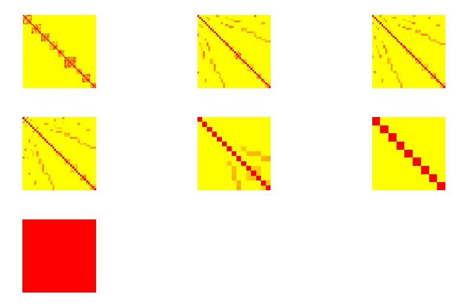


Figures 3 and 4 showcases the result of MH-KSC algorithm on the and respectively. From Figures 3(a) and 4(a), we observe the affinity matrices generated corresponding to the test set for and respectively. From Figures 3(b) and 4(b), we can observe the communities prevalent in the original network and the communities estimated by MH-KSC method for and respectively. In there are macro communities and micro communities while in there are macro communities and micro communities as depicted by Figures 3(b) and 4(b).
Table 1 illustrates the first levels of hierarchy for and and evaluates the clusters obtained at each level of hierarchy w.r.t. quality metrics , , and . Higher values of (close to ) and lower values of (close to ) represent good quality clusters. Both these external quality metrics are normalized as shown in [38]. Higher values of modularity ( close to ) and lower values of cut-conductance ( close to ) indicate better clustering information.
| Hierarchy | ||||||||||
|---|---|---|---|---|---|---|---|---|---|---|
| 10 | - | - | - | - | - | 134 | 0.685 | 0.612 | 0.66 | 1.98e-05 |
| 9 | - | - | - | - | - | 112 | 0.625 | 0.643 | 0.685 | 1.99e-05 |
| 8 | - | - | - | - | - | 106 | 0.61 | 0.667 | 0.691 | 1.99e-05 |
| 7 | 63 | 0.972 | 0.11 | 0.62 | 4.74e-04 | 103 | 0.595 | 0.692 | 0.694 | 1.98e-05 |
| 6 | 40 | 0.996 | 0.018 | 0.668 | 4.86e-04 | 97 | 0.53 | 0.77 | 0.706 | 1.99e-05 |
| 5 | 39 | 0.996 | 0.016 | 0.669 | 4.834e-04 | 87 | 0.47 | 0.90 | 0.722 | 1.99e-05 |
| 4 | 37 | 0.965 | 0.056 | 0.675 | 4.856e-04 | 44 | 0.636 | 0.74 | 0.773 | 1.99e-05 |
| 3 | 15 | 0.878 | 0.324 | 0.765 | 5.021e-04 | 13 | 1.0 | 0.0 | 0.82 | 2.0e-05 |
| 2 | 9 | 1.0 | 0.0 | 0.786 | 5.01e-04 | 5 | 0.12 | 1.643 | 0.376 | 2.12e-05 |
| 1 | 1 | 0.0 | 2.19 | 0.0 | 5.0e-04 | 1 | 0.0 | 2.544 | 0.0 | 2.0e-05 |
Table 2 provides the result of Louvain, Infomap and OSLOM methods and compares it with the best levels of hierarchy for and . The Louvain, Infomap and OSLOM methods require multiple runs as in each iteration they result in a different partition. We perform runs and report the mean results in Table 2. From Table 2, it can be observed that the best results for Louvain and Infomap methods generally occur at coarse levels of hierarchy w.r.t. to , and metric. Thus, these two methods work well to identify macro communities. The Louvain method works the better than MH-KSC for at macro and micro level. However, it cannot obtain similar quality micro communities when compared with MH-KSC method for as inferred from Table 2. The Infomap method performs the worst among all the methods w.r.t. detection of communities at finer levels of granularity. OSLOM performs well w.r.t. to locating both macro communities for and micro communities for as observed from Table 2. It performs better than any method w.r.t. locating micro communities for w.r.t. and metric. However, it performs worst while trying to identify the macro communities for the same benchmark network. The MH-KSC performs best on while it performs better w.r.t. locating macro communities for .
| Method | ||||||||||||
|---|---|---|---|---|---|---|---|---|---|---|---|---|
| Level | k | Level | k | |||||||||
| Louvain | 2 | 32 | 0.84 | 0.215 | 0.693 | 4.87e-05 | 3 | 135 | 0.853 | 0.396 | 0.687 | 1.98e-05 |
| 1 | 9 | 1.0 | 0.0 | 0.786 | 5.01e-04 | 1 | 13 | 1.0 | 0.0 | 0.82 | 2.0e-05 | |
| Infomap | 2 | 8 | 0.915 | 0.132 | 0.771 | 5.03e-04 | 3 | 590 | 0.003 | 8.58 | 0.003 | 1.98e-05 |
| 1 | 6 | 0.192 | 1.965 | 0.487 | 5.07e-04 | 1 | 13 | 1.0 | 0.0 | 0.82 | 2.0e-05 | |
| OSLOM | 2 | 38 | 0.988 | 0.037 | 0.655 | 4.839e-04 | 2 | 141 | 0.96 | 0.214 | 0.64 | 2.07e-05 |
| 1 | 9 | 1.0 | 0.0 | 0.786 | 5.01e-04 | 1 | 29 | 0.74 | 0.633 | 076 | 2.08e-05 | |
| MH-KSC | 5 | 39 | 0.996 | 0.016 | 0.67 | 4.83e-04 | 10 | 134 | 0.685 | 0.612 | 0.66 | 1.98e-05 |
| 2 | 9 | 1.0 | 0.0 | 0.786 | 5.01e-04 | 3 | 13 | 1.0 | 0.0 | 0.82 | 2.0e-05 | |
4.2 Real-Life Network Experiments
We experimented on real-life networks from the Stanford SNAP datasets http://snap.stanford.edu/data/index.html. These networks are anonymous networks and are converted to undirected and unweighted networks before performing experiments on them. Table 3 provides information about topological characteristics of these real-life networks. The Fb and Epn networks are social networks, PGP is a trust based network, Cond is a collaboration network between researchers, Enr is an email network, Imdb is an actor-actor collaboration network and Utube is a web graph depicting friendship between the users of Youtube.
| Network | Nodes | Edges | CCF |
|---|---|---|---|
| Facebook (Fb) | 4,039 | 88,234 | 0.6055 |
| PGPnet (PGP) | 10,876 | 39,994 | 0.008 |
| Cond-mat (Cond) | 23,133 | 186,936 | 0.6334 |
| Enron (Enr) | 36,692 | 367,662 | 0.497 |
| Epinions (Epn) | 75,879 | 508,837 | 0.1378 |
| Imdb-Actor (Imdb) | 383,640 | 1,342,595 | 0.453 |
| Youtube (Utube) | 1,134,890 | 2,987,624 | 0.081 |
In case of real-life networks the true hierarchical structure is not known beforehand. Hence, it is important to show whether they exhibit hierarchical organization which can be tested by identifying good quality clusters w.r.t. internal quality metrics like and at multiple levels of hierarchy.
We showcase the results for levels of hierarchy in a bottom-up fashion for the MH-KSC method in Table 4. The coarsest level of hierarchy has all nodes in one community and is not very insightful. Clusters at very coarse levels of granularity comprises giant connected components. So, it is more meaningful to give more emphasis to fine grained clusters at lower levels of hierarchy. To show that real-life networks exhibit hierarchy we evaluate our proposed MH-KSC approach in Table 4.
| Hierarchical Organization | |||||||||||
| Network | Metrics | Level 12 | Level 11 | Level 10 | Level 9 | Level 8 | Level 7 | Level 6 | Level 5 | Level 4 | Level 3 |
| 358 | 192 | 152 | 121 | 105 | 90 | 71 | 43 | 37 | 21 | ||
| Fb | 0.604 | 0.764 | 0.769 | 0.789 | 0.792 | 0.81 | 0.812 | 0.818 | 0.821 | 0.83 | |
| 2.47e-05 | 1.56e-04 | 2.38e-04 | 1.91e-04 | 1.95e-04 | 1.63e-04 | 2.16e-04 | 1.76e-04 | 2.44e-04 | 2.4e-04 | ||
| 345 | 274 | 202 | 156 | 129 | 83 | 59 | 46 | 24 | 19 | ||
| PGP | 0.682 | 0.693 | 0.705 | 0.715 | 0.725 | 0.727 | 0.728 | 0.729 | 0.701 | 0.698 | |
| 8.48e-05 | 9.84e-05 | 5.88e-05 | 1.38e-04 | 7.2e-05 | 8.03e-05 | 1.0e-04 | 1.07e-04 | 4.13e-04 | 4.89e-05 | ||
| 2676 | 1171 | 621 | 324 | 171 | 102 | 80 | 58 | 41 | 24 | ||
| Cond | 0.5 | 0.567 | 0.586 | 0.611 | 0.615 | 0.614 | 0.582 | 0.582 | 0.574 | 0.515 | |
| 2.49e-05 | 2.6e-05 | 3.7e-05 | 3.52e-05 | 3.6e-05 | 5.86e-05 | 2.37e-05 | 3.45e-05 | 1.43e-05 | 1.4e-05 | ||
| 2208 | 1002 | 464 | 303 | 211 | 163 | 119 | 76 | 59 | 48 | ||
| Enr | 0.30 | 0.388 | 0.444 | 0.451 | 0.454 | 0.427 | 0.43 | 0.325 | 0.328 | 0.271 | |
| 1.19e-05 | 3.18e-05 | 3.1e-05 | 5.3e-05 | 7.04e-05 | 2.69e-04 | 2.2e-03 | 1.651e-04 | 2.56e-05 | 5.46e-05 | ||
| 8808 | 3133 | 1964 | 957 | 351 | 220 | 166 | 97 | 66 | 26 | ||
| Epn | 0.105 | 0.156 | 0.158 | 0.176 | 0.184 | 0.183 | 0.186 | 0.184 | 0.146 | 0.006 | |
| 1.4e-06 | 3.1e-06 | 6.4e-06 | 7.0e-06 | 9.5e-06 | 1.26e-05 | 7.0e-06 | 9.0e-06 | 2.42e-05 | 7.8e-06 | ||
| 7431 | 1609 | 890 | 468 | 313 | 200 | 130 | 72 | 46 | 21 | ||
| Imdb | 0.357 | 0.47 | 0.473 | 0.485 | 0.503 | 0.521 | 0.508 | 0.514 | 0.513 | 0.406 | |
| 1.43e-06 | 2.78e-06 | 2.79e-06 | 5.6e-06 | 4.24e-06 | 5.6e-06 | 6.42e-06 | 1.99e-06 | 7.46e-06 | 9.2e-07 | ||
| 9984 | 2185 | 529 | 274 | 180 | 131 | 100 | 71 | 46 | 26 | ||
| Utube | 0.524 | 0.439 | 0.679 | 0.682 | 0.599 | 0.491 | 0.486 | 0.483 | 0.306 | 0.303 | |
| 2.65e-07 | 3.0e-07 | 1.3e-06 | 2.4e-06 | 1.0e-06 | 7.6e-06 | 1.03e-5 | 1.07e-05 | 2.33e-05 | 1.55e-04 | ||
| Hierarchical Organization | |||||||
|---|---|---|---|---|---|---|---|
| Network | Metrics | Level 6 | Level 5 | Level 4 | Level 3 | Level 2 | Level 1 |
| - | - | - | 225 | 155 | 151 | ||
| Fb | - | - | - | 0.82 | 0.846 | 0.847 | |
| - | - | - | 9.88e-05 | 1.33e-04 | 1.32e-04 | ||
| - | - | 2392 | 566 | 154 | 100 | ||
| PGP | - | - | 0.705 | 0.857 | 0.882 | 0.884 | |
| - | - | 4.95e-05 | 8.66e-05 | 6.8e-05 | 1.0e-04 | ||
| - | - | 6732 | 1825 | 1066 | 1011 | ||
| Cond | - | - | 0.56 | 0.7 | 0.731 | 0.732 | |
| - | - | 1.56e-05 | 2.97e-05 | 3.49e-05 | 4.15e-05 | ||
| - | - | 4001 | 1433 | 1237 | 1230 | ||
| Enr | - | - | 0.546 | 0.608 | 0.613 | 0.614 | |
| - | - | 1.28e-05 | 1.88e-05 | 4.58e-05 | 6.48e-05 | ||
| 10351 | 2818 | 1574 | 1325 | 1301 | 1300 | ||
| Epn | 0.287 | 0.319 | 0.323 | 0.324 | 0.324 | 0.324 | |
| 1.86e-06 | 4.2e-06 | 4.25e-06 | 5.57e-06 | 6.75e-06 | 1.13e-05 | ||
| - | 22613 | 4544 | 3910 | 3815 | 3804 | ||
| Imdb | - | 0.591 | 0.727 | 0.729 | 0.729 | 0.729 | |
| - | 1.0e-06 | 1.0e-06 | 1.85e-06 | 2.5e-06 | 2.82e-06 | ||
| 33623 | 11587 | 6964 | 6450 | 6369 | 6364 | ||
| Utube | 0.696 | 0.711 | 0.714 | 0.715 | 0.715 | 0.715 | |
| 1.38e-06 | 2.22e-06 | 3.25e-06 | 3.98e-06 | 4.06e-06 | 9.96e-06 | ||
| Infomap | OSLOM | |||||||
| Hierarchical Info | Hierarchical Info | |||||||
| Network | Metrics | Level 2 | Level 1 | Level 5 | Level 4 | Level 3 | Level 2 | Level 1 |
| 325 | 131 | - | 161 | 50 | 27 | 21 | ||
| Fb | 0.055 | 0.763 | - | 0.045 | 0.133 | 0.352 | 0.415 | |
| 2.86e-05 | 2.3e-04 | - | 2.0e-04 | 2.0e-04 | 3.0e-04 | 3.0e-04 | ||
| 85 | 65 | 431 | 143 | 51 | 48 | 45 | ||
| PGP | 0.041 | 0.862 | 0.748 | 0.799 | 0.709 | 0.709 | 0.709 | |
| 1.66e-04 | 1.40e-04 | 1.74e-04 | 5.32e-05 | 2.06e-04 | 1.56e-04 | 6.64e-05 | ||
| 1009 | 173 | 4092 | 2211 | 1745 | 1613 | 1468 | ||
| Cond | 0.648 | 0.027 | 0.483 | 0.574 | 0.615 | 0.615 | 0.05 | |
| 1.71e-05 | 2.78e-05 | 1.77e-05 | 2.48e-05 | 3.04e-05 | 6.56e-05 | 1.16e-05 | ||
| 1920 | 1084 | - | 3149 | 2177 | 2014 | 1970 | ||
| Enr | 0.015 | 0.151 | - | 0.317 | 0.382 | 0.412 | 0.442 | |
| 1.83e-05 | 8.39e-04 | - | 1.75e-05 | 4.96e-05 | 9.92e-05 | 7.22e-05 | ||
| 14170 | 50 | 1693 | 584 | 206 | 30 | 25 | ||
| Epn | 5.3e-06 | 4.48e-04 | 0.162 | 0.226 | 0.239 | 0.098 | 0.019 | |
| 3.97e-06 | 4.63e-05 | 1.23e-05 | 9.75e-06 | 2.45e-05 | 8.2e-06 | 7.9e-06 | ||
| 14308 | 3238 | - | 7469 | 2639 | 2017 | 2082 | ||
| Imdb | 0.04 | 0.707 | - | 0.045 | 0.092 | 0.1 | 0.115 | |
| 1.23e-06 | 4.72e-06 | - | 1.35e-06 | 2.03e-06 | 7.95r-06 | 1.17e-05 | ||
| 10703 | 976 | 18539 | 6547 | 4184 | 2003 | 1908 | ||
| Utube | 0.035 | 0.698 | 0.396 | 0.53 | 0.588 | 0.487 | 0.027 | |
| 1.38e-06 | 5.56e-06 | 1.52e-06 | 3.1e-07 | 2.72e-07 | 6.1e-06 | 5.69e-06 | ||
We compare MH-KSC algorithm with Louvain [15], Infomap [7] and OSLOM [21]. We perform runs for each of these methods as they generate a separate partition each time when they are executed. The mean results of Louvain method is reported in Table 5. Table 6 showcases the results for Infomap and OSLOM method.
From Table 5 it is evident that the Louvain method works best w.r.t. the modularity () criterion. This aligns with methodology as it is trying to optimize for . However, the Louvain method always performs worse than MH-KSC algorithm w.r.t. cut-conductance as observed from Tables 4 and 5. Another issue with the Louvain method is that except for the Fb and PGP networks it is not able to detect ( clusters) high quality clusters at coarser levels of granularity. This is attributed to the resolution limit problem suffered by Louvain method. From Table 6 we observe that the Infomap method produces only levels of hierarchy. In most of the cases, the clusters at one level of hierarchy perform good w.r.t. only quality metric except the PGP and Cond networks. The difference between the quality of the clusters at the levels of hierarchy is quite drastic. This reflects that the Infomap method is not very consistent w.r.t. various quality metrics.
We compare the performance of MH-KSC method with OSLOM in detail. From Tables 4 and 5 we observe that the MH-KSC technique outperforms OSLOM w.r.t. both quality metrics for Fb, Enr, Imdb and Utube networks while OSLOM does the same only for Cond network. In case of PGP, Cond and Epn networks OSLOM results in better than MH-KSC. However, MH-KSC approach has better value for PGP and Epn networks. For large scale networks like Enr, Imdb and Utube, OSLOM cannot identify good quality coarser clusters i.e. number of clusters detected are always .
4.3 Visualization and Illustrations
We provide a tree based visualization of the multilevel hierarchical organization for Fb and Enr networks in Figure 5. The hierarchial structure is depicted as tree for Fb and Enr network in Figures 5(a) and 5(b) respectively.


We plot the results corresponding to fine, intermediate and coarse levels of hierarchy for PGP network using the software provided in [21]. The software requires all the nodes in the network along with levels of hierarchy. In Figure 6 we plot the results for PGP net corresponding to MH-KSC algorithm using fine, intermediate and coarse levels of the hierarchical organization. For Louvain method we use and level of hierarchy as inputs for the finest level, and level of hierarchy as inputs for intermediate level and and level of hierarchy as inputs for coarsest level plot. The Infomap method only generates level of hierarchy which correspond to a coarse level plot. Similarly, for OSLOM we plot a fine and coarse level plot. The results for Louvain, Infomap and OSLOM methods are depicted in Figure 7.


.
Figures 6 and 7 shows that MH-KSC algorithm allows to depict richer structures than the other methods. It has more flexibility and allows the visualization at coarser, intermediate and finer levels of granularity. From Figures 7(a),7(b), 7(c) and Table 5, we observe that the Louvain method can only detect quality clusters at finer levels of granularity and cannot detect less than communities. While the Infomap method can only locate giant connected components for the PGP network as observed from Figure 7(d) and Table 6. The OSLOM method also seems to work reasonably well as observed from Figures 7(e) and 7(f). However, it detects fewer levels of hierarchy and thus has less flexibility in terms of selection for the level of hierarchy than the proposed MH-KSC approach.
We provide a visualization of the best layers of hierarchy for Epn network based on the and the criterion for MH-KSC, Louvain, Infomap and OSLOM methods respectively in Figures 8 and 9. The result for Infomap method in both the figures is the same as it only generates levels of hierarchy.


5 Conclusion
We proposed a new multilevel hierarchical kernel spectral clustering (MH-KSC) algorithm. The approach relies on the KSC primal-dual formulation and exploits the structure of the projections in the eigenspace. The projections of the validation set provided a set ( ) of increasing distance thresholds. These distance thresholds were used along with affinity matrix obtained from the projections in an iterative procedure to obtain a multilevel hierarchical organization in a bottom-up fashion. We highlighted some of the necessary conditions for the feasibility of the approach to large scale networks. We showed that many real-life networks exhibit hierarchical structure. Our proposed approach was able to identify good quality clusters for both coarse as well as fine levels of granularity. We compared and evaluated our MH-KSC approach against several state-of-the-art large scale hierarchical community detection techniques.
Acknowledgements
This work was supported by Research Council KUL: ERC AdG A-DATADRIVE-B, GOA/11/05 Ambiorics, GOA/10/09MaNet, CoE EF/05/006 Optimization in Engineering(OPTEC), IOF-SCORES4CHEM, several PhD/postdoc and fellow grants; Flemish Government:FWO: PhD/postdoc grants, projects: G0226.06 (cooperative systems & optimization), G0321.06 (Tensors), G.0302.07 (SVM/Kernel), G.0320.08 (convex MPC), G.0558.08 (Robust MHE), G.0557.08 (Glycemia2), G.0588.09 (Brain-machine) G.0377. 12 (structured models) research communities (WOG:ICCoS, ANMMM, MLDM); G.0377.09 (Mechatronics MPC) IWT: PhD Grants, Eureka-Flite, SBO LeCoPro, SBO Climaqs, SBO POM, O&O-Dsquare; Belgian Federal Science Policy Office: IUAP P6/04 ( DYSCO, Dynamical systems, control and optimization, 2007-2011); EU: ERNSI; FP7-HD-MPC (INFSO-ICT-223854), COST intelliCIS, FP7-EMBOCON (ICT-248940); Contract Research: AMINAL; Other:Helmholtz: viCERP, ACCM, Bauknecht, Hoerbiger. Johan Suykens is a professor at the KU Leuven, Belgium.
References
- [1] Barabsi, A., Albert, R.; Emergence of scaling in random networks. Science, 1999, 286(5439), 509-512.
- [2] Clauset, A., Cosma Rohilla, S., Newman, M.; Power-law distribution in empirical data. SIAM Review, 2009, 51, 661-703.
- [3] Girvan, M., Newman, M.E.; Community structure in social and biological networks. PNAS, 2002, 99(12), 7821-7826.
- [4] Fortunato, S.; Community detection in graphs. Physics Reports, 2009, 486, 75-174.
- [5] Danaon, L., Diz-Guilera, A., Duch, J., Arenas, A.; Comparing community structure identification. Journal of Statistical Mechanics: Theory and Experiment, 2005, 09(P09008+).
- [6] Clauset, A., Newman, M.E., Moore, C.; Finding community structure in very large scale networks. Physical Review E, 2004, 70(066111).
- [7] Rosvall, M. and Bergstrom, C.; Maps of random walks on complex networks reveal community structure. PNAS, 2008, 105, 1118-1123.
- [8] Schaeffer, S.; Algorithms for Nonuniform Networks. Phd thesis, Helsinki University of Technology, 2006.
- [9] Lancichinetti, A., Fortunato, S.; Community detection algorithms: a comparitive analysis. Physical Review E, 2009, 80(056117).
- [10] Ng, A.Y., Jordan, M.I., Weiss, Y.; On spectral clustering: analysis and an algorithm, In Proceedings of the Advances in Neural Information Processing Systems; Dietterich, T.G., Becker, S., Ghahramani, Z., editors ;MIT Press: Cambridge, MA, 2002, pp. 849-856.
- [11] Shi, J., Malik, J.; Normalized cuts and image segmentation. IEEE Transactions on Pattern Analysis and Intelligence, 2000, 22(8), 888-905.
- [12] von Luxburg, U.; A tutorial on Spectral clustering. Stat. Comput, 17, 395-416.
- [13] Chung, F.R.K.; Spectral Graph Theory. American Mathematical Society, 1997.
- [14] Zelnik-Manor, L., Perona, P.; Self-tuning spectral clustering. Advances in Neural Information Processing Systems; Saul, L.K., Weiss, Y., Bottou, L., editors; MIT Press: Cambridge, MA, 2005; pp. 1601-1608.
- [15] Blondel, V., Guillaume, J., Lambiotte, R., Lefebvre, L.; Fast unfolding of communities in large networks. Journal of Statistical Mechanics: Theory and Experiment, 2008, 10:P10008.
- [16] Newman, M.E.; Analysis of weighted networks. Physical Review E, 2004, 70(056131).
- [17] Fortunato, S., Barthlemy, M.; Resolution limit in community detection. PNAS, 2007, 104(36).
- [18] Kumpula, M., Saramaki, J., Kaski, K., Kertesz, J.; Limited resolution and multiresolution methods in complex network community detection. Fluctuation Noise Letters, 2007, 7(209).
- [19] Good, H., de Montjoye, A., Clauset, A.; Performance of modularity maximization in practical contexts. Physical Review E, 2010, 81(046106).
- [20] Lanchichinetti, A., Fortunato, S.; Limits of modularity maximization in community detection. Physical Review E, 2011, 84(066122).
- [21] Lanchichinetti, A., Radicchi, F., Ramasco, J., Fortunato, S.; Finding statistically significant communities in networks. Plos One, 2011, 6(e18961).
- [22] Alzate, C., Suykens, J.A.K.; Multiway spectral clustering with out-of-sample extensions through weighted kernel PCA. IEEE Transactions on Pattern Analysis and Machine Intelligence, 2010, 32(2), 335-347.
- [23] Suykens, J.A.K., Van Gestel, T., De Brabanter, J., De Moor, B., Vandewalle, J.; Least squares support vector machines. World Scientific, 2002.
- [24] Langone, R., Alzate, C., Suykens, J.A.K.; Kernel spectral clustering for community detection in complex networks. In IEEE WCCI/IJCNN, 2012, 2596-2603.
- [25] Mall, R., Langone, R., Suykens, J.A.K.; Kernel Spectral Clustering for Big Data Networks, Entropy (Special Issue: Big Data), 2013, 15(5), 1567-1586.
- [26] Mall, R., Langone, R., Suykens, J.A.K.; FURS: Fast and Unique Representative Subset selection retaining large scale community structure. Social Network Analysis and Mining, 2013, 3(4), 1075-1095.
- [27] Mall, R., Langone, R., Suykens, J.A.K.; Self-Tuned Kernel Spectral Clustering for Large Scale Networks. In Proceedings of the IEEE International Conference on Big Data (IEEE BigData 2013), 2013, pp. 385-393.
- [28] Mall, R., Suykens, J.A.K.; Very sparse LSSVM reductions to large scale data. IEEE Transactions on Neural Networks and Learning Systems, in press.
- [29] Mall, R., Suykens, J.A.K.; Sparse Reductions for Fixed-Size Least Squares Support Vector Machines on Large Scale Data. In Proc. of Pacific-Asia Conference on Knowledge Discovery and Data Mining (PAKDD), 2013, pp. 161-173.
- [30] Mall, R., El Anbari, M., Bensmail H., Suykens, J.A.K.; Primal-dual framework for Feature Selection using Least Squares Support Vector Machines. In Proc. of the International Conference on Management of Data (COMAD), 2013, pp. 105-108.
- [31] Mall, R., Langone R., Suykens, J.A.K.; Highly Sparse Reductions to Kernel Spectral Clustering. In Proc. of the International Conference on Pattern Recognition and Machine Intelligence (PREMI), 2013, pp. 163-169.
- [32] Mall, R., Mehrkanoon S., Langone, R., Suykens, J.A.K.; Optimal Reduced Set for Sparse Kernel Spectral Clustering. IJCNN 2014, pp. 2436-2443.
- [33] Alzate, C., Suykens, J.A.K.; Hierarchical kernel spectral clustering. Neural Networks, 2012, 35, 21-30.
- [34] Dhillon, I., Guan, Y., Kulis, B.; Weighted Graph Cuts without Eigenvectors: A Multilevel Approach. IEEE Transactions on Pattern Analysis and Machine Intelligence, 2007, 29(11), 1944-1957.
- [35] Karypis, G., Kumar, V.; A fast and high quality multilevel scheme for partitioning irregular graphs. SIAM J. Scientific Computing, 1999, 20(1), 359-392.
- [36] Kushnir, D., Galun, M., Brandt, A.; Fast multiscale clustering and manifold identification. Pattern Recognition, 2006, 39(10), 1876-1891.
- [37] Leskovec, J., Faloutsos, C.; Sampling from large graphs. KDD, 2006, pp. 631-636.
- [38] Rabbany, R., Takaffoli, M., Fagnan, J., Zaiane, O.R., Campello R.J.G.B.; Relative Validity Criteria for Community Mining Algorithms. 2012, International Conference on Advances in Social Networks Analysis and Mining (ASONAM), pp. 258-265.
- [39] Lamirel, J.C., Mall, R., Cuxac, P., Safi, G.; A New Efficient and Unbiased Approach for Clustering Quality Evaluation. PAKDD Workshops, 2011, pp. 209-220.