Early-time VLA observations and broad-band afterglow analysis
of
the Fermi-LAT detected GRB 130907A
Abstract
We present multi-wavelength observations of the hyper-energetic gamma-ray burst (GRB) 130907A, a Swift -discovered burst with early radio observations starting at hr after the -ray trigger. GRB 130907A was also detected by the Fermi/LAT instrument and, at late times, showed a strong spectral evolution in X-rays. We focus on the early-time radio observations, especially at , to attempt identifying reverse shock signatures. While our radio follow-up of GRB 130907A ranks among the earliest observations of a GRB with the Karl G. Jansky Very Large Array (VLA), we did not see an unambiguous signature of a reverse shock. While a model with both reverse and forward-shock can correctly describe the observations, the data is not constraining enough to decide upon the presence of the reverse-shock component. We model the broad-band data using a simple forward-shock synchrotron scenario with a transition from a wind environment to a constant density interstellar medium (ISM) in order to account for the observed features. Within the confines of this model, we also derive the underlying physical parameters of the fireball, which are within typical ranges except for the wind density parameter (), which is higher than those for bursts with wind-ISM transition, but typical for the general population of bursts. We note the importance of early-time radio observations of the afterglow (and of well sampled light curves) to unambiguously identify the potential contribution of the reverse shock.
I. Introduction
Gamma-ray bursts’ afterglows still pose some fundamental unanswered questions. The processes giving rise to prompt and early-afterglow emission at optical and radio frequencies are among the least well understood. Early-time optical [1] and radio [50] flashes were first discovered in GRB 990123 and attributed to reverse-shock emission [64, 88, 12, 98, e.g.]. But, later on, fast robotic telescopes did not find evidence for early optical flashes in the expected numbers [62]. It has been suggested that the lack of early optical emission may be due to the fact that the reverse shock peaks below the optical range, at mm or cm wavelengths [50, 11, 56, 83]. Another possibility is that the reverse shock is entirely suppressed by e.g. a high degree of magnetization of the ejecta [121].
Here, we present early-time radio observations of GRB 130907A, together with observations at other wavelengths. Our radio follow-up of GRB 130907A ranks among the earliest observations of a GRB with the VLA. However, our data do not show a clear reverse shock signature. Besides an early-time radio follow-up and a self-absorbed radio spectrum, the other interesting features of this burst consist of an early-time Fermi/LAT detection and a significant late-time spectral evolution in the X-ray band.
Our paper is organized as follows. In Section II we present the observational data for this burst and discuss the spectral and temporal properties of GRB 130907A. In Section III we provide a theoretical interpretation for the broad-band data, and conclude in Section IV. In this paper, we use the notation ( is the temporal index and is the spectral index) and for any physical quantity in cgs units (unless otherwise stated).
II. Observations and data analysis
II.1. Gamma-rays
GRB 130907A [69], was discovered by the BAT instrument aboard the Swift satellite [34] at 21:41:13 UT. It was also detected by the Fermi/LAT [103], Konus WIND [36], and various ground-based observatories at longer wavelengths [37, 14, e.g.]. With a redshift of , this GRB occurred at a luminosity distance of [19], calculated using the following cosmological parameters: , and . The isotropically emitted energy is (calculated from 1 keV to 10 MeV in the local frame). The jet opening angle (, see Section III.4) corrected energy is erg, which makes this burst part of the hyper-energetic class of GRBs [10]. Moreover, at 18 ks after the -ray trigger, the Fermi/LAT detected one of the highest-energy (55 GeV) photons ever observed in a GRB [103]. We refer the reader to Tang et al. [94] for more details about the LAT flux measurements.
II.2. X-rays
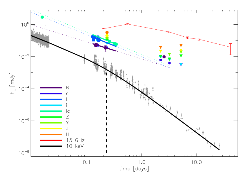
X-ray measurements by Swift /XRT of GRB 130907A started at s after the trigger (during the burst prompt -ray emission phase) and lasted until d after the burst. The light curve is overall declining with an easily identifiable break around 0.2 d since trigger (Figure 1), and a strong spectral evolution at late times (Figure 2). Due to this spectral evolution, we used a dynamic count-to-flux density conversion and derived an accurate light curve using the burst analyser [21, 23].
The 10 keV light curve of GRB 130907A shows a clear break followed by a steepening of the temporal decay index (Figure 1). In what follows, for our analysis of the afterglow, we discard all observations at due to possible contribution of the prompt emission. By fitting the X-ray light curve with a smoothly broken power-law of the form [5] we get days and indices: and , respectively before and after the break. We did not attempt to find the parameter responsible for the smoothness of the break and fixed it to the nominal value of 1 [5, the parameter in]. This could tentatively explain why the fit underestimated the points close to the break.
We have obtained the spectral data from the XRT repository’s spectral tools11 1 http://www.swift.ac.uk/xrt_spectra. The spectral index before the temporal break is unusually hard, with no significant evolution. A unique feature of the X-ray afterglow is the spectral evolution starting with the light curve break, from at early times to at later times (see Figure 2). A linear fit (in ) to the first three points gives a slope of , consistent with no spectral evolution, while for the last four points the slope is indicative of an evolving spectral index. The average spectral index after the break is . The X-ray absorbing column of the host galaxy is: .

We finally note that the light curve integrated for the entire energy interval of XRT (0.3-10 keV) has a different behavior than the flux density light curve plotted in Figure 1. Indeed, the automatic fitting routine [22] yields a broken power-law fit with three breaks for the integrated light curve (see http://www.swift.ac.uk/xrt_live_cat/00569992/). On the other hand, a fit with a smoothly broken power-law function (similar to the one we fitted to the flux density light curve) does not constrain the break time, while a simple power-law fit gives a slope of . The latter is in strong contrast with the steep slope found for the late-time flux density (Figure 1), and it is indicative of a changing X-ray spectrum at late times.
II.3. Optical
We gathered the optical observations of GRB 130907A from the public GCN bulletins (see Table 1). In case of Skynet observations, where the data points were reported on figures, we obtained the numerical flux values by digitizing these figures.
We correct the optical data of GRB 130907A for Galactic absorption ( mag) in the direction of the burst using the maps of Schlafly & Finkbeiner [91]. We find that the optical spectral index at the time of the first radio observation is , suggesting that the host galaxy strongly absorbs the optical flux. We fit the I, Ic and R filter measurements from d to d to obtain the temporal decay index for this time interval (Figure 1), and we get (from 7 measurements; Table 1), (from 3 measurements; Table 1), and (from 3 measurements; Table 1). The other optical observations, at earlier and later times, are too sparse to derive secure spectral or temporal information. We note, however, that late-time measurements seem to lie above the extrapolation from the temporal decay derived between d to d, thus suggesting a late-time flattening (Figure 1). A foreground galaxy (SDSS J142333.95+453626.2 with photometric redshift ) at a distance of from GRB 130907A has been identified by Lee et al. [60] with and magnitudes comparable to that of the afterglow at days after the trigger. This galaxy could tentatively explain the flattening of the optical afterglow at these late times. On the other hand, Butler et al. [8] have limited the contribution of galaxy flux in - and bands to 22.6 mag.
To account for the extinction (reddening) in the host galaxy, we use the absorption curves of [39]. The relation between the absorbed and unabsorbed flux is: . Here, is the absorption curve, characterized by a -band value, , which is a free parameter, and a shape which is usually taken to be similar to the LMC, SMC or the Milky Way. Due to the small number of optical observations, we assume the SMC extinction curve, which is most commonly used for GRB afterglow studies [90]. We have the best spectral coverage in the optical band around the time of Epoch I ( days), where we have extrapolated the available filters (R, Rc, I, Ic) from to days. By further assuming that the optical and X-ray spectral indices are the same (; at this early time there is no significant spectral evolution in X-rays, and the optical and X-ray temporal slopes are consistent with being the same within the large uncertainties) we find in the frame of the host galaxy (see Figure 3).

The above value of is derived by fitting a power law with the same spectral index as the X-ray measurements to the unabsorbed optical points. Indeed, we can exclude a spectral break between the optical and X-ray regimes: If there was a break, the optical spectral index would be which, after correction for extinction, would imply a true optical flux incompatible with the X-ray data.
Using the X-ray spectral analysis described in Section II.2, we estimate . This value is on the lower side, but still consistent with, the distribution reported in [90]. Generally speaking, GRB host galaxies have systematically larger ratios compared to the Magellanic clouds and the Milky Way [90], and this effect is at least partly intrinsic to the host galaxies. Bearing in mind the uncertainties on due to the small number of optical measurements, the value of the host galaxy of GRB 130907A is more like the SMC than for most GRB sightlines.
II.4. Radio
Radio observations of GRB 130907A were performed with the VLA22 2 The National Radio Astronomy Observatory is a facility of the National Science Foundation operated under cooperative agreement by Associated Universities, Inc.; http://www.nrao.edu/index.php/about/facilities/vlaevla [75] in its CnB and B configurations, under our Target of Opportunity programs33 3 VLA/13A-430 - PI: A. Corsi; VLA/S50386 - PI: S.B. Cenko.
Our observations of GRB 130907A rank among the earliest VLA detections of a GRB (see Figure 4). The follow-up started at hours after the trigger. Hereafter, we refer to the first VLA observation as Epoch I or EI; later VLA observations are labeled incrementally up to Epoch V at 42 d after the trigger (Table 2).


VLA data were reduced and imaged using the Common Astronomy Software Applications (CASA) package. Specifically, the calibration was performed using the VLA calibration pipeline v1.2.0. After running the pipeline, we inspected the data (calibrators and target source) and applied further flagging when needed. 3C286 and J1423+4802 were used as flux and phase calibrators, respectively. The VLA measurement errors are a combination of the rms map error, which measures the contribution of small unresolved fluctuations in the background emission and random map fluctuations due to receiver noise, and a basic fractional error [67, here conservatively estimated to be , based on the flux variations measured for the phase calibrator;] which accounts for inaccuracies of the flux density calibration. Theses errors were added in quadrature and total errors are reported in Table 2. An additional source of error in the radio band can occur from scintillation, which we discuss in Section III.5.
We also observed the position of GRB 130907A with the Combined Array for Research in Millimeter Astronomy (CARMA) on 2013-09-08 between 21:46:36 and 23:12:35 UT ( day). Observations were conducted in single-polarization mode with the 3 mm receivers tuned to a frequency of 93 GHz, and were reduced using the Multichannel Image Reconstruction, Image Analysis and Display environment (MIRIAD). Flux calibration was established by a short observation of Mars at the beginning of the track. We detect no source at the location of the GRB afterglow in the reduced image, with a limiting flux of 1.1 mJy (2).

During Epoch I, the radio spectral index is , which strongly suggests that Epoch I is self-absorbed. As evident from Figure 5, at later times our VLA observations suggest an evolution of the radio emission toward an optically thin regime, with the spectral index progressively becoming flatter with time. In order to extract from our data a well sampled radio light curve, we have extrapolated VLA measurements at various epochs to 15 GHz using the best fitting power law to the spectra at a given epoch (Table 2). For fitting purposes, we set the initial light curve slope to , corresponding to the temporal behavior expected for a fireball expanding in a wind environment (see Section III). With this choice, we find for the late-time temporal slope at 15 GHz, and a peak-time of days (Figure 6).

| Timemid[days] | Filter | mag[AB] | Instrument | Reference |
| r | 15 (0.2) | MASTER | (1) | |
| 0.0152 | Ic | 15.26 0.03 | Tautenburg | (2) |
| 0.0172 | Rc | 16.57 0.03 | Tautenburg | (2) |
| 0.127 | I | 18.27 0.15 | Skynet | (3) |
| 0.131 | I | 18.76 0.23 | Skynet | (3) |
| 0.132 | I | 18.41 0.084 | Skynet | (4) |
| 0.136 | I | 18.40 0.12 | Skynet | (3) |
| 0.144 | R | 19.65 0.20 | Skynet | (3) |
| 0.148 | R | 19.51 0.13 | Skynet | (4) |
| 0.154 | i’ | 18.86 0.09 | Skynet | (4) |
| 0.158 | I | 18.35 0.13 | Skynet | (3) |
| 0.159 | r’ | 19.65 0.10 | Skynet | (4) |
| 0.164 | I | 18.91 0.16 | Skynet | (3) |
| 0.167 | I | 18.79 0.09 | Skynet | (4) |
| 0.217 | R | 20.06 0.47 | T21 | (5) |
| 0.232 | r | 20.01 0.03 | RATIR | (6) |
| 0.232 | i | 19.30 0.02 | RATIR | (6) |
| 0.258 | Ic | 19.05 0.09 | Skynet | (4) |
| 0.287 | Rc | 19.91 0.11 | Skynet | (4) |
| 0.316 | Ic | 19.31 0.13 | Skynet | (4) |
| 0.341 | Ic | 19.51 0.22 | Skynet | (4) |
| 2.22 | r | 21.92 0.12 | RATIR | (7) |
| 2.22 | i | 21.38 0.09 | RATIR | (7) |
| 2.56 | R | 21.44 0.16 | Maidanak | (8) |
| 3.22 | r | 22.40 0.14 | RATIR | (9) |
| 3.22 | i | 21.73 0.10 | RATIR | (9) |
| 8.56 | white | 15.45 0.02 | UVOT | (10) |
| 7.13 | v | 16.29 0.16 | UVOT | (10) |
| 6.27 | b | 16.78 0.12 | UVOT | (10) |
| 3.31 | u | 15.87 0.04 | UVOT | (10) |
| 7.71 | w1 | 18.54 0.31 | UVOT | (10) |
| 7.42 | m2 | 19.20 | UVOT | (10) |
| 6.85 | w2 | 18.70 | UVOT | (10) |
| 0.232 | Z | 18.78 0.05 | RATIR | (6) |
| 0.232 | Y | 18.48 0.06 | RATIR | (6) |
| 0.232 | J | 18.13 0.06 | RATIR | (6) |
| 0.232 | H | 17.63 0.05 | RATIR | (6) |
| 2.22 | Z | 21.37 | RATIR | (7) |
| 2.22 | Y | 20.87 | RATIR | (7) |
| 2.22 | J | 20.58 | RATIR | (7) |
| 2.22 | H | 19.97 | RATIR | (7) |
| 3.22 | Z | 21.80 | RATIR | (7) |
| 3.22 | Y | 21.05 | RATIR | (7) |
| 5.23 | r | 22.68 | RATIR | (11) |
| 5.23 | i | 22.62 | RATIR | (11) |
| 5.23 | Z | 21.30 | RATIR | (11) |
| 5.23 | Y | 20.70 | RATIR | (11) |
| 5.23 | J | 20.42 | RATIR | (11) |
| 5.23 | H | 19.69 | RATIR | (11) |
| Timemid [days] | [GHz] | Flux [Jy] | Instrument | Reference |
|---|---|---|---|---|
| 0.193 (EI) | 19.2 | 630 25 | EVLA | (this work) |
| 0.193 (EI) | 24.5 | 1160 28 | EVLA | (this work) |
| 0.550 | 15 | 1060 110 | AMI | (1) |
| 1.03 | 93 | 1100 (2) | CARMA | (this work) |
| 1.735 | 5 | 190 30 | WSRT | (2) |
| 3.08 (EII) | 8.5 | 441 34 | EVLA | (this work) |
| 3.08 (EII) | 11 | 444 45 | EVLA | (this work) |
| 3.08 (EII) | 13.5 | 347 24 | EVLA | (this work) |
| 3.08 (EII) | 16 | 358 43 | EVLA | (this work) |
| 6.86 (EIII) | 5 | 204 22 | EVLA | (this work) |
| 6.86 (EIII) | 7.4 | 93 21 | EVLA | (this work) |
| 6.86 (EIII) | 8.5 | 208 16 | EVLA | (this work) |
| 6.86 (EIII) | 11 | 152 20 | EVLA | (this work) |
| 11.15 (EIV) | 13.5 | 155 24 | EVLA | (this work) |
| 11.15 (EIV) | 16 | 109 21 | EVLA | (this work) |
| 41.96 (EV) | 5 | 62 12 | EVLA | (this work) |
| 41.96 (EV) | 7.4 | 45 10 | EVLA | (this work) |
| 41.96 (EV) | 8.5 | 61 26 | EVLA | (this work) |
| 41.96 (EV) | 11 | 72 19 | EVLA | (this work) |
II.5. Radio-to-GeV spectral energy distribution
During Epoch I, defined by the time of the first VLA observation, we have a spectral coverage spanning orders of magnitude from radio to -rays (Figure 7). The spectral index in the radio band is , which indicates that the radio emission is self-absorbed at this epoch (Section II.4). We extrapolate the optical measurements to Epoch I using the temporal indices as derived in Section II.3, i.e. . The break in the spectrum at the intersection of the extrapolated radio and optical measurements, occurs at .
In the X-rays, the spectral and temporal slopes during Epoch I are and , respectively (see Section II.2). The emission in the LAT energy band has a temporal index of [94], which is consistent with the X-ray one within the large uncertainties.
Interestingly, the spectrum at Epoch I is consistent with a single power-law component (dashed line in Figure 7) from optical to the GeV range. It should be noted, however, that the low photon counts do not allow to derive a spectral index for the GeV emission, thus a spectral break might be present between the X-rays and the GeV range (dotted line in Figure 7). In other words, the consistency of the X-ray and GeV (LAT) temporal indices does not require the presence of a spectral break, but the uncertainties in the LAT flux do not exclude the presence of a cooling break () between the X-rays and GeV band. In fact, as we discuss in Section III.8, a cooling break just above the X-ray band during Epoch I (dotted line) helps explain the late-time spectral evolution observed in X-rays. The presence of such a break would cause the LAT flux to be slightly underpredicted (by ), but this could be mitigated by invoking an emergent SSC component [94, as suggested by].

III. Modeling
III.1. Initial considerations
We assume the radiation originates from synchrotron radiation of shock accelerated electrons. The electrons have a distribution described by a broken power-law. The resulting synchrotron spectrum is also a set of joined power-laws with breaks at the characteristic frequencies: the injection frequency, , where the bulk of the electrons radiate; the cooling frequency, , where the cooling time of the electron radiating at this frequency is equal to the dynamical time; and the self-absorption frequency, , which is defined as the frequency where the optical depth for synchrotron photons becomes greater than unity for scattering on the synchrotron emitting electrons [63, 89, 40].
First, inspecting the general properties of the multi-wavelength afterglow observations, this burst presents a conundrum. As we explain in what follows, based on the closure relations between the temporal and spectral indices for GRBs [86, see e.g. ], the early () X-ray light curve slope is suggestive of a wind environment and consistent with the optical measurements. On the other hand, the radio observations are better explained in an ISM (Section III.2). Finally, the late-time X-ray light curve has a steep slope (Figure 1) and a strong spectral evolution (Figure 2) indicating the passage of a characteristic frequency through the X-ray band (although the steep slope of the X-ray light curve is difficult to explain in both an ISM and a wind environment).
We thus suggest that a simple external-shock model is not able to account for all the observed data. Among the multitude of extensions to the simplest model, a possible explanation is that GRB 130907A is produced by a shock initially propagating in a wind environment, which then transitions to a constant density ISM. Similar models were proposed by e.g. Wijers [105], Peer & Wijers [74], Gendre et al. [35], Kamble et al. [47]. Hereafter we assume that the spectral evolution observed in the late-time X-ray afterglow is due to the passage of a characteristic frequency in band. However, we also note that the higher-than-average reddening observed in GRB 130907A suggests this burst might be a good candidate for the dust screen scenario proposed by Evans et al. [24] to explain the spectral evolution observed in X-rays for GRB 130925A.
As the blast wave transitions from a wind to an ISM environment, roughly at the time of the X-ray break, the cooling frequency () sweeps through the X-rays causing the observed spectral evolution. The passage of the cooling frequency will not affect the radio light curve which behaves simply as in the case of an ISM.
By looking at the 15 GHz light curve (Figure 6), we find no obvious requirement to include a reverse shock in our modeling. However, the behavior of the 5 GHz flux seems to favor a forward-plus-reverse-shock model. A better temporal coverage, particularly between 1 d and 2 d since trigger at the highest radio frequencies, would likely have allowed us to securely discriminate between a forward-shock-only and a forward-plus-reverse-shock scenario.
III.2. Early-time wind profile
If we assume that, before the temporal break (), the X-ray band is below the cooling frequency and above the self-absorption and injection frequencies (), based on the spectral and temporal indices, we can estimate the nature of the interstellar matter density profile () e.g. from Sari & Mészáros [87]: , which is suggestive of a wind environment before 44 4 For a detailed treatment of the radiation from GRB afterglows in a general circumstellar density profile, see Yi et al. [107].. This results in a power-law index of the electron distribution of ().
The temporal evolution of the cooling frequency is , where , for a circumstellar density profile index . Thus, the cooling break is almost constant with time, similarly to what was found by Perley et al. [83] in the case of GRB 130427A.
The self-absorbed spectrum at Epoch I is a noteworthy feature of this burst, and the spectral index is is unique: The more commonly discussed cases for synchrotron emission have a self-absorbed slope of [108, e.g.]. The evolution of the self-absorption frequency provides another argument in favor of the wind nature of the environment closer to the explosion site. At Epoch I, GHz (though this value should be considered uncertain due to the extrapolation over many orders of magnitude; see Figure 7 and Section II.5). Epoch II is clearly not self-absorbed (Figure 5), thus GHz. In an ISM environment, , which yields a GHz for between 2 and 3. On the other hand, for a wind environment, , which yields a self-absorption frequency below 10 GHz at Epoch II, in agreement with our observations.
We finally note that a more common self-absorbed spectral slope of , which would be expected in the regime, would be consistent with the observed value of only at the level. In this regime, because the later epochs are not self-absorbed, would need to pass in the radio band by the time of Epoch II. In the ISM case, while in the wind case . Thus, our conclusion favoring an initial wind environment is not affected by the relative ordering of and .
III.3. Spectral energy distribution at Epoch I
The spectrum at Epoch I suggests a synchrotron origin for the entire spectral range [51, 49, see e.g. ]. However, in a synchrotron model one has to overcome the maximum attainable synchrotron energy condition, which might pose a problem for a synchrotron-only model [18]. A scenario for interpreting Epoch I spectrum with a forward-shock synchrotron component is in the regime where: (dotted line in Figure 7). Although observations are equally consistent with (dashed line in Figure 7), the spectral evolution observed in the late-time X-ray light curve favors a model where lies just above the Swift/XRT range during Epoch I (Section III.4). For the implications of an alternative inverse-Compton model, see: Tang et al. [94].
III.4. ISM transition and origin of the X-ray break
The break observed in X-rays (Figure 1) is clearly inconsistent with a jet break because it is chromatic: It only occurs in X-rays, the radio component does not have a break, while the optical measurements do not support it. Chromatic breaks are not uncommon in GRB afterglows [73, 61, see e.g. ], but are not generally accompanied by spectral evolution.
No clear achromatic break can be identified in the X-ray light curve until about 20 d since explosion. By imposing d, we get and a beaming-corrected energy of .
To account for the observed spectral evolution, we assume the cooling frequency starts to cross the Swift/XRT band at about the same time the shock reaches the transition from the wind environment to the ISM. This requires that the cooling break lies just above the XRT range during Epoch I, since in a medium is almost constant with time (Section III.2), while in an ISM. Indeed, the Swift/XRT data imply that takes about two orders of magnitude in time (from to ) to move through approximately one order of magnitude in frequency (from 10 keV to 0.3 keV, the range of XRT; see Figure 2). Moreover, the observed change in spectral slope, , is consistent with the theoretical expectations for the passage of in band, (Figure 2). We note that a constant density medium might not necessarily be related to ISM, but it might also result from the interaction of the stellar wind with the circumstellar environment. The latter may indeed be homogenized by this interaction, as suggested by several studies [101, e.g.].
Last but not least, a transition from a wind-like () medium to an ISM also allows us to explain the observed late-time slope of the radio light curve. Indeed, for a medium to yield a radio temporal slope of (Section II.4), one needs an electron distribution index of 55 5 In order to obtain a finite energy in electrons it is usual to assume . See however Panaitescu [70] for a treatment of a case.. On the other hand, in an ISM, the observed late-time radio light curve slope implies , which is consistent with the value independently derived from the early-time X-ray observations (Section III.2).
A shortcoming of our presented model is that the X-ray temporal slope after the break is steeper than expected for a transition of the cooling frequency. In the framework of a simple synchrotron model the steepest temporal decay index is and it does not depend on the nature of the environment. This expression for a temporal index applied to the X-ray data yields , which is an unusually steep value for the electron distribution index.
With the introduction of a narrow jet responsible for the X-ray emission and a wider jet for the longer wavelength afterglow [85, 99], one would decouple the X-ray and optical/radio behavior. This way a break in the X-ray would be due to the narrow jet with opening angle , and energy release corrected for beaming of . This is the opening angle and the beaming corrected energy respectively if we interpret the break in X-ray as a jet break. The consequent passing of the cooling frequency would explain the spectral evolution. The radio and optical fluxes would be due to synchrotron radiation from a wider jet. This would naturally explain the late behavior of the X-ray light curve with , as the post jet-break phase flux evolves as . We consider this model lacks solid observational evidence, but can be substantiated for similar future bursts with better temporal coverage of the emission.
There are other possible solutions to the puzzling late-time behavior of GRB 130907A X-ray light curve (see Section III.4): the break in the light curve can be attributed to the end of the shallow decay (plateau) phase [66, 61] of the GRB. It is uncommon, but not impossible that the plateau phase has a temporal index of [41, see Figure 4 in]. In this case the flux before the break is related to central engine activity, and the evidence for an initial wind environment is not as compelling. The discrepancy between the late radio and X-ray temporal indices is still too large to be solved by this model.
A rather contrived setup would ascribe the radio emission to the usual synchrotron component propagating in the ISM and the X-ray flux would be given by synchrotron self-Compton radiation. The self-Compton light curves can be as steep as for ISM to in wind case. It is not possible to constrain a self-Compton component form the observations, but one would need to imagine a fine tuned interplay between the synchrotron and SSC components to explain the observed X-ray slopes at late times.
III.5. Transverse size of the jet and scintillation
Within the limits of our temporal coverage of the radio afterglow of GRB 130907A, no strong flux modulation due to radio scintillation is apparent. In this section, we verify a posteriori that the size of the expanding shell derived from our modeling, which assumes negligible scintillation effects, is indeed consistent with this assumption.
In a wind environment, the angle subtended by the fireball can be calculated as: , where is the isotropic equivalent kinetic energy of the GRB, is a parameter describing the ratio of stellar mass loss to the wind velocity (), is the transverse size of the jet, is the angular diameter distance.
We use the above estimate for the size of the expanding shell to evaluate the effects of scintillation on our VLA observations [104, 106]. At the position of GRB 130907A (galactic coordinates ), the upper-limit frequency for the strong scattering regime is . At this frequency the source is significantly affected by scintillation if its size is smaller than . Scintillation affects the lower frequency observations more. Also, the projected size of the fireball is expected to increase with time, so later observations are less affected.
Scintillation introduces a random scatter around the ’real’ value of the flux. To characterize the strength of this scattering, it is customary to provide the root mean square of the fluctuations for a given frequency and a given size of the emitter. The root mean square of the scattering is given by: where and . Here is the lowest frequency in the earliest radio observation ( GHz) which is the most affected by scintillation. The low value of suggests the Epoch I observations are not affected significantly by scintillation. The AMI observations were also carried out at an early time, thus could possibly be affected by scintillation. At d after the trigger, at , similar calculations yield . The WSRT observation at d falls into the strong scattering regime. The theoretically expected rms caused by scintillation will be . This measurement may thus be the most affected by scintillation, so we add an uncertainty of in quadrature to its error. Based on our model for GRB 130907A, all other bands are expected to have insignificant distortions by scintillation.
III.6. Emission radius from self-absorption
The self-absorption frequency occurs where the synchrotron emitting electrons have the same energy that corresponds to the comoving brightness temperature () of their emitted radiation. We have and . Using this, we can constrain the radius of emission from [93, see e.g.]: and get: . In deriving this result we used: for the electron random Lorentz factor emitting at the frequency, is the magnetic field strength and is the bulk Lorentz factor, consistent with the calculation of Anderson et al. [3].
We note that the above calculated radius is a factor of larger than the transverse radius calculated for addressing the effects of scintillation (Section III.5).
III.7. Radius of the termination shock
As discussed above, we interpret the break in the X-ray light curve as the transition between the wind and ISM environments. The transition radius at the time of the X-ray break () from Panaitescu & Kumar [72] is: . Keeping in mind the uncertainty on the time of the X-ray break, this is broadly consistent with the radius derived from self-absorption. This radius is also close to values obtained by similar calculations [47, 46].
An approximate lower limit to the density of ISM medium can be calculated by substituting the transition radius in the expression of the wind density. We get . More accurately, from the expression of the cooling frequency (which we require to be at d) we have: which is a reasonable value for long GRBs.
III.8. Constraining the micro-physical parameters
We assume the light curve at GHz peaks due to the passage of the self-absorption frequency through the GHz band (, see Figure 6).
Here, using the expression of the peak frequency and flux at the time of the peak in the 15 GHz light curve (which occurs in the wind environment), we get:
| (1) |
and
| (2) |
The exponents are for and have a strong dependence on the value of .
By assuming at the time of the first radio observation, we get from the expression of for a wind medium [40, e.g.]
| (3) |
Roughly at the time of the temporal break in X-rays, which we associate with the transition from wind to ISM, the cooling frequency starts to sweep through the X-ray band of the XRT instrument (). Thus we will have:
| (4) |
By solving the above set of equations ((1) through (4)), we get: , and and . These values for the GRB parameters are in similar ranges as results from previous modelings [71]. The value of is somewhat unusual, but not out of the ordinary [52, see e.g.], and is consistent with no magnetic field enhancement in the forward shock, beyond the usual shock compression. Though values have to be considered with precaution as they heavily depend on the parameter , they indicate that the inverse Compton cooling might be important, as suggested by Tang et al. [94]. Indeed, the power in the synchrotron self-Compton component is times the power in the synchrotron component with the Compton parameter, which for is .
Equations (1) through (4) suffer from different types of uncertainties. The value of is an upper limit, is constrained within a factor of few to the high energy limit of XRT. Moreover, the exponents in Equations (1) and (2) have a strong dependence on the value of the parameter . For these reasons, it is difficult to estimate the uncertainties for the derived parameters, and they should be treated as approximate.
III.9. Forward-plus-reverse shock scenario
From the radio data alone, there is no strong evidence for a reverse-shock component in GRB 130907A. However, the radio spectra and light curves of GRB 130907a are somewhat reminiscent of the very bright GRB 130427a [83, e.g.,], in which the radio data have been interpreted as a combination of a reverse and a forward-shock, or a two component jet. Moreover, the 5 GHz emission of GRB 130907a seems to be somewhat better described by a forward+reverse shock model (see Figure 6). Lastly, assuming such a component is present would alleviate the stringent constraints on the underlying physical parameters. E.g. at t=0.19 d can be realized with less extreme parameters (e.g. ) if we consider a reverse shock. Instead of Equation 3, we have . Here, we assume a thin shell case for the reverse shock and is the coasting Lorentz factor of the burst. This requirement is obviously less demanding than Equation 3, and since the strongest dependence is on the parameter (disregarding the Lorentz factor which does not enter in the forward shock calculations), ascribing the initial rise to the reverse shock results in less extreme .
The forward-reverse shock scenario introduces new parameters (e.g. temporal slope of the decaying reverse shock component and the rising slope and peak of the forward shock) which we are unable to constrain: in Figure 6 we plot a putative reverse-plus-forward-shock model (dot-dashed and dashed curves). We assumed an early reverse-shock component with temporal slopes fixed from theory [33, thin shell case in an ISM medium: ; e.g.,]. For the forward shock, we fix the rising slope index to , the peak time to 1.5 d and fit for the decaying slope. We use the ISM case here, because the only radio data in the wind regime (according to our model) is the Epoch I point. For the wind case (before the termination shock), one has steeper rising temporal indices for the reverse- () and forward-shocks (). These will not change the overall properties of the components.
We apply both the forward-shock only and reverse-plus-forward shock scenarios to the 15 GHz light curve. Both models give a good description of the data. In an attempt to discriminate between the two, we transform the models to 5 GHz and 8.5 GHz to compare with observations. While the 8.5 GHz data appears to be better described by the forward-shock-only model, the 5 GHz measurements agree more with the two-component scenario (see Figure 6). The first data point at 5 GHz is over-predicted by both scenarios and it appears problematic for the forward-shock-only model as it is standard deviations from this model.
In conclusion, within the limitations of the presented dataset, we favor the forward-shock only model (see previous Section) when compared to a forward+reverse shock model because the former is simpler and gives a similarly good description of the data. Being simpler, the forward shock model also allows us to solve for the microphysical parameters (whereas the forward+reverse shock model does not). However, we stress that our case study for this burst clearly indicates that a good temporal coverage at the highest radio frequencies is necessary to securely identify salient features of the reverse shock.
IV. Conclusion
We have presented early radio detections of GRB 130907A with the VLA and subsequent observations as late as 42 days after the burst. Early radio observations are important for identifying potential reverse shock signatures. We complemented our radio observations with freely available data from the literature.
GRB 130907A is unusual in two respects: a chromatic steepening of the X-ray light curve at 0.23 d since burst which is not commonly observed, and an early-time X-ray slope which is hard to reconcile with the observed radio decay. It is a unique burst in that it has very early self-absorbed radio observations and measured spectra spanning from radio to the GeV range.
To accommodate these features, we constructed a model where a blast wave propagates initially into a wind medium, then transitions into a constant density ISM. A simple forward-shock synchrotron model explains almost all of the features. We also considered a model where both reverse and forward shocks are present, but find no definitive evidence to prefer this to the simpler forward-shock-only scenario. We note however that the reverse and forward-shock scenario also provides a good fit, but the data is not constraining enough to argue for or against the inclusion of the reverse shock. In order to account for the spectral evolution in the X-rays, we suggest a cooling break passing in band as the shock enters the ISM.
From all the observational constraints, within the framework of the forward shock only model, we derive the relevant physical parameters for this burst. The normalization of the wind density profile is in units of mass loss over wind speed. The magnetic field parameter is , while the parameter for the energy in electrons is . The total kinetic energy of this burst is comparable to the energy released in -rays, . These parameters have a strong dependence on the power-law index of the electron distribution, which we set to .
With the isotropic equivalent energy in excess of , and beaming corrected energy in excess of erg, GRB 130907A is part of the hyper-energetic bursts. If GRB 130907 has a double-jet structure, the beaming corrected energy of the narrow component reduces to the more typical value of erg. The properties of this burst can be compared to the broader sample of LAT-detected GRBs or bursts with an identified wind-ISM transition.
Comparing our derived parameters with those of the LAT-detected sample [86, see Table 3 in], we find this burst typical in many respects. In terms of both kinetic () and radiated () isotropic-equivalent energy, this is an average GRB. Furthermore, in terms of energy conversion efficiency (), this burst is in the middle of the distribution of LAT-detected GRBs.
The value of the termination shock radius () is consistent with the ones derived from similar wind-ISM transition modeling. However, they all suffer from the inconsistency already noted in the literature [46, e.g.] between numerical models of Wolf-Rayet (WR) stars’ termination shock radii () and GRB-deduced values. This can be mitigated e.g. if the stellar wind is anisotropic [20, 102], if the WR wind is weak, or if it resides in a high density or high pressure ISM [101].
The parameters obtained for GRB 130907A, perhaps with the exception of the density parameter, are in the same range among the GRBs with claimed wind-ISM transition. The parameter of this burst is larger by orders of magnitude compared to other GRBs. For similar total isotropic energy () GRB 081109 [46] has and parameters larger by an order of magnitude, while the wind density parameter () is two orders of magnitude lower. GRB 081109 has a low efficiency () compared to GRB 130907A (). In case of GRB 050319 [47], is the same order of magnitude as in our case, is significantly (3-4 orders of magnitude) higher, and is 2-3 orders of magnitude lower.
In conclusion, GRB 130907A poses intriguing challenges in the modeling of its
multi-wavelength observations, since a simple ISM or wind density profiles fail to
account for the entire set of observations. Invoking the wind-ISM transition is
a natural extension of the wind-only scenario, and one would expect to have such
a transition in all wind density profiles as the shock reaches the ISM surrounding
the progenitor star. This burst adds to the small number of
GRBs showing this transition.
Acknowledgement - We thank Phil Evans and Bing Zhang for valuable discussions, and the anonymous Referee for useful comments. PV acknowledges support from Fermi grant NNM11AA01A and OTKA NN 111016 grant. AC acknowledges partial support from the NASA-Swift GI program via grants 13-SWIFT13-0030 and 14-SWIFT14-0024. Support for SBC was provided by NASA through the Fermi grant NNH13ZDA001N. This work made use of data supplied by the UK Swift Science Data Centre at the University of Leicester.
References
- [1] Akerlof, C. et al. 1999, Nature, 398, 400
- [2] Anderson, G. E., Fender, R. P., Staley, T. D., & Rowlinson, B. A. 2013, GRB Coordinates Network, 15211, 1
- [3] Anderson, G. E. et al. 2014, MNRAS, 440, 2059
- [4] Anderson, G. E., Fender, R. P., Staley, T. D., van der Horst, A. J., Rowlinson, A., & Rumsey, C. 2014, GRB Coordinates Network, 16595, 1
- [5] Beuermann, K. et al. 1999, A&A, 352, L26
- [6] Butler, N. et al. 2013a, GRB Coordinates Network, 15208, 1
- [7] ——. 2013b, GRB Coordinates Network, 15209, 1
- [8] ——. 2013c, GRB Coordinates Network, 15223, 1
- [9] Castro-Tirado, A. J., Bremer, M., & Winters, J.-M. 2013, GRB Coordinates Network, 14689, 1
- [10] Cenko, S. B. et al. 2011, ApJ, 732, 29, 1004.2900
- [11] Chandra, P. & Frail, D. A., 2012, ApJ, 746, 156
- [12] Corsi, A., Piro, L., Kuulkers, E., et al. 2005, A&A, 438, 829
- [13] Corsi, A., Perley, D. A., & Cenko, S. B. 2013, GRB Coordinates Network, 14990, 1
- [14] Corsi, A. 2013, GRB Coordinates Network, 15200, 1
- [15] Corsi, A. 2014a, GRB Coordinates Network, 17070, 1
- [16] Corsi, A. 2014b, GRB Coordinates Network, 17019, 1
- [17] Corsi, A. 2014c, GRB Coordinates Network, 16516, 1
- [18] de Jager, O. C., Harding, A. K., Michelson, P. F., Nel, H. I., Nolan, P. L., Sreekumar, P., & Thompson, D. J. 1996, ApJ, 457, 253
- [19] de Ugarte Postigo, A., Xu, D., Malesani, D., Gorosabel, J., Jakobsson, P., & Kajava, J. 2013, GRB Coordinates Network, 15187, 1
- [20] Eldridge, J. J. 2007, MNRAS, 377, L29
- [21] Evans, P. A. et al. 2007, A&A, 469, 379
- [22] ——. 2009, MNRAS, 397, 1177
- [23] ——. 2010, A&A, 519, A102
- [24] ——. 2014, MNRAS, 444, 250
- [25] Fong, W. 2014, GRB Coordinates Network, 16777, 1
- [26] Fong, W., Zauderer, A., & Berger, E. 2012a, GRB Coordinates Network, 13587, 1
- [27] Fong, W., Zauderer, B. A., & Berger, E. 2011, GRB Coordinates Network, 12571, 1
- [28] ——. 2012b, GRB Coordinates Network, 14126, 1
- [29] ——. 2013a, GRB Coordinates Network, 14751, 1
- [30] ——. 2013b, GRB Coordinates Network, 15122, 1
- [31] ——. 2013c, GRB Coordinates Network, 15227, 1
- [32] ——. 2013d, GRB Coordinates Network, 15626, 1
- [33] Gao, H., Lei, W.-H., Zou, Y.-C., Wu, X.-F., & Zhang, B. 2013, New Astronomy Review, 57, 141
- [34] Gehrels, N. et al. 2004, ApJ, 611, 1005
- [35] Gendre, B., Galli, A., Corsi, A., Klotz, A., Piro, L., Stratta, G., Boër, M., & Damerdji, Y. 2007, A&A, 462, 565
- [36] Golenetskii, S., Aptekar, R., Frederiks, D., Pal’Shin, V., Oleynik, P., Ulanov, M., Svinkin, D., & Cline, T. 2013, GRB Coordinates Network, 15203, 1
- [37] Gorbovskoy, E. et al. 2013a, GRB Coordinates Network, 15220, 1
- [38] ——. 2013b, GRB Coordinates Network, 15184, 1
- [39] Gordon, K. D., Clayton, G. C., Misselt, K. A., Landolt, A. U., & Wolff, M. J. 2003, ApJ, 594, 279
- [40] Granot, J., & Sari, R. 2002, ApJ, 568, 820
- [41] Grupe, D., Nousek, J. A., Veres, P., Zhang, B.-B., & Gehrels, N. 2013, ApJS, 209, 20
- [42] Hancock, P. J., Murphy, T., Gaensler, B., & Zauderer, A. 2011, GRB Coordinates Network, 12804, 1
- [43] Hancock, P., Murphy, T., Gaensler, B., Bell, M., Burlon, D., & de Ugarte Postigo, A. 2012, GRB Coordinates Network, 13180, 1
- [44] Hentunen, V.-P., Nissinen, M., Vilokki, H., & Salmi, T. 2013, GRB Coordinates Network, 15201, 1
- [45] Horesh, A. et al. 2011, GRB Coordinates Network, 12710, 1
- [46] Jin, Z. P., Xu, D., Covino, S., D’Avanzo, P., Antonelli, A., Fan, Y. Z., & Wei, D. M. 2009, MNRAS, 400, 1829
- [47] Kamble, A., Resmi, L., & Misra, K. 2007, ApJ, 664, L5
- [48] Kobayashi, S., Mészáros, P., & Zhang, B. 2004, ApJ, 601, L13
- [49] Kouveliotou, C. et al. 2013, ApJ, 779, L1
- [50] Kulkarni, S. R. et al. 1999, Nature, 398, 389
- [51] Kumar, P., & Barniol Duran, R. 2009, MNRAS, 400, L75
- [52] ——. 2010, MNRAS, 409, 226
- [53] Laskar, T., Zauderer, A., & Berger, E. 2012a, GRB Coordinates Network, 13547, 1
- [54] ——. 2012b, GRB Coordinates Network, 13578, 1
- [55] ——. 2012c, GRB Coordinates Network, 13903, 1
- [56] Laskar, T. et al. 2013, ApJ, 776, 199
- [57] ——. 2013, GRB Coordinates Network, 14817, 1
- [58] ——. 2014a, GRB Coordinates Network, 15985, 1
- [59] ——. 2014b, GRB Coordinates Network, 16283, 1
- [60] Lee, W. H. et al. 2013, GRB Coordinates Network, 15192, 1
- [61] Liang, E.-W., Zhang, B.-B., & Zhang, B. 2007, ApJ, 670, 565
- [62] Melandri, A. et al. 2008, ApJ, 686, 1209, 0804.0811
- [63] Mészáros, P., & Rees, M. J. 1997, ApJ, 476, 232, arXiv:astro-ph/9606043
- [64] Mészáros, P., & Rees, M. J. 1999, MNRAS, 306, L39, arXiv:astro-ph/9902367
- [65] Michalowski, M., Xu, D., Stevens, J., Edwards, P., Bock, D., Hiscock, B., & Wark, R. 2011, GRB Coordinates Network, 12422, 1
- [66] Nousek, J. A. et al. 2006, ApJ, 642, 389, arXiv:astro-ph/0508332
- [67] Ofek, E. O. et al. 2011, ApJ, 740, 65
- [68] Oates, S. R., & Page, M. J. 2013, GRB Coordinates Network, 15195, 1
- [69] Page, M. J. et al. 2013, GRB Coordinates Network, 15183, 1
- [70] Panaitescu, A. 2001, ApJ, 556, 1002
- [71] Panaitescu, A., & Kumar, P. 2001, ApJ, 560, L49
- [72] ——. 2004, MNRAS, 353, 511
- [73] Panaitescu, A., Mészáros, P., Burrows, D., Nousek, J., Gehrels, N., O’Brien, P., & Willingale, R. 2006, MNRAS, 369, 2059, arXiv:astro-ph/0604105
- [74] Peer, A. & Wijers, R. A. M. J., 2006, ApJ, 643, 1036
- [75] Perley, R. et al. 2009, IEEE Proceedings, 97, 1448
- [76] Perley, D. A., Alatalo, K., & Horesh, A. 2012, GRB Coordinates Network, 13175, 1
- [77] Perley, D. A. 2013a, GRB Coordinates Network, 14387, 1
- [78] ——. 2013b, GRB Coordinates Network, 14494, 1
- [79] ——. 2013c, GRB Coordinates Network, 15478, 1
- [80] ——. 2014, GRB Coordinates Network, 16122, 1
- [81] Perley, D. A., & Kasliwal, M. 2013, GRB Coordinates Network, 14979, 1
- [82] Perley, D. A., & Keating, G. 2013, GRB Coordinates Network, 14210, 1
- [83] Perley, D. A. et al. 2014, ApJ, 781, 37
- [84] Pozanenko, A., Volnova, A., Hafizov, B., & Burhonov, O. 2013, GRB Coordinates Network, 15240, 1
- [85] Racusin, J. L. et al. 2008, ArXiv e-prints, 805, 0805.1557
- [86] ——. 2011, ApJ, 738, 138
- [87] Sari, R., & Mészáros, P. 2000, ApJ, 535, L33
- [88] Sari, R., & Piran, T. 1999, ApJ, 517, L109
- [89] Sari, R., Piran, T., & Narayan, R. 1998, ApJ, 497, L17
- [90] Schady, P. et al. 2010, MNRAS, 401, 2773
- [91] Schlafly, E. F., & Finkbeiner, D. P. 2011, ApJ, 737, 103
- [92] Schmidl, S., Kann, D. A., Klose, S., Stecklum, S., Ludwig, F., & Greiner, J. 2013, GRB Coordinates Network, 15194, 1
- [93] Shen, R.-F., & Zhang, B. 2009, MNRAS, 398, 1936
- [94] Tang, Q.-W., Tam, P.-H. T., & Wang, X.-Y. 2014, ApJ, 788, 156
- [95] Tanvir, N. R., Levan, A. J., Wiersema, K., & Cucchiara, A. 2014, GRB Coordinates Network, 15961, 1
- [96] Trotter, A. et al. 2013a, GRB Coordinates Network, 15191, 1
- [97] ——. 2013b, GRB Coordinates Network, 15193, 1
- [98] Urata, Y. et al. 2014, ApJ, 789, 146
- [99] van der Horst, A. J. et al. 2014, ArXiv e-prints, 1404.1945
- [100] van der Horst, A. J. 2013, GRB Coordinates Network, 15207, 1
- [101] van Marle, A. J., Langer, N., Achterberg, A., & García-Segura, G. 2006, A&A, 460, 105
- [102] van Marle, A. J., Langer, N., Yoon, S.-C., & García-Segura, G. 2008, A&A, 478, 769
- [103] Vianello, G., Kocevski, D., Racusin, J., & Connaughton, V. 2013, GRB Coordinates Network, 15196, 1
- [104] Walker, M. A. 1998, MNRAS, 294, 307
- [105] Wijers, R. A. M. J., in Gamma-ray Bursts in the Afterglow Era, 306, (2001)
- [106] ——. 2001, MNRAS, 321, 176
- [107] Yi, S.-X., Wu, X.-F., & Dai, Z.-G. 2013, ApJ, 776, 120
- [108] Yost, S. A. et al. 2002, ApJ, 577, 155
- [109] Zauderer, A., & Berger, E. 2011, GRB Coordinates Network, 12496, 1
- [110] ——. 2012a, GRB Coordinates Network, 12895, 1
- [111] ——. 2012b, GRB Coordinates Network, 13336, 1
- [112] Zauderer, A., Berger, E., & Frail, D. 2011, GRB Coordinates Network, 12436, 1
- [113] Zauderer, A., Berger, E., & Laskar, T. 2012a, GRB Coordinates Network, 13813, 1
- [114] Zauderer, A., Laskar, T., & Berger, E. 2012b, GRB Coordinates Network, 13231, 1
- [115] Zauderer, B. A., Berger, E., Chakraborti, S., & Soderberg, A. 2013a, GRB Coordinates Network, 14480, 1
- [116] Zauderer, B. A., Berger, E., & Laskar, T. 2013b, GRB Coordinates Network, 14172, 1
- [117] Zauderer, B. A., Fong, W., & Berger, E. 2012c, GRB Coordinates Network, 13010, 1
- [118] ——. 2014a, GRB Coordinates Network, 16593, 1
- [119] Zauderer, B. A., Fong, W., Berger, E., & Laskar, T. 2013c, GRB Coordinates Network, 14863, 1
- [120] Zauderer, B. A., Laskar, T., & Berger, E. 2014b, GRB Coordinates Network, 15931, 1
- [121] Zhang, B., & Kobayashi, S. 2005, ApJ, 628, 315