跳到论文正文
W Papers独立论文阅读器 arXiv:1411.7356 论文正文 计算阅读时间 · 0%
引用这篇论文根据当前论文元数据生成,正式投稿前建议核对。


License: arXiv.org perpetual non-exclusive license
arXiv:1411.7356v3 [math.CA] 16 Mar 2016

Characterising the big pieces of Lipschitz graphs property using projectionsThanks: H.M. is supported by the Academy of Finland through the grant Multiparameter dyadic harmonic analysis and probabilistic methods. T.O. is supported by the Academy of Finland through the grant Restricted families of projections and connections to Kakeya type problems. Both authors are members of the Finnish Centre of Excellence in Analysis and Dynamics Research.

Henri Martikainen H.M.Department of Mathematics and Statistics, University of Helsinki, P.O.B. 68, FI-00014 Helsinki, Finland Email address: henri.martikainen@helsinki.fi and Tuomas Orponen T.O.Department of Mathematics and Statistics, University of Helsinki, P.O.B. 68, FI-00014 Helsinki, Finland Email address: tuomas.orponen@helsinki.fi
Abstract.

We characterise the big pieces of Lipschitz graphs property in terms of projections. Roughly speaking, we prove that if a large subset of an nn-Ahlfors-David regular set E⊂ℝdE\subset\mathbb{R}^{d} has plenty of projections in L2L^{2}, then a large part of EE is contained in a single Lipschitz graph. This is closely related to a question of G. David and S. Semmes.

Key words and phrases:
Projections, Lipschitz graphs, Big pieces of sets, Uniform rectifiability
2010 Mathematics Subject Classification
28A75

1. Introduction and statement of results

The purpose of this paper is to characterise the big pieces of Lipschitz graphs (BPLG) condition in terms of projections, and only projections. We begin with some definitions, and then formulate the characterisation. After that, we will discuss the context of the result and provide an outline of the proof.

We are concerned with nn-Ahlfors-David regular sets in ℝd\mathbb{R}^{d}:

Definition 1.1 (nn-ADR).

Given n∈ℕn\in\mathbb{N}, a set E⊂ℝdE\subset\mathbb{R}^{d} is nn-Ahlfors-David regular (nn-ADR) if C1​rn≤ℋn​(E∩B⁡(x,r))≤C2​rnC_{1}r^{n}\leq\mathcal{H}^{n}(E\cap B(x,r))\leq C_{2}r^{n} for all points x∈Ex\in E and radii r∈(0,diam⁡(E)]r\in(0,\operatorname{diam}(E)], and some constants 0<C1≤C2<∞0<C_{1}\leq C_{2}<\infty. The constants C1,C2C_{1},C_{2} are referred to as the ADR constants of EE.

With an nn-dimensional Lipschitz graph Γ=ΓA\Gamma=\Gamma_{A} in ℝd\mathbb{R}^{d} we mean a set of the form

Γ={p+A⁡(p):p∈P},\Gamma=\{p+A(p)\colon\,p\in P\},

where P⊂ℝdP\subset\mathbb{R}^{d} is an nn-dimensional subspace and A:P→P⟂A\colon P\to P^{\perp} is a Lipschitz map. By the Lipschitz constant of Γ\Gamma, we mean the Lipschitz constant Lip​(A)\textup{Lip}(A) of AA. Our main object of study is the following subclass of nn-ADR sets:

Definition 1.2 (BPLG).

An nn-ADR set E⊂ℝdE\subset\mathbb{R}^{d} has big pieces of Lipschitz graphs, if there exist constants M<∞M<\infty and δ>0\delta>0 with the following property: for every x∈Ex\in E and r∈(0,diam⁡(E)]r\in(0,\operatorname{diam}(E)], there exists an nn-dimensional Lipschitz graph Γx,r\Gamma_{x,r} with Lipschitz constant at most MM, such that ℋn​(E∩Γx,r∩B⁡(x,r))≥δ​rn\mathcal{H}^{n}(E\cap\Gamma_{x,r}\cap B(x,r))\geq\delta r^{n}.

The closely related uniformly rectifiable sets are defined as follows:

Definition 1.3 (nn-UR).

A closed set E⊂ℝdE\subset\mathbb{R}^{d} is nn-uniformly rectifiable (nn-UR) if it is nn-ADR, and there exist constants δ>0\delta>0 and M<∞M<\infty with the following property: for every x∈Ex\in E and r∈(0,diam⁡(E)]r\in(0,\operatorname{diam}(E)] there is a Lipschitz mapping g:Bℝn​(0,r)→ℝdg\colon B_{\mathbb{R}^{n}}(0,r)\to\mathbb{R}^{d} such that Lip(g)≤M(g)\leq M and

ℋn​(E∩B⁡(x,r)∩g⁡(Bℝn​(0,r)))≥δ​rn.\mathcal{H}^{n}(E\cap B(x,r)\cap g(B_{\mathbb{R}^{n}}(0,r)))\geq\delta r^{n}.

For the basics of UR and BPLG sets, we refer to the monographs [3, 2] of David and Semmes. Notice that BPLG trivially implies UR. However, the converse is not true by an unpublished example of T. Hrycak (see the discussion after Theorem 1.6). Let us also mention the recent deep geometric result by J. Azzam and R. Schul [1], which says that UR = (BP)2LG, that is, UR sets contain big pieces of sets which have BPLG.

We need the following final definitions. For any 1≤k<d1\leq k<d, denote by G⁡(d,k)G(d,k) the Grassmannian manifold of all kk-dimensional subspaces of ℝd\mathbb{R}^{d}, equipped with the distance ‖V−W‖G⁡(d,k):=‖πV−πW‖\|V-W\|_{G(d,k)}:=\|\pi_{V}-\pi_{W}\|. Here πV\pi_{V} is the orthogonal projection onto VV and ∥⋅∥\|\cdot\| is the usual operator norm of linear mappings. There is also a natural Borel probability measure γd,k\gamma_{d,k} on G⁡(d,k)G(d,k) – see Chapter 3 of [7]. Closed metric balls on G⁡(d,k)G(d,k) are usually denoted by B⁡(V,r)B(V,r), or BG⁡(d,k)​(V,r)B_{G(d,k)}(V,r), if there is any risk of confusion.

The next proposition gives an easy necessary condition for a set to have BPLG:

Proposition 1.4.

Assume that E⊂ℝdE\subset\mathbb{R}^{d} has BPLG. Then, there exist constants ρ>0\rho>0 and C<∞C<\infty (depending only on MM and δ\delta in the definition of BPLG) such that the following holds: for every x∈Ex\in E, and every radius r∈(0,diam⁡(E)]r\in(0,\operatorname{diam}(E)], there exists a subspace Vx,r∈G⁡(d,n)V_{x,r}\in G(d,n) and a subset Ex,r⊂E∩B⁡(x,r)E_{x,r}\subset E\cap B(x,r) with the properties that ℋn​(Ex,r)≥rn/C\mathcal{H}^{n}(E_{x,r})\geq r^{n}/C, and πV​♯​ℋn|Ex,r∈L∞​(V)\pi_{V\sharp}\mathcal{H}^{n}|_{E_{x,r}}\in L^{\infty}(V) for every V∈B⁡(Vx,r,ρ)V\in B(V_{x,r},\rho) with the uniform bound

‖πV​♯​ℋn|Ex,r‖L∞​(V)≤C.\|\pi_{V\sharp}\mathcal{H}^{n}|_{E_{x,r}}\|_{L^{\infty}(V)}\leq C.
Proof.

Fix x∈Ex\in E, 0<r≤diam⁡(E)0<r\leq\operatorname{diam}(E), and let Ex,r=E∩B⁡(x,r)∩Γx,rE_{x,r}=E\cap B(x,r)\cap\Gamma_{x,r}, where Γx,r={p+A⁡(p):p∈P}\Gamma_{x,r}=\{p+A(p)\colon\,p\in P\} is given by the BPLG condition, and Lip(A)≤M(A)\leq M. Then, set Vx,r=PV_{x,r}=P and ρ=[2​(1+M)]−1\rho=[2(1+M)]^{-1}. If V∈B⁡(Vx,r,ρ)V\in B(V_{x,r},\rho) one can also write Γx,r={v+AV​(v):v∈V}\Gamma_{x,r}=\{v+A_{V}(v)\colon\,v\in V\}, where AV:V→V⟂A_{V}\colon V\to V^{\perp} and Lip(AV)≤3​(1+M)(A_{V})\leq 3(1+M).

Suppose that VV is as above, v∈Vv\in V and s>0s>0. Then

πV−1​(BV​(v,s))∩Γx,r⊂B⁡(v+AV​(v),4​(1+M)​s),\pi_{V}^{-1}(B_{V}(v,s))\cap\Gamma_{x,r}\subset B(v+A_{V}(v),4(1+M)s),

which implies that

πV​♯​ℋn|Ex,r​(BV​(v,s))ℋn​(BV​(v,s))≲1.\frac{\pi_{V\sharp}\mathcal{H}^{n}|_{E_{x,r}}(B_{V}(v,s))}{\mathcal{H}^{n}(B_{V}(v,s))}\lesssim 1.

The proposition now follows from Theorem 2.12 of [7]. ∎

Remark 1.5.

We write A≲pBA\lesssim_{p}B if A≤C​BA\leq CB for some constant C>0C>0 depending only on the parameter pp; the notation A≲BA\lesssim B means that the constant CC is absolute, or depends only on parameters, which can be regarded as "fixed" in the situation. The two-sided inequality B≲pA≲pBB\lesssim_{p}A\lesssim_{p}B is abbreviated to A∼pBA\sim_{p}B.

The main result of the paper asserts that the necessary condition for BPLG in Proposition 1.4 is also sufficient, and the uniform L∞L^{\infty}-bound for the projections can even be relaxed to an averaged bound for the L2L^{2}-norms:

Theorem 1.6.

Let E⊂ℝdE\subset\mathbb{R}^{d} be an nn-ADR set. Suppose that there exist constants κ>0\kappa>0 and C<∞C<\infty such that the following holds. For every x∈Ex\in E and r∈(0,diam⁡(E)]r\in(0,\operatorname{diam}(E)], there is an ℋn\mathcal{H}^{n}-measurable subset Ex,r⊂E∩B⁡(x,r)E_{x,r}\subset E\cap B(x,r) and a subspace Vx,r∈G⁡(d,n)V_{x,r}\in G(d,n) with the following properties:

  1. (1)

    ℋn​(Ex,r)≥κ​rn\mathcal{H}^{n}(E_{x,r})\geq\kappa r^{n},

  2. (2)

    πV​♯​ℋn|Ex,r∈L2​(V)\pi_{V\sharp}\mathcal{H}^{n}|_{E_{x,r}}\in L^{2}(V) for γd,n\gamma_{d,n}-a.e. V∈B⁡(Vx,r,κ)V\in B(V_{x,r},\kappa), and

    ∫B⁡(Vx,r,κ)‖πV​♯​ℋn|Ex,r‖L2​(V)2​d​γd,n​(V)≤C​rn.\int_{B(V_{x,r},\kappa)}\|\pi_{V\sharp}\mathcal{H}^{n}|_{E_{x,r}}\|_{L^{2}(V)}^{2}\,d\gamma_{d,n}(V)\leq Cr^{n}.

Then EE has BPLG. In particular, EE is nn-UR.

We now discuss the context and history of the result. The Besicovitch–Federer projection theorem is a characterisation of rectifiability in terms of projections. Since the introduction of uniform rectifiability, it has been a natural question to find a quantitative analog of the Besicovitch–Federer result for UR sets. However, an unpublished example of T. Hrycak shows that uniform rectifiability does not imply quantitatively large projections, at least in the obvious sense: given ϵ>0\epsilon>0, Hrycak’s construction produces a UR-set E⊂ℝ2E\subset\mathbb{R}^{2}, with constants independent of ϵ\epsilon, such that ℋ1​(πL​(E))≤ϵ\mathcal{H}^{1}(\pi_{L}(E))\leq\epsilon for every line L∈G⁡(2,1)L\in G(2,1).

The slightly stronger condition BPLG, however, does imply quantitatively large projections (this is well–known but also follows from Proposition 1.4), and so characterising BPLG in terms of projections seems to be a more natural question to ask. Perhaps the most obvious candidate for such a characterisation is through the big projections in plenty of directions (BPPD) assumption. An nn-ADR set E⊂ℝdE\subset\mathbb{R}^{d} has BPPD, if there exists a constant δ>0\delta>0 with the following property: for every x∈Ex\in E and r∈(0,diam⁡(E)]r\in(0,\operatorname{diam}(E)], there is an nn-plane Vx,r∈G⁡(d,n)V_{x,r}\in G(d,n) such that

(1.7) ℋn​(πV​(E∩B⁡(x,r)))≥δ​rn\mathcal{H}^{n}(\pi_{V}(E\cap B(x,r)))\geq\delta r^{n}

for every V∈B⁡(Vx,r,δ)V\in B(V_{x,r},\delta). Indeed, G. David and S. Semmes ask in [3, 4] whether BPLG is equivalent to BPPD. This remains open to date. It is clear that BPLG implies BPPD. In the converse direction, the quantitative Besicovitch projection theorem of T. Tao [9] yields some structural information about BPPD sets, but the conclusions are weaker than BPLG.

It is also known, see [4], that BPLG is characterised by a combination of BPPD and an extra hypothesis called the the weak geometric lemma – an additional regularity assumption not connected with projections. In contrast, our result is the first to characterise BPLG using projections, and projections only.

Let us briefly see how the BPPD hypothesis is connected with our assumptions. To this end, suppose that a set E′⊂E∩B⁡(x,r)E^{\prime}\subset E\cap B(x,r) satisfies ℋn​(E′)≳rn\mathcal{H}^{n}(E^{\prime})\gtrsim r^{n}, πV​♯​ℋn|E′∈L2​(V)\pi_{V\sharp}\mathcal{H}^{n}|_{E^{\prime}}\in L^{2}(V) and ‖πV​♯​ℋn|E′‖L2​(V)2≲rn\|\pi_{V\sharp}\mathcal{H}^{n}|_{E^{\prime}}\|_{L^{2}(V)}^{2}\lesssim r^{n} for some V∈G⁡(d,n)V\in G(d,n). Then,

r2​n≲‖πV​♯​ℋn|E′‖L1​(V)2≤ℋn​(πV​(E′))⋅‖πV​♯​ℋn|E′‖L2​(V)2≲ℋn​(πV​(E∩B⁡(x,r)))⋅rn,r^{2n}\lesssim\|\pi_{V\sharp}\mathcal{H}^{n}|_{E^{\prime}}\|_{L^{1}(V)}^{2}\leq\mathcal{H}^{n}(\pi_{V}(E^{\prime}))\cdot\|\pi_{V\sharp}\mathcal{H}^{n}|_{E^{\prime}}\|_{L^{2}(V)}^{2}\lesssim\mathcal{H}^{n}(\pi_{V}(E\cap B(x,r)))\cdot r^{n},

which implies (1.7) for this particular VV. Therefore, for those VV in Theorem 1.6 such that ‖πV​♯​ℋn|Ex,r‖L2​(V)2≲rn\|\pi_{V\sharp}\mathcal{H}^{n}|_{E_{x,r}}\|_{L^{2}(V)}^{2}\lesssim r^{n}, our hypothesis is strictly stronger than (1.7); on the other hand, our "averaged" hypothesis is more relaxed than the uniform requirement of BPPD.

1.1. Outline of the proof

After a suitable translation, scaling and rotation, the proof of Theorem 1.6 reduces to verifying the following statement:

Theorem 1.8.

Let E0⊂ℝdE_{0}\subset\mathbb{R}^{d} be an nn-ADR set, and assume that E1⊂E0∩B⁡(0,1)E_{1}\subset E_{0}\cap B(0,1) is an ℋn\mathcal{H}^{n}-measurable subset satisfying the following two properties:

  • (i)

    ℋn​(E1)≥κ>0\mathcal{H}^{n}(E_{1})\geq\kappa>0, and

  • (ii)

    it holds that πV​♯​ℋn|E1∈L2​(V)\pi_{V\sharp}\mathcal{H}^{n}|_{E_{1}}\in L^{2}(V) for γd,n\gamma_{d,n}-a.e. V∈B⁡(ℝn,κ)V\in B(\mathbb{R}^{n},\kappa), and

    ∫B⁡(ℝn,κ)‖πV​♯​ℋn|E1‖L2​(V)2​d​γd,n​(V)≤C<∞.\int_{B(\mathbb{R}^{n},\kappa)}\|\pi_{V\sharp}\mathcal{H}^{n}|_{E_{1}}\|_{L^{2}(V)}^{2}\,d\gamma_{d,n}(V)\leq C<\infty.

Then, there exists a Lipschitz function A:ℝn→ℝd−nA\colon\mathbb{R}^{n}\to\mathbb{R}^{d-n} such that Lip(A)≲κ,C1(A)\lesssim_{\kappa,C}1 and the Lipschitz graph

Γ={(x,A⁡(x)):x∈ℝn}\Gamma=\{(x,A(x))\colon x\in\mathbb{R}^{n}\}

satisfies

ℋn(E1∩Γ)≳κ,C1.\quad\mathcal{H}^{n}(E_{1}\cap\Gamma)\gtrsim_{\kappa,C}1.

The proof divides into one main lemma and one main proposition.

Definition 1.9 (Cones).

For x∈ℝdx\in\mathbb{R}^{d}, V∈G⁡(d,k)V\in G(d,k) and α∈(0,1)\alpha\in(0,1), we set

X⁡(x,V,α)={y∈ℝd:|πV⟂​(x−y)|≤α​|x−y|}.X(x,V,\alpha)=\{y\in\mathbb{R}^{d}:|\pi_{V^{\perp}}(x-y)|\leq\alpha|x-y|\}.

Given a cone X⁡(x,V,α)X(x,V,\alpha) and two radii 0<r<R<∞0<r<R<\infty, we write

X⁡(x,V,α,R,r):=X⁡(x,V,α)∩[B⁡(x,R)∖U⁡(x,r)],X(x,V,\alpha,R,r):=X(x,V,\alpha)\cap[B(x,R)\setminus U(x,r)],

where B⁡(x,R)B(x,R) and U⁡(x,r)U(x,r) are, respectively, the closed and open balls of radii R>0R>0 and r>0r>0 centred at xx. Note that X⁡(x,V,α,R,r)X(x,V,\alpha,R,r) is a closed set for 0<r<R<∞0<r<R<\infty. Finally, writing ℝd=ℝn×ℝd−n\mathbb{R}^{d}=\mathbb{R}^{n}\times\mathbb{R}^{d-n}, we use the shorthand notation X⁡(x,α):=X⁡(x,ℝd−n,α)X(x,\alpha):=X(x,\mathbb{R}^{d-n},\alpha) and X⁡(x,α,R,r):=X⁡(x,ℝd−n,α,R,r)X(x,\alpha,R,r):=X(x,\mathbb{R}^{d-n},\alpha,R,r).

Our main lemma reads as follows:

Lemma 1.10.

Assume that E0E_{0} and E1E_{1} satisfy the hypotheses of Theorem 1.8. Then, there exist numbers M0=M0​(κ,C)∈ℕM_{0}=M_{0}(\kappa,C)\in\mathbb{N}, θ0=θ0​(κ,d)>0\theta_{0}=\theta_{0}(\kappa,d)>0 and an ℋn\mathcal{H}^{n}-measurable subset E2⊂E1E_{2}\subset E_{1} with the following properties: ℋn(E2)∼κ,C1\mathcal{H}^{n}(E_{2})\sim_{\kappa,C}1, and if x∈E2x\in E_{2}, then

#⁡{j∈ℤ:X⁡(x,θ0,2−j,2−j−1)∩E2≠∅}≤M.\#\{j\in\mathbb{Z}\colon\,X(x,\theta_{0},2^{-j},2^{-j-1})\cap E_{2}\neq\emptyset\}\leq M.

Before stating the main proposition, we need another definition:

Definition 1.11.

A set E⊂ℝdE\subset\mathbb{R}^{d} satisfies the nn-dimensional (θ,M)(\theta,M)-property, if

#⁡{j∈ℤ:X⁡(x,θ,2−j,2−j−1)∩E}≤M\#\{j\in\mathbb{Z}:X(x,\theta,2^{-j},2^{-j-1})\cap E\}\leq M

for all x∈Ex\in E.

Remark 1.12.

Observe that if EE satisfies the (θ,M)(\theta,M)-property with M=0M=0, then EE is entirely contained in a Lipschitz graph Γ\Gamma with Lipschitz constant ≤1/θ\leq 1/\theta. Indeed, there holds that

|πℝn​(x−y)|≥θ​|x−y|,x,y∈E.|\pi_{\mathbb{R}^{n}}(x-y)|\geq\theta|x-y|,\qquad x,y\in E.

In particular, the restriction πℝn|E\pi_{\mathbb{R}^{n}}|_{E} of the orthogonal projection πℝn\pi_{\mathbb{R}^{n}} to EE is one-to-one, and one can define a (1/θ)(1/\theta)-Lipschitz inverse f:πℝn​(E)→Ef\colon\pi_{\mathbb{R}^{n}}(E)\to E. By Kirszbraun’s theorem, see Theorem 2.10.43 in [6], this can be extended to a Lipschitz mapping f~:ℝn→ℝd\tilde{f}\colon\mathbb{R}^{n}\to\mathbb{R}^{d} with Lip(f~)≤1/θ(\tilde{f})\leq 1/\theta, and then

E⊂{(y,A⁡(y)):y∈ℝn},E\subset\{(y,A(y))\colon y\in\mathbb{R}^{n}\},

where A:ℝn→ℝd−nA\colon\mathbb{R}^{n}\to\mathbb{R}^{d-n} is defined by A=πℝd−n∘f~A=\pi_{\mathbb{R}^{d-n}}\circ\tilde{f}. This is essentially the argument from Lemma 15.13 in Mattila’s book [7].

In the language of Definition 1.11, Lemma 1.10 claims that E2E_{2} satisfies the nn-dimensional (θ0,M0)(\theta_{0},M_{0})-property for some θ0,M0\theta_{0},M_{0} depending only on κ\kappa and CC. Here is the main proposition:

Proposition 1.13.

Assume that E0E_{0} is nn-ADR, and assume that E2⊂E0∩B⁡(0,1)E_{2}\subset E_{0}\cap B(0,1) is an ℋn\mathcal{H}^{n}-measurable subset with ℋn(E2)∼κ,C1\mathcal{H}^{n}(E_{2})\sim_{\kappa,C}1 and satisfying the nn-dimensional (θ,M)(\theta,M)-property for some θ>0\theta>0 and M≥0M\geq 0. Then, there is an ℋn\mathcal{H}^{n}-measurable subset E3⊂E2E_{3}\subset E_{2} with ℋn(E3)∼κ,C,M,θ1\mathcal{H}^{n}(E_{3})\sim_{\kappa,C,M,\theta}1 and satisfying the (θ/b,0)(\theta/b,0)-property. Here b≥1b\geq 1 is a constant depending only on dd.

Taking Lemma 1.10 and Proposition 1.13 for granted, it is straightforward to complete the proof of Theorem 1.8:

Proof of Theorem 1.8.

Use Lemma 1.10 to find θ0\theta_{0} and M0M_{0}, and the set E2⊂E1E_{2}\subset E_{1} satisfying the nn-dimensional (θ0,M0)(\theta_{0},M_{0})-property. Then, use Proposition 1.13 to find E3⊂E2E_{3}\subset E_{2} with ℋn(E3)∼κ,C1\mathcal{H}^{n}(E_{3})\sim_{\kappa,C}1 and satisfying the nn-dimensional (θ0/b,0)(\theta_{0}/b,0)-property. Now, E3E_{3} is contained in a Lipschitz graph Γ\Gamma with Lipschitz constant ≤b/θ0\leq b/\theta_{0} by Remark 1.12, and

ℋn(E1∩Γ)≥ℋn(E3)≳κ,C1.\mathcal{H}^{n}(E_{1}\cap\Gamma)\geq\mathcal{H}^{n}(E_{3})\gtrsim_{\kappa,C}1.

This completes the proof. ∎

Acknowledgements

We thank the referee for various suggestions, which helped to improve the readability of the paper.

2. Proof of the main lemma

We start by proving an easy but very useful auxiliary lemma:

Lemma 2.1.

Let E0E_{0} be an nn-ADR set with ℋn​(E0)≥c>0\mathcal{H}^{n}(E_{0})\geq c>0, let E1⊂E0∩B⁡(0,1)E_{1}\subset E_{0}\cap B(0,1) be an ℋn\mathcal{H}^{n}-measurable subset, and let

E1,ϵ:={x∈E1:ℋn​(E1∩B⁡(x,rx))≤ϵ​rxn​ for some radius ​0<rx≤1}.E_{1,\epsilon}:=\{x\in E_{1}:\mathcal{H}^{n}(E_{1}\cap B(x,r_{x}))\leq\epsilon r_{x}^{n}\text{ for some radius }0<r_{x}\leq 1\}.

Then ℋn​(E1,ϵ)≲ϵ\mathcal{H}^{n}(E_{1,\epsilon})\lesssim\epsilon with the bound depending only on cc and the ADR constant of E0E_{0}.

Proof.

The set E1,ϵE_{1,\epsilon} is covered by the balls B⁡(x,rx/5)B(x,r_{x}/5), x∈E1,ϵx\in E_{1,\epsilon}, so the 5​r5r-covering lemma can be used to extract a disjoint subcollection {B⁡(xi,rxi/5)}i∈ℕ\{B(x_{i},r_{x_{i}}/5)\}_{i\in\mathbb{N}} with the property that the balls {B⁡(xi,rxi)}i∈ℕ\{B(x_{i},r_{x_{i}})\}_{i\in\mathbb{N}} cover E1,ϵE_{1,\epsilon}. Let C0>5C_{0}>5 be so large that rxi/C0≤diam⁡(E0)r_{x_{i}}/C_{0}\leq\operatorname{diam}(E_{0}) (since rxi≤1r_{x_{i}}\leq 1 uniformly, C0C_{0} depends only on cc and the ADR constants of E0E_{0}). Now, we have that

ℋn​(E1,ϵ)\displaystyle\mathcal{H}^{n}(E_{1,\epsilon}) ≤∑i∈ℕℋn​(E1∩B⁡(xi,rxi))≤ϵ​∑i∈ℕrxin\displaystyle\leq\sum_{i\in\mathbb{N}}\mathcal{H}^{n}(E_{1}\cap B(x_{i},r_{x_{i}}))\leq\epsilon\sum_{i\in\mathbb{N}}r_{x_{i}}^{n}
≲ϵ​∑i∈ℕℋn​(E0∩B⁡(xi,rxi/C0))\displaystyle\lesssim\epsilon\sum_{i\in\mathbb{N}}\mathcal{H}^{n}(E_{0}\cap B(x_{i},r_{x_{i}}/C_{0}))
≤ϵ⋅ℋn​(E0∩B⁡(0,2))≲ϵ,\displaystyle\leq\epsilon\cdot\mathcal{H}^{n}(E_{0}\cap B(0,2))\lesssim\epsilon,

as claimed. ∎

Of course, the lemma cannot be used to conclude that the set E1∖E1,ϵE_{1}\setminus E_{1,\epsilon} is nn-ADR, but it is still somewhat more regular than E1E_{1}, and and this will be useful in the following proofs.

We also need another technical lemma:

Lemma 2.2.

Fix υ,δ>0\upsilon,\delta>0 and let W∈G⁡(d,n)W\in G(d,n). Assume that z∈ℝdz\in\mathbb{R}^{d} satisfies δ/|z|<min⁡(δ0,υ/2)\delta/|z|<\min(\delta_{0},\upsilon/2), where δ0\delta_{0} is a small constant depending only on dd, and |πW​z|≤α0​|z||\pi_{W}z|\leq\alpha_{0}|z| for a small enough α0=α0​(n,υ)>0\alpha_{0}=\alpha_{0}(n,\upsilon)>0. Define Bz={V∈G⁡(d,n):|πV​z|≤δ}B_{z}=\{V\in G(d,n)\colon\,|\pi_{V}z|\leq\delta\}. Then,

A(z):=γd,n(Bz∩BG⁡(d,n)(W,υ))≳υ(δ|z|)n.A(z):=\gamma_{d,n}(B_{z}\cap B_{G(d,n)}(W,\upsilon))\gtrsim_{\upsilon}\Big(\frac{\delta}{|z|}\Big)^{n}.

We postpone the proof to Appendix A.

Proof of Lemma 1.10.

In what follows, the ADR constants of E0E_{0} and the constants κ\kappa and CC from the statement of Lemma 1.10 will be treated as "fixed" in the sense that "≲κ,C\lesssim_{\kappa,C}" is abbreviated to "≲\lesssim". We begin by applying Lemma 2.1 twice. First, with ϵ∼ℋn​(E1)\epsilon\sim\mathcal{H}^{n}(E_{1}), we remove E1,ϵE_{1,\epsilon} from E1E_{1}: thus, for a suitable ϵ∼1\epsilon\sim 1, the set E′:=E1∖E1,ϵE^{\prime}:=E_{1}\setminus E_{1,\epsilon} satisfies ℋn​(E′)∼1\mathcal{H}^{n}(E^{\prime})\sim 1 and has the property that if x∈E′x\in E^{\prime} and 0<r≤10<r\leq 1, then

(2.3) ℋn​(E1∩B⁡(x,r))∼rn.\mathcal{H}^{n}(E_{1}\cap B(x,r))\sim r^{n}.

Then, we apply the lemma again to E′E^{\prime}, this time with ϵ′∼ℋn​(E′)\epsilon^{\prime}\sim\mathcal{H}^{n}(E^{\prime}), to the effect that the set E:=E′∖Eϵ′′E:=E^{\prime}\setminus E^{\prime}_{\epsilon^{\prime}} still satisfies ℋn​(E)∼1\mathcal{H}^{n}(E)\sim 1, and if x∈Ex\in E, 0<r≤10<r\leq 1, then

(2.4) ℋn​(E′∩B⁡(x,r))∼rn.\mathcal{H}^{n}(E^{\prime}\cap B(x,r))\sim r^{n}.

Let θ0=α0/2\theta_{0}=\alpha_{0}/2, where α0>0\alpha_{0}>0 appears in Lemma 2.2 with υ=κ\upsilon=\kappa. Given M>0M>0 let EME^{M} consist of those x∈Ex\in E for which there are at least MM scales 2−j2^{-j}, j∈ℤj\in\mathbb{Z}, such that

(2.5) X⁡(x,θ0,2−j,2−j−1)∩E≠∅.X(x,\theta_{0},2^{-j},2^{-j-1})\cap E\neq\emptyset.

In symbols,

EM={x∈E:#⁡{j∈ℤ:X⁡(x,θ0,2−j,2−j−1)∩E≠∅}≥M}.E^{M}=\{x\in E\colon\,\#\{j\in\mathbb{Z}\colon\,X(x,\theta_{0},2^{-j},2^{-j-1})\cap E\neq\emptyset\}\geq M\}.

In a moment, we will show that ℋn​(EM)≲1/M\mathcal{H}^{n}(E^{M})\lesssim 1/M; this completes the proof, because then, for a large enough MM, the set E2=E∖EME_{2}=E\setminus E^{M} will be the set we were looking for.

We start with a preliminary reduction. Let C0≥1C_{0}\geq 1 be a large constant depending only on κ\kappa, to be specified later. Observe that for every x∈EMx\in E^{M}, there is a constant δx>0\delta_{x}>0 such that there are at least MM scales 2−j≥C0​δx2^{-j}\geq C_{0}\delta_{x} satisfying (2.5). If EM,δ={x∈EM:δx≥δ}E^{M,\delta}=\{x\in E^{M}:\delta_{x}\geq\delta\}, we can choose δ>0\delta>0 so small that ℋn​(EM,δ)≥ℋn​(EM)/2\mathcal{H}^{n}(E^{M,\delta})\geq\mathcal{H}^{n}(E^{M})/2. In particular, it suffices to show that ℋn​(EM,δ)≲1/M\mathcal{H}^{n}(E^{M,\delta})\lesssim 1/M, where the implicit constant does not depend on δ\delta. This is what we will do, but in order to avoid obscuring the notation any further, we assume that EM=EM,δE^{M}=E^{M,\delta}; note that (2.3) and (2.4) are obviously unaffected by the passage from EME^{M} to EM,δE^{M,\delta}.

With δ\delta as in the previous paragraph, let FMF^{M} and F′F^{\prime} be maximal δ\delta-separated sets inside EME^{M} and E′E^{\prime}, respectively; since EM⊂E′E^{M}\subset E^{\prime}, we can also arrange so that FM⊂F′F^{M}\subset F^{\prime}. We wish to find lower and upper bounds on the amount of triples (x,y,V)(x,y,V), where x,y∈F′x,y\in F^{\prime}, V∈B⁡(ℝn,κ)V\in B(\mathbb{R}^{n},\kappa), and

|πV​(x−y)|≤δ.|\pi_{V}(x-y)|\leq\delta.

The idea is that assumption (ii) of Theorem 1.8 will give us an upper bound for such triples, whereas a lower bound can be obtained, via (2.5), by choosing x∈FM⊂F′x\in F^{M}\subset F^{\prime} and y∈F′y\in F^{\prime}.

We start with the lower bound. Note that

(2.6) #​FM≳ℋn​(EM)​δ−n,\#F^{M}\gtrsim\mathcal{H}^{n}(E^{M})\delta^{-n},

because EME^{M} is covered by the balls B⁡(x,2​δ)B(x,2\delta), x∈FMx\in F^{M}, and the AD-regularity of E0⊃EME_{0}\supset E^{M} implies that ℋn​(B⁡(x,2​δ)∩EM)≲δn\mathcal{H}^{n}(B(x,2\delta)\cap E^{M})\lesssim\delta^{n}. Fix x∈FMx\in F^{M} for the moment. Now, let 2−j≥C0​δ2^{-j}\geq C_{0}\delta be one of the scales such that (2.5) holds, and choose a point

yj∈X⁡(x,θ0,2−j,2−j−1)∩E.y_{j}\in X(x,\theta_{0},2^{-j},2^{-j-1})\cap E.

First, choose c0=c0​(θ0)>0c_{0}=c_{0}(\theta_{0})>0 so small that we have

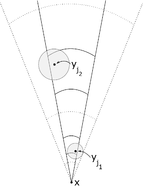
B⁡(yj,c0​2−j)⊂X⁡(x,2​θ0,2−j+1,2−j−2).B(y_{j},c_{0}2^{-j})\subset X(x,2\theta_{0},2^{-j+1},2^{-j-2}).

This is depicted in Figure 1.

Refer to caption
Figure 1. Finding the balls B⁡(yj,c​2−j)⊂X⁡(x,2​θ0,2−j+1,2−j−2)B(y_{j},c2^{-j})\subset X(x,2\theta_{0},2^{-j+1},2^{-j-2}).

Since yj∈Ey_{j}\in E, we infer from (2.4) that

ℋn​(E′∩B⁡(yj,c0​2−j−1))≳2−j​n.\mathcal{H}^{n}(E^{\prime}\cap B(y_{j},c_{0}2^{-j-1}))\gtrsim 2^{-jn}.

Choosing C0=C0​(κ)C_{0}=C_{0}(\kappa) so large that C0≥2/c0C_{0}\geq 2/c_{0} we have that

E′∩B⁡(yj,c0​2−j−1)⊂⋃w∈F′∩B⁡(yj,c0​2−j)B⁡(w,2​δ).E^{\prime}\cap B(y_{j},c_{0}2^{-j-1})\subset\bigcup_{w\in F^{\prime}\cap B(y_{j},c_{0}2^{-j})}B(w,2\delta).

To see this, notice that if u∈E′∩B⁡(yj,c0​2−j−1)u\in E^{\prime}\cap B(y_{j},c_{0}2^{-j-1}), there is w∈F′w\in F^{\prime} so that |w−u|≤δ≤2−j​C0−1≤c0​2−j−1|w-u|\leq\delta\leq 2^{-j}C_{0}^{-1}\leq c_{0}2^{-j-1}. We now conclude that

(2.7) #⁡(F′∩B⁡(yj,c0​2−j))≳δ−n​2−j​n,\#(F^{\prime}\cap B(y_{j},c_{0}2^{-j}))\gtrsim\delta^{-n}2^{-jn},

again by the AD-regularity of E0E_{0}. In order to use Lemma 2.2 we enlarge C0=C0​(κ)C_{0}=C_{0}(\kappa) so that for y∈B⁡(yj,c0​2−j)⊂X⁡(x,2​θ0,2−j+1,2−j−2)y\in B(y_{j},c_{0}2^{-j})\subset X(x,2\theta_{0},2^{-j+1},2^{-j-2}) we have that

|x−y|≥2−j−2≥14​C0​δ≥δmin⁡(δ0,κ/2).|x-y|\geq 2^{-j-2}\geq\frac{1}{4}C_{0}\delta\geq\frac{\delta}{\min(\delta_{0},\kappa/2)}.

Hence, Lemma 2.2 applies to z=x−yz=x-y (since |πℝn​(z)|≤2​θ0​|z|=α0​|z||\pi_{\mathbb{R}^{n}}(z)|\leq 2\theta_{0}|z|=\alpha_{0}|z|), and so

∑y∈F′∩B⁡(yj,c0​2−j)γd,n​(Bx−y∩B⁡(ℝn,κ))≳δ−n​2−j​n​(δ2−j)n=1,\sum_{y\in F^{\prime}\cap B(y_{j},c_{0}2^{-j})}\gamma_{d,n}(B_{x-y}\cap B(\mathbb{R}^{n},\kappa))\gtrsim\delta^{-n}2^{-jn}\Big(\frac{\delta}{2^{-j}}\Big)^{n}=1,

where Bx−y=BzB_{x-y}=B_{z} was defined in Lemma 2.2. Then, varying the scale 2−j2^{-j}, hence the point yjy_{j}, we find ≳M\gtrsim M disjoint balls B⁡(yj,c0​2−j)B(y_{j},c_{0}2^{-j}) inside X⁡(x,2​θ0)X(x,2\theta_{0}) like above, and therefore

∑y∈F′∩X⁡(x,2​θ0)γd,n​(Bx−y∩B⁡(ℝn,κ))≳M.\sum_{y\in F^{\prime}\cap X(x,2\theta_{0})}\gamma_{d,n}(B_{x-y}\cap B(\mathbb{R}^{n},\kappa))\gtrsim M.

This finally yields that

∑x,y∈F′γd,n​(Bx−y∩B⁡(ℝn,κ))\displaystyle\sum_{x,y\in F^{\prime}}\gamma_{d,n}(B_{x-y}\cap B(\mathbb{R}^{n},\kappa)) ≥∑x∈FM∑y∈F′∩X⁡(x,2​θ0)γd,n​(Bx−y∩B⁡(ℝn,κ))\displaystyle\geq\sum_{x\in F^{M}}\sum_{y\in F^{\prime}\cap X(x,2\theta_{0})}\gamma_{d,n}(B_{x-y}\cap B(\mathbb{R}^{n},\kappa))
≳M⋅ℋn​(EM)​δ−n.\displaystyle\gtrsim M\cdot\mathcal{H}^{n}(E^{M})\delta^{-n}.

We then go for the upper bound. For V∈G⁡(d,n)V\in G(d,n) define fV:V→ℝf_{V}\colon V\to\mathbb{R} by setting

fV​(z)=∑x∈F′1B⁡(πV​x,δ)​(z).f_{V}(z)=\sum_{x\in F^{\prime}}1_{B(\pi_{V}x,\delta)}(z).

Notice that

∫VfV​(z)2​d​ℋn​(z)\displaystyle\int_{V}f_{V}(z)^{2}\,d\mathcal{H}^{n}(z) =∑x,y∈F′∫V1B⁡(πV​x,δ)∩B⁡(πV​y,δ)​(z)​d​ℋn​(z)\displaystyle=\sum_{x,y\in F^{\prime}}\int_{V}1_{B(\pi_{V}x,\delta)\cap B(\pi_{V}y,\delta)}(z)\,d\mathcal{H}^{n}(z)
≳δn​#​{(x,y)∈F′×F′:|πV​(x−y)|≤δ}.\displaystyle\gtrsim\delta^{n}\#\{(x,y)\in F^{\prime}\times F^{\prime}\colon\,|\pi_{V}(x-y)|\leq\delta\}.

Therefore, we now have that

ℋn​(EM)​M\displaystyle\mathcal{H}^{n}(E^{M})M ≲δn​∑x,y∈F′γd,n​(Bx−y∩B⁡(ℝn,κ))\displaystyle\lesssim\delta^{n}\sum_{x,y\in F^{\prime}}\gamma_{d,n}(B_{x-y}\cap B(\mathbb{R}^{n},\kappa))
=δn​∫B⁡(ℝn,κ)#⁡{(x,y)∈F′×F′:|πV​(x−y)|≤δ}​d​γd,n​(V)\displaystyle=\delta^{n}\int_{B(\mathbb{R}^{n},\kappa)}\#\{(x,y)\in F^{\prime}\times F^{\prime}\colon\,|\pi_{V}(x-y)|\leq\delta\}\,d\gamma_{d,n}(V)
≲∫B⁡(ℝn,κ)∫VfV​(z)2​d​ℋn​(z)​d​γd,n​(V).\displaystyle\lesssim\int_{B(\mathbb{R}^{n},\kappa)}\int_{V}f_{V}(z)^{2}\,d\mathcal{H}^{n}(z)\,d\gamma_{d,n}(V).

Recall that if x∈F′⊂E′x\in F^{\prime}\subset E^{\prime}, then ℋn​(E1∩B⁡(x,δ))∼δn\mathcal{H}^{n}(E_{1}\cap B(x,\delta))\sim\delta^{n} by (2.3). Using this we estimate fVf_{V} pointwise:

fV​(z)\displaystyle f_{V}(z) ≤δ−n​∑x∈F′|πV​x−z|≤δℋn​(E1∩B⁡(x,δ))\displaystyle\leq\delta^{-n}\mathop{\sum_{x\in F^{\prime}}}_{|\pi_{V}x-z|\leq\delta}\mathcal{H}^{n}(E_{1}\cap B(x,\delta))
≲δ−n​ℋn​(E1∩πV−1​(BV​(z,2​δ)))≲MV​(πV​♯​ℋn|E1)​(z).\displaystyle\lesssim\delta^{-n}\mathcal{H}^{n}(E_{1}\cap\pi_{V}^{-1}(B_{V}(z,2\delta)))\lesssim M_{V}(\pi_{V\sharp}\mathcal{H}^{n}|_{E_{1}})(z).

Here MVM_{V} is the Hardy-Littlewood maximal function on VV. The operator MVM_{V} is bounded on L2​(V)L^{2}(V), see Theorem 1 on p. 13 in Stein’s book [8]. Therefore, we can conclude the proof as follows, using assumption (ii) from Theorem 1.8:

ℋn​(EM)​M≲∫B⁡(ℝn,κ)‖πV​♯​ℋn|E1‖L2​(V)2​d​γd,n​(V)≲1.\mathcal{H}^{n}(E^{M})M\lesssim\int_{B(\mathbb{R}^{n},\kappa)}\|\pi_{V\sharp}\mathcal{H}^{n}|_{E_{1}}\|_{L^{2}(V)}^{2}\,d\gamma_{d,n}(V)\lesssim 1.

∎

3. Proof of the main proposition

Recall the notation for general cones from Definition 1.9. When V=span⁡(w)∈G⁡(d,1)V=\operatorname{span}(w)\in G(d,1), w∈𝕊d−1w\in\mathbb{S}^{d-1}, we introduce shorthand notation for one-dimensional one-sided cones, namely

X+​(x,w,α):=X⁡(x,span⁡(w),α)∩{y∈ℝd:(y−x)⋅w≥0}.X^{+}(x,w,\alpha):=X(x,\operatorname{span}(w),\alpha)\cap\{y\in\mathbb{R}^{d}\colon\,(y-x)\cdot w\geq 0\}.

The restricted version X+​(x,w,α,R,r)X^{+}(x,w,\alpha,R,r), 0<r<R<∞0<r<R<\infty, is defined in the obvious way. We start with a lemma, which states that cones of arbitrary co-dimension with a fixed aperture can be covered by a bounded number of one-dimensional one-sided cones – even ones with a slightly smaller aperture:

Lemma 3.1.

Fix α∈(0,1)\alpha\in(0,1), s∈(0,1]s\in(0,1] and V∈G⁡(d,k)V\in G(d,k). Then, there exist vectors w1,…,wm∈𝕊d−1w_{1},\ldots,w_{m}\in\mathbb{S}^{d-1}, m≲(α​s)1−dm\lesssim(\alpha s)^{1-d}, such that

(3.2) X⁡(0,V,α)⊂⋃j=1mX+​(0,wj,α​s)⊂⋃j=1mX+​(0,wj,α)⊂X⁡(0,V,b​α).X(0,V,\alpha)\subset\bigcup_{j=1}^{m}X^{+}(0,w_{j},\alpha s)\subset\bigcup_{j=1}^{m}X^{+}(0,w_{j},\alpha)\subset X(0,V,b\alpha).

Here b≥1b\geq 1 is a constant depending only on dd.

Proof.

It suffices to find w1,…,wm∈𝕊d−1w_{1},\ldots,w_{m}\in\mathbb{S}^{d-1} such that (3.2) holds with all the cones intersected with 𝕊d−1\mathbb{S}^{d-1}. Find an (α​s)(\alpha s)-net w1,…,wm⊂X⁡(0,V,α)∩𝕊d−1w_{1},\ldots,w_{m}\subset X(0,V,\alpha)\cap\mathbb{S}^{d-1}. Then m≲(α​s)1−dm\lesssim(\alpha s)^{1-d}. Now, write Wj:=wj⟂W_{j}:=w_{j}^{\perp}, fix y∈X⁡(0,V,α)∩𝕊d−1y\in X(0,V,\alpha)\cap\mathbb{S}^{d-1}, and pick wjw_{j} such that |y−wj|≤α​s|y-w_{j}|\leq\alpha s. Then y⋅wj≥0y\cdot w_{j}\geq 0 and

|πWj​(y)|=|πWj​(y−wj)|≤α​s,|\pi_{W_{j}}(y)|=|\pi_{W_{j}}(y-w_{j})|\leq\alpha s,

which proves that y∈X+​(0,wj,α​s)∩𝕊d−1y\in X^{+}(0,w_{j},\alpha s)\cap\mathbb{S}^{d-1} and hence the first inclusion of (3.2). To prove the second inclusion, fix 1≤j≤m1\leq j\leq m and z∈X+​(0,wj,α)∩𝕊d−1z\in X^{+}(0,w_{j},\alpha)\cap\mathbb{S}^{d-1}. Observe that |z−wj|≤b′​α|z-w_{j}|\leq b^{\prime}\alpha for some constant b′=b′​(d)b^{\prime}=b^{\prime}(d), whence

|πV⟂​(z)|≤|πV⟂​(z−wj)|+|πV⟂​(wj)|≤|z−wj|+α≤(b′+1)​α.|\pi_{V^{\perp}}(z)|\leq|\pi_{V^{\perp}}(z-w_{j})|+|\pi_{V^{\perp}}(w_{j})|\leq|z-w_{j}|+\alpha\leq(b^{\prime}+1)\alpha.

This proves the lemma with b=b′+1b=b^{\prime}+1. ∎

Lemma 3.1 allows us to reduce the proof of the main Proposition 1.13 to the "co-dimension 11" case. The relevant (one-dimensional, one-sided) cones in this co-dimension are directed, which is quite useful in the proof.

Proposition 3.3 (Main proposition in co-dimension 11).

Let w∈𝕊d−1w\in\mathbb{S}^{d-1}. Assume that an ℋn\mathcal{H}^{n}-measurable set F⊂ℝdF\subset\mathbb{R}^{d} satisfies the following conditions:

  • (a)

    ℋn​(F)=:τ>0\mathcal{H}^{n}(F)=:\tau>0, and F⊂E0∩B⁡(0,1)F\subset E_{0}\cap B(0,1) for some nn-ADR set E0E_{0},

  • (b)

    for some α>0\alpha>0, M∈ℕM\in\mathbb{N}, and for every point x∈Fx\in F there holds that

    #⁡{j∈ℤ:X+​(x,w,α,2−j,2−j−1)∩F≠∅}≤M.\#\{j\in\mathbb{Z}\colon\,X^{+}(x,w,\alpha,2^{-j},2^{-j-1})\cap F\neq\emptyset\}\leq M.

We abbreviate (a) and (b) by saying that that FF satisfies the (α,M,w)(\alpha,M,w)-property. Then, if M≥1M\geq 1 and α>0\alpha>0 is small enough (depending on only on dd), there exists a compact set K⊂FK\subset F with ℋn(K)∼τ,α1\mathcal{H}^{n}(K)\sim_{\tau,\alpha}1, which satisfies the (α/2,M−1,w)(\alpha/2,M-1,w)-property.

The general idea of the argument is to write down an explicit algorithm, which refines FF by deleting some points in several stages, but all the time keeps track that not too much is wasted. When the algorithm eventually stops, it will output the desired set KK. Before giving the details, let us see how the general version of the main proposition follows from Proposition 3.3.

Proof of Proposition 1.13.

Assume that E2⊂E0E_{2}\subset E_{0} satisfies the nn-dimensional (θ0,M0)(\theta_{0},M_{0})-property. Then, with V=(ℝn)⟂V=(\mathbb{R}^{n})^{\perp},

#⁡{j∈ℤ:X⁡(x,V,θ0,2−j,2−j−1)∩E2≠∅}≤M0\#\{j\in\mathbb{Z}:X(x,V,\theta_{0},2^{-j},2^{-j-1})\cap E_{2}\neq\emptyset\}\leq M_{0}

for all x∈E2x\in E_{2}. Now, use Lemma 3.1 with α=θ0/b\alpha=\theta_{0}/b and s=2−M0s=2^{-M_{0}} to find vectors w1,…,wm∈𝕊1w_{1},\ldots,w_{m}\in\mathbb{S}^{1}, m≲(θ0/(2M0​b))1−dm\lesssim(\theta_{0}/(2^{M_{0}}b))^{1-d}, such that

X⁡(0,V,θ0/b)⊂⋃j=1mX+​(0,wj,θ0/(2M0​b))⊂⋃j=1mX+​(0,wj,θ0/b)⊂X⁡(0,V,θ0).X(0,V,\theta_{0}/b)\subset\bigcup_{j=1}^{m}X^{+}(0,w_{j},\theta_{0}/(2^{M_{0}}b))\subset\bigcup_{j=1}^{m}X^{+}(0,w_{j},\theta_{0}/b)\subset X(0,V,\theta_{0}).

It follows from translation invariance that

(3.4) X⁡(x,V,θ0/b,2−j,2−j−1)⊂⋃j=1mX+​(x,wj,θ0/(2M0​b),2−j,2−j−1)X(x,V,\theta_{0}/b,2^{-j},2^{-j-1})\subset\bigcup_{j=1}^{m}X^{+}(x,w_{j},\theta_{0}/(2^{M_{0}}b),2^{-j},2^{-j-1})

for all x∈ℝdx\in\mathbb{R}^{d} and j∈ℤj\in\mathbb{Z}. Further, E2E_{2} satisfies the (θ0/b,M0,wj)(\theta_{0}/b,M_{0},w_{j})-property from Proposition 3.3 for all 1≤j≤m1\leq j\leq m. Thus, iterating that proposition ≤M0\leq M_{0} times for each 1≤j≤m1\leq j\leq m, hence ≤m​M0\leq mM_{0} times altogether, one finds a set E3⊂E2E_{3}\subset E_{2} satisfying the (θ0/(2M0​b),0,wj)(\theta_{0}/(2^{M_{0}}b),0,w_{j})-property for all 1≤j≤m1\leq j\leq m. It follows from (3.4) that E3E_{3} satisfies the nn-dimensional (θ0/b,0)(\theta_{0}/b,0)-property, and Proposition 1.13 is proved. ∎

Proof of Proposition 3.3.

We assume that w=ed=(0,0,…,0,1)w=e_{d}=(0,0,\ldots,0,1). Before starting to describe the algorithm to find K⊂FK\subset F, we make two easy reductions: first, without loss of generality, we may assume that if x∈Fx\in F and

X+​(x,w,α,2−j,2−j−1)∩F≠∅X^{+}(x,w,\alpha,2^{-j},2^{-j-1})\cap F\neq\emptyset

then 2−j≥δ2^{-j}\geq\delta for some small constant δ>0\delta>0. Simply, for every x∈Fx\in F, there is some δx>0\delta_{x}>0 with this property, and then we can take δ>0\delta>0 so small that ℋn​(F′)≥ℋn​(F)/2\mathcal{H}^{n}(F^{\prime})\geq\mathcal{H}^{n}(F)/2, where F′:=F∖{x∈F:δx<δ}F^{\prime}:=F\setminus\{x\in F:\delta_{x}<\delta\}. After this, we would proceed with the proof as below, only replacing FF by F′F^{\prime}. Second, we may assume that FF is compact; otherwise we can always find a compact subset of FF (or F′F^{\prime}) with almost the same ℋn\mathcal{H}^{n}-measure, and then we can find KK inside this subset as below.

We now begin to describe the algorithm. The following points (I)–(IV) summarise the key features.

  • (I)

    There will be a sequence of compact sets F=F0⊃F1⊃F2⊃⋯F=F^{0}\supset F^{1}\supset F^{2}\supset\cdots, where Fk+1F^{k+1} is obtained from FkF^{k} by deleting a certain open set DkD^{k}.

  • (II)

    Thus, there will also be a sequence of deleted sets Dk⊂FkD^{k}\subset F^{k}, k∈{0,1,…}k\in\{0,1,\ldots\}.

  • (III)

    There will be a sequence of saved sets Sk⊂Fk⊂FS^{k}\subset F^{k}\subset F, k={0,1,…}k=\{0,1,\ldots\}, which are disjoint from each other and all the deleted sets DiD^{i}, i≥ki\geq k,11 1 The sets SkS^{k} are also disjoint from the deleted sets DiD^{i} with i<ki<k, as Sk⊂Fk=F∖⋃i<kDiS^{k}\subset F^{k}=F\setminus\bigcup_{i<k}D^{i}. satisfy

    ℋn​(Sk)≳max⁡{ℋn​(Dk),δn},\mathcal{H}^{n}(S^{k})\gtrsim\max\{\mathcal{H}^{n}(D^{k}),\delta^{n}\},

    and have the property that if

    x∈⋃i≤kSi,x\in\bigcup_{i\leq k}S^{i},

    then there are at most M−1M-1 scales 2−j2^{-j} such that

    X+​(x,w,α/2,2−j,2−j−1)∩⋃i≤kSi≠∅.X^{+}(x,w,\alpha/2,2^{-j},2^{-j-1})\cap\bigcup_{i\leq k}S^{i}\neq\emptyset.
  • (IV)

    We describe the structure of the saved sets. Let Fk,MF^{k,M} be the set of points in FkF^{k} such that there are exactly MM scales 2−j≥δ2^{-j}\geq\delta such that

    X+​(x,w,α/2,2−j,2−j−1)∩Fk≠∅.X^{+}(x,w,\alpha/2,2^{-j},2^{-j-1})\cap F^{k}\neq\emptyset.

    A point x∈Fkx\in F^{k} is then called kk-bad, if x∈Fk,Mx\in F^{k,M}, and furthermore

    ℋn​(B⁡(x,r)∩Fk,M)≥ϵ​rn\mathcal{H}^{n}(B(x,r)\cap F^{k,M})\geq\epsilon r^{n}

    for all radii 0<r≤10<r\leq 1, where ϵ∼ℋn​(F)\epsilon\sim\mathcal{H}^{n}(F) is a constant to be specified in Stopping condition 3.6 below. Using the compactness of FkF^{k} and the uniform lower bound for the numbers 2−j2^{-j}, it is easy to verify that the set of kk-bad points is compact. Thus, if there are any kk-bad points to begin with, there exists a (possibly non-unique) kk-bad point xkx_{k} with the smallest last coordinate xkdx_{k}^{d}. With such a choice of xkx_{k}, the saved set SkS^{k} will be defined as B⁡(xk,rk)∩Fk,MB(x_{k},r_{k})\cap F^{k,M} for some suitable radius rk≳δr_{k}\gtrsim\delta.

    Note that if xx is kk-bad and k≥1k\geq 1, then xx is also (k−1)(k-1)-bad, simply because Fk⊂Fk−1F^{k}\subset F^{k-1} and Fk,M⊂Fk−1,MF^{k,M}\subset F^{k-1,M}. This implies, by the definition of xkx_{k}, that the last coordinates of the points x0,x1,…,xkx_{0},x_{1},\ldots,x_{k} form a non-decreasing sequence.

    Finally, to every set Sk=B⁡(xk,rk)∩Fk,MS^{k}=B(x_{k},r_{k})\cap F^{k,M} we associate a somewhat larger set Bk:=B⁡(xk,100​rk)∩FkB^{k}:=B(x_{k},100r_{k})\cap F^{k}, which will have the property that if x∈Bkx\in B^{k}, then there are at most M−1M-1 scales 2−j2^{-j} such that

    X+​(x,w,α/2,2−j,2−j−1)∩Fk+1≠∅.X^{+}(x,w,\alpha/2,2^{-j},2^{-j-1})\cap F^{k+1}\neq\emptyset.

There will be two different stopping conditions, which bring the algorithm to a halt and output the desired set KK.

Stopping condition 3.5.

Assume that the sets D0,…,DkD^{0},\ldots,D^{k} and S0,…,SkS^{0},\ldots,S^{k} have been defined, and either

∑i=0kℋn​(Di)≥ℋn​(F)/2\sum_{i=0}^{k}\mathcal{H}^{n}(D^{i})\geq\mathcal{H}^{n}(F)/2

or

∑i=0kℋn​(Si)≥ℋn​(F)/2.\sum_{i=0}^{k}\mathcal{H}^{n}(S^{i})\geq\mathcal{H}^{n}(F)/2.

In both cases, we set

K:=⋃i≤kSi.K:=\bigcup_{i\leq k}S^{i}.

By (III), the set KK satisfies the requirements of Proposition 3.3, and the proof is complete.

Stopping condition 3.6.

Assume that the set FkF^{k} has been defined, and satisfies ℋn​(Fk)≥ℋn​(F)/2\mathcal{H}^{n}(F^{k})\geq\mathcal{H}^{n}(F)/2, and that the set of kk-bad points, as in (IV), is empty. Thus, for every x∈Fk,Mx\in F^{k,M}, we have

ℋn​(Fk,M∩B⁡(x,rx))≤ϵ​rxn\mathcal{H}^{n}(F^{k,M}\cap B(x,r_{x}))\leq\epsilon r_{x}^{n}

for some radius 0<rx≤10<r_{x}\leq 1. Now choose ϵ∼ℋn​(F)∼1\epsilon\sim\mathcal{H}^{n}(F)\sim 1 so small that, using Lemma 2.1, we have ℋn​(Fk,M)≤ℋn​(F)/4\mathcal{H}^{n}(F^{k,M})\leq\mathcal{H}^{n}(F)/4. We set

K:=Fk∖Fk,M.K:=F^{k}\setminus F^{k,M}.

Then, ℋn​(K)≥ℋn​(Fk)−ℋn​(Fk,M)≥ℋn​(F)/4\mathcal{H}^{n}(K)\geq\mathcal{H}^{n}(F^{k})-\mathcal{H}^{n}(F^{k,M})\geq\mathcal{H}^{n}(F)/4, and for every x∈Kx\in K there are at most M−1M-1 scales 2−j2^{-j} such that

X+​(x,w,α/2,2−j,2−j−1)∩K≠∅.X^{+}(x,w,\alpha/2,2^{-j},2^{-j-1})\cap K\neq\emptyset.

Thus, KK satisfies the requirements of Proposition 3.3, and the proof is complete.

Remark 3.7.

Notice that, since ℋn​(Sk)≳δn\mathcal{H}^{n}(S^{k})\gtrsim\delta^{n} for every kk, the first stopping condition will be reached in ≲δ−n\lesssim\delta^{-n} steps (unless the second stopping condition was reached before that). In particular, the algorithm terminates and outputs KK after finitely many steps.

Next, we will explicitly describe how to construct the various sets FkF^{k}, SkS^{k} and DkD^{k}. Define S−1=∅S^{-1}=\emptyset, D−1=∅D^{-1}=\emptyset and F0:=FF^{0}:=F. Assume that k≥0k\geq 0 and the sets F0,…,FkF^{0},\ldots,F^{k}, D1,…,Dk−1D^{1},\ldots,D^{k-1} and S1,…,Sk−1S^{1},\ldots,S^{k-1} have already been defined, and satisfy the properties listed in (I)–(IV); in particular, also the balls BiB^{i}, i<ki<k, have been defined. Assume that the first stopping condition is not satisfied; otherwise the algorithm terminates and the proof is complete. In particular,

(3.8) ℋn​(Fk)≥ℋn​(F)−∑i<kℋn​(Di)≥ℋn​(F)/2.\mathcal{H}^{n}(F^{k})\geq\mathcal{H}^{n}(F)-\sum_{i<k}\mathcal{H}^{n}(D^{i})\geq\mathcal{H}^{n}(F)/2.

Next, assume that the second stopping condition is not satisfied; because of (3.8), this means that the set of kk-bad points is non-empty, and – as required by (IV) – we find one of them, xkx_{k}, with minimal last coordinate. Let 2−jk2^{-j_{k}} be one of the MM scales such that

(3.9) X+​(xk,w,α/2,2−jk,2−jk−1)∩Fk≠∅.X^{+}(x_{k},w,\alpha/2,2^{-j_{k}},2^{-j_{k}-1})\cap F^{k}\neq\emptyset.

Let rk:=c​2−jkr_{k}:=c2^{-j_{k}} for a suitable small c=c⁡(d,α)>0c=c(d,\alpha)>0 to be specified later, and set

Sk:=B⁡(xk,rk)∩Fk,M,Bk:=B⁡(xk,100​rk)∩Fk,S^{k}:=B(x_{k},r_{k})\cap F^{k,M},\qquad B^{k}:=B(x_{k},100r_{k})\cap F^{k},

as required by (IV). Then

(3.10) ℋn​(Sk)≳2−jk​n≥δn,\mathcal{H}^{n}(S^{k})\gtrsim 2^{-j_{k}n}\geq\delta^{n},

by the definition of kk-badness. Furthermore, SkS^{k} is disjoint from all the previous sets SiS^{i}, i<ki<k, and even the larger sets BiB^{i}, i<ki<k, because Sk⊂Fk,MS^{k}\subset F^{k,M}, but if x∈Bix\in B^{i}, then

(3.11) X+​(x,w,α/2,2−m,2−m−1)∩Fk≠∅X^{+}(x,w,\alpha/2,2^{-m},2^{-m-1})\cap F^{k}\neq\emptyset

can only hold for M−1M-1 scales 2−m2^{-m} by (IV). Next, we define the deleted set DkD^{k} by

Dk:=Fk∩⋃l∈{−1,0,1}⋃x∈BkX∘​(x,w,α,2−jk+l,2−jk−1+l).D^{k}:=F^{k}\cap\bigcup_{l\in\{-1,0,1\}}\bigcup_{x\in B^{k}}X^{\circ}(x,w,\alpha,2^{-j_{k}+l},2^{-j_{k}-1+l}).

Here X∘X^{\circ} stands for the interior of the cone X+X^{+} (we want the deleted set to be relatively open in FkF^{k}). Then DkD^{k} is contained in a single ball of radius ≲2−jk\lesssim 2^{-j_{k}}, so ℋn​(Dk)≲2−jk​n\mathcal{H}^{n}(D^{k})\lesssim 2^{-j_{k}n}. Combining this with (3.10), we see that

ℋn​(Sk)≳max⁡{ℋn​(Dk),δn},\mathcal{H}^{n}(S^{k})\gtrsim\max\{\mathcal{H}^{n}(D^{k}),\delta^{n}\},

as required in (III).

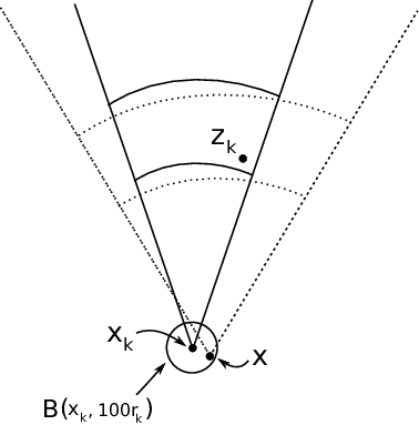
To complete the proof, we still need to show the disjointness of DkD_{k} from the previous saved sets SiS^{i}, i<ki<k, the latter claim in (III) about ⋃i≤kSi\bigcup_{i\leq k}S^{i}, and the claim about the set BkB^{k} at the end of (IV). We begin with the last and easiest task. By the definition of 2−jk2^{-j_{k}} in (3.9), there exists a point

zk∈X+​(xk,w,α/2,2−jk,2−jk−1)∩Fk.z_{k}\in X^{+}(x_{k},w,\alpha/2,2^{-j_{k}},2^{-j_{k}-1})\cap F^{k}.

Now, if the constant cc in rk=c​2−jkr_{k}=c2^{-j_{k}} is chosen small enough (depending on α\alpha), and x∈Bk⊂B⁡(xk,100​rk)x\in B^{k}\subset B(x_{k},100r_{k}), one can check that

zk∈⋃l∈{−1,0,1}X+​(x,w,α,2−jk+l,2−jk−1+l),z_{k}\in\bigcup_{l\in\{-1,0,1\}}X^{+}(x,w,\alpha,2^{-j_{k}+l},2^{-j_{k}-1+l}),
Refer to caption
Figure 2. Some of the points and regions associated with DkD^{k}.

see Figure 2. In particular, one of the three scales 2−jk+l2^{-j_{k}+l}, l∈{−1,0,1}l\in\{-1,0,1\}, is among the at most MM scales 2−m2^{-m} such that X+​(x,w,α,2−m,2−m−1)∩Fk≠∅X^{+}(x,w,\alpha,2^{-m},2^{-m-1})\cap F^{k}\neq\emptyset. Then DkD^{k} certainly contains all the points in the intersection X+​(x,w,α/2,2−m,2−m−1)∩FkX^{+}(x,w,\alpha/2,2^{-m},2^{-m-1})\cap F^{k}, so

X+​(x,w,α/2,2−m,2−m−1)∩Fk+1=X+​(x,w,α/2,2−m,2−m−1)∩(Fk∖Dk)=∅.X^{+}(x,w,\alpha/2,2^{-m},2^{-m-1})\cap F^{k+1}=X^{+}(x,w,\alpha/2,2^{-m},2^{-m-1})\cap(F^{k}\setminus D^{k})=\emptyset.

Thus, there can only remain at most M−1M-1 scales 2−m2^{-m} such that

(3.12) X+​(x,w,α/2,2−m,2−m−1)∩Fk+1≠∅,x∈Bk,X^{+}(x,w,\alpha/2,2^{-m},2^{-m-1})\cap F^{k+1}\neq\emptyset,\quad x\in B^{k},

and this is exactly what is claimed at the end of (IV).

Finally, we establish the remaining claims in (III) by proving that DkD^{k} is disjoint from the saved sets SiS^{i}, i≤ki\leq k. In fact, this implies that Si∩Dl=∅S^{i}\cap D^{l}=\emptyset for all pairs i,l≤ki,l\leq k. Indeed, if i≤l<ki\leq l<k, we may assume by induction that SiS^{i} is disjoint from DlD^{l} (since this is precisely what we are about to prove for l=kl=k). Further, SiS^{i} is disjoint from DlD^{l} with l<il<i simply because

Si⊂Fi=F∖⋃l<iDl.S^{i}\subset F^{i}=F\setminus\bigcup_{l<i}D^{l}.

From the previous discussion, we conclude that

(3.13) ⋃i≤kSi⊂F∖⋃l≤kDl=Fk+1.\bigcup_{i\leq k}S^{i}\subset F\setminus\bigcup_{l\leq k}D^{l}=F^{k+1}.

Observe that for every x∈⋃i≤kSix\in\bigcup_{i\leq k}S^{i} there are at most M−1M-1 scales 2−j2^{-j} such that

X+​(x,w,α/2,2−j,2−j−1)∩Fk+1≠∅.X^{+}(x,w,\alpha/2,2^{-j},2^{-j-1})\cap F^{k+1}\neq\emptyset.

This follows from (3.12) for x∈Sk⊂Bkx\in S^{k}\subset B^{k}, and from induction for x∈Si⊂Bix\in S^{i}\subset B^{i} for i<ki<k (recalling (3.11) and noting that Fk+1⊂FkF_{k+1}\subset F_{k}). Hence, we infer from the inclusion (3.13) that there are also at most M−1M-1 scales 2−j2^{-j} such that

X+​(x,w,α/2,2−j,2−j−1)∩⋃i≤kSi≠∅X^{+}(x,w,\alpha/2,2^{-j},2^{-j-1})\cap\bigcup_{i\leq k}S^{i}\neq\emptyset

for x∈⋃i≤kSix\in\bigcup_{i\leq k}S^{i}. This is what was claimed at the end of (III).
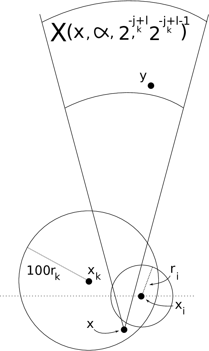
Refer to caption
Figure 3. The case 100​rk≤ri100r_{k}\leq r_{i}.

Now, we fix i≤ki\leq k, and establish that DkD^{k} is disjoint from SiS^{i}. If i=ki=k, this is immediate from the construction (recall that Sk⊂B⁡(xk,rk)S^{k}\subset B(x_{k},r_{k}), whereas DkD^{k} lies inside the union of certain annuli, all at distance ≫rk\gg r_{k} from xkx_{k}). So, we assume that i<ki<k. There are two cases to consider. First, assume that 100​rk≤ri100r_{k}\leq r_{i} (see Figure 3). In this case, we simply prove that if x∈Bk⊂B⁡(xk,100​rk)⊂B⁡(xk,ri)x\in B^{k}\subset B(x_{k},100r_{k})\subset B(x_{k},r_{i}), then

(3.14) X+​(x,w,α)∩B⁡(xi,ri)=∅,X^{+}(x,w,\alpha)\cap B(x_{i},r_{i})=\emptyset,

which is clearly a stronger statement than Dk∩Si=∅D^{k}\cap S^{i}=\emptyset. Fix x∈Bkx\in B^{k}, and recall that xk∉Bi=B⁡(xi,100​ri)∩Fix_{k}\notin B^{i}=B(x_{i},100r_{i})\cap F^{i} for i<ki<k (because xk∈Skx_{k}\in S_{k}, and SkS_{k} is disjoint from BiB^{i}, as remarked below (3.10)). Because xk∈Sk⊂Fk⊂Fix_{k}\in S^{k}\subset F^{k}\subset F^{i}, this implies that xk∉B⁡(xi,100​ri)x_{k}\notin B(x_{i},100r_{i}), and hence, by 100​rk≤ri100r_{k}\leq r_{i},

(3.15) x∉B⁡(xi,50​ri).x\notin B(x_{i},50r_{i}).

Now, recall that the last coordinate of xkx_{k} is no smaller than the last coordinate of xix_{i} by (IV). So, if we write y=(yu)u=1dy=(y^{u})_{u=1}^{d} for a general point y∈ℝdy\in\mathbb{R}^{d}, we have

(3.16) xd≥xkd−ri≥xid−ri.x^{d}\geq x_{k}^{d}-r_{i}\geq x_{i}^{d}-r_{i}.

It is now easy to check, based on (3.15) and (3.16) that (3.14) holds, if we assume that, say, α≤1/10\alpha\leq 1/10.

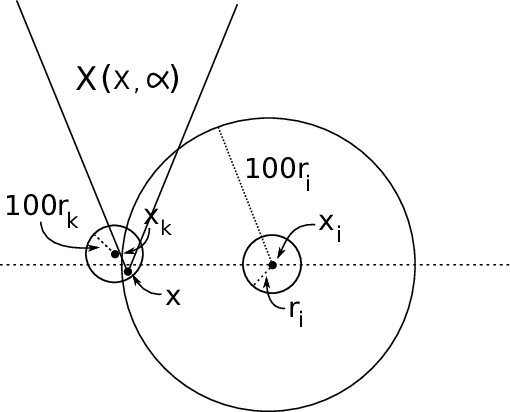
Refer to caption
Figure 4. The case 100​rk>ri100r_{k}>r_{i}.

Next, assume that 100​rk>ri100r_{k}>r_{i} (see Figure 4). Recall that rk=c​2−jkr_{k}=c2^{-j_{k}}, and DkD^{k} is contained in the union of the annuli X∘​(x,w,α,2−jk+l,2−jk−1+l)X^{\circ}(x,w,\alpha,2^{-j_{k}+l},2^{-j_{k}-1+l}), where x∈Bk⊂B⁡(xk,100​rk)x\in B^{k}\subset B(x_{k},100r_{k}) and l∈{−1,0,1}l\in\{-1,0,1\}. If x∈Bkx\in B^{k} is fixed, then by the same argument that gave (3.16), we now have

(3.17) xd≥xkd−100​rk≥xid−100​c​2−jk.x^{d}\geq x_{k}^{d}-100r_{k}\geq x_{i}^{d}-100c2^{-j_{k}}.

If

y∈X∘​(x,w,α,2−jk+l,2−jk−1+l),y\in X^{\circ}(x,w,\alpha,2^{-j_{k}+l},2^{-j_{k}-1+l}),

then, using (3.17) and choosing c>0c>0 small enough,

yd≥xd+2−jk−10≥xid+2−jk−20≥xid+1000​c​2−jk≥xid+10​ri.y^{d}\geq x^{d}+2^{-j_{k}-10}\geq x_{i}^{d}+2^{-j_{k}-20}\geq x_{i}^{d}+1000c2^{-j_{k}}\geq x_{i}^{d}+10r_{i}.

In particular, yy cannot lie in B⁡(xi,ri)⊃SiB(x_{i},r_{i})\supset S^{i}, and the proof is complete. ∎

Appendix A A measure estimate on the Grassmannian

This section contains the proof of Lemma 2.2. Let us recall the statement:

Lemma A.1.

Fix υ,δ>0\upsilon,\delta>0 and let W∈G⁡(d,n)W\in G(d,n). Assume that z∈ℝdz\in\mathbb{R}^{d} satisfies δ/|z|<min⁡(δ0,υ/2)\delta/|z|<\min(\delta_{0},\upsilon/2), where δ0\delta_{0} is a small constant depending only on dd, and |πW​z|≤α0​|z||\pi_{W}z|\leq\alpha_{0}|z| for a small enough α0=α0​(n,υ)>0\alpha_{0}=\alpha_{0}(n,\upsilon)>0. Define Bz={V∈G⁡(d,n):|πV​z|≤δ}B_{z}=\{V\in G(d,n)\colon\,|\pi_{V}z|\leq\delta\}. Then,

A(z):=γd,n(Bz∩BG⁡(d,n)(W,υ))≳υ(δ|z|)n.A(z):=\gamma_{d,n}(B_{z}\cap B_{G(d,n)}(W,\upsilon))\gtrsim_{\upsilon}\Big(\frac{\delta}{|z|}\Big)^{n}.
Proof.

Let us begin by showing that there exists V0∈BG⁡(d,n)​(W,υ/2)V_{0}\in B_{G(d,n)}(W,\upsilon/2) for which πV0​z=0\pi_{V_{0}}z=0. Let e1,…,en∈ℝde_{1},\ldots,e_{n}\in\mathbb{R}^{d} be an orthonormal basis for WW. Notice that for every j∈{1,…,n}j\in\{1,\ldots,n\} we have that

|z⋅ej|≤|πW​z|≤α0​|z|.|z\cdot e_{j}|\leq|\pi_{W}z|\leq\alpha_{0}|z|.

The plan is now to form new vectors u1,…,unu_{1},\ldots,u_{n} by perturbing the vectors e1,…,ene_{1},\ldots,e_{n} slightly. Let u0:=e0:=z/|z|u_{0}:=e_{0}:=z/|z|, Z−1:=∅Z_{-1}:=\emptyset and ϵ0:=α0\epsilon_{0}:=\alpha_{0}. Assume that u0,…,uku_{0},\ldots,u_{k}, 0≤k<n0\leq k<n, have already been defined so that they satisfy:

  1. (1)

    (u0,u1,…,uk)(u_{0},u_{1},\ldots,u_{k}) is an orthonormal sequence;

  2. (2)

    If Zi=span​(u0,u1,…,ui)Z_{i}=\textup{span}(u_{0},u_{1},\ldots,u_{i}) for i∈{0,…,k}i\in\{0,\ldots,k\} then

    ui=πZi−1⟂​ei|πZi−1⟂​ei|u_{i}=\frac{\pi_{Z_{i-1}^{\perp}}e_{i}}{|\pi_{Z_{i-1}^{\perp}}e_{i}|}

    and

    (A.2) |πZi​ei+1|≤ϵi.|\pi_{Z_{i}}e_{i+1}|\leq\epsilon_{i}.

As will be apparent in a moment, the numbers ϵi\epsilon_{i} will be defined via a simple recurrence relation. Observe that (A.2) also gives

|πZi⟂​ei+1|≥(1−ϵi2)1/2,i∈{0,…,k}.|\pi_{Z_{i}^{\perp}}e_{i+1}|\geq(1-\epsilon_{i}^{2})^{1/2},\qquad i\in\{0,\ldots,k\}.

Now, let

uk+1=πZk⟂​ek+1|πZk⟂​ek+1|u_{k+1}=\frac{\pi_{Z_{k}^{\perp}}e_{k+1}}{|\pi_{Z_{k}^{\perp}}e_{k+1}|}

and Zk+1=span​(Zk,uk+1)Z_{k+1}=\textup{span}(Z_{k},u_{k+1}). If k=n−1k=n-1, the vectors {u1,…,un}\{u_{1},\ldots,u_{n}\} have now been defined, and the induction terminates. If k<n−1k<n-1, notice that

|πZk+1​ek+2|2\displaystyle|\pi_{Z_{k+1}}e_{k+2}|^{2} =∑i=0k+1(ek+2⋅ui)2\displaystyle=\sum_{i=0}^{k+1}(e_{k+2}\cdot u_{i})^{2}
=(ek+2⋅u0)2+∑i=1k+1(ek+2⋅πZi−1⟂​ei|πZi−1⟂​ei|)2\displaystyle=(e_{k+2}\cdot u_{0})^{2}+\sum_{i=1}^{k+1}\Big(e_{k+2}\cdot\frac{\pi_{Z_{i-1}^{\perp}}e_{i}}{|\pi_{Z_{i-1}^{\perp}}e_{i}|}\Big)^{2}
=(ek+2⋅u0)2+∑i=1k+1(ek+2⋅πZi−1​ei|πZi−1⟂​ei|)2\displaystyle=(e_{k+2}\cdot u_{0})^{2}+\sum_{i=1}^{k+1}\Big(e_{k+2}\cdot\frac{\pi_{Z_{i-1}}e_{i}}{|\pi_{Z_{i-1}^{\perp}}e_{i}|}\Big)^{2}
≤α02+∑i=1k+1ϵi−121−ϵi−12=:ϵk+12.\displaystyle\leq\alpha_{0}^{2}+\sum_{i=1}^{k+1}\frac{\epsilon_{i-1}^{2}}{1-\epsilon_{i-1}^{2}}=:\epsilon_{k+1}^{2}.

Now, properties (1) and (2) have been verified for the vectors u0,…,uk+1u_{0},\ldots,u_{k+1}.

Define V0=span​(u1,…,un)V_{0}=\textup{span}(u_{1},\ldots,u_{n}). By (1) it follows that πV0​z=0\pi_{V_{0}}z=0. Therefore, it remains to show that V0∈BG⁡(d,n)​(W,υ/2)V_{0}\in B_{G(d,n)}(W,\upsilon/2) for a small enough α0\alpha_{0}. First, it is easy to check using the definition of uiu_{i} that

ui−ei\displaystyle u_{i}-e_{i} =−πZi−1​ei|πZi−1⟂​ei|+(1|πZi−1⟂​ei|−1)​ei.\displaystyle=\frac{-\pi_{Z_{i-1}}e_{i}}{|\pi_{Z_{i-1}^{\perp}}e_{i}|}+\Big(\frac{1}{|\pi_{Z_{i-1}^{\perp}}e_{i}|}-1\Big)e_{i}.

It follows that

|ui−ei|≤ϵi−1(1−ϵi−12)1/2+(1(1−ϵi−12)1/2−1)=:ri.|u_{i}-e_{i}|\leq\frac{\epsilon_{i-1}}{(1-\epsilon_{i-1}^{2})^{1/2}}+\Big(\frac{1}{(1-\epsilon_{i-1}^{2})^{1/2}}-1\Big)=:r_{i}.

Choose α0\alpha_{0} so small that max{ri:i=1,…,n}≤υ/(4n1/2)\max\{r_{i}\colon i=1,\ldots,n\}\leq\upsilon/(4n^{1/2}); this can clearly be done, given that the numbers ϵi\epsilon_{i} satisfy the recurrence relation above. It follows that

‖W−V0‖G⁡(d,n)=‖πW−πV0‖≤υ/4,\|W-V_{0}\|_{G(d,n)}=\|\pi_{W}-\pi_{V_{0}}\|\leq\upsilon/4,

ending the proof of the existence of V0V_{0}.

Let F={V∈G⁡(d,n):πV​z=0}F=\{V\in G(d,n)\colon\pi_{V}z=0\} and identify FF with G⁡(d−1,n)G(d-1,n) (notice that FF is exactly the nn-planes contained in z⟂≈ℝd−1z^{\perp}\approx\mathbb{R}^{d-1}). Now V0∈FV_{0}\in F. Let HH be a maximal δ/|z|\delta/|z|-separated collection of V∈BG⁡(d−1,n)​(V0,υ/2)V\in B_{G(d-1,n)}(V_{0},\upsilon/2). Then BG⁡(d−1,n)​(V0,υ/2)⊂⋃{BG⁡(d−1,n)​(V,2​δ/|z|):V∈H}B_{G(d-1,n)}(V_{0},\upsilon/2)\subset\bigcup\{B_{G(d-1,n)}(V,2\delta/|z|)\colon\,V\in H\} yielding that

1≲υ#H⋅(δ|z|)n⁡(d−1−n).1\lesssim_{\upsilon}\#H\cdot\Big(\frac{\delta}{|z|}\Big)^{n(d-1-n)}.

Here we used that γd−1,n(BG⁡(d−1,n)(V0,υ/2))∼υ1\gamma_{d-1,n}(B_{G(d-1,n)}(V_{0},\upsilon/2))\sim_{\upsilon}1 and Proposition 4.1 of [5] (we also implicitly used δ/|z|<δ0\delta/|z|<\delta_{0}, which, for small enough δ0\delta_{0}, guarantees that Proposition 4.1 of [5] applies to the balls BG⁡(d−1,n)​(V,2​δ/|z|)B_{G(d-1,n)}(V,2\delta/|z|)). Notice that

⋃V∈HBG⁡(d,n)​(V,δ/(2​|z|))⊂Bz∩BG⁡(d,n)​(W,υ)\bigcup_{V\in H}B_{G(d,n)}(V,\delta/(2|z|))\subset B_{z}\cap B_{G(d,n)}(W,\upsilon)

by the definition of BzB_{z}, the inclusion H⊂FH\subset F, and the inequalities δ/(2​|z|)≤υ/4\delta/(2|z|)\leq\upsilon/4, and

‖V−W‖G⁡(d,n)≤‖V−V0‖G⁡(d−1,n)+‖V0−W‖G⁡(d,n)≤3​υ4,V∈H.\|V-W\|_{G(d,n)}\leq\|V-V_{0}\|_{G(d-1,n)}+\|V_{0}-W\|_{G(d,n)}\leq\frac{3\upsilon}{4},\qquad V\in H.

Also, the G⁡(d,n)G(d,n)-balls in the union are disjoint, so

A(z)≥∑V∈Hγd,n(BG⁡(d,n)(V,δ/(2|z|)))≳υ(δ|z|)n⁡(d−n)⋅(δ|z|)−n⁡(d−1−n)=(δ|z|)n,A(z)\geq\sum_{V\in H}\gamma_{d,n}(B_{G(d,n)}(V,\delta/(2|z|)))\gtrsim_{\upsilon}\Big(\frac{\delta}{|z|}\Big)^{n(d-n)}\cdot\Big(\frac{\delta}{|z|}\Big)^{-n(d-1-n)}=\Big(\frac{\delta}{|z|}\Big)^{n},

using the cardinality estimate for HH, and Proposition 4.1 of [5] again. ∎

References

  • [1] J. Azzam and R. Schul (2012) Hard sard: quantitative implicit function and extension theorems for lipschitz maps. Geom. Funct. Anal. 22 (5), pp. 1062–1123. Cited by: §1.
  • [2] G. David and S. Semmes (1991) Singular integrals and rectifiable sets in 𝐑n{\bf R}^{n}: beyond lipschitz graphs. Astérisque (193), pp. 152. External Links: ISSN 0303-1179 Cited by: §1.
  • [3] G. David and S. Semmes (1993) Analysis of and on uniformly rectifiable sets. Mathematical Surveys and Monographs, Vol. 38, American Mathematical Society, Providence, RI. Cited by: §1, §1.
  • [4] G. David and S. Semmes (1993) Quantitative rectifiability and lipschitz mappings. Trans. Amer. Math. Soc. 337 (2), pp. 855–889. External Links: ISSN 0002-9947 Cited by: §1, §1.
  • [5] K. Fässler and T. Orponen (2013) Constancy results for special families of projections. Math. Proc. Cambridge Philos. Soc. 154 (3), pp. 549–568. Cited by: Appendix A, Appendix A.
  • [6] H. Federer (1969) Geometric measure theory. Springer-Verlag. Cited by: Remark 1.12.
  • [7] P. Mattila (1995) Geometry of sets and measures in euclidean spaces: fractals and rectifiability. Cambridge Studies in Advanced Mathematics, Vol. 44, Cambridge University Press, Cambridge. External Links: ISBN 0-521-46576-1, ISBN 0-521-65595-1, Document Cited by: Remark 1.12, §1, §1.
  • [8] E. M. Stein (1993) Harmonic analysis: real-variable methods, orthogonality, and oscillatory integrals. Princeton University Press, Princeton, New Jersey. External Links: ISBN 0-691-03216-5 Cited by: §2.
  • [9] T. Tao (2009) A quantitative version of the besicovitch projection theorem via multiscale analysis. Proc. London Math. Soc. 98 (3), pp. 559–584. Cited by: §1.