A truly Newtonian softening length for disc simulations

We first integrate the kernel over the azimuth, i.e. calculate $I_{\rm arc}$ in Eq.(6). This quantity is linked to the Newtonian potential of a homogeneous, massive arc with radius $a$, length $\ell=a\Delta\theta^{\prime}$, and opening angle $\Delta\theta^{\prime}$, namely

It is traditionally expressed in terms of incomplete elliptic integral of the first kind

where $k\leq 1$ is the modulus. With the notations P$(\mn@boldsymbol{r})\equiv(R,\theta,Z)$, P${}^{\prime}(\mn@boldsymbol{r}^{\prime})\equiv(a,\theta^{\prime},z)$, we have

where $\zeta\equiv Z-z$ and $2\phi=\pi+\theta-\theta^{\prime}$, and so the modulus is given by

We then have (Zhu, 2005; Huré et al., 2014)

where $\Delta F(k;\phi_{1},\phi_{2})\equiv F(k,\phi_{1})-F(k,\phi_{2})$, $2\phi_{1}=\pi+\theta-\theta^{\prime}_{0}+\frac{\Delta\theta^{\prime}}{2}$, and $2\phi_{2}=\pi+\theta-\theta^{\prime}_{0}-\frac{\Delta\theta^{\prime}}{2}$. So, the softening length associated with the arc is given by

By using Eq.(13), we find for $R>0$

where $2\phi_{0}=\pi+\theta-\theta_{0}^{\prime}$. The interpretation of this result is the following: the Plummer potential computed with $\lambda$ given by Eq.(15) perfectly reproduces the Newtonian potential of a homogeneous arc everywhere in space. The occurrence of imaginary numbers for $\lambda$, already perceptible in Eq.(8), can be understood from this latter formula: we have $F(k,\phi)\geq\phi$ whatever $k$ and $k\leq 1$, which means that weight is possibly given to the negative term $-1/k^{2}$.

Figure 2 shows the normalized softening length $\bar{\lambda}$ versus $R/a_{0}$ and $\theta-\theta_{0}^{\prime}\equiv\alpha$ (in units of $\pi$) for an arc with opening angle $\Delta\theta^{\prime}=0.01$ (this value corresponds to a resolution number $N_{\theta}\equiv 2\pi/\Delta\theta^{\prime}\approx 629$ which is typical in high resolution disc simulations). Depending on the field point, the softening length is either a real or a pure imaginary number. We see that it is also a complicated function of space, especially at short radii and in the vicinity of the arc (see the pinching in the figure at $R/a_{0}=1$ and $\alpha\equiv\theta-\theta^{\prime}_{0}=0$). In contrast, for $R/a_{0}\gg 1$ (i.e. at long range), $\bar{\lambda}$ is mainly a function of $\alpha$. At long-range, imaginary numbers are found for $|\alpha|\geq\frac{\pi}{2}$ typically, which corresponds to field points located in the concave side of the arc (while real values are for the convex side of the arc). The length is zero for $\alpha=\pm\frac{\pi}{2}$, which corresponds to the direction of the arc: matter located beyond and below the centre $\mn@boldsymbol{r}_{0}^{\prime}$ compensate somehow, and do not contribute at the actual expansion order.

We can precisely catch the long-range behavior of $\lambda$ by writing $F(k,\phi)$ as a double series in $k$ and $\phi$ around $k\rightarrow 0$, but an expansion up to order $3$ is necessary here (Gradshteyn & Ryzhik, 2007). One goes more straight to the point by expanding the kernel $1/|\mn@boldsymbol{r}-\mn@boldsymbol{r}^{\prime}|$ over $\alpha=\theta-\theta^{\prime}_{0}$ before integration in azimuth. After some algebra detailed in the Appendix A, we find

For $\Delta\theta^{\prime}/2\ll 1$, which corresponds to arcs with a small opening angle, an expansion of the sine cardinal function leads to

This is in agreement with what is observed in Fig. 2 for $R/a_{0}\gg 1$: at long-range, the length is independent on the radius and varies as $\sqrt{\cos(\theta-\theta^{\prime}_{0})}$ where the cosine can be positive or negative.

A closed-form for the potential of a homogeneous cylindrical cell, i.e. for $I_{\rm cell}$, is apparently missing yet so there is no equivalent to Eq.(15). We can employ numerical means¹¹ 1 In practical, the potential $\psi_{\rm cell}$ is determined from the contour integral reported by Huré et al. (2014). In the paper throughout, we use this accurate method to generate reference values. . An illustration is given at Fig. 3 for a cylindrical cell with parameters $a_{0}\Delta\theta^{\prime}=\Delta a=2h=0.01$. We see that zones where the length is real and imaginary are still present, while inverted with respect to the arc. The softening length is now imaginary at large radii for $|\alpha|\la\frac{\pi}{2}$. Again, the map is more complex in the vicinity of the cell, where real values are found inside the cercle with radius $R\leq a_{0}$ typically. Figure 4 is a zoom around $\mn@boldsymbol{r}_{0}$ and we see that imaginary numbers are indeed located at $R/a_{0}\ga 1$. We perceive dipole and quadrupole features which are very difficult to catch by analytical means²² 2 There are two possible ways to get $\lambda$ inside the cell and neighbourhood: from the formula for the potential of the polar cell (Huré, 2012), or from the double expansion of $F(k,\phi)$ around $k=1$ and $\phi=\frac{\pi}{2}$ (Van de Vel, 1969). Despite efforts, we failed in producing a result. This question remains open. . Inside the cell, $\lambda$ is real and close to spherical symmetry³³ 3 The potential of a perfect cube is very close to that of a sphere, and there is no dipole contribution (Durand, 1953).. Just beyond the corners of the cell, the magnitude of the point mass potential is weaker, and must therefore be raised via an imaginary length, which explains the four lobes. By no means, $\lambda\propto h$ here.

The softening length depends on several factors linked to the cell’s geometry, namely

• •

  the polar shape factor $\frac{a_{0}\Delta\theta^{\prime}}{\Delta a}$,

• •

  the meridional shape factor $\frac{2h}{\Delta a}$,

and on the relative altitude $Z/h$ too. Exploring the solution of Eq.(4) by varying these quantities would be interesting but it is out of the scope of this paper. It is however worth noting that $\lambda$ is particularly sensitive to $\frac{2h}{\Delta a}$ when this ratio is around unity. Actually, as the meridional shape factor is larger than unity and decreases, the solution has first a spherical geometry and $\lambda$ is real. When $\frac{2h}{\Delta a}$ reaches unity (as in the canonical example above), a quadrupolar pattern quickly sets in (see Fig. 4), while imaginary solutions appear at $R/a_{0}>1$. Below unity, $\lambda$ is mainly an imaginary number, except in the very close vicinity of the cell (and inside it) where $\lambda$ remains real. The real-to-imaginary swing occurs for a variation of $10\%$ of $\frac{2h}{\Delta a}$ around unity typically.

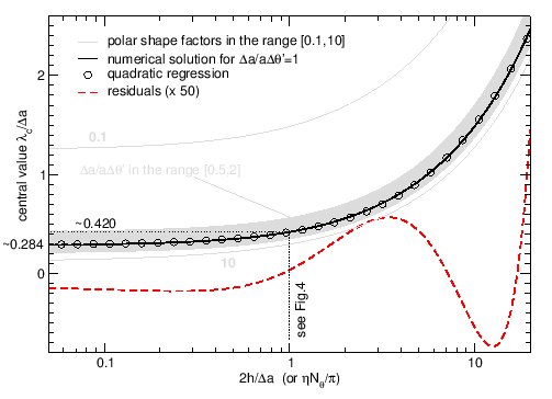
The value $\lambda_{c}\equiv\lambda(\mn@boldsymbol{r}=\mn@boldsymbol{r}_{0})$ computed at the cell’s centre is plotted versus the meridional shape factor $\frac{2h}{\Delta a}$ in Fig. 5, while holding $\frac{a_{0}\Delta\theta^{\prime}}{\Delta a}=1$ (which is a common set up in disc simulations). A parabolic fit, valid for $\frac{2h}{\Delta a}\in[0,30]$, gives

with an error of the order of a few percents. The dependency on $\frac{a_{0}\Delta\theta^{\prime}}{\Delta a}$, also indicated in the figure, is weak within reasonnable limits (see the Appendix B for a double fit of $\lambda_{c}$). Note that in the case where $h\propto\Delta a$, then $\lambda_{c}\propto h$ provided $\frac{2h}{\Delta a}\ll 1$. This special case concerns cylindrical grids with logarithmic spacing in radius and cells having a height linearly increasing with radius. However, we see that $\lambda_{c}$ is generally not proportional to the cell’s height $2h$, and this is particularly true when $\frac{a_{0}\Delta\theta^{\prime}}{\Delta a}\neq 1$. This result also goes against the standard prescription stating that $\lambda\propto h$.

In the midplane of the cell, i.e. at $Z=z_{0}$, we can rewrite Eq.(6) as follows

where $I_{\rm arc}$ must be regarded as function of $a$ and $z$ (it also depends on $\theta_{0}$ and $\Delta\theta^{\prime}$ and $\mn@boldsymbol{r}$ as well). Because $I_{\rm arc}$ is essentially regular⁴⁴ 4 In practical, $I_{\rm arc}$ has large amplitude in the very close vicinity of the arc, and not always monotonic. Even, it is logarithmically diverging as soon as the modulus $k=1$, which occurs for $R=a_{0}$ for $Z=z_{0}$. To avoid singular values, we can safely replace $k$ by $k_{*}$ in Eq.(12), where $$k_{*}^{2}[(a_{0}+R)^{2}+\zeta_{0}^{2}+\epsilon^{2}]=4a_{0}R,$$ (20) and $\epsilon=\frac{1}{100}\min\{\ell_{1},\ell_{2},\ell_{3}\}$ for instance. , we can employ a classical quadrature scheme to estimate $I_{\rm cell}$, i.e. the double integral is replaced by a discrete summation with values of $I_{\rm arc}$ taken at different places $(a,z)$. For the present purpose, Simpson’s rule has a sufficient accuracy. There are therefore $9$ nodes $(a_{i},z_{j})$ involved in total, namely

• •

  $a_{i}=a_{0}+(i-2)\frac{\Delta a}{2}$ with $i=1,2,3$,

• •

  $z_{j}=z_{0}+(j-1)\frac{h}{2}$, with $j=1,2,3$.

We then have

where the corresponding weights $w_{ij}\in\{1,4,16\}$ are given by the stencil in Fig. 6. The softening length is then deduced from Eqs.(8) and (21) where $V=a_{0}\Delta\theta^{\prime}h\Delta a$. According to Simpson’s rule, the error when estimating $I_{\rm cell}$ from Eq.(21) is of the order of $(h\Delta a)^{5}$. This makes this approach reliable enough and relatively general, at least for numerical applications based on fine cylindrical grids.

We have computed $\lambda$ from Eq.(21) and compared it with the reference¹ for the same cell’s parameter as considered in the previous example. The decimal log. of the relative error is displayed in Fig. 7. We see that accuracy is better than $10^{-4}$, except along the line where $\lambda=0$ and especially in the vicinity of the cell itself where this is rather $10\%$.

On the basis of the results above and various tests performed, we can propose a new prescription for $\lambda$ which makes the softened point mass potential very close to the Newtonian potential of a cylindrical cell by combining: i) the numerical value computed at the cell’s centre (the fit has sufficient accuracy), and ii) the $9$-point stencil. For a given cell with shape parameters $(\ell_{1},\ell_{2},\ell_{3})$ and centre $\mn@boldsymbol{r}_{0}$, the recipe is as follows:

• •

  $\lambda$ is given by Eq.(18) or Eq.(37), if $\mn@boldsymbol{r}=\mn@boldsymbol{r}_{0}$,

• •

  otherwise, $\lambda$ is given⁴ by Eqs.(8) and (21).

This composite formula is a priori easy to include into numerical codes.

By adding the contribution of individual cells, one can determine the total potential of any kind of inhomogeneous system, where each cell has its own shape parameters, density and associated softening length. We have therefore performed several concrete tests, in order to check the efficiency of this new prescription for $\lambda$. It is in particular interesting to compare with the standard prescription where $\lambda\propto h$.

Among possibilities, we have selected two configurations: i) a fully homogeneous and flat disc, and ii) a power-law density disc with constant aspect ratio. In both cases, the disc is axially symmetrical, and has inner edge at $a_{\rm in}=0.5$. The numerical grid consists of $N_{R}$ nodes in radius, and $N_{\theta}$ node in azimuth. In the vertical direction, there is a unique node located in the disc midplane. There are therefore $(N_{R}-1)(N_{\theta}-1)$ cells in total and the same amount of nodes. In practical, we use $N_{\theta}=2\times N_{R}=64$ (which leads to $\Delta\theta^{\prime}\approx 0.1$; see below for higher resolutions). In addition, we have considered two types of grid: one grid with regular spacing, and one with log. spacing. In this latter case, we have the relationship

where $\eta=h/a$ is the disc aspect ratio.

At each radius $R$ in the midplane, the reference potential is reconstructed by adding individual contributions¹. In parallel, we perform the same summation but using the Plummer potential i) with the new prescription, and ii) with the standard prescription where $\lambda\propto h$ (in practical, we take $\lambda=0.6h$). Figure 8 shows the deviations observed for the homogeneous flat disc. We see that this an improvement by $2-4$ digits depending on the radius in the disc. Results are much better close to the outer edge. We have also considered an inhomogeneous verision by simply multiplying the density field of each cell by a random factor in the range $[1,2]$. The results are plotted in the same figure and the conclusions are unchanged.

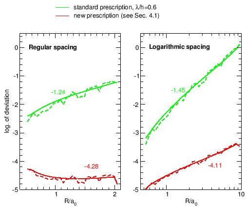
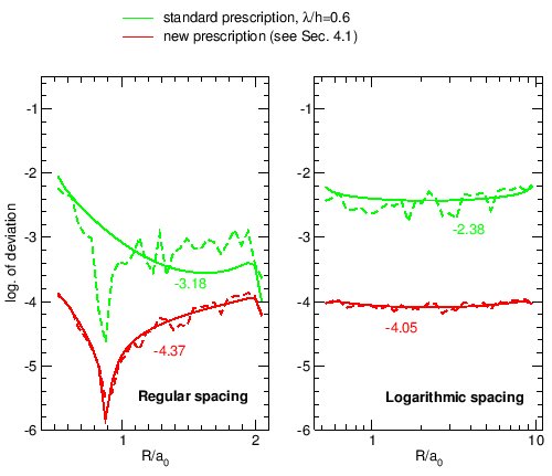
Figure 9 shows the same results but for the flared, power-law density disc where $\frac{h(a)}{a}=\frac{1}{2}\Delta\theta^{\prime}$ and $\rho(a)\propto a^{-2.5}$, which is typical. The new prescription is again better, while the benefit is a little bit reduced for the grid with regular spacing. For the grid with log. spacing, potential values are improved by almost $2$ more digits.

Figure 10 gives the deviation observed at half-sampling in radius for $N_{\theta}\in\{32,64,128,256,512,1024\}$ while maintaining $N_{R}=N_{\theta}/2$ and $a_{\rm in}=0.5$, for the two configurations considered above. This confirms that accuracy can be significantly improved by $2-3$ orders of magnitude with respect to the standard case where $\lambda\propto h$ whatever the resolution.

References

- Ansorg et al. (2003) Ansorg M., Kleinwächter A., Meinel R., 2003, MNRAS, 339, 515
- Baruteau et al. (2011) Baruteau C., Meru F., Paardekooper S.-J., 2011, MNRAS, 416, 1971
- Binney & Tremaine (1987) Binney J., Tremaine S., 1987, Galactic dynamics. Princeton, NJ, Princeton University Press, 1987, 747 p.
- Dejonghe (1987) Dejonghe H., 1987, MNRAS, 224, 13
- Durand (1953) Durand E., 1953, Electrostatique. Vol. I. Les distributions.. Ed. Masson
- Gradshteyn & Ryzhik (2007) Gradshteyn I. S., Ryzhik I. M., 2007, Table of Integrals, Series, and Products, Seventh Edition. Academic Press
- Huré (2012) Huré J.-M., 2012, Celestial Mechanics and Dynamical Astronomy, 114, 365
- Huré & Pierens (2005) Huré J.-M., Pierens A., 2005, Ap. J., 624, 289
- Huré et al. (2014) Huré J.-M., Trova A., Hersant F., 2014, Celestial Mechanics and Dynamical Astronomy, 118, 299
- Kellogg (1929) Kellogg O. D., 1929, Foundations of Potential Theory. New-York: Frederick Ungar Publishing Company
- Li et al. (2009) Li S., Buoni M. J., Li H., 2009, Ap. J. Supp. Ser., 181, 244
- MacMillan (1930) MacMillan W., 1930, The theory of the potential. No. vol. 2 in Theoretical mechanics, McGraw-Hill Book Company, inc.
- Masset (2002) Masset F. S., 2002, Aston. & Astrophys., 387, 605
- Meru & Bate (2012) Meru F., Bate M. R., 2012, MNRAS, 427, 2022
- Müller et al. (2012) Müller T. W. A., Kley W., Meru F., 2012, Aston. & Astrophys., 541, A123
- Paardekooper (2012) Paardekooper S.-J., 2012, MNRAS, 421, 3286
- Papaloizou & Lin (1989) Papaloizou J. C. B., Lin D. N. C., 1989, Ap. J., 344, 645
- Van de Vel (1969) Van de Vel H., 1969, Math. Comp., 23, 61–69
- Waldvogel (1976) Waldvogel J., 1976, Zeitschrift für Angewandte Mathematik und Physik (ZAMP), 27, 867
- Zhu (2005) Zhu P., 2005, Journal of Electrostatics, 63, 1035
Appendix A Softening length associated with the massive arc. Long-range behavior
The relative distance is given by