Discrete Sampling: A graph theoretic approach to Orthogonal Interpolation
Abstract
We study the problem of finding unitary submatrices of the discrete Fourier transform matrix, in the context of interpolating a discrete bandlimited signal using an orthogonal basis. This problem is related to a diverse set of questions on idempotents on and tiling . In this work, we establish a graph-theoretic approach and connections to the problem of finding maximum cliques. We identify the key properties of these graphs that make the interpolation problem tractable when is a prime power, and we identify the challenges in generalizing to arbitrary . Finally, we investigate some connections between graph properties and the spectral-tile direction of the Fuglede conjecture.
Index Terms:
Discrete Fourier transforms, Interpolation, Perfect graphs, Circulant graphsI Introduction
The simplest form of the question that we consider is this:
- •
Which submatrices of the discrete Fourier transform are unitary up to scaling?
For example, if from the Fourier matrix we select rows and columns then the resulting submatrix is unitary up to a factor of . This is encoded in the graph of Fig 1 and the corresponding clique shown in bold.
Answers to the bulleted question involve the structure of convolution idempotents on (integers modulo ), tiling the integers [1], maximum cliques, and perfect graphs. As different as these areas might seem, what is most striking to us is that they intersect in the fundamental problem of sampling and interpolation for discrete signals. This is the problem that first motivated us, and the work here is a sequel to [2]. While we will refer to some of the results there we have tried to make the present paper self-contained.
I-A Sampling, Interpolation, and Interpolating Bases
We need a few definitions to understand the connection to sampling and interpolation. Let be a positive integer and let . For a discrete signal the Fourier transform and its inverse are
With this definition as matrices. Multiples of the identity also occur for the submatrices we look for so, to keep from qualifying every such statement, from now on when we say “unitary” we mean “unitary up to scaling;” the multiple itself is not important. Also, the particular way our problems arise makes it more natural to seek unitary submatrices of rather than of , but the principles are the same.
We regard all discrete signals as mappings . Likewise we always consider index sets to be subsets of so that algebraic operations on their elements are taken modulo . For let
In words, is the -dimensional subspace of signals whose frequencies are zero off ; there may be additional zeros but there are at least these. We do not assume that is a band of contiguous indices (mod ), but for short we still employ the term bandlimited for a signal in .
If for some we ask if all values of can be interpolated from the sampled values with drawn from an index set . If so, we say that solves the sampling problem for and we call a sampling set. Associated with a sampling set is an interpolating basis of for which
for any . The point of an interpolating basis, as opposed to any other basis of , is that the coefficients are the components of with respect to the natural basis of . A basis of is an interpolating basis if and only if it satisfies
| (1) |
See [2] for further general properties of interpolating bases. Every has an interpolating basis but not every has an orthogonal interpolating basis, and this is the starting point of our study.
It is easy to give a criterion for the sampling problem to have a solution, and this relates sampling to submatrices of the Fourier matrix. First, in general, for an index set let be the matrix whose columns are the natural basis vectors of indexed, in order, by . Then and are respectively the column vectors of the samples of on and the samples of on . The matrix is the submatrix of with rows indexed by and columns indexed by . Then as shown in [2]:
Theorem 1
solves the sampling problem for if and only if the submatrix of is invertible.
In particular . One has
| (2) |
and the interpolation formula
expressing all the values of in terms of the sampled values on . The columns of are an interpolating basis of .
In [2] we were concerned primarily with universal sampling sets. These are the index sets for which is invertible for every index set of the same size as . So is universal if having chosen rows in according to , any choice of columns results in an invertible submatrix. In terms of the sampling problem, is a sampling set for any space , so for a universal sampling set the interpolating basis for changes with , but where to sample does not.
Theorem 1 only goes so far. We need to be able to solve (2) feasibly even in the presence of noise or numerical errors, and universality does not guarantee such stable recovery. For this we need the matrix to be well conditioned, along the lines of stability conditions imposed by other models, [3], [4]. For stable recovery the sampling set needs to be such that the energy in the samples is a a non-negligible fraction of the energy in the entire signal,
for a positive constant . This constraint is typically imposed for discrete (not necessarily timelimited) signals, [4]. In the case we are investigating (timelimited discrete signals) we would typically want to be as large as possible, uniformly over . In other words,
is equivalent to a condition on the norm of the Fourier submatrix,
which requires that all the singular values of be at least .
From this point of view, the opening question of this paper thus identifies the extreme case when has the largest possible norm, and we want to know:
- •
Given the frequency set , is it possible to find such that is unitary?
If so we say that are a unitary pair; rows of chosen according to and columns according to , like the example given in the opening paragraph. Of course, since we have that is unitary if and only if is, so being a unitary pair is symmetric in and .
It is equivalent to the preceding question to ask:
- •
Does have an orthogonal interpolating basis?
If the answer is yes then the set that indexes the orthogonal basis (and so determines where to sample) will be called an orthogonal sampling set. Our emphasis is on finding orthogonal sampling sets.
The only having an orthonormal interpolating basis is all of , while proper subspaces having an orthogonal interpolating basis cannot be too big:
Proposition 1
If has an orthogonal interpolating basis then .
We can express the symmetry of and as a unitary pair, or as orthogonal sampling sets, as:
Proposition 2
An index set is an orthogonal sampling set for if and only if is an orthogonal sampling set for .
See [2] for these results. The condition in Proposition 1 is not sufficient, but necessary and sufficient conditions for to have an orthogonal interpolating basis in the case that is a prime power, are known in the (mathematics) literature, though not in this context nor in this terminology. We will see one such result as Theorem 2 in Section II. The restriction that be a prime power also came up, in different ways, in [2]. Going beyond prime powers is an unmistakeable challenge.
Our approach to the problem opens with an important connection between orthogonal sampling sets and the algebraic structure of the zeros of an idempotent on that comes from a given , where is the indicator function of . We then introduce the difference graph of an idempotent, recasting the problem of finding orthogonal sampling sets in graph theoretic terms as a search for maximum cliques, the key contribution of this paper. This is of more than theoretical interest because we show, in section III-A that when is a prime power the difference graphs we consider are perfect graphs, and hence the problem of finding a maximum clique is tractable. We provide some insights into the challenges in generalizing such a result when is not a prime power, in section V. We also investigate the clique, chromatic and Lovász numbers of these graphs in Section VI and their relationship to the Fuglede conjecture. We conclude with some interesting open problems.
We are happy to thank many colleagues for their interest, in particular Maria Chudnovsky, Sinan Gunturk, and Mark Tygert. We also thank Sivatheja Molakala, a close friend of the first author, and we dedicate this paper to his memory.
I-B Related work on compressed sensing
A somewhat related problem comes up in construction of Fourier sub-matrices with the restricted isometry property. The problem in this context is to find a set of rows such that
for any length vector that has at most entries [5]. Thus, here the objective is to find a set of rows such that regardless of the choice of columns, the resulting matrix is approximately unitary. Most of the initial constructions of such were random [6], [7]. Deterministic construction of such has been harder, but significant developments were made in [8], [9] and [10], for example. In contrast, for the problem currently under investigation; we are given a set of columns , and we wish to find a set of rows such that the resulting square submatrix is unitary.
II Idempotents on and their Zero-sets
There is a natural, one-to-one correspondence between index sets and idempotents for convolution, and properties of one can be used to study properties of the other. Given let be its indicator function. Since the function
| (3) |
is an idempotent, and by definition of . We write simply if the set is clear from the context. Conversely, if an idempotent is given then its Fourier transform, having values in , is the indicator function for an index set.
The following lemma opens the way to a very diverse set of phenomena. A similar result, in a much different context, holds for discrete signals in ; see [1].
Lemma 1
An index set is an orthogonal sampling set for if and only if and for , .
Proof:
Recall that a matrix is circulant if and only if it is diagonalized by the Fourier transform. Consider the matrix
Since is a diagonal matrix with the diagonal equal to , it follows that the matrix is circulant, with first column . Hence the matrix is a submatrix of the circulant matrix , with rows and columns both indexed by ; in other words, the entires of the matrix are given by where . Now if is unitary, then is diagonal, which implies
∎
In geometric terms, defines the orthogonal projection via
The orthogonal complement to is where is the complement of .
The proof of Lemma 1 is in keeping with the question we asked at the beginning of the paper, but it is worth pointing out an essentially equivalent approach. Let be the shift , and write
It is straightforward to check that the inner product of two shifted ’s is
Any shift of is also in and thus an index set having the property that for , determines a set of orthogonal vectors in . When is an orthogonal sampling set we normalize as in (1) to then obtain an orthogonal interpolating basis for given by
| (4) |
This is the recipe for turning an orthogonal sampling set into an orthogonal interpolating basis. All vectors in an orthogonal interpolating basis have length .
In view of Lemma 1 we introduce the zero-set of the idempotent associated with a given ,
Note that
so in particular is never in . We also observe the symmetry relation
| (5) |
implying that both and either are or are not in .
It is important for our work that the zero-set has a very particular algebraic structure. Let
| (6) |
be the set of divisors of that are . Then:
Lemma 2
If is an idempotent then its zero-set is the disjoint union
for a set of divisors , where
| (7) |
Here is the greatest common divisor of and . The equivalence relation if already partitions into the disjoint union
We also have
where is the multiplicative group of units in the ring , so is times the elements in that are coprime to . In brief, the lemma says that the zero-set of an idempotent is essentially the disjoint union of multiplicative groups.
See [11], for example, for a version of this result. The proof in the prime power case is elementary enough, and is reproduced in Section A.
We note one quick corollary.
Corollary 1
If is prime then either or . In the latter case .
Proof:
If there is a then we must have and . In this case and , so . ∎
We refer to , which we now know to be , as the zero-set divisors of . It is helpful to describe all at once as
| (8) |
and then to restate Lemma 1 as saying that is an orthogonal sampling set for if and only if
| (9) |
II-A A converse to Lemma 2?
To study orthogonal sampling sets we will need both Lemma 2 and a converse. The converse would ask to find an idempotent whose zero-set is a prescribed disjoint union of multiplicative groups, and this cannot be done in all cases. For example, let and . The set can be presented in the form given in Lemma 2, namely , but an exhaustive search shows that there is no idempotent on with .
There are some cases for which we can easily settle the existence of a converse. For example, when is a prime power, the converse to Lemma 2 is known to be true. Given a divisor set , the index set with zero set divisors can be constructed as ([12])
We note that the size of constructed above is . This is the general form any that has an orthogonal sampling set:
Theorem 2
Let . Then has an orthogonal sampling set if and only if .
III Difference Graphs and Maximal Cliques
When is a prime power Theorem 2 gives a complete answer to the question of when a space has an orthogonal sampling set. We can formulate the problem in the language of graph theory, and this has significant consequences because of the special structure of the graphs involved.
Let be the graph with vertices from , and with an edge between two vertices if . We call this the difference graph of . We will also denote the graph so constructed as or simply , wherever appropriate. At this point we want to note that though such graphs can be constructed from any set of divisors , it is not clear if the set of divisors comes from an idempotent. A converse of Lemma 2 is required to make such a claim.
First, let make some comments on the structure of difference graphs. These graphs are Cayley graphs [13] defined on a cyclic group, and hence circulant, which itself is enough to characterize some connectivity properties of the graphs (difference graphs are regular, for example). There is some work in literature on the structure of such graphs. Since, according to Lemma 2, the zero-set can be written , as in (8), our difference graphs are also what have been called GCD-graphs, see [14]. Note that GCD-graphs can be constructed starting from any divisor set , but for difference graphs these divisor sets must come from an idempotent. Thus difference graphs are a subclass of GCD-graphs: see [14], [15] for some results on the clique and chromatic numbers of GCD-graphs. In this paper we are primarily interested in the structure of maximum cliques and perfectness of these graphs, and in this section we will show that in several cases is a perfect graph. Figures 2 and 3 are two pictures of difference graphs generated with Mathematica.
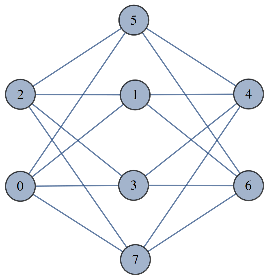

The key observation relating orthogonal sampling sets to difference graphs comes from Lemma 1, which we restate as
Lemma 3
An index set of size is an orthogonal sampling set for if and only if determines a maximum clique in .
Proof:
Any orthogonal sampling set determines a clique in . Conversely, any clique whose size is equal to the dimension of determines an orthogonal sampling set. The clique determined by an orthogonal sampling set must be a maximum clique because it determines an orthogonal basis of . That is, if a clique (sampling set) can be made larger by adding a vertex then, by definition of , the set also satisfies
This means that is an orthogonal sampling set for which is a contradiction since . ∎
The following corollary, when combined with Lemma 3, is essentially a restatement of Theorem 2 in terms of cliques. It is interesting to put it this way because the statement pertains just to idempotents with no references to sampling, orthogonal bases, etc.
Corollary 2
Let be a prime power and let be an idempotent. Then any maximum clique in the difference graph is of size .
III-A Perfect difference graphs
Since orthogonal sampling sets correspond to maximum cliques in a difference graph, it is natural to relate the sampling problem to the graph-theoretic (and computational) question of finding maximum cliques. Finding cliques takes exponential time for generic graphs, but in our case the difference graphs have enough structure to solve the problem in polynomial time – the graphs are perfect when is a prime power, and in two other cases that we know. Recall that a graph is perfect if for every induced subgraph the chromatic number is equal to the size of a maximal clique.
Theorem 3
Let be an idempotent and let be the associated difference graph. Then is perfect when: (a) ; (b) , the product of two primes; (c) and are such that and , where .
In all cases we prove that is a Berge graph. The result then follows from the celebrated Strong Perfect Graph Theorem, [16], which states that a graph is perfect if and only if it is a Berge graph. Recall that a graph is a Berge graph if every odd cycle with five or more nodes in or in (the complement of ) has a chord. Under each of the assumptions on the proofs proceed via a series of case distinctions.
Suppose that form a cycle in . Then , or , say, with . Similarly . We can thus write and for some coprime to . Now consider the following cases.
Case 1: . In this case, . Since , we have . This means that , and so we have a chord between and .
Case 2: .
As in Case 1, we have . Since we have , and so there is a chord between and .
Case 3: .
Suppose we have . Then leads us to , which need not be in . Hence there need not be an edge between and .
Now, , and so for some coprime to . If , then we have a chord between and , by the same argument in Case 1 applied to . This leaves us with the case . Now we have . Since and is coprime to , it follows that and so . Hence we have an edge between and .
In all cases the cycle has a chord.
A similar proof holds for cycles in , with replaced by which, in this case, is still a set of prime powers. Thus every odd cycle in and in with at least 5 nodes has a chord and we conclude that is a Berge graph, hence perfect.
In fact we have proved that for the difference graphs are free or cographs [17].
Part (b), : Then . Take the extreme case, when . Then by Lemma 2 the zero-set is the set of all nonzero indices, . So all the vertices in the difference graph are connected to each other and every cycle has a chord, while . The remaining cases to show that is perfect are then covered by part (c).
Now to part (c) of the theorem. In the following we will take a cycle of size five, but the argument can be generalized to any cycle of odd size. Assume that form a cycle in . Let . Since is at most of size there are two cases.
Case 1: , i.e. includes a prime.
In this case all the are divisible by either of at most two primes, say and . For the cycle not to have a chord between vertices , we need to be coprime to both and . Now consider any two consecutive edges, say and . Suppose both these edges correspond to divisibility by the same prime, i.e., both and are divisible by, say, . It follows that is divisible by as well, which means the edge exists in . Hence all consecutive edges must correspond to divisibility by different primes, as indicated in Fig. 4. However since the cycle is odd in size, this is impossible.
Case 2: . Since , we can assume that . In this case all the are coprime to . For a chord not to exist, must be divisible by either or , and thus each chord falls into one of these two groups. Now consider two adjacent chords , say and , as in Fig. 5. Then both and should be divisible by different primes, for otherwise would be divisible by as well. But this too is impossible according to the following purely geometric observation:
Lemma 4
Consider a polygon with vertices, where is odd. We call two chords (diagonals) of adjacent if they form a triangle with one of the sides of (For example as in Fig. 5). Then it is impossible to divide the chords into two groups such that adjacent chords belong to different groups.
Proof:
Once again we make some case distinctions.
Case 1: Suppose the chords in each group are represented by drawing them dashed and dotted, respectively. Assuming the chord to be dotted, we can dash/dot the remaining chords (see Fig. 6). We end up with chord which has to be both dashed and dotted, a contradiction.
Case 2: The argument is similar to the previous case. Assume is dotted. Then we can mark the remaining chords as dashed and dotted, as in Fig. 7. There is no way to mark the chord consistently. ∎
IV Further comments for
In the case when , Theorem 3 establishes that any difference graph is perfect, and maximum cliques can be determined in polynomial time. In fact, for we can say more: all difference graphs (and their complements) are well covered [18]. In other words, any maximal clique is maximum, and so maximum cliques can be found by a simple greedy algorithm.
Theorem 4
When , all maximal cliques in the difference graph are of size .
Proof:
We prove this by induction on . Suppose is the largest divisor in . For any maximal clique in , we note that is a maximal clique in and so
Any element of is of the form for , and for two elements and of with , must be coprime to . Thus it follows that for to be maximal, takes on all the values , and so
For the case when , the size of any maximal clique is , thus completing the proof. ∎The theorem is not true for arbitrary . As an example, consider and . In the difference graph , we note that is maximal, and so is .
IV-A Counting the number of orthogonal sampling sets
Lemma 3 allows us to count the number of orthogonal sampling sets. We first find the number of orthogonal sampling sets for a given with , for this let denote the number of maximal cliques in for a set of divisors of .
Lemma 5
Suppose is a prime power. Let be a non empty set of divisors of , and let be the smallest element of . Then, the number maximal cliques is given by
where
If is empty, we have
Proof:
Note that if is empty, every vertex is a max clique (max clique size is by Theorem 2) and so the number of max cliques is simply the number of vertices in the graph, i.e. .
Now assume is non empty. First we establish the result assuming . For any maximal clique of , consider the congruence classes modulo :
Note that for any ,
- •
, so , and
- •
.
Combining these two, we note that
Thus we see that any clique in is composed of cliques from . Each of these cliques is multiplied by , and ‘raised’ to a different congruence class modulo , and taking the union of these ‘raised’ cliques gives us a clique in . We note that this correspondence is one-to-one, and so
thus completing the proof.
Now consider the case for an arbitrary smallest divisor (not necessarily ). For any two elements of a maximal clique , we see that , so that
It follows that all elements of are divisible by . At this point we note that the number of possible ways to pick given is simply, : the number of congruence classes modulo .
Now note that for any ,
so that . So if we consider , we see that is a clique in . Since , the number of ways to construct , from the previous paragraph, is
Since the number of ways to construct the translate is , the theorem follows.
∎
We next focus on finding the total number of maximal cliques of size in . Suppose with . To expand upon the recursion from Lemma 5, first note that the smallest element of is . We can define
to continue the recursion. We see that
where we take . Now we also take , and let
Then represents the ‘gap’ between successive divisors in . Note that
So we have
Lemma 6
Suppose is a prime power. The number of orthogonal sampling sets for is given by where
where with , and .
We obtain the total number of orthogonal sampling sets of size by summing over all possible that sum to :
From the form of this expression we observe that the count is given by a -fold convolution:
where is
The generating function of is
so the generating function for is the product of individual generating functions. In conclusion:
Theorem 5
For prime powers and , define the generating function
| (10) |
The number of orthogonal sampling sets of size in is the coefficient of in . ∎
To get an idea of the numbers, we plot
Figures 9 and 10 plot vs for various prime powers . The function is not equal to the linear function that jumps out in the plots, but in the examples we have tried it appears to be remarkably close.


For an example of Theorem 5, when and we have
The number of orthogonal sampling sets of size in is the coefficient of , which we find to be . This is out of a total of index sets of size . The number of orthogonal sampling sets of size in is the coefficient of , which is , and is out of .
V Perfectness for arbitrary
The case of having more than one prime factor assumes significance when dealing with higher dimensional orthogonal interpolation. For example, in the typical two dimensional setting, suppose we assume each of the dimensions to be and respectively ( are primes). The resulting two dimensional orthogonal interpolation problem can be easily seen to be equivalent to a one dimensional orthogonal interpolation problem with [12]. Investigating the relationship between existence of orthogonal sampling sets and properties of the corresponding difference graph for an arbitrary dimension is an intriguing question, which we attempt to address in this section. One naturally interesting question is to what extent perfectness, as in Theorem 3, holds.
Examples disproving perfectness and other properties for GCD-graphs [14], [15] cannot directly apply to difference graphs. Here is an example. Let and let (all elements of whose greatest common divisor with is or ). We take to be the GCD-graph determined by , i.e., there is an edge between and if . Now consider the nodes . Figure 8 shows the cycle on these nodes, and is not perfect (this example is due to Sivatheja Molakala). But we do not know if is the zero-set of an idempotent. It is computationally infeasible to check this, and we do not know to what extent the converse of Lemma 2 holds when is not a prime power.
As a special case, when is a singleton the graph becomes a unitary Cayley graph, [19], and such graphs are shown to be perfect when either is even or is odd with at most two prime factors. When is a singleton, a converse to Lemma 2 can easily be seen to be true [12], and thus the result of [19] generalizes Theorem 3 to arbitrary when is a singleton. For of arbitrary size; perfectness of the difference graph has not been investigated, nor has the existence of an idempotent that generates . Thus, in addition to investigating GCD-graphs thoroughly, a more encompassing converse to Lemma 2 is crucial for investigating the higher dimensional interpolation problem.
The next natural question is to ask if we can impose specific restrictions on such that the corresponding difference graph is perfect. For reasons to be elaborated on in Section VI, one reasonable restriction we could think of is that should tile . Take for instance , it can be verified that satisfies the following properties of interest:
- 1.
The index set tiles with , in other words the sumset is equal to , and
- 2.
The bandlimited space has an orthogonal sampling set.
Finding , we see that . Consider the induced cycle shown in Figure 11, which proves that is not perfect. This suggests that perfectness is not likely the correct property to investigate for a general .
VI Clique, chromatic and Lovász numbers
In this section, we attempt to investigate the clique, chromatic numbers (their gap in particular), and their implications for the underlying bandlimited space . Denote the size of the largest clique in by , and the chromatic number by . Recall that , and the chromatic gap is zero if the difference graph is perfect.
Also recall that is the graph on the same vertices as formed with the edges that are missing from . In our case, we see that for a difference graph , corresponds to the difference graph constructed from the divisors that are missing from , i.e.
Next, the Lovász number ([20]) is
where is a unit vector and is an orthonormal representation of , i.e.
Here denotes the standard inner product. The Lovász number is sandwiched between the clique number and the chromatic number of :
For difference graphs constructed from , we know from Lemma 1 that , and in particular if has an orthogonal sampling set then . The following theorem is a stronger version of this observation.
Theorem 6
Let be a difference graph constructed from an idempotent . Then , where is the Lovász number ([20]) of the graph . If has an orthogonal sampling set, then .
Proof:
Note that are connected in a difference graph only if . Thus forms an orthonormal representation of , and so
Fix some , and let be the corresponding canonical basis vector. Set to be the unit vector . Then since , we obtain
Since , it follows that . Moreover, if has an orthogonal sampling set then we have , and thus .
∎An even stronger version of Theorem 6 would require us to investigate if the chromatic number of is bounded by . While we are unable to verify this, we do have one interesting observation.
Theorem 7
Suppose has an orthogonal sampling set, and be the associated difference graph. If the chromatic number of is equal to then and any max clique in tiles .
We say that a set tiles if there exists a set of translates such that every can be written uniquely as , with , .
Proof:
Suppose is a max-clique in and is a max-clique in . If and satisfy
then , a contradiction, as and correspond to complementary sets of divisors of . Thus all the sums in the sumset are distinct, and so is of size . In particular, if , then , and tiles .
Now for the given difference graph ,
and so the theorem follows. Note that implies that every element of can be written uniquely as
where and . We can see that the mapping is a coloring of : If are adjacent in then would imply , a contradiction. Thus we have a coloring with colors: in other words when has an orthogonal sampling set then is equivalent to . ∎
If is perfect, for example when is a prime power, or when the hypothesis of Theorem 3 holds, then the chromatic number and clique number for are equal, and Theorem 7 applies. Thus for prime power , if a bandlimited space has an orthogonal sampling set , then tiles . This is a well known result, see for eg [11], and a special case of the Fuglede’s Conjecture, also known as the spectral set conjecture. This conjecture first appeared in [21] and asks, in other language, whether the above result holds in greater generality.
VI-A Fuglede’s conjecture
A spectral set is a domain for which there exists a spectrum such that is an orthogonal basis for . Then
Conjecture (Fuglede , [21], Spectral-Tile direction): If a domain is a spectral then it tiles .
The original result of Fuglede contained a proof of this conjecture under the assumption that is a lattice subset of . Since then the conjecture has been proved to be true under more restrictive assumptions on the domain ; for e.g. for convex planar sets [22] and union of intervals [23]. Further, the conjecture has been disproved in [24]. For cyclic groups , the conjecture is known to be true the case when is a prime power, see for e.g. [25], [26] and [11]. The conjecture for , primes was proved in [27]. Other domains where Fuglede’s conjecture is known to be true includes the field of adic numbers [28, 29] and [30]. See [31] for the relationship between validity of conjectures in various domains.
Thus strengthening Theorem 6 further,by proving a similar statement in terms of the chromatic number of , would prove Fuglede’s conjecture (in the Spectral-Tile direction) for .
VII Conclusion and open problems
Given a bandlimited space, we defined a difference graph such that the problem of existence and computation of orthogonal interpolating bases becomes equivalent to the problem of finding cliques in the difference graph. When is a prime power, difference graphs have nice structural properties, including perfectness, that have consequences for finding cliques and hence for orthogonal interpolation.
However, for the case when is a prime power, since orthogonal interpolation has been otherwise well investigated, the more relevant (and interesting) situation is when is not a prime power. In this case, we provided examples of difference graphs (coming from idempotents) that are not perfect. It is not clear what perfectness implies for the corresponding idempotent, and vice versa.
We also observed that properties of the difference graph are closely related to tiling and spectral properties. For instance, we have not yet found a counter example to the following observation on difference graphs:
Conjecture 1
Suppose has an orthogonal sampling set, and be the associated difference graph. Then or equivalently .
If Conjecture 1 is true, Fuglede’s conjecture for ([21]) follows in the Spectral-Tile direction via Theorem 7.
We have also been unable to prove or provide a counter example to the following weaker version of conjecture 1. If then divides , and so we propose:
Conjecture 2
If is a difference graph constructed from an idempotent , then the size of any max clique in divides .
When is a prime power, conjecture 2 follows trivially from Theorem 4. For general , this conjecture can be proved when is a singleton ([19]). For arbitrary GCD-graphs, conjecture 2 fails: consider - this example is from [14]. This GCD-graph has a maximal clique size of , thus it seems to provide a counter-example to conjecture 2. However, an exhaustive search shows that does not come from an idempotent, so Conjecture 2 still remains to be resolved.
Appendix A Proof of Lemma 2
Proof:
We show that if and then , in other words, if vanishes at one element of an then it vanishes on all of . This will prove the result.
Introduce the polynomial
| (11) |
To say that is to say that . The order of is and is a root of the cyclotomic polynomial
Since divides any monic polynomial that vanishes at a primitive ’th root of unity it divides , and it follows that must vanish at all the with .
Now consider evaluating for coprime to . We have
But is also a primitive ’th root of unity, hence a root of and in turn a root of . ∎
References
- [1] B. Farkas, M. Matolcsi, and P. Móra, “On Fuglede’s conjecture and the existence of universal spectra,” Journal of Fourier Analysis and Applications, vol. 12, no. 5, pp. 483–494, 2006.
- [2] B. Osgood, A. Siripuram, and W. Wu, “Discrete sampling and interpolation: Universal sampling sets for discrete bandlimited spaces,” IEEE Trans. Information Theory, vol. 58, no. 7, pp. 4176–4200, 2012.
- [3] H. Landau, “Necessary density conditions for sampling and interpolation of certain entire functions,” Acta. Math., vol. 117, pp. 37–52, 1967.
- [4] R. Bass and K. Gröchenig, “Random sampling of multivariate trigonometric polynomials,” SIAM J. Math. Anal, vol. 36, p. 795, 2004.
- [5] E. J. Candes, J. K. Romberg, and T. Tao, “Stable signal recovery from incomplete and inaccurate measurements,” Communications on pure and applied mathematics, vol. 59, no. 8, pp. 1207–1223, 2006.
- [6] E. J. Candes and T. Tao, “Near-optimal signal recovery from random projections: Universal encoding strategies?” IEEE transactions on information theory, vol. 52, no. 12, pp. 5406–5425, 2006.
- [7] M. Rudelson and R. Vershynin, “On sparse reconstruction from fourier and gaussian measurements,” Communications on Pure and Applied Mathematics, vol. 61, no. 8, pp. 1025–1045, 2008.
- [8] P. Xia, S. Zhou, and G. B. Giannakis, “Achieving the welch bound with difference sets,” IEEE Transactions on Information Theory, vol. 51, no. 5, pp. 1900–1907, 2005.
- [9] J. Haupt, L. Applebaum, and R. Nowak, “On the restricted isometry of deterministically subsampled fourier matrices,” in Information Sciences and Systems (CISS), 2010 44th Annual Conference on. IEEE, 2010, pp. 1–6.
- [10] G. Xu and Z. Xu, “Compressed sensing matrices from fourier matrices,” IEEE Transactions on Information Theory, vol. 61, no. 1, pp. 469–478, 2015.
- [11] E. M. Coven and A. Meyerowitz, “Tiling the integers with translates of one finite set,” Journal of Algebra, vol. 212, no. 1, pp. 161–174, 1999.
- [12] A. Siripuram, “Sampling and interpolation of discrete signals: Orthogonality, universality and uncertainty,” Ph.D. dissertation, Stanford University, 2014.
- [13] C. Godsil and G. F. Royle, Algebraic graph theory. Springer Science & Business Media, 2013, vol. 207.
- [14] M. Bašić and A. Ilić, “On the clique number of integral circulant graphs,” Applied Mathematics Letters, vol. 22, no. 9, pp. 1406–1411, 2009.
- [15] A. Ilić and M. Bašić, “On the chromatic number of integral circulant graphs,” Computers & Mathematics with Applications, vol. 60, no. 1, pp. 144–150, 2010.
- [16] M. Chudnovsky, N. Robertson, P. Seymour, and R. Thomas, “The strong perfect graph theorem,” Ann. Math., vol. 164, no. 1, pp. 51–229, 2006.
- [17] A. Brandstädt, V. B. Le, and J. P. Spinrad, Graph classes: a survey. SIAM, 1999.
- [18] M. D. Plummer, “Well-covered graphs: a survey,” Quaestiones Mathematicae, vol. 16, no. 3, pp. 253–287, 1993.
- [19] W. Klotz and T. Sander, “Some properties of unitary Cayley graphs,” Electronic Journal of Combinatorics, vol. 14, no. 1, p. R45, 2007.
- [20] L. Lovász, “On the shannon capacity of a graph,” IEEE Transactions on Information theory, vol. 25, no. 1, pp. 1–7, 1979.
- [21] B. Fuglede, “Commuting self-adjoint partial differential operators and a group theoretic problem,” Journal of Functional Analysis, vol. 16, no. 1, pp. 101–121, 1974.
- [22] A. Iosevich, N. Katz, and T. Tao, “The Fuglede spectral conjecture holds for convex planar domains,” Mathematical Research Letters, vol. 10, no. 5, pp. 559–569, 2003.
- [23] I. Łaba, “Fuglede’s conjecture for a union of two intervals,” Proceedings of the American Mathematical Society, vol. 129, no. 10, pp. 2965–2972, 2001.
- [24] T. Tao, “Fuglede’s conjecture is false in 5 and higher dimensions,” arXiv preprint math/0306134, 2003.
- [25] I. Laba, “The spectral set conjecture and multiplicative properties of roots of polynomials,” Journal of the London Mathematical Society, vol. 65, no. 03, pp. 661–671, 2002.
- [26] T. Tao, “Some notes on the Coven-Meyerowitz conjecture,” https://terrytao.wordpress.com/2011/11/19/some-notes-on-the-coven-meyerowitz-conjecture/#more-5470, 2011.
- [27] R.-D. Malikiosis and M. N. Kolountzakis, “Fuglede’s conjecture on cyclic groups of order ,” arXiv preprint arXiv:1612.01328, 2016.
- [28] A. Fan, S. Fan, and R. Shi, “Compact open spectral sets in ,” Journal of functional analysis, vol. 271, no. 12, pp. 3628–3661, 2016.
- [29] A. Fan, S. Fan, L. Liao, and R. Shi, “Fuglede’s conjecture holds in ,” arXiv preprint arXiv:1512.08904, 2015.
- [30] A. Iosevich, A. Mayeli, and J. Pakianathan, “The fuglede conjecture holds in ,” Analysis & PDE, vol. 10, no. 4, pp. 757–764, 2017.
- [31] D. E. Dutkay and C.-K. LAI, “Some reductions of the spectral set conjecture to integers,” in Mathematical Proceedings of the Cambridge Philosophical Society, vol. 156, no. 01. Cambridge Univ Press, 2014, pp. 123–135.