Uncovering Droop Control Laws Embedded Within the Nonlinear Dynamics of Van der Pol Oscillators

The nominal system frequency is denoted by $\omega$, and for the $j$th inverter, the instantaneous phase angle, $\phi_{j}$, evolves as

where $\theta_{j}$ represents the phase offset with respect to the rotating reference frame established by $\omega$. Denote the instantaneous current injected by the $j$th inverter by $i_{j}(t)$ and its instantaneous terminal voltage by $v_{j}(t)$. Since we are primarily interested in harmonic signals, we parameterize the instantaneous voltage as $v_{j}(t):=r_{j}(t)\cos(\omega t+\theta_{j}(t))$, where $r_{j}(t)$ is the instantaneous terminal-voltage amplitude. We define the instantaneous active- and reactive-power injections [33, 34]

Assuming the fundamental frequency of the current injected by the $j$th inverter is $\omega$, the average active and reactive power over an AC cycle (of period $2\pi/\omega$) are then given by

In general, the time average of a periodic signal $u_{j}$ with period $T$ is denoted by $\overline{u}_{j}$, and defined as:

Subsequent developments will leverage signals represented in the scaled time coordinates $\tau=\omega t$, and for the continuous-time signal $x$, we will denote $\dot{x}=\frac{d}{d\tau}x$.

For the $N$-tuple, $\{x_{1},\dots,x_{N}\}$, denote $x=[x_{1},\dots,x_{N}]^{\mathrm{T}}$ to be the corresponding column vector; $(\cdot)^{\mathrm{T}}$ denotes transposition. The cardinality of the set $\mathcal{X}$ is denoted by $|\mathcal{X}|$; $[X]_{ij}$ isolates the entry in the $i$th row and $j$th column of matrix $X$. $\mathbb{R}^{N}$ is the space of $N\times 1$ real-valued vectors, $\mathbb{T}^{N}$ is the $N$-torus. Given a scalar function $f(x)$, $\nabla_{x}f(x)$ returns the gradient $[\frac{\partial f}{\partial x_{1}},\ldots,\frac{\partial f}{\partial x_{n}}]^{\mathrm{T}}$. Finally, $\mathrm{diag}\{x_{1},\dots,x_{N}\}$ denotes a diagonal matrix with diagonal entries given by $x_{1},\dots,x_{N}$.

For resistive networks, droop control linearly trades off frequency deviation versus reactive-power; and inverter terminal-voltage amplitude versus active-power [2, 35]:

where ${\overline{Q}_{j}^{*}}$ and $\overline{P}_{j}^{*}$ are the per-phase average reactive-power and active-power setpoints, respectively; $\overline{r}_{j}^{*}$ is the terminal-voltage-amplitude setpoint; and $n_{j},m_{j}\in\mathbb{R}_{>0}$ are reactive-power and active-power droop coefficients, respectively. As expressed in (5), we assume that the droop laws are executed with AC-cycle averages of active and reactive power. To preserve the generality of the ensuing discussions, we disregard the dynamics of additional low-pass filters, voltage controllers, and current controllers in experimental implementations [3]; however, these could be included in the analysis readily.

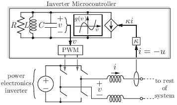
Consider the Van der Pol oscillator to constitute the virtual oscillator circuit for inverter control as shown in Fig. 2. The circuit implementation is composed of a parallel $RLC$ circuit and a nonlinear voltage-dependent current source, $g(\cdot)$. In the scaled time coordinates $\tau=t/\sqrt{LC}$, the dynamics of the oscillator are captured by the following:¹¹ 1 For notational simplicity, we drop the subscript from electrical quantities and parameters that indexes the inverter in this section.

where $u(\tau)$ is the current input to the Van der Pol oscillator (see Fig. 2), and $\kappa$ is the current gain. In particular, the inverter output current is scaled by $\kappa$, and this is extracted from the Van der Pol oscillator that forms the inverter controller. The system in (6) can be compactly written as

by defining the following parameters:

With this notation in place, the nonlinear voltage-dependent current source is a cubic polynomial, $g(v)=v-\beta(v^{3}/3)$ (see Fig. 2). Liénard’s condition [12] for ensuring a stable limit cycle in the system (7) requires positive damping at the origin, i.e., $\alpha=\sigma-{1}/{R}>0$. In the so-called quasi-harmonic limit, i.e., $\varepsilon\searrow 0$, the model (7) reduces to a forced harmonic oscillator with unit frequency. In the original time scale $t=\tau\sqrt{LC}$, this natural frequency of oscillation is $1/\sqrt{LC}$. By standard regular perturbation arguments [13, Theorem 10.1], this correspondence can also be made for $\varepsilon$ sufficiently small. In subsequent developments, with reference to (1), and to compare the droop-control system (5) and the VOC system (6), we set $\omega=1/\sqrt{LC}$.

We begin by establishing a state-space model in Cartesian coordinates; choosing a scaled version of the inductor current and capacitor voltage as states, $x:=\varepsilon i_{L}$, and $y:=v$, we get

Next, we transform the model (9) to polar coordinates by defining $x=r\sin(\phi)$ and $y=r\cos(\phi)$. We recover the following dynamics in polar coordinates:²² 2 This bijective change of coordinates is well defined (and leads to smooth dynamics) whenever $r\neq 0$ or equivalently $[x,y]^{\mathrm{T}}\neq 0$. In Theorem 2, we establish well-posedness conditions focused on convergence of the amplitude dynamics to an equilibrium that excludes the origin.

In ensuing discussions, we will leverage (10) written in the original time coordinates, with the nominal frequency of oscillation, $\omega=1/\sqrt{LC}$, and phase offset as defined in (1):

Consider two microgrids, each with $N$ identical inverters, identical network configurations and loads. All inverters in one microgrid are controlled with VOC (11), and the inverters in the other are controlled with droop control (5). For the $j$th inverter, denote the difference in voltage amplitudes and phase offsets in the two inverter-control strategies by

where $\bar{r}_{j}$ and $\bar{\theta}_{j}(t)$ are the amplitudes and phases as used in droop control (5), and $r_{j}(t)$ and $\theta_{j}(t)$ those in VOC (11).

In the following, we analyze how the droop laws and coefficients should be designed so that the difference in the phase dynamics and steady-state equilibrium voltage profile of the two sets of inverters (controlled with VOC and droop) is of order $\mathcal{O}(\varepsilon)=\mathcal{O}(\sqrt{L/C})$. To bridge the time-scale separation between VOC (that is implemented in real-time) and droop control (that presumes the existence of a quasi-stationary sinusoidal steady state), we average the VOC dynamics (11) (a detailed derivation is provided in Step 1 of the proof to Theorem 1 below) to arrive at the following description:

The averaged VOC dynamics (14) enable us to compare the droop control laws in (5) with VOC (11).

The correspondences derived in Theorem 1 are asymptotic results based on a perturbation and averaging analysis for sufficiently small $\varepsilon=\sqrt{L/C}$. However, a small $\varepsilon$ also implies a weak (nonlinear) viscous damping in (7) and a slow convergence to the quasi-harmonic limit cycle. In Section V-C, we show that the convergence rate is, in fact, inversely proportional to $\varepsilon$. Theorem 1 and the above discussion indicate that the droop laws (5) are recovered from the VOC dynamics (11) only on slow AC-cycle time scales, and when the dynamics of VO-controlled inverters are deliberately decelerated. Hence, on the limit cycle, the decelerated VOC subsumes droop control, but it is much faster in general. Finally, the correspondences established in (16) and (17) are formally valid only on a bounded time horizon $[0,t^{*}]$. The findings can be extended to an unbounded time horizon provided that the averaged system is exponentially stable [13]. In Section IV, we establish such exponential stability results.

We assume balanced three-phase operation and all electrical quantities referred henceforth are with respect to a per-phase equivalent network. The nodes of this per-phase equivalent electrical network are collected in the set $\mathcal{A}$, and branches (edges) are collected in the set $\mathcal{E}:=\{(j,\ell)\}\subset\mathcal{A}\times\mathcal{A}$. Let $\mathcal{N}:=\{1,\dots,N\}\subseteq\mathcal{A}$ denote nodes that the inverters are connected to, and denote the set of internal nodes as $\mathcal{I}:=\mathcal{A}\setminus\mathcal{N}$. Shunt loads—modeled as parallel combinations of resistances and/or constant (in a synchronous $\mathrm{dq}$-frame) current sources—are connected to $\mathcal{I}$.

Denote the vectors that collect the nodal current injections and node voltages in the network by $i_{\mathcal{A}}$ and $v_{\mathcal{A}}$, respectively. To be precise, $i_{\mathcal{A}}$ and $v_{\mathcal{A}}$ are real-valued functions of time. The coupling between the inverters is described by Kirchhoff’s and Ohm’s laws, which read in matrix-vector form as

where, entries of the conductance matrix $Q_{\mathcal{A}}\in\mathbb{R}^{|\mathcal{A}|\times|\mathcal{A}|}$ are

with $g_{j}\in\mathbb{R}_{\geq 0}$ denoting the shunt (load) conductance at node $j$, and $g_{j\ell}=g_{\ell j}\in\mathbb{R}_{\geq 0}$ the conductance of the line $(j,\ell)$.

Let $i\!=\![i_{1},\dots,i_{N}]^{\mathrm{T}}$ and $v\!=\![v_{1},\dots,v_{N}]^{\mathrm{T}}$ be the vectors of inverter current injections and terminal voltages, respectively, and let $i_{\mathcal{I}}$ and $v_{\mathcal{I}}$ be the vectors collecting the current injections and nodal voltages for the interior nodes.⁴⁴ 4 We drop the subscript $\mathcal{N}$ when referring to the current and voltage vectors corresponding to the inverters to simplify notation. Entries of $i_{\mathcal{I}}$ are non-zero only if the internal nodes are connected to current sources. With this notation, we can rewrite (26) as

Assuming that the submatrix $Q_{\mathcal{II}}$ is nonsingular,⁵⁵ 5 This holds true in general for $RLC$ networks, except for some pathological cases, see [20]. For the resistive networks we consider in this work, $Q_{\mathcal{II}}$ is always nonsingular due to irreducible diagonal dominance [21]. the second set of equations in (28) can be uniquely solved for the interior voltages as $v_{\mathcal{I}}=Q_{\mathcal{II}}^{-1}(i_{\mathcal{I}}-Q_{\mathcal{N}\mathcal{I}}^{\mathrm{T}}v)$. Using this, we obtain:

where the matrix $Q=\left(Q_{\mathcal{NN}}-Q_{\mathcal{NI}}Q_{\mathcal{II}}^{-1}Q_{\mathcal{NI}}^{\mathrm{T}}\right)$ is referred to as the Kron-reduced conductance matrix. This model reduction through a Schur complement of the conductance matrix is known as Kron reduction [21]. With a slight abuse of notation, we denote the effective shunt-conductance load for the $j$th inverter by $g_{j}$ (note that this is given by the $j$th nonnegative row sum of the Kron-reduced conductance matrix $Q$), and the effective conductance of the $(j,\ell)$ line in the Kron-reduced electrical network by $g_{j\ell}=-[Q]_{j\ell}$ in all subsequent discussions. Additionally, the shunt current source at the $j$th inverter recovered after Kron reduction, given by the $j$th entry of the vector $Q_{\mathcal{NI}}Q^{-1}_{\mathcal{II}}i_{\mathcal{I}}$, will be denoted by $\iota_{j}\cos(\omega t+\gamma_{j})$, where $\iota_{j}$ is the amplitude of the current source, and $\gamma_{j}$ is the phase offset with respect to the rotating reference frame established by $\omega$. With this notation, the average real- and reactive-power injections for the $j$th inverter are given by [15]:

where we use the shorthand $\overline{\theta}_{j\ell}:=\overline{\theta}_{j}-\overline{\theta}_{\ell}$, and $\frac{\overline{r}_{j}\iota_{j}}{2}\cos(\overline{\theta}_{j}-\gamma_{j})$ and $\frac{\overline{r}_{j}\iota_{j}}{2}\sin(\overline{\theta}_{j}-\gamma_{j})$ are the active and reactive power drawn by the equivalent current source at the $j$th-inverter terminals (after Kron reduction). For these networks, we obtain the following well-posedness and global-convergence result.

We briefly discuss the assumptions in Theorem 2. Condition (31) assures that the radii $\overline{r}_{j}(t)$ remain greater than a strictly positive value $\overline{r}_{j}^{\mathrm{low}}$ given in (32). Condition (31) is always guaranteed for sufficiently small current and resistive loads and a weakly coupled network, and it can be satisfied by choosing the ratio of design parameters $\alpha/\kappa_{j}$ sufficiently large. The proof of Theorem 2 relies on a gradient formulation of the system dynamics and LaSalle arguments:

References

- [1] M. C. Chandorkar, D. M. Divan, and R. Adapa, “Control of parallel connected inverters in standalone AC supply systems,” IEEE Trans. Ind. Appl., vol. 29, pp. 136–143, January 1993.
- [2] Q.-C. Zhong, “Robust droop controller for accurate proportional load sharing among inverters operated in parallel,” IEEE Trans. Ind. Electron., vol. 60, no. 4, pp. 1281–1290, 2013.
- [3] N. Pogaku, M. Prodanovic, and T. Green, “Modeling, analysis and testing of autonomous operation of an inverter-based microgrid,” IEEE Trans. Power Electron., vol. 22, pp. 613–625, March 2007.
- [4] A. Bidram and A. Davoudi, “Hierarchical structure of microgrids control system,” IEEE Trans. Smart Grid, vol. 3, no. 4, pp. 1963–1976, 2012.
- [5] B. B. Johnson, S. V. Dhople, A. O. Hamadeh, and P. T. Krein, “Synchronization of Nonlinear Oscillators in an LTI Electrical Power Network,” IEEE Trans. Circuits Syst. I, Reg. Papers, vol. 61, pp. 834–844, March 2014.
- [6] B. B. Johnson, S. V. Dhople, J. L. Cale, A. O. Hamadeh, and P. T. Krein, “Oscillator-based inverter control for islanded three-phase microgrids,” IEEE J. Photovolt., vol. 4, pp. 387–395, January 2014.
- [7] S. V. Dhople, B. B. Johnson, and A. O. Hamadeh, “Virtual Oscillator Control for voltage source inverters,” in Allerton Conf. on Communication, Control, and Computing, pp. 1359–1363, October 2013.
- [8] B. B. Johnson, S. V. Dhople, A. O. Hamadeh, and P. T. Krein, “Synchronization of Parallel Single-Phase Inverters With Virtual Oscillator Control,” IEEE Trans. Power Electron., vol. 29, pp. 6124–6138, November 2014.
- [9] L. A. B. Tôrres, J. P. Hespanha, and J. Moehlis, “Synchronization of oscillators coupled through a network with dynamics: A constructive approach with applications to the parallel operation of voltage power supplies.” under review, Sep. 2013.
- [10] L. A. B. Tôrres, J. P. Hespanha, and J. Moehlis, “Power supplies dynamical synchronization without communication,” in Proc. of the Power & Energy Society 2012 General Meeting, July 2012.
- [11] R. Rand and P. Holmes, “Bifurcation of periodic motions in two weakly coupled van der pol oscillators,” International Journal of Non-Linear Mechanics, vol. 15, no. 4, pp. 387–399, 1980.
- [12] S. H. Strogatz, Nonlinear Dynamics and Chaos: With Applications to Physics, Biology, Chemistry, and Engineering. Studies in nonlinearity, Westview Press, 1 ed., Jan. 2001.
- [13] H. K. Khalil, Nonlinear Systems. Prentice Hall, 3 ed., 2002.
- [14] F. Dörfler, J. W. Simpson-Porco, and F. Bullo, “Breaking the Hierarchy: Distributed Control & Economic Optimality in Microgrids,” 2014. Submitted. Available at http://arxiv.org/pdf/1401.1767v1.pdf.
- [15] P. Kundur, N. J. Balu, and M. G. Lauby, Power system stability and control, vol. 7. McGraw-hill New York, 1994.
- [16] J. M. Guerrero, M. Chandorkar, T. Lee, and P. C. Loh, “Advanced control architectures for intelligent microgrids—Part I: Decentralized and hierarchical control,” IEEE Trans. Ind. Electron., vol. 60, pp. 1254–1262, Apr. 2013.
- [17] Q.-C. Zhong, “Robust droop controller for accurate proportional load sharing among inverters operated in parallel,” IEEE Trans. Ind. Electron., vol. 60, pp. 1281–1290, April 2013.
- [18] J. M. Guerrero, J. C. Vasquez, J. Matas, L. G. de Vicuña, and M. Castilla, “Hierarchical control of droop-controlled AC and DC microgrids–a general approach toward standardization,” IEEE Trans. Ind. Electron., vol. 58, no. 1, pp. 158–172, 2011.
- [19] R. Majumder, A. Ghosh, G. Ledwich, and F. Zare, “Angle droop versus frequency droop in a voltage source converter based autonomous microgrid,” in IEEE PES General Meeting, pp. 1–8, July 2009.
- [20] S. V. Dhople, B. B. Johnson, F. Dörfler, and A. O. Hamadeh, “Synchronization of nonlinear circuits in dynamic electrical networks with general topologies,” IEEE Trans. Circuits Syst. I, Reg. Papers, vol. 61, pp. 2677–2690, September 2014.
- [21] F. Dörfler and F. Bullo, “Kron reduction of graphs with applications to electrical networks,” IEEE Trans. Circuits Syst. I, Reg. Papers, vol. 60, pp. 150–163, Jan. 2013.
- [22] A. Mauroy, P. Sacré, and R. J. Sepulchre, “Kick synchronization versus diffusive synchronization,” in IEEE Conf. on Decision and Control, pp. 7171–7183, 2012.
- [23] S. E. Tuna, “Synchronization analysis of coupled lienard-type oscillators by averaging,” Automatica, vol. 48, no. 8, pp. 1885–1891, 2012.
- [24] P. T. Krein, J. Bentsman, R. M. Bass, and B. C. Lesieutre, “On the use of averaging for the analysis of power electronic systems,” in IEEE Power Electronics Specialists Conf., pp. 463–467, June 1989.
- [25] S. R. Sanders, J. M. Noworolski, X. Z. Liu, and G. C. Verghese, “Generalized averaging method for power conversion circuits,” IEEE Trans. Power Electron., vol. 6, no. 2, pp. 251–259, 1991.
- [26] J. W. Kimball and P. T. Krein, “Singular perturbation theory for dc–dc converters and application to pfc converters,” IEEE Trans. Power Electron., vol. 23, no. 6, pp. 2970–2981, 2008.
- [27] B. Lehman and R. M. Bass, “Switching frequency dependent averaged models for pwm dc-dc converters,” IEEE Trans. Power Electron., vol. 11, no. 1, pp. 89–98, 1996.
- [28] V. A. Caliskan, O. Verghese, and A. M. Stankovic, “Multifrequency averaging of dc/dc converters,” IEEE Trans. Power Electron., vol. 14, no. 1, pp. 124–133, 1999.
- [29] M. Sinha, F. Dörfler, B. B. Johnson, and S. V. Dhople, “Virtual oscillator control subsumes droop control,” in American Control Conference, submitted 2015.
- [30] J. W. Simpson-Porco, F. Dörfler, and F. Bullo, “Synchronization and power sharing for droop-controlled inverters in islanded microgrids,” Automatica, vol. 49, no. 9, pp. 2603–2611, 2013.
- [31] J. W. Simpson-Porco, F. Dörfler, and F. Bullo, “Voltage stabilization in microgrids via quadratic droop control,”,” in IEEE Conf. on Decision and Control, pp. 7582–7589, 2013.
- [32] J. Schiffer, D. Goldin, J. Raisch, and T. Sezi, “Synchronization of droop-controlled microgrids with distributed rotational and electronic generation,” in IEEE Conf. on Decision and Control, pp. 2334–2339, 2013.
- [33] F. Wang, J. Duarte, and M. Hendrix, “Active and reactive power control schemes for distributed generation systems under voltage dips,” in IEEE Energy Conversion Congress and Exposition, pp. 3564–3571, Sept 2009.
- [34] F. Z. Peng and J.-S. Lai, “Generalized instantaneous reactive power theory for three-phase power systems,” IEEE Trans. Instrum. Meas., vol. 45, Feb 1996.
- [35] Q.-C. Zhong and Y. Zeng, “Parallel operation of inverters with different types of output impedance,” in Annual Conf. of the IEEE Ind. Electron. Soc., pp. 1398–1403, Nov 2013. to appear.
- [36] A. Yazdani and R. Iravani, Voltage-Sourced Converters in Power Systems. Hoboken, NJ: John Wiley & Sons, Inc., 2010.
- [37] J. Schiffer, R. Ortega, A. Astolfi, J. Raisch, and T. Sezi, “Conditions for stability of droop–controlled inverter–based microgrids,” Automatica. Submitted, 2013.
- [38] R. Ortega, A. Van Der Schaft, B. Maschke, and G. Escobar, “Interconnection and damping assignment passivity-based control of port-controlled hamiltonian systems,” Automatica, vol. 38, no. 4, pp. 585–596, 2002.
- [39] R. Horn and C. Johnson, Matrix analysis. Cambridge University Press, 2012.
- [40] D. Carlson and H. Schneider, “Inertia theorems for matrices: The semidefinite case,” Jnl. of Mathematical Analysis and Applications, vol. 6, pp. 430–446, 1963.
- [41] F. Dörfler, M. Chertkov, and F. Bullo, “Synchronization in complex oscillator networks and smart grids,” Proceedings of the National Academy of Sciences, vol. 110, pp. 2005–2010, February 2013.
- [42] F. Dörfler and F. Bullo, “Synchronization in complex oscillator networks: A survey,” Automatica, vol. 50, no. 6, pp. 1539–1564, 2014.