All-versus-nothing violation of local realism from the Hardy paradox under no-signaling

The pioneering non-inequality paradox regarding incompatibility of any theory with local realism, introduced by L.Hardy [5] in 1992 is for two two-level systems. A generalized version of this argument for two multi-level systems starts with the following set of joint probability conditions:

The logical structure of the argument is as follows: for some ontic variables $\lambda\in\Omega$, the $(X_{0},Y_{0})$ observables can take value $(1,d_{Y_{0}}^{B})$ which is the first condition of (1). Let us denote the subspace span by those $\lambda$s’ as $\Omega^{\prime}(\subset\Omega)$. Now the second condition tells us that for all $\lambda$’s in $\Omega^{\prime}$ observable $X_{1}$ can only take value 1, as the other possibility for $X_{1}$ observable is excluded. Similarly, the third condition provides us that for $Y_{1}$ observable $d_{Y_{1}}^{B}$ is the only possibility for all $\lambda\in\Omega^{\prime}$. Therefore, the joint possibility for $X_{1}=1$ and $Y_{1}=d_{Y_{1}}^{B}$ should be non zero for $\lambda\in\Omega^{\prime}$. But this contradicts the last condition of (1). Therefore, the four statements of (1) are incompatible with local-realism. But there exists quantum correlations which can reproduce all the four conditions of (1) [11, 23].

At this point one can point out two important quantities - firstly, $q_{H}$ which is the probability of success of a stand-alone argument(1), i.e. paradoxical probability($PP$). On the other hand, given a correlation, one can make use of two or more such arguments to demonstrate non-locality, which gives rise to $PN$. Since more than one elementary arguments are used, the complementary events(i.e. the events which are not considered in the original stand-alone argument) along with the principal events may contribute to $PN$. One can heuristically write $PP+PPC=PN$, where PPC is the probability of success contributed by the complementary events. Correlations arising from quantum systems satisfy $PP=PN$[19]. But the gap between PP and PN becomes visible when one considers post-quantum correlations. One such example is the Popescu-Rohrlic(PR) box. For PR box $PP$ corresponding to(1) is $\frac{1}{2}$, whereas $PN=1$. Thus consideration of general post-quantum correlations reveal this curious feature of the ‘nonlocality without inequality’-type of argument.

In the framework of a general probabilistic theory, consider a system of two separated parties, which together satisfy all the conditions of the Hardy-type argument as given in (1).

The conditions for the new relaxed Hardy type argument [18] are:

where $P(X_{i}<Y_{j})=\sum_{a<b}P(X_{i}=a,Y_{j}=b)$. Therefore, if events $X_{1}<Y_{0}$, $Y_{1}<X_{1}$, and $X_{0}<Y_{1}$ never happen, then, in any local theory, event $X_{0}<Y_{0}$ must never happen either. However, this is not the case with quantum correlations. Both sets of conditions (1) & (6) cannot be satisfied by any local-realistic theory (LRT) [5, 18]. One can generalize the above conditions (6) by replacing the last zero condition with a non-zero condition $P(X_{0}<Y_{1})=p<q_{RH}$. For $d_{X}^{A}=d_{Y}^{B}=2$, above two sets of conditions (1) & (6) give us the conventional two-level Hardy paradox [5]:

In [18] the authors have shown that in quantum theory the success probability of relaxed Hardy test (6) surpasses that of the conventional Hardy’s test. It has also been shown that the probability of nonlocal events increases with the local system dimension and for high enough dimensions $q_{RH}$ is almost four times higher than $q_{H}$. They have also claimed that the non-locality argument proposed by them is the most natural and powerful generalization of Hardy’s argument concerning higher dimension of local systems. To test such a proposal one might wonder how useful this generalized Hardy argument is, in a theory which contains minimal number of features or restrictions. In the following sections we have studied this relaxed Hardy argument in GNST, where the only restriction on theory is that it does not violate relativistic causality.

We have two parties, Alice and Bob, who choose from two inputs $X$ and $Y$ $\in\{0,1\}$ and receive outputs $a$ and $b$ with a joint probability $P(X=a,Y=b)$. We denote the number of distinct outputs associated with inputs X and Y by $d_{X}^{A}$ and $d_{Y}^{B}$. Any event in this scenario is described as a point in the polytope $\boldsymbol{P(2,d)}$ i.e. the polytope consisting of all no-signaling boxes with two inputs and arbitrary large number of outputs. A vertex of $\boldsymbol{P(2,d)}$ must satisfy (2), (3), (4,5) and $dim(\boldsymbol{P(2,d)})$ of the positivity inequalities (2) replaced with equalities where

The extremal points of $\boldsymbol{P(2,d)}$ are of two kinds: partial-output vertices (at least one of the conditions $P(X=a)=0$ or $P(Y=b)=0$ hold) and full-output vertices (all $P(X=a)\neq 0$ and $P(Y=b)\neq 0$)[26]. Partial-output vertices correspond to the vertices of some other polytope $\boldsymbol{\tilde{P}}$ with fewer local dimension (i.e. $d_{X}^{{}^{\prime}A}<d_{X}^{A}$ or $d_{Y}^{{}^{\prime}B}<d_{Y}^{B}$). On the other hand, the vertices of a polytope $\boldsymbol{\tilde{P}}$, can be extended to vertices of $\boldsymbol{P}$ by assigning a zero probability $P(X=a)=0$ and $P(Y=b)=0$ to extra outcomes. From this mapping it is quite evident that for full-output vertices all outcomes contribute to the no-signaling box. So we need to construct only the full-output vertices for a polytope characterized by $d_{X}^{A}$ and $d_{Y}^{B}$. The extremal points of the dimension asymmetric cases, where $d_{X}^{A}\neq d_{Y}^{B}$, will be the full-output extremal points of $d$-outcome polytopes for $d\in\{2,...,min(d_{X}^{A},d_{Y}^{B})\}$.

At this point we are ready to present the main results of this work. Let $q_{H}$ be the probability of success of a bipartite two input, $(d_{X}^{A},d_{Y}^{B})$ output conventional Hardy paradox(1) for any non-local vertex of $\boldsymbol{P(2,d)}$. The structure of the conventional Hardy argument(1) suggests that we assign zero probability to all outcomes other than $(1,d_{X}^{A})$ on Alice’s side and $(1,d_{Y}^{B})$ on Bob’s side, which essentially corresponds to a partial-output vertex of $\boldsymbol{P(2,d)}$. This situation can be mapped to a full-output vertex of $\boldsymbol{P(2,2)}$. Thus the value for $q_{H}$, achieved by any non-local full-output vertex of $\boldsymbol{P(2,2)}$ is

and it becomes independent of local dimension. Now moving to the relaxed Hardy argument, let $q_{RH}$ be the probability of success of a bipartite two input, $(d_{X}^{A},d_{Y}^{B})$ output relaxed Hardy paradox(6) for any non-local vertex of $\boldsymbol{P(2,d)}$. It can be easily shown that for a full-output vertex of $\boldsymbol{P(2,d)}$, the maximum number of non-zero elements contributing to the success probability of relaxed Hardy test is $(d-1)$ where $d=min(d_{X}^{A},d_{Y}^{B})$, since these are the only possible events satisfying the following two conditions with the input being $(X_{1},Y_{1})$

While Eq.(10) refers to the condition for non-zero value of events for a non-local full-output vertex, Eq.(11) denotes the condition for non-zero probability of success of relaxed Hardy’s test(6). Thus it can be easily shown that the maximum value of $q_{RH}$ that can be achieved by a full-output vertex of $\boldsymbol{P(2,d)}$ takes the following form

Note that this success probability of relaxed Hardy’s test(12) increases with the local dimensions. In the asymptotic limit i.e. for $d=\min(d_{X}^{A},d_{Y}^{B})\rightarrow\infty$, $q_{RH}^{full}$ tends to $1$, which is optimal. Here a natural question is whether these values($q_{H}^{full}$, $q_{RH}^{full}$) are optimal for any finite dimensional correlation in GNST. In the following section we address this question.

Let us define the no-signaling limit of the probability of success of Hardy’s test be $q_{H}^{opt}$ and relaxed Hardy’s test be $q_{RH}^{opt}$, and the correlations that achieve these optimal values be $P_{H}^{opt}$ and $P_{RH}^{opt}$ respectively. Due to the convexity of the no-signaling polytope $\boldsymbol{P(2,2)}$ and $\boldsymbol{P(2,d)}$, it readily follows that $P_{H}^{opt}$ and $P_{RH}^{opt}$ can be written as a probabilistic mixture of local and non-local full-output vertices of $\boldsymbol{P(2,2)}$ and $\boldsymbol{P(2,d)}$ respectively. Thus we can conclude that in any GNST

Here we see that for an arbitrarily large system dimension the success probability of relaxed Hardy’s test(6) tends to its possible maximum (from Eq.3,6) value i.e 1 in no-signaling paradigm. This is an interesting feature in tune with the quantum case where the maximum probability of success increases with local dimension[18]. Unlike quantum case considered in [18], here we consider even the dimension asymmetric scenario($d_{X}^{A}\neq d_{Y}^{B}$). Fig.(1) shows the plot for the success probability of relaxed Hardy’s test against the dimension of the sub-systems in a generalized no-signaling theory and in quantum theory[18].

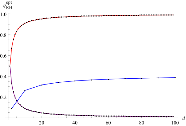
For Hardy paradox with many outcomes we have seen that the paradoxical probability reaches very close to 1 under a generalized no signaling theory. It has great significance. It indicates to the fact that relativistic causality alone does not stop one to demonstrate contradiction with local realism using an argument like (6) with almost $100\%$ success in contrast to the partial success as in quantum case[5, 18].

One can interpret this phenomenon by making two consecutive observations-

Whereas the first observation indicates that the optimal contribution of the ‘paradoxical probability’ connected with complementary events to the total probability of witnessing Hardy nonlocality decreases with increasing local minimal dimension (purple line in Fig.1), the second observation tells that in the asymptotic limit the paradoxical probability corresponding to the argument (6) is equal to PN, which is $1$.

References

- [1] J. S. Bell, Physics 1, 195 (1964).
- [2] J. F. Clauser, M. A. Horne, A. Shimony, and R. A. Holt, Phys. Rev. Lett. 23, 880 (1969).
- [3] D. M. Greenberger, M. A. Horne, A. Zeilinger, in “Bell’s Theorem, Quantum Theory, and Conceptions of the Universe”, M. Kafatos (Ed.), Kluwer, Dordrecht, 69-72 (1989), arXiv:0712.0921v1.
- [4] A. Einstein, B. Podolsky, and N. Rosen, Phys. Rev. 47, 777 (1935).
- [5] L. Hardy, Phys. Rev. Lett. 68, 2981 (1992).
- [6] D. M. Greenberger, M. A. Horne, A. Shimony and A. Zeilinger, Am. J. Phys. 58, 1131 (1990).
- [7] S. Ghosh, G. Kar, and D. Sarkar, Phys. Lett. A 243, 249 (1998); X.-H. Wu and R.-H. Xie, Phys. Lett. A 211, 129 (1996).
- [8] C. Pagonis and R. Clifton, Phys. Lett. A 168, 100-102(1992).
- [9] D. Boschi, S. Branca, F. De. Martini and L. Hardy, Phys. Rev. Lett. 79, 2755 (1997).
- [10] S. Kunkri, and S. K. Choudhary, Phys. Rev. A 72, 022348 (2005).
- [11] K. P. Seshadreesan and S. Ghosh, J. Phys. A: Math. Theor. 44, 315305 (2011).
- [12] R.Rabelo, L.Y.Zhi and V.Scarani, Phys. Rev. Lett. 109, 180401 (2001).
- [13] S.Ghosh, and G.Kar, Phys. Lett. A 240, 191-195(1998).
- [14] S. K. Chudhary, S. Ghosh, G. Kar, S. Kunkri, R. Rahaman, and A. Roy, Quant. Inf. Comp. 10, 0859 (2010).
- [15] T. Fritz, Found. Phys. 41(9), 1493-1501 (2011).
- [16] V. Scarani, N. Gisin, N. Brunner, L. Masanes, S. Pino, and A. Acin, Phys. Rev. A 74, 042339 (2006).
- [17] L. Masanes, A. Acin, and N. Gisin, Phys. Rev. A 73, 012112 (2006).
- [18] J-L. Chen, A. Cabello, Z.P.Xu, H.Y.Su, C. Wu, and L. C. Kwek, Phys. Rev. A 88, 062116 (2013).
- [19] S. Mansfield, PhD Thesis, University of Oxford, 2013.
- [20] R. Rabelo, L. Y. Zhi and V. Scarani, Phys. Rev. Lett. 109, 180401 (2012).
- [21] R. Rahaman, M. G. Parker, P. Mironowicz, M. Pawłowski, arXiv: 1308.6447.
- [22] R. Rahaman, M. Wieśniak, M. Żukowski, arXiv: 1408.1540.
- [23] R. Rahaman, M. Wieśniak, M. Żukowski, arXiv: 1303.0128.
- [24] L. Hardy, Phys. Rev. Lett. 71, 1665 (1993).
- [25] T. F. Jordan, Phys. Rev. A 50, 62 (1994).
- [26] J. Barrett, N. Linden, S. Massar, S. Pironio, S. Popescu, and D. Roberts, Phys. Rev. A 71, 022101 (2005).