High-order Path Integral Monte Carlo methods for solving quantum dot problems

The Path Integral Monte Carlo (PIMC) method remains problemic for solving many-fermion systems due to the “sign” problem. Since the anti-symmetric free-fermion propagator (FFP) is not positive-definite, only its magnitude can be sampled by the Monte Carlo method and observables must then be weighted by the overall sign of all FFP in the path-integral. While a suggested remedy has been proposed[1, 3, 2], the most practical solution in traditional PIMC is to simply side-step the sign-problem by invoking some “fixed-node” or “restricted-path” approximations[4]. Here, we argue that: 1) The sign-problem is not intrinsic to solving a fermion problem; 2) it is only a consequence of a poor approximation to the exact propagator; and 3) it can be automatically minimized by using better, higher-order approximate propagators. By following up on the last point, this work shows that by using optimize fourth-order propagators, accurate results can be obtained for up to 20 spin-polarized electrons in a 2D circular, parabolic quantum dot.

First, let’s dispel the notion that the sign-problem is intrinsic to solving fermion problems in PIMC. If the exact propagator of the system $G({\bf X},{\bf X}^{\prime};\tau)=\langle{\bf X}|{\rm e}^{-\tau H}|{\bf X}^{\prime}\rangle$ is known, then one can compute the energy from

$$E=\frac{\int d{\bf X}HG({\bf X},{\bf X};\tau)}{\int d{\bf X}G(\{{\bf X},{\bf X};\tau)}$$

(1)

without any sign-problem, since $G({\bf X},{\bf X};\tau)>0$. To drive home this point with a non-trivial example, we show in Fig.1, the ground state energies of up to 100 non-interacting fermions in a 2D harmonic oscillator (HO). The exact many-fermion propagator is obtained by generalizing the HO propagator given in Ref.5 to

$$G({\bf X},{\bf X}^{\prime};\tau)=(2\pi\tau C_{T})^{-DN/2}{\rm e}^{-\tau C_{V}\frac{1}{2}\omega^{2}\sum_{i=1}^{N}({\bf x}_{i}^{2}+{\bf x}_{i}^{\prime 2})}\det[{\rm e}^{-\frac{1}{2\tau C_{T}}({\bf x}_{i}-{\bf x}_{j}^{\prime})^{2}}],$$

(2)

where ${\bf X}=\{{\bf x}_{i}\}$, $C_{V}=(\cosh(\omega\tau)-1)/(\sinh(\omega\tau)\omega\tau)$, $C_{T}=\sinh(\omega\tau)/(\omega\tau)$, $D$ is the dimension of ${\bf x}_{i}$ and $N$ is the number of particles. (A proof of this will be given elsewhere, but it is easy to verify that it is exact by a direct calculation, as done here.) Fig.1 demonstrated that this fermion problem can be solved by the Monte Carlo method without any sign-problem and the energy obtained is precisely that of filling the 2D HO energy levels up to the number fermions. (For $N\leq 30$, a single $G({\bf X},{\bf X};\tau)$ is adequate. For larger $N$, Fig.1 uses two propagators $G({\bf X}^{\prime},{\bf X};\tau/2)G({\bf X},{\bf X}^{\prime};\tau/2)>0$. This is because at $\tau=6$, $\tau C_{T}\approx 200$, all entries of the matrix in (2) are nearly one, and the subtraction needed to compute the determinant is beyond Fortran’s double-precision. With two propagators, the needed value of $\tau$ is halved.)

If one tries to approximate this, or any other exact propagator, by a product of primitive action (PA) second-order propagator having one FFP, then one is again confronted by the sign-problem. Since the PA propagator is only accurate at very small time steps, conventionally hundreds of them are needed to extract the ground state at large imaginary times. When one has hundreds of FFP, then whether one is sampling the permuations[4] or directly evaluating the anti-symmetric free-propagator[6], the average of the sign is close to zero and the sign-problem is intractable. This is in spite of the fact that the same problem has just been solve in Fig.1 without any sign-problem. From this perspective, the sign-problem is purely a consequence of a poor approximation to the exact propagator. To the extent that one can better approximate the exact propagator, one can automatically lessen the sign problem. This also means that there is no imperative to “solve” the sign-problem. (Why insist on solving a problem using a poor approximation?) The sign-problem is to be avoided by approximating the exact propagator more accurately using the fewest FFP. If the number of FFP can be kept to less than 10, then one can extract ground state properties before the onset of the sign problem. This is the key idea of this work.

This idea has not been contemplated before because traditional PIMC has been formulated mostly in terms of the low-order, inaccurate PA propagator. It is therefore always deemed impossible to reach the ground state with so few FFP. However, in the bosonic case of liquid helium, we have shown[7] that even a single use of a fourth-order propagator can reach closer to the ground state than many elaborate variational schemes. Recently, the ground state energy of liquid Helium has been computed in PIMC by Sakkos, Casulleras and Boronat[8], using a fourth-order propagator that can be “fine-tuned” to converge at the sixth-order for the energy. Their work reduces, by an order-of-magnitude, the number of propagators (or beads) needed in bosonic PIMC. Subsequently, R. Rota et al.[9] showed that a Ground-State PIMC (GSPIMC) calculation only needed about ten propagators to achieve the same objective! Similar results have also been obtained for the same system with GSPIMC by Zillich, Mayrhofer and Chin[10], using sixth and eighth-order extrapolated propagators. The tremendous sucess of these results have inspired this work to apply higher-order PIMC methods to fermions in quantum dots. Below we will derive fourth-order algorithms for solving a general interacting fermion problem, where the exact HO propagator (2) is not used. (Since the electron repulsion expands the size of the quantum dot, the exact HO propagator is also not effective at strong couplings.)

Aside from using higher-order propagators, the above calculations[7, 9, 10] also computed the energy directly from the Hamiltonian. By the Golden-Thompson inequality[11, 12], the thermodynamic estimator used in conventional PIMC converges to the ground state energy only from below. In the few-propagators case, the thermodynamic estimator is so far from convergence that it is totally useless. The use of the virial estimator is risky for quantum dots, since it may dip below the exact ground state energy[3]. In this work, we follow the success of the GSPIMC method in also using the Hamiltonian estimator in PIMC. This estimator is known[13] in Bosonic PIMC, but we generalize it here to include the anti-symmetric, determinant propagator. There are three advantages in using the Hamiltonian estimator in PIMC. First, it gives a variational upper-bound to the ground state energy, as in GSPIMC. Second, its result can be double-checked by use of a variant, the Clark-Westhaus[14] (CW) form of the kinetic energy. Third, in contrast to GSPIMC, no trial ground-state wave function is needed.

The Hamiltonian for $N$ electrons in a 2D harmonic dot is

$$H=\sum_{i=1}^{N}(-\frac{\hbar^{2}}{2m^{*}}\nabla^{2}_{i}+\frac{1}{2}m^{*}\omega^{2}{\bf r}_{i}^{2})+\sum_{i<j}^{N}\frac{e^{2}}{\kappa|{\bf r}_{i}-{\bf r}_{j}|}.$$

(3)

By expressing ${\bf r}_{i}=\ell_{0}\,{\bf x}_{i}$, where $\ell_{0}=\sqrt{\hbar/(m^{*}\omega)}$ is the harmonic length, one obtains the dimensionless Hamiltonian ${\cal H}$ in terms of dimensionless vectors ${\bf x}_{i}$

$${\cal H}\equiv\frac{H}{\hbar\omega}=\sum_{i=1}^{N}(-\frac{1}{2}\nabla^{2}_{i}+\frac{1}{2}{\bf x}_{i}^{2})+\sum_{i<j}^{N}\frac{\lambda}{|{\bf x}_{i}-{\bf x}_{j}|}$$

(4)

with effective coupling strength $\lambda=\ell_{0}{m^{*}e^{2}}/(\hbar^{2}\kappa)=l_{0}a_{B}^{-1},$ where $a_{B}$ is the effective Bohr radius. The Hamiltonian ${\cal H}$ is the quantum dot’s energy in units of $\hbar\omega$.

The corresponding imaginary time propagator is

$$G(\tau)={\rm e}^{-\beta H/\hbar}={\rm e}^{-\tau{\cal H}}={\rm e}^{-\tau(T+V)},$$

(5)

where $\tau=\beta\omega$ is the dimensionless imaginary time, and $T$ and $V$ are the kinetic and potential operators of ${\cal H}$. The PA propagator approximates $G(\epsilon)$ at small time $\epsilon=\tau/n$ as

$$G_{2}(\epsilon)={\rm e}^{-\epsilon V/2}{\rm e}^{-\epsilon T}{\rm e}^{-\epsilon V/2}+O(\epsilon^{3}),$$

(6)

with coordinate representation

	$\displaystyle G_{2}({\bf X},{\bf X}^{\prime};\epsilon)$	$\displaystyle=$	$\displaystyle\langle{\bf X}|G_{2}(\epsilon)|{\bf X}^{\prime}\rangle$		(7)
		$\displaystyle=$	$\displaystyle{\rm e}^{-\epsilon V({\bf X})/2}G_{0}({\bf X},{\bf X}^{\prime};\epsilon){\rm e}^{-\epsilon V({\bf X}^{\prime})/2},$

where ${\bf X}=\{{\bf x}_{i}\}$ is the position vector of all $N$ fermions, and

$$V({\bf X})=\sum_{i=1}^{N}\frac{1}{2}{\bf x}_{i}^{2}+\sum_{i<j}^{N}\frac{\lambda}{|{\bf x}_{i}-{\bf x}_{j}|}.$$

(8)

The anti-symmetric FFP $G_{0}({\bf X},{\bf X}^{\prime};\epsilon)$ is given by

$$G_{0}({\bf X},{\bf X}^{\prime};\epsilon)=\langle{\bf X}|{\rm e}^{-\epsilon T}|{\bf X}^{\prime}\rangle=(2\pi\epsilon)^{-ND/2}\det{\bf M},$$

(9)

where $N$ is the number of fermions (electrons of the same spin), $D$ is the dimension of the system, and ${\bf M}$ is the $N\times N$ anti-symmetric diffusion matrix

$$M_{ij}({\bf X},{\bf X}^{\prime})=\exp\left[-\frac{1}{2\epsilon}({\bf x}_{i}-{\bf x}^{\prime}_{j})^{2}\right].$$

(10)

For computing the energy, it is convenient to write

	$\displaystyle G_{0}({\bf X},{\bf X}^{\prime};\epsilon)$	$\displaystyle=$	$\displaystyle{\rm e}^{-u_{0}({\bf X},{\bf X}^{\prime};\epsilon)},$
	$\displaystyle u_{0}({\bf X},{\bf X}^{\prime};\epsilon)$	$\displaystyle=$	$\displaystyle\frac{ND}{2}\ln(\epsilon)-\ln(\det{\bf M}).$		(11)

In PIMC, the energy is calculated from (${\bf X}_{k}$ is denoted simply by $k$)

$$E=\frac{\int d1...dnG_{2}(1,2;\epsilon){\cal H}G_{2}(2,3;\epsilon)\cdots G_{2}(n,1;\epsilon)}{\int d1...dnG_{2}(1,2;\epsilon)G_{2}(2,3;\epsilon)\cdots G_{2}(n,1;\epsilon)}$$

(12)

and averaged over all $n$ places where ${\cal H}$ can be inserted between propagators. Since the FFP is not positive-definite, the above integral is sampled as

$$E=\frac{\int d1...dn\ {\rm sgn}E_{\rm H}(k,k+1)P(1,2,\cdots n;\epsilon)}{\int d1...dn\ {\rm sgn}P(1,2,\cdots n;\epsilon)}$$

(13)

with the probability distribution function taken to be

$$P(1,2,\cdots n;\epsilon)=|G_{2}(1,2;\epsilon)G_{2}(2,3;\epsilon)\cdots G_{2}(n,1;\epsilon)|,$$

(14)

and where ${\rm sgn}=\pm 1$ is the overall sign of the product of $G_{2}$’s. The Hamiltonian energy estimator is given by

	$\displaystyle E_{\rm H}({\bf X},{\bf X}^{\prime};\epsilon)=\frac{{\cal H}G_{2}({\bf X},{\bf X}^{\prime};\epsilon)}{G_{2}({\bf X},{\bf X}^{\prime};\epsilon)}$
	$\displaystyle\qquad\qquad=\frac{\sum_{i=1}^{N}(-\frac{1}{2}\nabla^{2}_{i})G_{2}({\bf X},{\bf X}^{\prime};\epsilon)}{G_{2}({\bf X},{\bf X}^{\prime};\epsilon)}+V({\bf X})\ \ \$		(15)

The alternative CW form of the kinetic energy is to let one of the gradient operator acts to the left, giving

			$\displaystyle E_{\rm CW}({\bf X}^{*},{\bf X},{\bf X}^{\prime};\epsilon)$		(16)
		$\displaystyle=$	$\displaystyle\frac{\sum_{i=1}^{N}\frac{1}{2}G_{2}({\bf X}^{*},{\bf X};\epsilon){\mathrel{\mathop{\kern 0.0pt\nabla}\limits^{\leftarrow}}_{i}}\cdot\nabla_{i}G_{2}({\bf X},{\bf X}^{\prime};\epsilon)}{G_{2}({\bf X}^{*},{\bf X};\epsilon)G_{2}({\bf X},{\bf X}^{\prime};\epsilon)}+V({\bf X}).\ \ \ \$

The exact (and the free) propagator satisfies the equation

$$-\frac{\partial}{\partial\epsilon}G({\bf X},{\bf X}^{\prime};\epsilon)={\cal H}G({\bf X},{\bf X}^{\prime};\epsilon).$$

(17)

This equality no longer holds when $G({\bf X},{\bf X}^{\prime};\epsilon)$ is replaced by an approximation, such as $G_{2}({\bf X},{\bf X}^{\prime};\epsilon)$. In this case, when both sides of the equation are divided by $G_{2}({\bf X},{\bf X}^{\prime};\epsilon)$, the RHS gives the “Hamiltonian” estimator as stated above. The LHS then gives the “Thermodynamics” energy estimator

	$\displaystyle E_{\rm TH}({\bf X},{\bf X}^{\prime};\epsilon)=\frac{-\partial_{\epsilon}G_{2}({\bf X},{\bf X}^{\prime};\epsilon)}{G_{2}({\bf X},{\bf X}^{\prime};\epsilon)}$
	$\displaystyle\qquad\qquad=\frac{\partial}{\partial\epsilon}u_{0}({\bf X},{\bf X}^{\prime};\epsilon)+\frac{1}{2}[V({\bf X})+V({\bf X}^{\prime})].\ \ \$		(18)

By the repeated use of the identity

$$\frac{\partial}{\partial\alpha}\ln({\det\bf M})\\ ={\rm Tr}\Bigl[{\bf M}^{-1}\frac{\partial{\bf M}}{\partial\alpha}\Bigr],$$

all three estimators can be computed without difficulties:

	$\displaystyle E_{\rm TH}({\bf X},{\bf X}^{\prime};\epsilon)$	$\displaystyle=$	$\displaystyle\frac{ND}{2\epsilon}-\frac{1}{2\epsilon^{2}}\sum_{i=1}^{N}({\bf x}_{i}^{2}+{{\bf x}_{i}^{\prime}}^{2}-2{\bf x}_{i}\cdot\widetilde{\bf x}_{i}^{\prime})$		(19)
			$\displaystyle\qquad\qquad+\frac{1}{2}[V({\bf X})+V({\bf X}^{\prime})],$

	$\displaystyle E_{\rm H}({\bf X},{\bf X}^{\prime};\epsilon)$	$\displaystyle=$	$\displaystyle\frac{1}{2}\sum_{i=1}^{N}\nabla_{i}^{2}\Bigl[u_{0}+\frac{\epsilon}{2}V\Bigl]$		(20)
			$\displaystyle-\frac{1}{2}\sum_{i=1}^{N}\Bigl[\nabla_{i}(u_{0}+\frac{\epsilon}{2}V)\Bigr]^{2}+V({\bf X}),\ \ \$

	$\displaystyle E_{\rm CW}({\bf X}^{*},{\bf X},{\bf X}^{\prime};\epsilon)=$
	$\displaystyle\frac{1}{2}\sum_{i=1}^{N}\nabla_{i}\Bigl[u_{0}({\bf X},{\bf X}^{*};\epsilon)+\frac{\epsilon}{2}V\Bigr]\cdot\nabla_{i}\Bigl[u_{0}({\bf X},{\bf X}^{\prime};\epsilon)+\frac{\epsilon}{2}V\Bigr]$
	$\displaystyle\qquad\qquad\qquad\qquad\qquad\qquad+V({\bf X}),$		(21)

where

	$\displaystyle\nabla_{i}u_{0}({\bf X},{\bf X}^{\prime};\epsilon)$	$\displaystyle=$	$\displaystyle\frac{1}{\epsilon}({\bf x}_{i}-\widetilde{\bf x}^{\prime}_{i}),$
	$\displaystyle\nabla_{i}^{2}u_{0}({\bf X},{\bf X}^{\prime};\epsilon)$	$\displaystyle=$	$\displaystyle\frac{D}{\epsilon}-\frac{1}{\epsilon^{2}}\Bigl({{\bf x}^{\prime}_{i}}^{2}-\widetilde{{\bf x}}_{i}^{\prime 2}\Bigr).$		(22)

and where $\widetilde{\bf x}^{\prime}_{i}$ is defined by

$$\widetilde{\bf x}^{\prime}_{i}\equiv\sum_{k=1}^{N}{\bf x}^{\prime}_{k}M_{ik}({\bf X},{\bf X}^{\prime})M^{-1}_{ki}({\bf X},{\bf X}^{\prime}).$$

(23)

Thus in all three energy estimates, the calculation of ${\bf M}^{-1}$ is required. In the free propagator case, one has indeed $E_{\rm TH}=E_{\rm H}$. The CW estimator will generally have greater variance than the Hamiltonian estimator.

After a set of $M$ configureations $\{{\bf X}_{i}^{(m)}\}$ has been generated according to $P({\bf X}_{1},{\bf X}_{2},\cdots{\bf X}_{n};\epsilon)$, the energy can be computed by using the above three estimators as

$$E=\frac{\sum_{m=1}^{M}{\rm sgn}_{k}[\frac{1}{n}\sum_{k=1}^{n}E_{\rm H,CW,TH}({\bf X}_{k}^{(m)},{\bf X}_{k+1}^{(m)};\epsilon)]}{\sum_{k=1}^{M}{\rm sgn}_{k}}.$$

(24)

For $N=8$ spin-polarized electrons at the strong-coupling limit of $\lambda=8$, the the energy of these three estimators are compared in Fig.2. This is the largest quantum dot at the strongest coupling considered in Egger et al.’s PIMC calculation[3] and in Rontani et al.’s configuration-interaction study[15]. The thermodynamics estimator showed no convergence for up to 8 PA propagators, whereas the Hamiltonian and CW estimators are in excellent agreement in providing upper-bounds to the ground state energy from 2 to 8 propagators. The sign problem is completely under control in these calculations. The Hamiltonian energy minimum in the 8 propagators case is already close to the result of Egger et al.[3]. This strongly suggests that improving the propagator beyond second-order can circumvent the sign problem in these quantum dot calculations.

The short-time propagator can be approximated to any order by a product decomposition,

$${\rm e}^{-\epsilon(T+V)}=\prod_{i=1}^{n}{\rm e}^{-t_{i}\epsilon T}{\rm e}^{-v_{i}\epsilon V},$$

(25)

with a suitable set of coefficients $\{t_{i},v_{i}\}$. However, as first shown by Sheng[16], Suzuki[17], Goldman-Kaper[18], and more recently in a constructive proof by Chin[19], beyond second order, any factorization of the form (25) must contain some negative coefficients in the set $\{t_{i},v_{i}\}$ and cannot be used in PIMC. This is because if $t_{i}$ were negative, then replacing $\epsilon\rightarrow t_{i}\epsilon$ in the free fermion propagator (10) would result in an unbounded function that cannot be normalized as a probability. This simply reflects the fact that diffusion is a time-irreversible process. To have forward fourth-order schemes, with all positive coefficients, one must include the gradient potential

$$[V,[T,V]]=\sum_{i=1}^{N}|\nabla_{i}V|^{2},$$

(26)

in the decomposing process[20, 21]. These fourth-order schemes have been used successfully in bosonic DMC and PIMC simulations[22, 23, 8, 9]. Here, we will use a more extended family of these forward fourth-order propagators, with arbitrary numbers of free-fermion $T$ operators as described in Refs.19, 24.

In order to compare with the PA algorithm, we will characterize these algorithms by their number of $T$ operators, or beads. We will consider approximations of the form (25) with $t_{1}=0$ and with left-right symmetric coefficients $v_{1}=v_{N}$, $t_{2}=t_{N}$, etc.,

$\displaystyle{\cal T}_{(N-1)B}^{(4)}(\epsilon)$

$\displaystyle=$

$\displaystyle{\rm e}^{v_{1}\epsilon V}{\rm e}^{t_{2}\epsilon T}{\rm e}^{v_{2}\epsilon V}\cdots{\rm e}^{t_{N}\epsilon T}{\rm e}^{v_{N}\epsilon V}.$

(27)

This will be fourth-order if one chooses $\{t_{i}\}>0$ with $\sum_{i=1}^{N}t_{i}=1$, fixes $\{v_{i}\}$ by

$$v_{1}=v_{N}=\frac{1}{2}+\lambda_{2}(1-t_{2}),\quad v_{i}=-\lambda_{2}(t_{i}+t_{i+1}),$$

(28)

where $\lambda_{2}=-\phi^{-1}/2$, $\ \phi=1-\sum_{i=1}^{N}t_{i}^{3}$, and divide the required gradient potential term

$$\frac{1}{24}(\frac{1}{\phi}-1)\epsilon^{3}[V,[T,V]]$$

(29)

left-right symmetrically among all the $v_{i}\epsilon V$ terms in (27). In order to compute the Hamiltonian energy as simply as in the PA case (with only minor changes from $\epsilon\rightarrow t_{i}\epsilon$ and $\epsilon\rightarrow v_{i}\epsilon$), the gradient potential term must not be distributed to the $v_{1}$ and $v_{N}$ potential terms. Because of this constraint, there is no free parameter in the 2-bead calculation (algorithm 4A of Ref.21) that can be used to optimized the energy. Similarily, the Takahashi and Imada fourth-order trace propagator[6] cannot be used, becuase it is difficult to compute the Hamiltonian estimator with the gradient potential. The freedom to choose $\{t_{i}\}$ and to distribute the the gradient potential terms among the remaining $v_{i}$ potential terms then allows one to fine-tune the propagator to minimize the energy[8, 9].

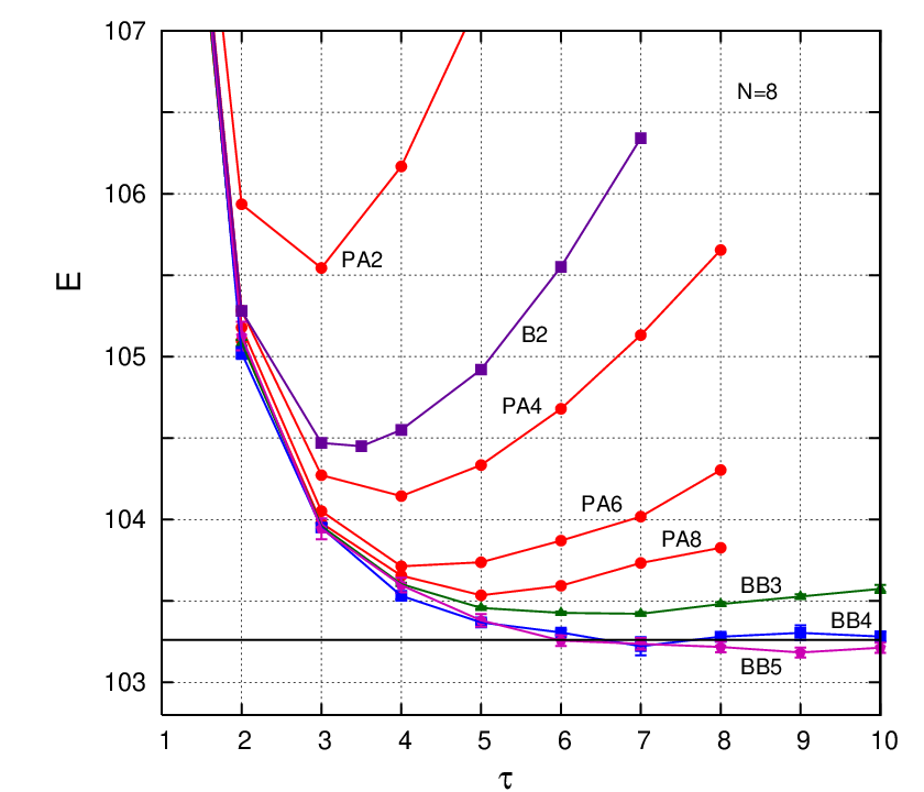
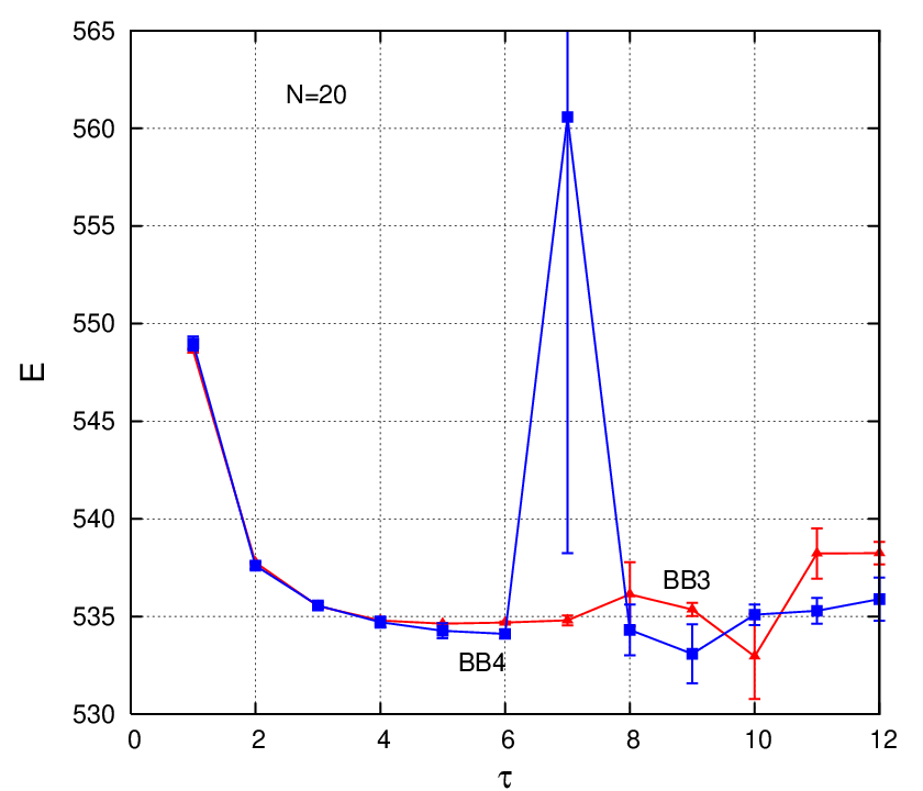
In Fig.3 we compare the Hamiltonian energy obtained by these optimized fourth-order propagator with those of the PA propagator in Fig.2. The energy is computed by sampling the trace of only a single fourth-order propagator having 2 to 5 beads. The 2-bead case, even without optimization, is substantially better than PA2. The optimized 3-bead case has energy lower than that of 8 PA propagators. The 5-bead case has energy lower than that of Egger et al.’s calculation[3]. As the calculation becomes more accurate with increasing number of beads, $E(\tau)$ levels off in approaching the exact result, as in Fig.1, but still retains a shallow minimum. Table 1 compares our results to those obtained by the PIMC method of Egger et al.[3], the configuration-interaction method of Rontani et al.[15] and the Diffusion Monte Carlo (DMC) method of F. Pederiva et al.[25] and Ghosal et al.[26], for up to $N\approx 20$ spin-polarized electrons. In the case of 2 and 3 beads, results can be obtained up to $N=30$ and $N=25$ respectively. These calculations were done on a laptop computer and each entry can take up to $\approx 2-3$ days. Entries requiring longer running time were left undone. Substantial improvements are expected when the code is ported supercomputers. In Fig.4, we show the convergence of the 3 and 4-bead propagators for solving the case of $N=20$ spin-polarized electrons. This is a good illustration of the sudden appearance of the sign problem, which blew up the 4-bead calculation with a large variance at $\tau=7$. Nevertheless, the Hamiltonian estimator still gives excellent upper-bounds to the energy at $\tau=6$ and $\tau=8$.

In this work, we have shown that optimized fourth-order propagators, in using only 3-5 FFP, together with the use of the Hamiltonian estimator, can effectively limit the severity of the sign problem and allow accurate calculation of quantum dot energies for up 20 fermions. The 2-bead calculations are about 1% too high, but they are without the sign-problem and can be used as a quick variational estimate at $N$ much larger than 20.

I thank my colleague Eckhard Krotscheck for hospitality and support at Linz, Austria during the summers of 2010-2012, when this work was initiated. This publication was made possible by NPRP GRANT #5-674-1-114 from the Qatar National Research Fund (a member of Qatar Foundation).

References

- [1] C. H. Mak, R. Egger, and H. Weber-Gottschick, Phys. Rev. Lett. 81, 4533 (1998).
- [2] R. Egger, L. Mühlbacher, and C. H. Mak, Phys. Rev. E 61, 5961 (2000).
- [3] R. Egger, W. Häusler, C. H. Mak and H. Grabert, Phys. Rev. Lett. 82, 3320 (1999); 83, 462(E) (1999).
- [4] D. M. Ceperley, Rev. Mod. Phys., 67, 279 (1995).
- [5] S. A. Chin and E. Krotscheck, Phys. Rev. E 72, 036705 (2005).
- [6] M. Takahashi and M. Imada, J. Phys. Soc. Jpn 53, 3765 (1984).
- [7] Orion Ciftja and Siu A. Chin, Phys. Rev. B 68,134510 (2003)
- [8] K. Sakkos, J. Casulleras, and J. Boronat, J. Chem. Phys. 130, 204109 (2009)
- [9] R. Rota, J. Casulleras, F. Mazzanti, and J. Boronat, Phys. Rev. E 81, 016707 (2010)
- [10] R. E. Zillich, J. M. Mayrhofer and Siu A. Chin, J. Chem. Phys. 132, 044103 (2010).
- [11] S. Golden, Phys. Rev. 127, B1127, (1965).
- [12] C. J. Thompson, J. Math. Phys. 6, 1812 (1965).
- [13] T. W. Whitfield and G. L. Martyna, J. Chem. Phys. 132, 044103 (2010).
- [14] J. W. Clark, in Progress in Particle and Nuclear Physics, Vol. II, edited by D. H. Wilkinson (Pergamon, Oxford, 1979), and references cited therein.
- [15] M. Rontani, C. Cavazzoni, D. Bellucci and G. Goldoni J. Chem. Phys. 124, 124102 (2006).
- [16] Q. Sheng, IMA J. Num. Anaysis, 9, 199 (1989).
- [17] M. Suzuki, J. Math. Phys. 32, 400 (1991).
- [18] D. Goldman and T. J. Kaper, SIAM J. Numer. Anal., 33, 349 (1996).
- [19] S. A. Chin, Phys. Lett. A 354, 373 (2006)
- [20] M. Suzuki, Computer Simulation Studies in Condensed Matter Physics VIII, eds, D. Landau, K. Mon and H. Shuttler (Springler, Berlin, 1996).
- [21] S. A. Chin, Phys. Lett. A 226, 344 (1997).
- [22] H. A. Forbert and S. A. Chin, Phys. Rev. E 63, 016703 (2001); Phys. Rev. B 63, 144518 (2001).
- [23] S. Jang, S.Jang and G. A. Voth, J. Chem. Phys. 115 7832, (2001).
- [24] S. A. Chin, Phys. Rev. E, 73, 026705 (2006).
- [25] F. Pederiva, C.J. Umrigar and E. Lipparini, Phys. Rev. B 62, 8120 (2000), B 68, 089901(E) (2003)
- [26] A. Ghosal, A. D. Güclü, C. J. Umrigar, D. Ullmo and H. U. Baranger Phys. Rev. B 76, 085341 (2007)