跳到论文正文
W Papers独立论文阅读器 arXiv:1411.6544 论文正文 计算阅读时间 · 0%
引用这篇论文根据当前论文元数据生成,正式投稿前建议核对。


License: arXiv.org perpetual non-exclusive license
arXiv:1411.6544v2 [cond-mat.quant-gas] 10 Mar 2015

A variational approach to repulsively interacting three-fermion systems in a one-dimensional harmonic trap

N. J. S. Loft Affiliation: Department of Physics and Astronomy, Aarhus University, DK-8000 Aarhus C, Denmark    A. S. Dehkharghani Affiliation: Department of Physics and Astronomy, Aarhus University, DK-8000 Aarhus C, Denmark    N. P. Mehta Affiliation: Department of Physics and Astronomy, Trinity University, San Antonio, Texas, USA    A. G. Volosniev Affiliation: Institut für Kernphysik, Technische Universität Darmstadt, 64289 Darmstadt, Germany Affiliation: Department of Physics and Astronomy, Aarhus University, DK-8000 Aarhus C, Denmark    N. T. Zinner Affiliation: Department of Physics and Astronomy, Aarhus University, DK-8000 Aarhus C, Denmark
August 24, 2026
Abstract

We study a three-body system with zero-range interactions in a one-dimensional harmonic trap. The system consists of two spin-polarized fermions and a third particle which is distinct from two others (2+1 system). First we assume that the particles have equal masses. For this case the system in the strongly and weakly interacting limits can be accurately described using wave function factorized in hypercylindrical coordinates. Inspired by this result we propose an interpolation ansatz for the wave function for arbitrary repulsive zero-range interactions. By comparison to numerical calculations, we show that this interpolation scheme yields an extremely good approximation to the numerically exact solution both in terms of the energies and also in the spin-resolved densities. As an outlook, we discuss the case of mass imbalanced systems in the strongly interacting limit. Here we find spectra that demonstrate that the triply degenerate spectrum at infinite coupling strength of the equal mass case is in some sense a singular case as this degeneracy will be broken down to a doubly degenerate or non-degenerate ground state by any small mass imbalance.

I Introduction

Recent advances in cold atomic gas experiments has made it possible to work with microscopic system sizes for fermionic [1, 2, 3, 4] and bosonic samples [5, 6, 7, 8]. Furthermore, by application of optical lattices [9] and use of Feshbach resonances [10] it is possible to tune both the geometry and the interaction strength of these setups. This allows the cold atom systems to address a host of interesting physical models in lower spatial dimensions that are typically not so easily accessible in other fields. In particular, when the system is squeezed down to a regime where particles effectively move along just a single spatial direction, one can hope to realize some of the exactly solvable models that are known for both few- and many-body systems in one dimension (1D) [11, 12]. About a decade ago this hope led to the realization of the strongly repulsive (hard-core) Bose gas [13, 14, 15] in the so-called Tonks-Girardeau regime [16, 17, 18] and later on also to the so-called super-Tonks-Girardeau gas [19] which is an excited state for strong attractive interactions [20]. More recently, the strongly repulsive and attractive regimes have been explored with few-body systems of two-component fermions [2, 3, 4] and these recent experimental developments provide a major motivation for the current work.

The experimental progress has generated great interest for few-body problems in one-dimensional geometries for both bosonic [21, 22, 23, 24, 25, 26, 27, 28], fermionic [29, 30, 31, 32, 33, 34, 35, 36, 37, 38, 39, 40, 41, 42, 43, 44, 45, 46], and mixed systems [47, 48, 49, 50, 51, 52, 53, 54, 55, 56, 57, 58, 59, 60, 61]. Recently, it has been shown that for strong short-range repulsive interactions a 1D two-component Fermi system in a harmonic trap exhibits strong magnetic correlations already at the three-body level [37, 40]. More generally, one finds that in the ground state of strongly interacting N+1N+1 system the impurity will be mainly observed in the middle of the trap [40, 46]. This result can be generalized to other types of 1D confinement [39, 42]. This should be contrasted to two-component bosonic systems with equal strength intra- and interspecies interactions where the ground state for strong repulsion will be the one predicted by Girardeau [24] and the impurity would be essentially delocalized [39]. In the present paper we seek further analytical and semi-analytic insights into the 1D fermionic three-body problem in a harmonic trap by constructing a class of variational wave functions for arbitrary repulsive zero-range interaction strength. Relying on our knowledge developed for the weakly and strongly interacting limits we provide and study a variational wave function of the three-body problem that connects these two limits. By comparison to numerical results we show that our class of states yields an exceptionally good approximation for the low-energy part of the energy spectrum and also gives very accurate spin-resolved densities. This shows that intuitive approaches at the level of the wave function shape are effective in strongly interacting 1D few-fermion systems. For related recent work on single-component bosons see Refs. [25, 27] and for recent work on the two-component three-body bosonic system see Ref. [61]. As an outlook we consider the 2+1 system in the case where the masses are imbalanced and find an intriguing change in the ground state structure for strong interactions which occurs for any infinitesimal difference in the masses between the two components. Our results indicate that the large degeneracy of strongly interacting two-component systems is in some sense accidental and that spectrum for equal masses is in fact a special case (although of course an extremely important one).

The paper is organized as follows. In section II we introduce the system, our choice of coordinates and discuss the symmetries of our Hamiltonian. In section III we solve the problem for zero and infinite zero-range interaction strength while the variational approach to arbitrary repulsive interaction strength is discussed in Section IV. In Section V we provide an outlook towards the case where the two components have unequal masses by solving the general problem in the strongly interacting regime. Section VI contains our conclusions and outlook. Finally, we provide three appendices with technical details of important derivations discussed in the main text.

II The system

In this section, we introduce the system that will be the subject for the rest of the article. The section is largely based on reference [52] and is mainly concerned with different coordinate systems in which the system can be described. At the end of this section we discuss the parity and permutation symmetries of the Hamiltonian.

II.1 The Hamiltonian and coordinate transformations

Consider the Hamiltonian for a system of NN particles in one dimension

H=H0+VH=H_{0}+V

consisting of a harmonic trap Hamiltonian

H0=∑i=1N(p~i22​mi+mi​ω22​q~i2)H_{0}=\sum\limits_{i=1}^{N}\left(\frac{{\tilde{p}_{i}}^{2}}{2m_{i}}+\frac{m_{i}\,\omega^{2}}{2}{\tilde{q}_{i}}^{2}\right) (1)

and an interaction term

V=∑i=1N−1∑i<jNgi​j​δ​(q~i−q~j),V=\sum\limits_{i=1}^{N-1}\,\sum\limits_{i<j}^{N}\,g_{ij}\,\delta\!\left(\tilde{q}_{i}-\tilde{q}_{j}\right)\;, (2)

where q~i\tilde{q}_{i} and p~i=−i​ℏ​(∂/∂q~i)\tilde{p}_{i}=-i\hbar(\partial/\partial\tilde{q}_{i}) are correspondingly the position and momentum operators of particle ii, and mim_{i} is its mass. The first part (1) describes NN such particles in a harmonic oscillator potential with angular frequency ω\omega. The second part (2), containing Dirac’s delta functions, describes a contact interaction between particles ii and jj of strength gi​jg_{ij}.

In this article everywhere except section V, we shall limit ourselves to N=3N=3, m1=m2=m3≡mm_{1}=m_{2}=m_{3}\equiv m, and g13=g23≡g≥0g_{13}=g_{23}\equiv g\geq 0. That is, we first consider a system of three particles of equal mass. We take particles 1 and 2 to be spinless (spin-polarized) fermions interacting with the third particle with strength gg. Due to the Pauli principle the wave function should vanish whenever particles 1 and 2 meet, thus the corresponding contribution from the delta function interaction should be neglected. Having this in mind we assume g12=0g_{12}=0 to simplify notation.

Also, we introduce the length scale σ=ℏ/m​ω\sigma=\sqrt{\hbar/m\omega} such that more convenient dimensionless coordinates can be defined as

qi=q~iσandpi=p~i​σℏ.q_{i}=\frac{\tilde{q}_{i}}{\sigma}\quad\text{and}\quad p_{i}=\frac{\tilde{p}_{i}\,\sigma}{\hbar}\;.

In these coordinates the Hamiltonian of the three particle system becomes

H0=ℏ​ω2​∑i=13(pi2+qi2),H_{0}=\frac{\hbar\omega}{2}\sum\limits_{i=1}^{3}\left({p_{i}}^{2}+{q_{i}}^{2}\right)\;, (3)
V=gσ​δ​(q1−q3)+gσ​δ​(q2−q3).V=\frac{g}{\sigma}\,\delta\!\left(q_{1}-q_{3}\right)+\frac{g}{\sigma}\,\delta\!\left(q_{2}-q_{3}\right)\;. (4)

Now we choose units such that ℏ≡ω≡m≡1\hbar\equiv\omega\equiv m\equiv 1, then it follows that also σ=1\sigma=1. It is possible to separate the center-of-mass motion and the relative motion of the particles if we define a new set of coordinates 𝐫≡[x,y,z]T\mathbf{r}\equiv[x,y,z]^{T} by applying a linear transformation to 𝐪≡[q1,q2,q3]T\mathbf{q}\equiv[q_{1},q_{2},q_{3}]^{T} given by the matrix 𝐉\mathbf{J}, that is

𝐫=𝐉𝐪or[xyz]=[12−1201616−23131313]​[q1q2q3].\mathbf{r}=\mathbf{J}\mathbf{q}\quad\text{or}\quad\begin{bmatrix}x\\[5.0pt] y\\[5.0pt] z\end{bmatrix}=\begin{bmatrix}\frac{1}{\sqrt{2}}&-\frac{1}{\sqrt{2}}&0\\[5.0pt] \frac{1}{\sqrt{6}}&\frac{1}{\sqrt{6}}&-\frac{\sqrt{2}}{\sqrt{3}}\\[5.0pt] \frac{1}{\sqrt{3}}&\frac{1}{\sqrt{3}}&\frac{1}{\sqrt{3}}\end{bmatrix}\begin{bmatrix}q_{1}\\[5.0pt] q_{2}\\[5.0pt] q_{3}\end{bmatrix}\;. (5)

The new coordinates, (x,y,z)(x,y,z), are called the standard normalized Jacobi coordinates. Since 𝐉T​𝐉=𝟏\mathbf{J}^{T}\mathbf{J}=\mathbf{1} is the identity matrix and det𝐉=1\det\mathbf{J}=1, the matrix 𝐉\mathbf{J} is a member of the three dimensional rotation group SO​(3)\text{SO}(3). Therefore 𝐫\mathbf{r} is merely a rotation of 𝐪\mathbf{q} and the norm of the vector is conserved, i.e. 𝐫2=𝐪2\mathbf{r}^{2}=\mathbf{q}^{2}. Since 𝐉−1=𝐉T\mathbf{J}^{-1}=\mathbf{J}^{T}, the inverse relation is given by 𝐪=𝐉T​𝐫\mathbf{q}=\mathbf{J}^{T}\mathbf{r}. As is seen from eq. (5), zz describes the center-of-mass position of the system since all individual positions of the particles are weighted equally. The relative motion is described with coordinates xx and yy, as visualized in figure 1.

Refer to caption
Figure 1: The coordinates xx and yy describe the relative position of the particles as opposed to q1q_{1}, q2q_{2} and q3q_{3} describing the absolute positions. The illustration shows the scaled coordinates 2​x=q1−q2\sqrt{2}\,x=q_{1}-q_{2} and 62​y=12​(q1+q2)−q3\tfrac{\sqrt{6}}{2}\,y=\tfrac{1}{2}\left(q_{1}+q_{2}\right)-q_{3}, the latter pointing from q3q_{3} to the center-of-mass coordinate of the particle 1 and 2 subsystem. Particle 1 and 2 are indistinguishable, but distinguishable from particle 3, like for instance two spin-up particles vs. one spin-down.

Similarly, we rotate the momenta coordinates, 𝐩\mathbf{p}, such that 𝐤=𝐉𝐩\mathbf{k}=\mathbf{J}\mathbf{p}, where 𝐤2=−∇𝐫2\mathbf{k}^{2}=-{\mbox{\boldmath$\nabla$}_{\mathbf{r}}}^{2} – the subscript 𝐫\mathbf{r} denotes that the differentiation is done with respect to the 𝐫\mathbf{r}-coordinate system. In the Jacobi coordinates, the two terms of the Hamiltonian become

H0\displaystyle H_{0} =12​(𝐫2−∇𝐫2)\displaystyle=\frac{1}{2}\left(\mathbf{r}^{2}-{\mbox{\boldmath$\nabla$}_{\mathbf{r}}}^{2}\right)
=12​(x2−∂2∂x2+y2−∂2∂y2+z2−∂2∂z2),\displaystyle=\frac{1}{2}\left(x^{2}-\frac{\partial^{2}}{\partial x^{2}}+y^{2}-\frac{\partial^{2}}{\partial y^{2}}+z^{2}-\frac{\partial^{2}}{\partial z^{2}}\right)\;, (6)
V=g2​[δ⁡(−12​x+32​y)+δ⁡(−12​x−32​y)].V=\frac{g}{\sqrt{2}}\,\Bigg[\delta\!\left(-\tfrac{1}{2}x+\tfrac{\sqrt{3}}{2}y\right)+\delta\!\left(-\tfrac{1}{2}x-\tfrac{\sqrt{3}}{2}y\right)\Bigg]\;. (7)

Notice that H0H_{0} is identical to the Hamiltonian for a single particle at position 𝐫\mathbf{r} in a three dimensional harmonic oscillator. It is clearly separable in all of its coordinates, and each term has the well-known energy eigenbasis of a one dimensional harmonic oscillator. However, the interaction term, VV, is not separable in its coordinates, fortunately it only depends on xx and yy, so the total Hamiltonian, HH, can be separated in terms of the center-of-mass motion (zz-direction) and relative motion (x​yxy-plane). Since the relative motion of the particles belongs to the x​yxy-plane, we define one last set of coordinates to get the most beneficial description of this plane:

ρ=x2+y2,ρ∈[0,∞[;\displaystyle\rho=\sqrt{x^{2}+y^{2}}\;,\quad\rho\in[0,\infty[\;;
tanϕ=yx,ϕ∈[−π,π[.\displaystyle\tan\phi=\frac{y}{x}\;,\quad\phi\in[-\pi,\pi[\;.

The set (ρ,ϕ,z)(\rho,\phi,z) is called the Jacobi hypercylindrical coordinates. The trap potential and the interaction potential take the form

H0=12​(z2−∂2∂z2+ρ2−1ρ​∂∂ρ−∂2∂ρ2−1ρ2​∂2∂ϕ2),H_{0}=\frac{1}{2}\left(z^{2}-\frac{\partial^{2}}{\partial z^{2}}+\rho^{2}-\frac{1}{\rho}\frac{\partial}{\partial\rho}-\frac{\partial^{2}}{\partial\rho^{2}}-\frac{1}{\rho^{2}}\frac{\partial^{2}}{\partial\phi^{2}}\right)\;, (8)
V=g2​ρ​[δ⁡(ϕ−π6)+δ⁡(ϕ+5​π6)+δ⁡(ϕ+π6)+δ⁡(ϕ−5​π6)].V=\frac{g}{\sqrt{2}\,\rho}\Big[\delta\!\left(\phi-\tfrac{\pi}{6}\right)+\delta\!\left(\phi+\tfrac{5\pi}{6}\right)+\delta\!\left(\phi+\tfrac{\pi}{6}\right)+\delta\!\left(\phi-\tfrac{5\pi}{6}\right)\Big]\;. (9)

In figure 2 we show the relative configuration space for the particles, which will become helpful when we describe the wave function in the following sections. By relative configuration space we mean that any relative configuration of the three particles is uniquely determined by a single point in the plane, this point being given in either (x,y)(x,y) or (ρ,ϕ)(\rho,\phi) coordinates. To include all absolute configurations, we would need to include a third dimension, namely the zz-axis, since this determines the center-of-mass position. The solid lines on the figure represent two particles sharing the same position. Since we assume a contact interaction between two distinguishable particles the delta functions in eq. (9) are non-zero only on the solid lines q2=q3q_{2}=q_{3} and q1=q3q_{1}=q_{3}.

Refer to caption
Figure 2: The relative configuration space showing all possible ways to order the three particles relative to each other. Thinking of spin 12\tfrac{1}{2} particles, we could take particle 1 and 2 to be in the spin-up state and particle 3 to be in the spin-down state, and these spin configurations are also depicted.

II.2 Parity and permutation symmetry

From (3) and (4) we see that the total Hamiltonian is invariant under a simultaneous change of sign in all spatial coordinates. If Π\Pi denotes the parity operator transforming qi↦−qiq_{i}\mapsto-q_{i} for every i∈{1,2,3}i\in\{1,2,3\}, then surely [H,Π]=0\left[H,\Pi\right]=0. In the Jacobi coordinates the parity transformation is (x,y,z)↦(−x,−y,−z)(x,y,z)\mapsto(-x,-y,-z), and so the parity operator can be decomposed as Π=Πx​y+Πz\Pi=\Pi_{xy}+\Pi_{z}, where the first term acts only on coordinates in the relative x​yxy-plane and the last term acts only the coordinate on the zz-axis. We choose this decomposition because the Hamiltonian is separable in the same way. From (6) and (7) [H,Πz]=0\left[H,\Pi_{z}\right]=0, and then [H,Π]=[H,Πx​y]+[H,Πz]=[H,Πx​y]=0\left[H,\Pi\right]=\left[H,\Pi_{xy}\right]+\left[H,\Pi_{z}\right]=\left[H,\Pi_{xy}\right]=0. From now on the term parity will refer to Πx​y\Pi_{xy}.

By construction the Hamiltonian is invariant under the exchange of particles 1 and 2. It immediately follows that [H,P12]=0\left[H,P_{12}\right]=0 where P12P_{12} denotes the permutation operator exchanging the coordinates of particles 1 and 2. Since the transformation x↦−xx\mapsto-x is equivalent to q1↔q2q_{1}\leftrightarrow q_{2}, the Pauli principle is satisfied if and only if the wave function fulfills ψ⁡(−x,y,z)=−ψ⁡(x,y,z)\psi(-x,y,z)=-\psi(x,y,z). One obvious consequence is that the wave function must vanish on the yy-axis in figure 2.

We easily verify that [Πx​y,P12]=0\left[\Pi_{xy},P_{12}\right]=0, and that HH, Πx​y\Pi_{xy} and P12P_{12} are all hermitian. Therefore we may find a basis that is simultaneously described by energy, parity and permutation of particles 1 and 2. The eigenvalues for both the parity operator and the permutation operator are ±1\pm 1. However, the Pauli principle states that only eigenfunctions with the eigenvalue −1-1 for P12P_{12} are valid wave functions (the eigenvalue +1+1 is only for bosonic wave functions as discussed in Refs. [52, 61]). We say that the states with parity eigenvalue +1+1 have even parity, and the states with −1-1 have odd parity. Thus we require

ψ⁡(−x,y,z)=−ψ⁡(x,y,z)\displaystyle\psi(-x,y,z)=-\psi(x,y,z) (Pauli principle)
ψ⁡(−x,−y,z)=±ψ⁡(x,y,z)\displaystyle\psi(-x,-y,z)=\pm\psi(x,y,z) (even/odd parity)

III The interaction limits

In this section, we find the exact wave functions that solve the Schrödinger equation at g=0g=0 and 1/g=01/g=0.

III.1 Non-interacting limit, g=0g=0

Without the interaction the system can be considered as a three-dimensional quantum harmonic oscillator with Hamiltonian H0H_{0}. Here we write down the eigenspectrum of this textbook Hamiltonian using (ρ,ϕ,z)(\rho,\phi,z) coordinates. If we denote an energy eigenbasis of H0H_{0} in this set of coordinates by |ν,μ,η⟩\left|\nu,\mu,\eta\right>, we separate the center-of-mass motion and the relative motion as |ν,μ,η⟩=|ν,μ⟩⊗|η⟩\left|\nu,\mu,\eta\right>=\left|\nu,\mu\right>\otimes\left|\eta\right>. The wave functions for the center-of-mass motion are the eigenstates of the one dimensional harmonic oscillator, i.e.

⟨z|η⟩\displaystyle\left<z\,\right|\left.\!\eta\right> =ψη​(z)\displaystyle=\psi_{\eta}(z)
=π−1/42η​η!e−z2/2Hη(z),η=0,1,2,…\displaystyle=\frac{\pi^{-1/4}}{\sqrt{2^{\eta}\eta!}}\,e^{-z^{2}/2}\,H_{\eta}(z)\;,\quad\eta=0,1,2,\dots (10)

where Hη​(z)H_{\eta}(z) denotes the Hermite polynomial of degree η\eta. The relative motion is described with functions11 1 Due to the Pauli principle it is impossible to have μ=0\mu=0.

⟨ρ,ϕ|ν,μ⟩\displaystyle\left<\rho,\phi\right|\left.\!\nu,\mu\right> =ψν,μ​(ρ,ϕ)\displaystyle=\psi_{\nu,\mu}(\rho,\phi)
=A⋅Lν(μ)(ρ2)e−ρ2/2ρμf(μ,ϕ),\displaystyle=A\cdot L_{\nu}^{(\mu)}\!\big(\rho^{2}\big)\,e^{-\rho^{2}/2}\,\rho^{\mu}\,f(\mu,\phi)\;, (11)
ν=0,1,2,…andμ=1,2,3​…,\displaystyle\;\nu=0,1,2,\dots\quad\text{and}\quad\mu=1,2,3\dots\;,

where AA is a normalization constant, Lν(μ)​(ρ2)L_{\nu}^{(\mu)}\!\big(\rho^{2}\big) denotes the associated Laguerre polynomial and f⁡(μ,ϕ)f(\mu,\phi) contains the angular dependency of the wave function and is in the simultaneous energy and parity eigenbasis either equal to sin⁡(μ​ϕ)\sin(\mu\phi) or cos⁡(μ​ϕ)\cos(\mu\phi) (see below). However, we keep the general notation for the angular function f⁡(μ,ϕ)f(\mu,\phi). Since Lν(μ)​(ρ2)L_{\nu}^{(\mu)}\!\big(\rho^{2}\big) have ν\nu roots, this is the quantum number determining the number of roots in the radial ρ\rho-direction and thus we refer to ν\nu as a radial excitation quantum number. Also we note that the value of μ\mu determines the number of roots in the angular ϕ\phi-direction, and so we regard μ\mu as an angular excitation quantum number. The quantum number for the center-of-mass excitation is η\eta. The energy corresponding to these quantum numbers is given as

E=⟨ν,μ,η|H0|ν,μ,η⟩=32+2ν+μ+η.E=\left<\nu,\mu,\eta\vphantom{H_{0}}\right|H_{0}\left|\nu,\mu,\eta\vphantom{H_{0}}\right>=\tfrac{3}{2}+2\nu+\mu+\eta\;. (12)

III.2 Impenetrable regime, 1/g=01/g=0

As discussed in the previous section, the center-of-mass motion is separable for all values of gg, and so we will focus on the wave function describing the relative motion. To start the discussion we first derive conditions for the wave function on the lines of interaction in figure 2. Let ϕ0∈{±π6,±5​π6}\phi_{0}\in\big\{\pm\tfrac{\pi}{6},\pm\tfrac{5\pi}{6}\big\}, we then integrate the time-independent Schrödinger equation, H​ψ=E​ψH\psi=E\psi, in the ε\varepsilon-neighborhood of ϕ0\phi_{0} and let ε→0\varepsilon\rightarrow 0:

−12​ρ2limε→0∫ϕ0−εϕ0+εdϕ∂2∂ϕ2ψ(ρ,ϕ)\displaystyle-\frac{1}{2\rho^{2}}\lim\limits_{\varepsilon\rightarrow 0}\int\limits_{\phi_{0}-\varepsilon}^{\phi_{0}+\varepsilon}\mathrm{d}\phi\,\frac{\partial^{2}}{\partial\phi^{2}}\psi(\rho,\phi)
+g2​ρlimε→0∫ϕ0−εϕ0+εdϕδ(ϕ0−ϕ)ψ(ρ,ϕ)=0\displaystyle+\frac{g}{\sqrt{2}\,\rho}\lim\limits_{\varepsilon\rightarrow 0}\int\limits_{\phi_{0}-\varepsilon}^{\phi_{0}+\varepsilon}\mathrm{d}\phi\,\delta\!\left(\phi_{0}-\phi\right)\,\psi(\rho,\phi)=0

All other terms vanish due to the continuity of the wave function. The remaining integrals yield

−12​ρ2limε→0(∂ψ∂ϕ|ϕ0+ε−∂ψ∂ϕ|ϕ0−ε)+g2​ρψ(ρ,ϕ0)=0.-\frac{1}{2\rho^{2}}\lim\limits_{\varepsilon\rightarrow 0}\left(\left.\frac{\partial\psi}{\partial\phi}\right|_{\phi_{0}+\varepsilon}-\left.\frac{\partial\psi}{\partial\phi}\right|_{\phi_{0}-\varepsilon}\right)+\frac{g}{\sqrt{2}\,\rho}\psi(\rho,\phi_{0})=0\;.

To simplify notation we define G=2​g​ρG=\sqrt{2}g\rho and write Δ⁡(∂ψ∂ϕ|ϕ0)\Delta\Big(\left.\frac{\partial\psi}{\partial\phi}\right|_{\phi_{0}}\Big) for the lim\lim construction on the left hand side. Then for a given value of gg, the wave function for the relative motion must fulfill the following condition

Δ⁡(∂ψ∂ϕ|ϕ0)=G​ψ​(ρ,ϕ0).\Delta\left(\left.\frac{\partial\psi}{\partial\phi}\right|_{\phi_{0}}\right)=G\,\psi(\rho,\phi_{0})\;. (13)

This equation specifies the boundary condition on the wave function that arises from the interaction potential. For all ϕ∉{±π6,±5​π6}\phi\not\in\big\{\pm\tfrac{\pi}{6},\pm\tfrac{5\pi}{6}\big\} this potential is zero, and the known g=0g=0 wave functions ψη​(z)​ψν,μ​(ρ,ψ)\psi_{\eta}(z)\,\psi_{\nu,\mu}(\rho,\psi) that are products of (10) and (11) solve the Schrödinger equation. Let us see if the factorized wave function (11) is capable of fulfilling the boundary condition (13) for values of gg larger than zero. The boundary condition for a wave function factorized in the radial and angular parts becomes an equation for the angular function f⁡(μ,ϕ)f(\mu,\phi):

Δ⁡(∂f⁡(μ,ϕ)∂ϕ|ϕ0)=G​f​(μ,ϕ0).\Delta\left(\left.\frac{\partial f(\mu,\phi)}{\partial\phi}\right|_{\phi_{0}}\right)=G\,f(\mu,\phi_{0})\;. (14)

The left hand side depends only on μ\mu and ϕ0\phi_{0}, but GG also depends on ρ\rho, unless g=0g=0. This means that ρ\rho and ϕ\phi variables are coupled since GG depends on ρ\rho, and that a factorized wave function doesn’t generally solve the problem.

For the sake of argument, let us assume that GG is ρ\rho-independent and solve the problem with this assumption. Solving this new (and much simpler) problem will constitute a ‘toy model’ for the system that will give us valuable insight into the original problem. The wave function may now be factorized with the radial part given by the Laguerre polynomials. The angular part, f⁡(μ,ϕ)f(\mu,\phi), bears the requirements on the wave function from the Pauli principle and parity such that

f⁡(μ,±π2)=0\displaystyle f(\mu,\pm\tfrac{\pi}{2})=0 (Pauli principle),\displaystyle\text{(Pauli principle)}\;, (15)
f⁡(μ,−ϕ)=∓f⁡(μ,ϕ)\displaystyle f(\mu,-\phi)=\mp f(\mu,\phi) (even/odd parity).\displaystyle\text{(even/odd parity)}\;. (16)

Having these symmetries in mind, it suffices to find the angular part of the wave function only on the first and second domains from figure 2. On these domains the most general form of the angular part is

f⁡(μ,ϕ)=A​cos⁡(μ​ϕ)+B​sin⁡(μ​ϕ),\displaystyle f(\mu,\phi)=A\,\cos(\mu\phi)+B\,\sin(\mu\phi)\;, ϕ∈[π6,π2],\displaystyle\phi\in\big[\tfrac{\pi}{6},\tfrac{\pi}{2}\big]\;,
f⁡(μ,ϕ)=C​cos⁡(μ​ϕ)+D​sin⁡(μ​ϕ),\displaystyle f(\mu,\phi)=C\,\cos(\mu\phi)+D\,\sin(\mu\phi)\;, ϕ∈[−π6,π6].\displaystyle\phi\in\big[-\tfrac{\pi}{6},\tfrac{\pi}{6}\big]\;.

It can be shown (see appendix A) that a parity state can fulfill the boundary condition at ϕ=π6\phi=\tfrac{\pi}{6} only if the following equations are satisfied for a given value of GG

μ​sin⁡(μ​π2)+G​sin⁡(μ​π3)​sin⁡(μ​π6)=0\displaystyle\mu\,\sin\left(\mu\tfrac{\pi}{2}\right)+G\,\sin\left(\mu\tfrac{\pi}{3}\right)\sin\left(\mu\tfrac{\pi}{6}\right)=0 (even parity) (17)
μ​cos⁡(μ​π2)+G​sin⁡(μ​π3)​cos⁡(μ​π6)=0\displaystyle\mu\,\cos\left(\mu\tfrac{\pi}{2}\right)+G\,\sin\left(\mu\tfrac{\pi}{3}\right)\cos\left(\mu\tfrac{\pi}{6}\right)=0 (odd parity) (18)
Refer to caption
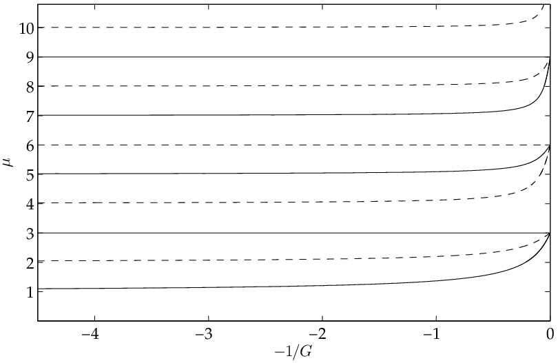
Figure 3: Solutions to (17) (even parity, dashed lines) and (18) (odd parity, solid lines) as functions of −1/G-1/G.

Allowing μ≥1\mu\geq 1 to take non-integer values, the solutions for a repulsive interaction G≥0G\geq 0 are seen on figure 3. This figure is interpreted as the angular energy spectrum (putting ν=η=0\nu=\eta=0 and neglecting the constant off-set energy) for our naïve ‘toy model’ for the system, where we neglect the coupling between ϕ\phi and ρ\rho for g>0g>0. Generally it is not the spectrum for the initial Hamiltonian, but rather some unknown toy model Hamiltonian that allows factorized wave functions. It is apparent that the factorized wave function should solve the initial problem with GG dependent on ρ\rho in the non-interacting case G=0⇔g=0G=0\Leftrightarrow g=0.

Solving eqs. (17) and (18) for the allowed values of μ\mu in the non-interacting limit yields22 2 In this notation a≡bca\equiv_{b}c means aa is congruent to cc modulo bb.

g=0:{μ=2,4,6​…≡20(even parity)μ=1,3,5​…≡21(odd parity)\displaystyle g=0:\quad\begin{cases}\mu=2,4,6\ldots&\hskip 10.00002pt\equiv_{2}0\qquad\text{(even parity)}\\ \mu=1,3,5\ldots&\hskip 10.00002pt\equiv_{2}1\qquad\text{(odd parity)}\end{cases}

Combined with eq. (16) this implies that

g=0:{f(μ,ϕ)=sin(μϕ),μ≡20(even parity)f(μ,ϕ)=cos(μϕ),μ≡21(odd parity)\displaystyle g=0:\quad\begin{cases}f(\mu,\phi)=\sin(\mu\phi)\;,\quad&\mu\equiv_{2}0\qquad\text{(even parity)}\\ f(\mu,\phi)=\cos(\mu\phi)\;,\quad&\mu\equiv_{2}1\qquad\text{(odd parity)}\end{cases}

Solving eqs. (17) and (18) for the interacting case g≠0g\neq 0 yields the following integer solutions:

g≠0:{μ=6,12,18​…≡60(even parity)μ=3,9,15​…≡63(odd parity)\displaystyle g\neq 0:\quad\begin{cases}\mu=6,12,18\ldots&\equiv_{6}0\qquad\text{(even parity)}\\ \mu=3,9,15\ldots&\equiv_{6}3\qquad\text{(odd parity)}\end{cases}

Notice that we generally have, that even (odd) parity solutions have μ\mu even (odd).

Now, let us discuss the property of the g≠0g\neq 0 solutions just obtained. Regardless of parity, they are characterized by μ≡30\mu\equiv_{3}0 and seen as the horizontal lines in figure 3. Thus they are independent of GG (and gg), so these wave functions also solve the initial problem with g>0g>0. The reason for this is, that the wave function is zero on the lines of interaction ϕ=±π6\phi=\pm\tfrac{\pi}{6}, i.e. whenever two particles meet. This is a very important observation, because it means that ⟨V⟩=0\langle V\rangle=0 for all values of gg. One may say, that these states never “feel” the interaction, and thus never need to adjust to it. For this reason, we call them the non-interacting states.

We also see that at 1/G=01/G=0 all other states become degenerate with these non-interacting states and hence demand the wave function to vanish whenever two particles meet. In fact, it does not surprise us, that only the wave functions that vanish on the lines of interaction are acceptable in the strongly interacting limit, since otherwise ⟨V⟩\langle V\rangle would diverge as G→∞G\rightarrow\infty. This has been discussed previously in the context of fermionic systems in Refs. [39, 46]

To obtain the full set of solutions for the initial problem (with G=2​g​ρG=\sqrt{2}g\rho) at 1/g=01/g=0 we note that the corresponding wave function should also be of factorized form. This observation follows since eq. (13) can only be satisfied for infinite interaction if the wave function vanishes when two particles meet. The angular and radial parts becomes independent since two particles meet on a line which is solely determined by ϕ\phi. The only wave functions that are factorized in ρ\rho and ϕ\phi coordinates in each region of figure 2 and vanish whenever two particles meet are the non-interacting solutions obtained above. Thus, if we can construct orthogonal wave functions using these non-interacting states we actually have an analytic expression for the wave functions in the strongly interacting limit [37]. We take the wave functions for the non-interacting states and multiply them with a number aia_{i} in every domain I, II and III on figure 2:

ψη(z)ψν,μ≡30(ρ,ϕ)⋅{aIin IaIIin IIaIIIin III\psi_{\eta}(z)\,\psi_{\nu,\mu\equiv_{3}0}(\rho,\phi)\cdot\begin{cases}a_{\text{I}}\quad&\text{in I}\\ a_{\text{II}}\quad&\text{in II}\\ a_{\text{III}}\quad&\text{in III}\end{cases} (19)

The subscript μ≡30\mu\equiv_{3}0 indicates that only these values are acceptable, while ν\nu and η\eta may still be any non-negative integer. Obviously, there will be the non-interacting state with the same wave function for infinite repulsion as in the g=0g=0 limit, so its wave function in the strongly interacting limit must have (aI,aII,aIII)=(1,1,1)(a_{\text{I}},a_{\text{II}},a_{\text{III}})=(1,1,1), i.e. we multiply by one in every domain. We want to create orthogonal wave functions with definite parity, and (up to some nonphysical phase factors) this can only be done by choosing the domain coefficients as (aI,aII,aIII)=(1,−2,1)(a_{\text{I}},a_{\text{II}},a_{\text{III}})=(1,-2,1) and (aI,aII,aIII)=(1,0,−1)(a_{\text{I}},a_{\text{II}},a_{\text{III}})=(1,0,-1).33 3 Which state is odd and which is even is not decided by the domain coefficients alone, but also from the symmetry/antisymmetry of the g=0g=0 wave function over the ϕ=0\phi=0 line. This concludes the construction of the wave functions for the energy and parity eigenbasis in the strongly interacting limit.

It is clear that the energy in the two interaction limits is given as 32+2​ν+μ+η\tfrac{3}{2}+2\nu+\mu+\eta with the discussed restriction μ≡30\mu\equiv_{3}0 in the strongly interacting limit. Thus, the toy model spectrum depicted on figure 3 reduces to the correct angular excitation spectrum in these limits. This suggests that the spectrum for the initial problem should look similar to the toy model spectrum, as we somehow have to connect these limits to obtain the spectrum for 0<g<∞0<g<\infty. However, bear in mind that the toy model spectrum, being a function of G=2​g​ρG=\sqrt{2}g\rho, will force us to pick a value of ρ\rho if we want to map it to a spectrum depending on gg. Later, we will do this, but first we will introduce a more sophisticated way of handling the problem for intermediate values of the interaction strength.

Refer to caption
Figure 4: The angular functions for the first six states in the μ\mu spectrum in the two limits g=0g=0 (upper row) and 1/g=01/g=0.

IV Approximated wave functions

In this section we will use the factorized wave function presented in the previous section to describe the system with 0≤g<∞0\leq g<\infty. We will calculate and discuss the energies and probability densities of the approximated wave functions.

IV.1 Assumptions

To construct our variational wave function we make two assumptions about the system: i) the first one is about the adiabatic connection of the states between g=0g=0 and 1/g=01/g=0 limits where the wave functions should have factorized form as discussed above, and ii) inspired by the discussion in the previous section we assume that it is more important to describe the angular part of the wave function, since the interaction happens on ϕ=ϕ0\phi=\phi_{0} line, so we fix the radial quantum number and find the angular part that minimizes the energy.

Suppose we have adiabatically evolved the system from the initial state |ν,μ0,η⟩\left|\nu,\mu_{0},\eta\right> at g=0g=0 to the state at 1/g=01/g=0. What would the final state be? Clearly, the center-of-mass quantum number η\eta and the parity eigenvalue would be the same, but ν\nu and μ\mu are generally not good quantum numbers for intermediate values of gg and can in principle be very different in two limits. However, having in mind the toy model with constant GG from the previous section, we assume that the state evolves smoothly into the wave function which has a spatial profile as similar as possible to the profile of the initial wave function with changes happening mostly in the angular part, i.e. we assume that the final state has ν\nu unchanged. In the same spirit we assume that μ\mu is μ0\mu_{0} rounded up to the nearest multiple of three. These assumptions were proven numerically to be true for the lowest part of the energy spectrum, as we will see later in this report. To demonstrate this adiabatic connection we show the angular functions, f⁡(μ,ϕ)f(\mu,\phi), for the first six states in the μ\mu spectrum in the g=0g=0 limit in the upper row of figure 4. In the lower row we have the first six angular functions at 1/g=01/g=0 constructed from the g=0g=0 angular functions by using the domain coefficients discussed above. The functions are labeled fμ0g​(μ,ϕ)f_{\mu_{0}}^{g}(\mu,\phi), where μ0\mu_{0} is a label to keep track of the states as there are three different states for every allowed value of μ\mu at 1/g=01/g=0, in our assumption the label is the g=0g=0 value for the angular excitation quantum number. Note that the parity eigenvalue is given by (−1)μ0(-1)^{\mu_{0}}.

As we have already noted in the previous section, the wave function for the relative motion can in general only be of the factorized form (11) when g=0g=0 or 1/g=01/g=0. Nevertheless, since we are only seeking an approximate solution to the interacting state wave functions, we assume a factorized relative wave function also for intermediate values of the interaction strength. Assuming that any state is characterized by constant ν\nu, μ0\mu_{0} and η\eta we denote this state by |ν,μ0,η⟩gap\left|\nu,\mu_{0},\eta\right>_{g}^{\text{ap}}, where we have put an superscript ‘ap’ on the state ket to indicate the approximation. We now aim to find a reasonable form for the wave function. If we consider the individual states in figure 4, we can qualitatively understand how the wave function behaves for 0<g<∞0<g<\infty. The wave function is forced to vanish for ϕ=±π6\phi=\pm\tfrac{\pi}{6}, and so we can imagine gripping these points on the g=0g=0 wave function and slowly pulling them down towards zero when gg increases. Pursuing this idea, we construct angular functions with this property that reduces to the angular functions characterized by μ0\mu_{0} in the limits, i.e.

⟨ρ,ϕ,z|ν,μ0,η⟩gap=ψη(z)Rν(μ,ρ)fμ0g(μ,ϕ)\displaystyle\left<\rho,\phi,z\,\left|\right.\!\nu,\mu_{0},\eta\right>_{g}^{\text{ap}}=\psi_{\eta}(z)R_{\nu}(\mu,\rho)f_{\mu_{0}}^{g}(\mu,\phi) (20)

where the radial part given as in eq. (11)

Rν(μ,ρ)=ALν(μ)(ρ2)e−ρ2/2ρμ.\displaystyle R_{\nu}(\mu,\rho)=A\,L_{\nu}^{(\mu)}\!\big(\rho^{2}\big)\,e^{-\rho^{2}/2}\,\rho^{\mu}\,\;. (21)

The true dependency on (ρ,ϕ)(\rho,\phi) is unknown for any gg from the interval ]0,∞[]0,\infty[, but since the above functional form is correct at the boundaries of this interval, we take it as a reasonable approximation. We assume that μ\mu is a continuous variable and a function of the interaction strength, μ=μ⁡(g)\mu=\mu(g). It looses its meaning as a quantum number for the intermediate values of gg, and we think of it as a variational parameter. For a given value of gg we will vary μ⁡(g)\mu(g) such that the energy matrix element with the approximated wave function is minimal. We again would like to stress the difference between the state labeling number μ0\mu_{0} and the variational parameter μ⁡(g)\mu(g). For the ground state (μ0=1\mu_{0}=1) the limits are μ⁡(0)=1\mu(0)=1 and μ⁡(∞)=3\mu(\infty)=3, and for the first excited state (μ0=2\mu_{0}=2), we have μ⁡(0)=2\mu(0)=2 and μ⁡(∞)=3\mu(\infty)=3. In general, a state labeled by μ0=1,2,3,…\mu_{0}=1,2,3,\dots has by definition μ⁡(0)=μ0\mu(0)=\mu_{0}, and μ⁡(∞)\mu(\infty) is μ0\mu_{0} rounded up to the nearest multiple of three. With these assumptions, it can be shown (see appendix B) that

fμ0g​(μ,ϕ)\displaystyle f_{\mu_{0}}^{g}(\mu,\phi) (22)
={sin⁡(μ⁡(π2−ϕ))in I(−1)μ0+1​sin⁡(μ⁡(π6−ϕ))+sin⁡(μ⁡(π6+ϕ))in II(−1)μ0+1​sin⁡(μ⁡(π2+ϕ))in III\displaystyle=\begin{cases}\sin\left(\mu\left(\tfrac{\pi}{2}-\phi\right)\right)&\text{in I}\\[5.0pt] (-1)^{\mu_{0}+1}\sin\left(\mu\left(\tfrac{\pi}{6}-\phi\right)\right)+\sin\left(\mu\left(\tfrac{\pi}{6}+\phi\right)\right)&\text{in II}\\[5.0pt] (-1)^{\mu_{0}+1}\sin\left(\mu\left(\tfrac{\pi}{2}+\phi\right)\right)&\text{in III}\end{cases}

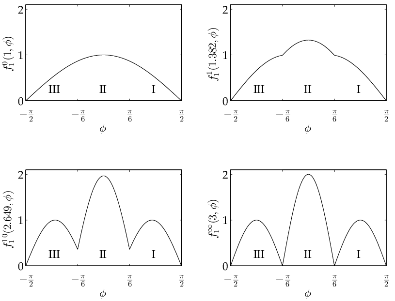
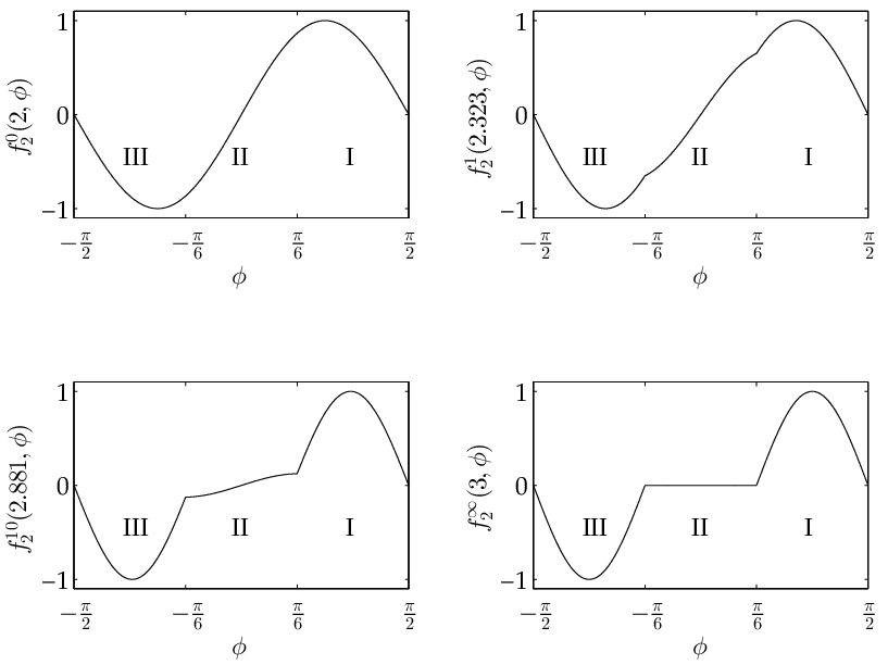
is an angular function with the right parity that reduces to the solutions in the limits g→0g\rightarrow 0 and g→∞g\rightarrow\infty that we assume are adiabatically connected. It has been found by proposing a general ansatz function with the desired parity and the property that it vanishes at ϕ=±π2\phi=\pm\tfrac{\pi}{2} as required by the Pauli principle, and at ϕ=±π6\phi=\pm\tfrac{\pi}{6} for μ=3,6,9,…\mu=3,6,9,\dots For a few values of μ\mu, this function is plotted in figure 5, where we clearly see the discussed behavior.

With the assertion of (20) as the wave function for the relative motion, the approximation for the full wave function including the center-of-mass part becomes

ψ⁡(ρ,ϕ,z)≈ψη​(z)​Rν​(μ,ρ)​fμ0g​(μ,ϕ),\displaystyle\psi(\rho,\phi,z)\approx\psi_{\eta}(z)\,R_{\nu}(\mu,\rho)\,f_{\mu_{0}}^{g}(\mu,\phi)\;, (23)
Refer to caption
Refer to caption
Figure 5: The angular function for the ground state, f1g​(μ,ϕ)f_{1}^{g}(\mu,\phi) (left side, odd parity), and the first excited state, f2g​(μ,ϕ)f_{2}^{g}(\mu,\phi) (right side, even parity), for g=0,1,10g=0,1,10 and 1/g=01/g=0. The corresponding values of μ\mu are in interval [1,3][1,3] and [2,3][2,3], respectively. It is explained in the text how μ\mu is chosen for every value of gg.

IV.2 The Hamiltonian matrix elements

The approximated interacting state wave functions (23) and the non-interacting state wave functions form a basis in which we would like to investigate the representation of the Hamiltonian. Thus we calculate the matrix elements for HH in this basis. This serves two purposes: i) we need the expectation value of a given approximated wave function to be able to variationally determine the correspondence between gg and μ\mu, and ii) we want to diagonalize the Hamiltonian in a selected subset of basis wave functions, thus getting even closer to the correct wave functions and the energy spectrum. We consider three cases for the states involved in the matrix element. Firstly, if the two states are both non-interacting, we obviously get

⟨ν′,μ0′,η′|H|ν,μ0,η⟩\displaystyle\left<\nu^{\prime},\mu_{0}^{\prime},\eta^{\prime}\vphantom{H}\right|H\left|\nu,\mu_{0},\eta\vphantom{H}\right>
=(32+2​ν+μ0+η)​δν′​ν​δμ0′​μ0​δη′​η\displaystyle=\left(\tfrac{3}{2}+2\nu+\mu_{0}+\eta\right)\delta_{\nu^{\prime}\nu}\,\delta_{\mu_{0}^{\prime}\mu_{0}}\,\delta_{\eta^{\prime}\eta} (24)

as they are both eigenstates of HH for all values of gg. Secondly, the matrix element between an interacting and a non-interacting state is zero. This is shown in Appendix C, where we also show that the matrix element between two approximated interacting states is given as

⟨ν′,μ0′,η′|H|ν,μ0,η⟩ggapap\displaystyle\mathchoice{\hphantom{{}^{{{\text{ap}}}}_{{{g}}}}\left<\nu^{\prime},\mu_{0}^{\prime},\eta^{\prime}\vphantom{H\mu_{0}^{\prime}}\right|H\left|\vphantom{H\mu_{0}^{\prime}}\nu,\mu_{0},\eta\right>^{{\kern-109.50928pt{\text{ap}}\kern 104.22594pt{\text{ap}}}}_{{\kern-106.84999pt{g}\kern 104.22594pt{g}}}}{\hphantom{{}^{{{\text{ap}}}}_{{{g}}}}\left<\nu^{\prime},\mu_{0}^{\prime},\eta^{\prime}\vphantom{H\mu_{0}^{\prime}}\right|H\left|\vphantom{H\mu_{0}^{\prime}}\nu,\mu_{0},\eta\right>^{{\kern-109.50928pt{\text{ap}}\kern 104.22594pt{\text{ap}}}}_{{\kern-106.84999pt{g}\kern 104.22594pt{g}}}}{\hphantom{{}^{{{\text{ap}}}}_{{{g}}}}\left<\nu^{\prime},\mu_{0}^{\prime},\eta^{\prime}\vphantom{H\mu_{0}^{\prime}}\right|H\left|\vphantom{H\mu_{0}^{\prime}}\nu,\mu_{0},\eta\right>^{{\kern-66.45009pt{\text{ap}}\kern 62.64453pt{\text{ap}}}}_{{\kern-64.5506pt{g}\kern 62.64453pt{g}}}}{\hphantom{{}^{{{\text{ap}}}}_{{{g}}}}\left<\nu^{\prime},\mu_{0}^{\prime},\eta^{\prime}\vphantom{H\mu_{0}^{\prime}}\right|H\left|\vphantom{H\mu_{0}^{\prime}}\nu,\mu_{0},\eta\right>^{{\kern-51.95874pt{\text{ap}}\kern 48.15318pt{\text{ap}}}}_{{\kern-50.05925pt{g}\kern 48.15318pt{g}}}} =⟨ν′,μ0′,η′|H0|ν,μ0,η⟩ggapap+⟨ν′,μ0′,η′|V|ν,μ0,η⟩ggapapwith\displaystyle=\mathchoice{\hphantom{{}^{{{\text{ap}}}}_{{{g}}}}\left<\nu^{\prime},\mu_{0}^{\prime},\eta^{\prime}\vphantom{H_{0}\mu_{0}^{\prime}}\right|H_{0}\left|\vphantom{H_{0}\mu_{0}^{\prime}}\nu,\mu_{0},\eta\right>^{{\kern-118.35927pt{\text{ap}}\kern 113.07593pt{\text{ap}}}}_{{\kern-115.69998pt{g}\kern 113.07593pt{g}}}}{\hphantom{{}^{{{\text{ap}}}}_{{{g}}}}\left<\nu^{\prime},\mu_{0}^{\prime},\eta^{\prime}\vphantom{H_{0}\mu_{0}^{\prime}}\right|H_{0}\left|\vphantom{H_{0}\mu_{0}^{\prime}}\nu,\mu_{0},\eta\right>^{{\kern-118.35927pt{\text{ap}}\kern 113.07593pt{\text{ap}}}}_{{\kern-115.69998pt{g}\kern 113.07593pt{g}}}}{\hphantom{{}^{{{\text{ap}}}}_{{{g}}}}\left<\nu^{\prime},\mu_{0}^{\prime},\eta^{\prime}\vphantom{H_{0}\mu_{0}^{\prime}}\right|H_{0}\left|\vphantom{H_{0}\mu_{0}^{\prime}}\nu,\mu_{0},\eta\right>^{{\kern-73.20009pt{\text{ap}}\kern 69.39453pt{\text{ap}}}}_{{\kern-71.3006pt{g}\kern 69.39453pt{g}}}}{\hphantom{{}^{{{\text{ap}}}}_{{{g}}}}\left<\nu^{\prime},\mu_{0}^{\prime},\eta^{\prime}\vphantom{H_{0}\mu_{0}^{\prime}}\right|H_{0}\left|\vphantom{H_{0}\mu_{0}^{\prime}}\nu,\mu_{0},\eta\right>^{{\kern-58.70874pt{\text{ap}}\kern 54.90318pt{\text{ap}}}}_{{\kern-56.80925pt{g}\kern 54.90318pt{g}}}}+\mathchoice{\hphantom{{}^{{{\text{ap}}}}_{{{g}}}}\left<\nu^{\prime},\mu_{0}^{\prime},\eta^{\prime}\vphantom{V\mu_{0}^{\prime}}\right|V\left|\vphantom{V\mu_{0}^{\prime}}\nu,\mu_{0},\eta\right>^{{\kern-107.5885pt{\text{ap}}\kern 102.30516pt{\text{ap}}}}_{{\kern-104.92921pt{g}\kern 102.30516pt{g}}}}{\hphantom{{}^{{{\text{ap}}}}_{{{g}}}}\left<\nu^{\prime},\mu_{0}^{\prime},\eta^{\prime}\vphantom{V\mu_{0}^{\prime}}\right|V\left|\vphantom{V\mu_{0}^{\prime}}\nu,\mu_{0},\eta\right>^{{\kern-107.5885pt{\text{ap}}\kern 102.30516pt{\text{ap}}}}_{{\kern-104.92921pt{g}\kern 102.30516pt{g}}}}{\hphantom{{}^{{{\text{ap}}}}_{{{g}}}}\left<\nu^{\prime},\mu_{0}^{\prime},\eta^{\prime}\vphantom{V\mu_{0}^{\prime}}\right|V\left|\vphantom{V\mu_{0}^{\prime}}\nu,\mu_{0},\eta\right>^{{\kern-64.87804pt{\text{ap}}\kern 61.07248pt{\text{ap}}}}_{{\kern-62.97855pt{g}\kern 61.07248pt{g}}}}{\hphantom{{}^{{{\text{ap}}}}_{{{g}}}}\left<\nu^{\prime},\mu_{0}^{\prime},\eta^{\prime}\vphantom{V\mu_{0}^{\prime}}\right|V\left|\vphantom{V\mu_{0}^{\prime}}\nu,\mu_{0},\eta\right>^{{\kern-50.8358pt{\text{ap}}\kern 47.03024pt{\text{ap}}}}_{{\kern-48.93631pt{g}\kern 47.03024pt{g}}}}\qquad\text{with} (25)
⟨ν′,μ0′,η′|H0|ν,μ0,η⟩ggapap\displaystyle\mathchoice{\hphantom{{}^{{{\text{ap}}}}_{{{g}}}}\left<\nu^{\prime},\mu_{0}^{\prime},\eta^{\prime}\vphantom{H_{0}\mu_{0}^{\prime}}\right|H_{0}\left|\vphantom{H_{0}\mu_{0}^{\prime}}\nu,\mu_{0},\eta\right>^{{\kern-118.35927pt{\text{ap}}\kern 113.07593pt{\text{ap}}}}_{{\kern-115.69998pt{g}\kern 113.07593pt{g}}}}{\hphantom{{}^{{{\text{ap}}}}_{{{g}}}}\left<\nu^{\prime},\mu_{0}^{\prime},\eta^{\prime}\vphantom{H_{0}\mu_{0}^{\prime}}\right|H_{0}\left|\vphantom{H_{0}\mu_{0}^{\prime}}\nu,\mu_{0},\eta\right>^{{\kern-118.35927pt{\text{ap}}\kern 113.07593pt{\text{ap}}}}_{{\kern-115.69998pt{g}\kern 113.07593pt{g}}}}{\hphantom{{}^{{{\text{ap}}}}_{{{g}}}}\left<\nu^{\prime},\mu_{0}^{\prime},\eta^{\prime}\vphantom{H_{0}\mu_{0}^{\prime}}\right|H_{0}\left|\vphantom{H_{0}\mu_{0}^{\prime}}\nu,\mu_{0},\eta\right>^{{\kern-73.20009pt{\text{ap}}\kern 69.39453pt{\text{ap}}}}_{{\kern-71.3006pt{g}\kern 69.39453pt{g}}}}{\hphantom{{}^{{{\text{ap}}}}_{{{g}}}}\left<\nu^{\prime},\mu_{0}^{\prime},\eta^{\prime}\vphantom{H_{0}\mu_{0}^{\prime}}\right|H_{0}\left|\vphantom{H_{0}\mu_{0}^{\prime}}\nu,\mu_{0},\eta\right>^{{\kern-58.70874pt{\text{ap}}\kern 54.90318pt{\text{ap}}}}_{{\kern-56.80925pt{g}\kern 54.90318pt{g}}}} =δη′​η​(32+2​ν+μ+η)​∫0∞d​ρ​ρ​Rν′​(μ′,ρ)​Rν​(μ,ρ)​∫−ππd​ϕ​fμ0′g​(μ′,ϕ)​fμ0g​(μ,ϕ)\displaystyle=\delta_{\eta^{\prime}\eta}\left(\tfrac{3}{2}+2\nu+\mu+\eta\right)\int\limits_{0}^{\infty}\mathrm{d}\rho\,\rho\,R_{\nu^{\prime}}(\mu^{\prime},\rho)R_{\nu}(\mu,\rho)\int\limits_{-\pi}^{\pi}\mathrm{d}\phi\,f_{\mu_{0}^{\prime}}^{g}(\mu^{\prime},\phi)f_{\mu_{0}}^{g}(\mu,\phi)
+δη′​η(1+(−1)μ0′+μ0)μsin(μ′π3)(2cos(μπ3)+(−1)μ0)∫0∞dρρ−1Rν′(μ′,ρ)Rν(μ,ρ),\displaystyle+\delta_{\eta^{\prime}\eta}\left(1+(-1)^{\mu_{0}^{\prime}+\mu_{0}}\right)\mu\sin\left(\mu^{\prime}\tfrac{\pi}{3}\right)\left(2\cos\left(\mu\tfrac{\pi}{3}\right)+(-1)^{\mu_{0}}\right)\int\limits_{0}^{\infty}\mathrm{d}\rho\,\rho^{-1}\,R_{\nu^{\prime}}(\mu^{\prime},\rho)R_{\nu}(\mu,\rho)\;, (26)
⟨ν′,μ0′,η′|V|ν,μ0,η⟩ggapap\displaystyle\mathchoice{\hphantom{{}^{{{\text{ap}}}}_{{{g}}}}\left<\nu^{\prime},\mu_{0}^{\prime},\eta^{\prime}\vphantom{V\mu_{0}^{\prime}}\right|V\left|\vphantom{V\mu_{0}^{\prime}}\nu,\mu_{0},\eta\right>^{{\kern-107.5885pt{\text{ap}}\kern 102.30516pt{\text{ap}}}}_{{\kern-104.92921pt{g}\kern 102.30516pt{g}}}}{\hphantom{{}^{{{\text{ap}}}}_{{{g}}}}\left<\nu^{\prime},\mu_{0}^{\prime},\eta^{\prime}\vphantom{V\mu_{0}^{\prime}}\right|V\left|\vphantom{V\mu_{0}^{\prime}}\nu,\mu_{0},\eta\right>^{{\kern-107.5885pt{\text{ap}}\kern 102.30516pt{\text{ap}}}}_{{\kern-104.92921pt{g}\kern 102.30516pt{g}}}}{\hphantom{{}^{{{\text{ap}}}}_{{{g}}}}\left<\nu^{\prime},\mu_{0}^{\prime},\eta^{\prime}\vphantom{V\mu_{0}^{\prime}}\right|V\left|\vphantom{V\mu_{0}^{\prime}}\nu,\mu_{0},\eta\right>^{{\kern-64.87804pt{\text{ap}}\kern 61.07248pt{\text{ap}}}}_{{\kern-62.97855pt{g}\kern 61.07248pt{g}}}}{\hphantom{{}^{{{\text{ap}}}}_{{{g}}}}\left<\nu^{\prime},\mu_{0}^{\prime},\eta^{\prime}\vphantom{V\mu_{0}^{\prime}}\right|V\left|\vphantom{V\mu_{0}^{\prime}}\nu,\mu_{0},\eta\right>^{{\kern-50.8358pt{\text{ap}}\kern 47.03024pt{\text{ap}}}}_{{\kern-48.93631pt{g}\kern 47.03024pt{g}}}} =δη′​η​g​2​(1+(−1)μ0′+μ0)​sin⁡(μ′​π3)​sin⁡(μ​π3)​∫0∞d​ρ​Rν′​(μ′,ρ)​Rν​(μ,ρ).\displaystyle=\delta_{\eta^{\prime}\eta}\,g\,\sqrt{2}\left(1+(-1)^{\mu_{0}^{\prime}+\mu_{0}}\right)\sin\left(\mu^{\prime}\tfrac{\pi}{3}\right)\,\sin\left(\mu\tfrac{\pi}{3}\right)\int\limits_{0}^{\infty}\mathrm{d}\rho\,R_{\nu^{\prime}}(\mu^{\prime},\rho)R_{\nu}(\mu,\rho)\;. (27)

Note that the matrix elements between two states with different center-of-mass excitation or different parity always vanishes, as it should. Also note that the states with different values of ν\nu can mix with one another.

For a given interacting state and a given value of gg, we need a criteria to choose the value of μ\mu. It seems natural to take a variational approach to this problem. For a given value of the interaction strength gg, we will consider the diagonal matrix element for that state, i.e. its expectation value, ϵ≡⟨H⟩=⟨ν,μ0,η|H|ν,μ0,η⟩ggapap\epsilon\equiv\langle H\rangle=\mathchoice{\hphantom{{}^{{{\text{ap}}}}_{{{g}}}}\left<\nu,\mu_{0},\eta\vphantom{H\mu_{0}}\right|H\left|\vphantom{H\mu_{0}}\nu,\mu_{0},\eta\right>^{{\kern-105.8143pt{\text{ap}}\kern 100.53096pt{\text{ap}}}}_{{\kern-103.15501pt{g}\kern 100.53096pt{g}}}}{\hphantom{{}^{{{\text{ap}}}}_{{{g}}}}\left<\nu,\mu_{0},\eta\vphantom{H\mu_{0}}\right|H\left|\vphantom{H\mu_{0}}\nu,\mu_{0},\eta\right>^{{\kern-105.8143pt{\text{ap}}\kern 100.53096pt{\text{ap}}}}_{{\kern-103.15501pt{g}\kern 100.53096pt{g}}}}{\hphantom{{}^{{{\text{ap}}}}_{{{g}}}}\left<\nu,\mu_{0},\eta\vphantom{H\mu_{0}}\right|H\left|\vphantom{H\mu_{0}}\nu,\mu_{0},\eta\right>^{{\kern-63.5251pt{\text{ap}}\kern 59.71954pt{\text{ap}}}}_{{\kern-61.62561pt{g}\kern 59.71954pt{g}}}}{\hphantom{{}^{{{\text{ap}}}}_{{{g}}}}\left<\nu,\mu_{0},\eta\vphantom{H\mu_{0}}\right|H\left|\vphantom{H\mu_{0}}\nu,\mu_{0},\eta\right>^{{\kern-49.03375pt{\text{ap}}\kern 45.2282pt{\text{ap}}}}_{{\kern-47.13426pt{g}\kern 45.2282pt{g}}}}, and vary μ\mu such that this expectation value is minimal. Since ϵ\epsilon is linear in gg, but a very complicated function of μ\mu, we pull gg outside the interaction term such that ⟨V⟩=g​⟨V′⟩\langle V\rangle=g\langle V^{\prime}\rangle. Notice that ⟨H0⟩\langle H_{0}\rangle and ⟨V′⟩\langle V^{\prime}\rangle are determined solely by μ\mu. If for all g∈]0,∞[g\in]0,\infty[ there is a local minimum in the trial energy ϵ⁡(μ)\epsilon(\mu) at some value μmin\mu_{\text{min}}, we can find μmin\mu_{\text{min}} for every value of gg from equation

d​ϵd​μ|μmin=dd​μ​⟨H0⟩|μmin+g​dd​μ​⟨V′⟩|μmin=0.\displaystyle\frac{\mathrm{d}\epsilon}{\mathrm{d}\mu}\!\left.\vphantom{\frac{\mathrm{d}}{\mathrm{d}\mu}}\right|_{\mu_{\text{min}}}=\left.\frac{\mathrm{d}}{\mathrm{d}\mu}\left<H_{0}\right>\right|_{\mu_{\text{min}}}+g\left.\frac{\mathrm{d}}{\mathrm{d}\mu}\left<V^{\prime}\right>\right|_{\mu_{\text{min}}}=0.

This gives us the relationship between μ\mu and gg that minimizes ϵ\epsilon:

g⁡(μ)=−dd​μ​⟨H0⟩dd​μ​⟨V′⟩.\displaystyle g(\mu)=-\,\frac{\frac{\mathrm{d}}{\mathrm{d}\mu}\left<H_{0}\right>}{\frac{\mathrm{d}}{\mathrm{d}\mu}\left<V^{\prime}\right>}\;. (28)

Using (26) and (27) it is possible to find an analytic form for this expression.

For the ground state |0,1,0⟩gap\left|0,1,0\right>_{g}^{\text{ap}} and first excited state in the η=0\eta=0 spectrum, |0,2,0⟩gap\left|0,2,0\right>_{g}^{\text{ap}}, we use eqs. (26) and (27) to calculate analytic expressions for ⟨H0⟩\langle H_{0}\rangle and ⟨V⟩\langle V\rangle, as shown in Appendix C. Then eq. (28) is used to establish the energy minimizing relation between gg and μ\mu. The analytic expression for g⁡(μ)g(\mu) is very lengthy and not very informative, so we will not quote it here. The equation gives the value of gg for a given μmin\mu_{\text{min}}, but one would rather provide a value for the interaction strength gg and find μmin\mu_{\text{min}}. This is achieved simply by numerically finding the root in g⁡(μ)−gg(\mu)~-~g. For |0,1,0⟩gap\left|0,1,0\right>_{g}^{\text{ap}} and |0,2,0⟩gap\left|0,2,0\right>_{g}^{\text{ap}} we use this method to compute a list of μ\mu’s for different values of gg. Writing μ=μ0+δ​μ\mu=\mu_{0}+\delta\mu, we show a set of δ​μ\delta\mu’s for some values of gg in Table 1, some of which were used when plotting the angular functions in figure 5. We could do this for other interacting states too, but for the sake of argument we will use δ​μ\delta\mu’s minimizing the energy of |0,1,0⟩gap\left|0,1,0\right>_{g}^{\text{ap}} for all states with μ0≡31\mu_{0}\equiv_{3}1 and the δ​μ\delta\mu’s for |0,2,0⟩gap\left|0,2,0\right>_{g}^{\text{ap}} for all states with μ0≡32\mu_{0}\equiv_{3}2. This approach yields very accurate results for the energy and the wave function, so Table 1 provide a very simple access to accurate three-body wave functions without any further calculations.

μ0≡31\mu_{0}\equiv_{3}1 μ0≡32\mu_{0}\equiv_{3}2
gg δ​μ\delta\mu δ​μ\delta\mu
00 00 00
1/41/4 0.087590.08759 0.090540.09054
1/31/3 0.118350.11835 0.119570.11957
1/21/2 0.181860.18186 0.175470.17547
11 0.381920.38192 0.322780.32278
22 0.755670.75567 0.526640.52664
10/310/3 1.099181.09918 0.675180.67518
1010 1.649391.64939 0.880540.88054
2020 1.820161.82016 0.939480.93948
100100 1.963521.96352 0.987820.98782
1000010000 1.999631.99963 0.999880.99988
∞\infty 22 11
Table 1: Energy minimizing values of δ​μ\delta\mu for |0,1,0⟩gap\left|0,1,0\right>_{g}^{\text{ap}} (second column) and |0,2,0⟩gap\left|0,2,0\right>_{g}^{\text{ap}} (third column). The numbers are used for all states with the indicated μ0\mu_{0}.
Refer to caption
Figure 6: Diagonal elements, i.e. the expectation values ϵ\epsilon, (++ and lines) and eigenvalues (∘\circ) of the Hamiltonian in a basis of 54 approximated eigenstates compared to the exact energies (⋅\cdot). We only show the lowest part of the spectrum with η=0\eta=0. We see that the deviation of the expectation values and eigenvalues from the exact energies is largest at 1/g=0.51/g=0.5 and 1/g=0.31/g=0.3.

IV.3 Diagonalization of the Hamiltonian

Using the factorized function (23) with the angular parameters, μ\mu, taken from Table 1, we are able to create an arbitrarily large basis of functions in which we can diagonalize the Hamiltonian for different values of gg. As an example, we take a basis of 54 states consisting of |ν,μ0,η⟩gap\left|\nu,\mu_{0},\eta\right>_{g}^{\text{ap}} with ν∈{0,…,5}\nu\in\{0,\dots,5\}, μ0∈{1,…,9}\mu_{0}\in\{1,\dots,9\} and since states with different center-of-mass excitation do not couple, we take η=0\eta=0 for all the states. The resulting energy spectrum is shown in figure 6, where we show the eigenvalues from the diagonalization (∘\circ) together with the diagonal elements (++) discussed in the previous subsection, versus −1/g-1/g. Since we calculated analytic expressions for ϵ⁡(μ)\epsilon(\mu) for the ground and first excited state (see appendix C), we show the spectrum for these states, including the constant energy for the second excited state, as solid lines. The figure also contains the exact energies (⋅\cdot) calculated numerically by diagonalizing the total Hamiltonian for different values of gg in a large basis of eigenstates for H0H_{0} [40]. This is a fairly large computational task, and so we are interested in seeing how well the expectation values of the approximated wave functions presented here compare to the correct energies. It is seen that the expectation values, ϵ\epsilon, for the approximated wave functions are nearly spot-on the correct energies, and that the result after diagonalization with 54 states is even better, as expected. The expectation values are a little higher than the true energies, which is consistent with the presented variational approach.

Notice that when g∼1g\sim 1 then ρ\rho is dominating the value of G=2​g​ρG=\sqrt{2}\,g\,\rho, but when gg is either very small or very large, the value of ρ\rho becomes less important and the true wave function can be very well reproduced using the presented trial wave function. Thus when g∼1g\sim 1 the factorized function (23) is further away from the true wave function, and we expect the deviation of the expectation values ϵ\epsilon to be largest in this region. However, from figure 6 we see that the largest deviation is in fact found for the two sets of data points at 1/g=0.51/g=0.5 and 1/g=0.31/g=0.3.

The introduced basis of approximated wave functions has several advantages, most notable, of course, that it reduces to the eigenbasis of the Hamiltonian in the limits of weak and strong repulsion, and hence that HH becomes ‘more and more’ diagonal as we approach these limits. But we also took great advantage of the separability of the center-of-mass term and the parity symmetry of the Hamiltonian, which significantly reduced the number of non-zero off-diagonal elements. We also observe that the factorized functions (23) describe the exact wave functions very accurately which has the consequence that these factorized functions are coupled weakly by the Hamiltonian, or in other words: an eigenvector expanded in the approximated states consists nearly solely of one state.

For the sake of completeness, we also want to compare the ‘toy model’ energy spectrum from figure 3 with the exact and the approximated energies from figure 6. However, to do the comparison, we need to relate gg and G=2​g​ρG=\sqrt{2}g\rho by choosing some value of ρ\rho, see figure 7 for the choices G=2​gG=\sqrt{2}g (dotted lines) and G=gG=g (dashed lines). We compare the low energy part of these spectra with the exact energies (⋅\cdot), the expectation values for the approximated wave functions (solid lines) and the eigenvalues found from diagonalization (∘\circ), just as in figure 6. The two fixed values of ρ\rho where chosen arbitrarily, other choices yield similar spectra, and we see no particular reason for why one choice produces a more accurate spectrum than another. Surely, we retrieve the correct energies in the interaction limits, but we also find, that the toy model is quite accurate for intermediate values of gg for these particular choices of ρ\rho. However, different choices of ρ\rho would ‘stretch’ the toy model spectrum, but not change its general form. This means that even though the very simple approach to the problem of a general interaction is not a scheme for finding the correct numerical values for the energies, we may certainly learn a lot about the shape of the spectrum and thus the behavior of the system.

Refer to caption
Figure 7: Comparison between the toy model spectrum found from the solutions to (17) and (18) with G=2​gG=\sqrt{2}g (dotted lines), G=gG=g (dashed lines), diagonal elements (solid lines) and eigenvalues (∘\circ) of the Hamiltonian as in figure 6 and the exact energies (⋅\cdot).
Refer to caption
Refer to caption
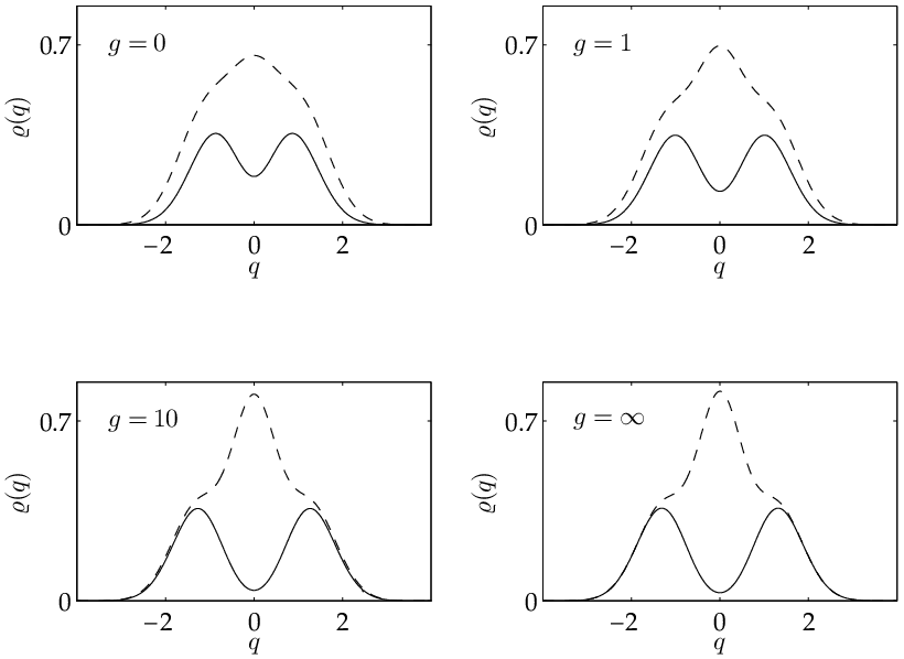
Figure 8: Probability density for particle 3 (solid) and particle 1 and 2 (dashed) for the ground state |0,1,0⟩gap\left|0,1,0\right>_{g}^{\text{ap}} (left side) and for the first excited state |0,2,0⟩gap\left|0,2,0\right>_{g}^{\text{ap}} (right side).

IV.4 Probability densities

We would like to calculate the probability density of particle ii as a function of qiq_{i} using the approximated wave functions for the ground state |0,1,0⟩gap\left|0,1,0\right>_{g}^{\text{ap}} and first excited state |0,2,0⟩gap\left|0,2,0\right>_{g}^{\text{ap}}. Using the inverse coordinate transformations, we can write the wave functions in variables (q1,q2,q3)(q_{1},q_{2},q_{3}). The desired probability density can be calculated as

ϱi(qi)=∫−∞∞dqj∫−∞∞dqk|⟨q1,q2,q3|0,μ0,0⟩gap|2,\displaystyle\varrho_{i}(q_{i})=\int\limits_{-\infty}^{\infty}\mathrm{d}q_{j}\int\limits_{-\infty}^{\infty}\mathrm{d}q_{k}\left|\left<q_{1},q_{2},q_{3}\,\left|\right.\!0,\mu_{0},0\right>_{g}^{\text{ap}}\right|^{2}\;,

where i,j,k∈{1,2,3}i,j,k\in\{1,2,3\} are all different. Since the function under the integral is piecewise-defined on domains I, …, VI, we must write the integral as a sum with one term for each domain. The domains are easily parametrized in the (q1,q2,q3)(q_{1},q_{2},q_{3}) coordinates, and for the probability density of particle 3 we get:

ϱ3​(q3)\displaystyle\varrho_{3}(q_{3}) =2​∫−∞q3d​q1​∫q1q3d​q2​|ψI|2+2​∫−∞q3d​q1​∫q3∞d​q2​|ψII|2\displaystyle=2\int\limits_{-\infty}^{q_{3}}\mathrm{d}q_{1}\int\limits_{q_{1}}^{q_{3}}\mathrm{d}q_{2}\left|\psi_{\text{I}}\right|^{2}+2\int\limits_{-\infty}^{q_{3}}\mathrm{d}q_{1}\int\limits_{q_{3}}^{\infty}\mathrm{d}q_{2}\left|\psi_{\text{II}}\right|^{2}
+2∫q3∞dq1∫q1∞dq2|ψIII|2,\displaystyle+2\int\limits_{q_{3}}^{\infty}\mathrm{d}q_{1}\int\limits_{q_{1}}^{\infty}\mathrm{d}q_{2}\left|\psi_{\text{III}}\right|^{2}\;,

where we have written ψI\psi_{\text{I}} for the wave function in domain I, and so forth, note that the contribution from the other domains, i.e. IV, V, VI is obtained from the invariance of the integrand under x↦−xx\mapsto-x. When q2≥q1q_{2}\geq q_{1} we integrate over the x≥0x\geq 0 half plane to find the probability density of particle 1:

ϱ1​(q1)\displaystyle\varrho_{1}(q_{1}) =∫q1∞d​q2​∫q2∞d​q3​|ψI|2+∫q1∞d​q2​∫q1q2d​q3​|ψII|2\displaystyle=\int\limits_{q_{1}}^{\infty}\mathrm{d}q_{2}\int\limits_{q_{2}}^{\infty}\mathrm{d}q_{3}\left|\psi_{\text{I}}\right|^{2}+\int\limits_{q_{1}}^{\infty}\mathrm{d}q_{2}\int\limits_{q_{1}}^{q_{2}}\mathrm{d}q_{3}\left|\psi_{\text{II}}\right|^{2}
+∫q1∞dq2∫−∞q1dq3|ψIII|2.\displaystyle+\int\limits_{q_{1}}^{\infty}\mathrm{d}q_{2}\int\limits_{-\infty}^{q_{1}}\mathrm{d}q_{3}\left|\psi_{\text{III}}\right|^{2}\;.

When q2≤q1q_{2}\leq q_{1} we must integrate over the x≤0x\leq 0 half plane. However, we can also use that the probability density must be invariant under reflection of the qq axis in which case we cover the situation q2≤q1q_{2}\leq q_{1} with ϱ1​(−q1)\varrho_{1}(-q_{1}). Notice that the probability density of particle 2 is equal to that of particle 1, i.e. ϱ2​(q2)=ϱ1​(q1)\varrho_{2}(q_{2})=\varrho_{1}(q_{1}), since two particles are identical. The probability densities are calculated numerically and normalized such that the integral over all densities is the number of particles. They are plotted for the ground state and for the first excited state in figure 8.

If the particles are spin-12\tfrac{1}{2} fermions, the probability densities yield some interesting magnetic behavior of the states. Say that particles 1 and 2 are indistinguishable because they are in the same spin state, for instance spin-up indicated on figure 2, opposite to the spin-down state of particle 3. For the ground state shown on the left half of figure 8 we see that when gg increases the two indistinguishable particles are “pushed” to either side of particle 3 which leads to an increasing probability to find the system in the configuration ↑↓↑\uparrow\downarrow\uparrow. Of course, particles 1 and 2 cannot be pushed completely away from particle 3 because the energy contribution from the harmonic trap potential at some point becomes too great. But as the interaction strength gg increases, particle 1 and 2 are pushed farther out to the sides of the trap. This can be interpreted as “antiferromagnetic” behavior of the few-body system, since the most energy favorable configuration is the one with alternating spin orientations along the qq-axis. For the first excited state shown on the right half of figure 8, the situation is completely different as the configuration ↑↓↑\uparrow\downarrow\uparrow becomes less probable when gg increases. In fact, from earlier we know that in the strongly interacting limit g→∞g\to\infty, the probability completely vanishes for this configuration. However, particle 3 may still be found in the middle of the harmonic trap, though the probability for doing so is very small as seen on the figure. On the other hand, the probability for finding particle 1 or 2 here is strongly favored. Particle 3 is pushed to one of the sides of the trap and the particles with the same spin orientation are located next to each other, so the first excited state exhibits “ferromagnetic” behavior. It is quite exciting to see that a small system of only three particles exhibit increasing magnetic behavior when the interaction increases. Strongly interacting particles play an important role in theories of magnetism in condensed matter physics, but the theories often consider the average behavior of many particles interacting with each other. Thus, the study of small interacting system, that are solvable in the interaction limits, like the system treated here, might lead to a better understanding of solid-state phenomena.

V Mass imbalance

Let us returning to the general three-body Hamiltonian consisting of the terms (1) and (2). Contrary to the preceding sections, the masses mim_{i} for i∈{1,2,3}i\in\{1,2,3\} are now allowed to be different. Again, we define a set of dimensionless coordinates 𝐪\bf{q} and 𝐩\bf{p}:

qi=q~iσandpi=p~i​σℏ.q_{i}=\frac{\tilde{q}_{i}}{\sigma}\quad\text{and}\quad p_{i}=\frac{\tilde{p}_{i}\,\sigma}{\hbar}\;.

where σ=ℏ/μ123​ω\sigma=\sqrt{\hbar/\mu_{123}\omega} is a length scale and μ123=m1​m2​m3/(m1+m2+m3)\mu_{123}=\sqrt{m_{1}m_{2}m_{3}/(m_{1}+m_{2}+m_{3})}. Notice that the definition of σ\sigma is now different compared to the one in Section II, since here we use a sort of reduced mass μ123\mu_{123} instead of the common mass mm. Again we choose units such that ℏ≡ω≡1\hbar\equiv\omega\equiv 1, but for pedagogical reasons we do not set μ123\mu_{123} to unity, and so contrary to before, we cannot set σ\sigma to unity. Like in Section II, we rotate the coordinates and get a new set of coordinates 𝐫=𝐉𝐪\mathbf{r}=\mathbf{J}\mathbf{q}, this time the transformation is given by

[xyz]=1μ123​[μ12−μ120μ123​m1μ12​M12μ123​m2μ12​M12−μ123μ12m1M123m2M123m3M123]​[q1q2q3],\begin{bmatrix}x\\[5.0pt] y\\[5.0pt] z\end{bmatrix}=\frac{1}{\sqrt{\mu_{123}}}\begin{bmatrix}\mu_{12}&-\mu_{12}&0\\[5.0pt] \frac{\mu_{123}m_{1}}{\mu_{12}M_{12}}&\frac{\mu_{123}m_{2}}{\mu_{12}M_{12}}&-\frac{\mu_{123}}{\mu_{12}}\\[5.0pt] \frac{m_{1}}{\sqrt{M_{123}}}&\frac{m_{2}}{\sqrt{M_{123}}}&\frac{m_{3}}{\sqrt{M_{123}}}\end{bmatrix}\begin{bmatrix}q_{1}\\[5.0pt] q_{2}\\[5.0pt] q_{3}\end{bmatrix}\;,

where M12=m1+m2M_{12}=m_{1}+m_{2}, M123=m1+m2+m3M_{123}=m_{1}+m_{2}+m_{3} and μ12=m1​m2/M12\mu_{12}=\sqrt{m_{1}m_{2}/M_{12}}. This type of transformation is chosen such that the coordinates are “rationalized”[62]. In terms of the new variables the Hamiltonian is written as:

H0\displaystyle H_{0} =12​(𝐫2−∇𝐫2)\displaystyle=\frac{1}{2}\left(\mathbf{r}^{2}-{\mbox{\boldmath$\nabla$}_{\mathbf{r}}}^{2}\right)
V\displaystyle V =[g12σμ12μ123δ(x)+g23σμ123μ12δ(μ123m1x+y)\displaystyle=\,\Bigg[\frac{g_{12}}{\sigma}\frac{\mu_{12}}{\sqrt{\mu_{123}}}\delta\!\left(x\right)+\frac{g_{23}}{\sigma}\frac{\sqrt{\mu_{123}}}{\mu_{12}}\delta\!\left(\frac{\mu_{123}}{m_{1}}x+y\right)
+g31σμ123μ12δ(−μ123m2x+y)].\displaystyle\hskip 11.38109pt+\frac{g_{31}}{\sigma}\frac{\sqrt{\mu_{123}}}{\mu_{12}}\delta\!\left(-\frac{\mu_{123}}{m_{2}}x+y\right)\Bigg]\;.

We once more notice that the full Hamiltonian is separable in terms of center-of-mass motion and the relative motion just as in the case of equal masses. For the relative motion, which happens in the x​yxy-plane we again use the (Jacobi) hyperspherical coordinates given by ρ=x2+y2\rho=\sqrt{x^{2}+y^{2}}, ρ∈[0,∞[\rho\in[0,\infty[, and tan⁡ϕ=y/x\tan\phi=y/x, ϕ∈[−π,π[\phi\in[-\pi,\pi[.

Refer to caption
Figure 9: Same as figure 2 for the mass-imbalanced case. Note that the solid lines where m=Mm=M form a 30∘30^{\circ} angle with the xx-axis. If m>Mm>M the angle decreases – shown by the dotted line and the angle goes to zero as m≫Mm\gg M. On the other hand if m<Mm<M the angle increases – shown by the dashed line and the angle goes to 45∘45^{\circ} as M≫mM\gg m. This changes the shape and size of the domains in which the function f⁡(μ,ϕ)f(\mu,\phi) lives.

Our case of interest is a system of two identical fermions and a third particle described with the following set of parameters: g12=0g_{12}=0, g23=g31=gg_{23}=g_{31}=g, m1=m2=mm_{1}=m_{2}=m and m3=Mm_{3}=M. For this case we write the Hamiltonian in terms of the hyperspherical coordinates:

H\displaystyle H =12​(z2−∂2∂z2+ρ2−1ρ​∂∂ρ−∂2∂ρ2−1ρ2​∂2∂ϕ2)\displaystyle=\frac{1}{2}\left(z^{2}-\frac{\partial^{2}}{\partial z^{2}}+\rho^{2}-\frac{1}{\rho}\frac{\partial}{\partial\rho}-\frac{\partial^{2}}{\partial\rho^{2}}-\frac{1}{\rho^{2}}\frac{\partial^{2}}{\partial\phi^{2}}\right)
+gσ​ρ2​γγ2+1∑±(δ(ϕ±θ0)+δ(ϕ±θ0−π)),\displaystyle+\frac{g}{\sigma\rho}\sqrt{\frac{2\gamma}{\gamma^{2}+1}}\sum_{\pm}\Big(\delta\big(\phi\pm\theta_{0}\big)+\delta\big(\phi\pm\theta_{0}-\pi\big)\Big)\;,

where γ≡μ123m=11+2​m/M\gamma\equiv\frac{\mu_{123}}{m}=\sqrt{\frac{1}{1+2m/M}} and θ0=arctan⁡γ\theta_{0}=\arctan\gamma is the angle between the xx-axis and the q2=q3q_{2}=q_{3} line. Notice that θ0\theta_{0} only depends on the mass ratio, thus the mass ratio determines the size of each domain in configuration space, seen on figure 9. The wave functions at the g=0g=0 and 1/g=01/g=0 limits will again be products of (10) and (11), but the conditions for finding the right angular functions f⁡(μ,ϕ)f(\mu,\phi) changes as θ0\theta_{0} is not necessarily π6\tfrac{\pi}{6}. Let us follow the same scheme as in Section III for finding the angular functions in the weakly and strongly interacting limits. First we note that the wave function for the relative motion satisfies

  1. 1.

    ψ⁡(−x,y)=−ψ⁡(x,y)\psi(-x,y)=-\psi(x,y) (Pauli principle),

  2. 2.

    ψ⁡(x,y)↦ψ⁡(−x,−y)=±ψ⁡(x,y)\psi(x,y)\mapsto\psi(-x,-y)=\pm\psi(x,y) (parity).

Next we can derive δ\delta-boundary condition similar to Eq. (14) with parameter β\beta instead of GG, β≡2​ρ​gσ​2​γγ2+1\beta\equiv\frac{2\rho g}{\sigma}\sqrt{\frac{2\gamma}{\gamma^{2}+1}}. Notice that β\beta is proportional to GG when the masses are fixed.

As before we start our analysis by treating β\beta as a constant for all hyperradii (ρ\rho) which is an effective ’toy model’ of the system. This schematic toy model employed in previous sections was introduced for equal masses in Ref. [40] and here we generalize this model to mass imbalanced 2+1 systems. As we saw in the previous section for the case of equal masses, the toy model accurately reproduces the shape of the energy spectrum of the initial Hamiltonian. After applying the conditions and solving it, one can show that for the odd parity solutions we have

μ​cos⁡(μ​π2)+β​sin⁡(μ⁡(π2−θ0))​cos⁡(μ​θ0)=0.\displaystyle\mu\cos\left(\mu\tfrac{\pi}{2}\right)+\beta\sin\left(\mu(\tfrac{\pi}{2}-\theta_{0})\right)\cos(\mu\theta_{0})=0\;. (29)

In the same way for even parity solutions parameter μ\mu satisfies the following equation

μ​sin⁡(μ​π2)+β​sin⁡(μ⁡(π2−θ0))​sin⁡(μ​θ0)=0.\displaystyle\mu\sin\left(\mu\tfrac{\pi}{2}\right)+\beta\sin\left(\mu(\tfrac{\pi}{2}-\theta_{0})\right)\sin\left(\mu\theta_{0}\right)=0\;. (30)

Notice that when m=Mm=M then γ=13\gamma=\tfrac{1}{\sqrt{3}} yielding θ0=π6\theta_{0}=\tfrac{\pi}{6}, and hence we have the same result as calculated before.

Refer to caption
Figure 10: The toy model energy spectra (solutions for μ\mu, neglecting the constant off-set energy) are shown in (a), (b) and (c) for different mass ratios. Solid lines denote odd parity solutions, and dashed lines denote even parity solutions. Notice that for β>0\beta>0 (thus g>0g>0) the ground state wave function is always odd in parity (solid). The ground state particle densities in the strongly interacting limit for the same mass ratios are shown in (d), (e) and (f). The solid line is for the single particle subsystem and the dashed line is for the 2-particle subsystem. Both are normalized to one. The angular part of the corresponding wave functions are shown for ϕ∈[−π2,π2]\phi\in[-\tfrac{\pi}{2},\tfrac{\pi}{2}] in (g), (h) and (i). Notice how the size of the domains I, II and III changes.

Fig. 10a, Fig. 10b and Fig. 10c show the energy spectrum (solutions for μ\mu to Eqs. (29) and (30)) with different mass ratios. Notice how the horizontal-line solutions for odd parity for m=Mm=M vanishes instantaneously when the mass difference is different than 11. Also the ground state for g>0g>0 remains odd in parity for any mass ratio, but the degeneracy 1/g=01/g=0 changes.

The toy model gives us knowledge of μ\mu at 1/g=01/g=0 so now we can find the ground state wave functions for strongly interacting systems. It turns out that only when M=mM=m, we can construct a ground state44 4 It is worth to note that for the excited states there might be mass ratios that allow one to construct a wave function that is non-zero in all domains. whose angular part can exist in all domains (I, II, III, IV, V and VI), whenever M<mM<m the wave function vanishes on II and V domains and whenever M>mM>m the wave function must vanish on I, III, IV and VI domains. This happens because for m≠Mm\neq M the spatial areas of I and II domains are different and the ground state should live on the domain with the largest area. This means that the number of allowed domains for angular part is reduced instantaneously for any small mass imbalance. Notice that for M<mM<m the wave function is double degenerate since there are 4 allowed domains and for M>mM>m we have a single degeneracy. We illustrate this discussion with examples for M=mM=m, M<mM<m and M>mM>m. We can find the exact wave functions at 1/g=01/g=0 in the same way as we did in section III.2. The angular part of the wave function for the ground state with M=mM=m is found to be:

f1∞​(3,ϕ)={−cos⁡(3​ϕ)in I2​cos⁡(3​ϕ)in II−cos⁡(3​ϕ)in IIIf_{1}^{\infty}(3,\phi)=\begin{cases}-\cos(3\phi)&\text{in I}\\ 2\cos(3\phi)&\text{in II}\\ -\cos(3\phi)&\text{in III}\end{cases}

where domains I, II and III are separated by the solid lines in Fig. 9. When M<mM<m, μ\mu is no longer an integer. For instance, when M=12​mM=\tfrac{1}{2}m, θ0=0.421\theta_{0}=0.421 (or 24.1∘24.1^{\circ}) and μ=2​π/[π−θ0​(rad)]≈2.731\mu=2\pi/[\pi-\theta_{0}(\text{rad})]\approx 2.731 hence the wave function is

f1∞​(μ,ϕ)={sin⁡(μ⁡(ϕ−θ0))in I0in II−sin⁡(μ⁡(ϕ+θ0))in IIIf_{1}^{\infty}(\mu,\phi)=\begin{cases}\sin(\mu(\phi-\theta_{0}))&\text{in I}\\ 0&\text{in II}\\ -\sin(\mu(\phi+\theta_{0}))&\text{in III}\end{cases}

Notice that the boundaries of domains change also: for this case the domains are separated by the dotted lines in Fig. 9. As an example of M>mM>m, we take M=2​mM=2m. In this case θ0=0.615\theta_{0}=0.615 (or 35.2∘35.2^{\circ}) and μ=π/[2​θ0​(rad)]≈2.552\mu=\pi/[2\theta_{0}(\text{rad})]\approx 2.552 and the wave function can then be constructed as

f1∞​(μ,ϕ)={0in Icos⁡(μ​ϕ)in II0in IIIf_{1}^{\infty}(\mu,\phi)=\begin{cases}0&\text{in I}\\ \cos(\mu\phi)&\text{in II}\\ 0&\text{in III}\end{cases}

The wave functions along with the corresponding densities calculated just like in section IV.4 are illustrated in Fig. 10. One might think that there would be some continuous crossover from M<mM<m to M=mM=m and then to M>mM>m but this is not the case. As shown in Fig. 10(a) the case with M=mM=m generates almost a singularity point where three states with two states of the same parity cross one another at 1/g=01/g=0. However, when MM is slightly bigger or smaller than mm, this threefold degeneracy is lifted instantly and the ground state wave function is non-zero only in certain domains.

The results presented in this section allows us to elucidate the exact behavior of the system in the strongly interaction limit. When M>mM>m we have 30∘<θ0<45∘30^{\circ}<\theta_{0}<45^{\circ} and domain II is favored for the ground state (↑↓↑\uparrow\downarrow\uparrow if we again think of spin-12\tfrac{1}{2} particles), while for M<mM<m we have 0<θ0<30∘0<\theta_{0}<30^{\circ} where domain I and III are then favored (↑↑↓\uparrow\uparrow\downarrow and ↓↑↑\downarrow\uparrow\uparrow). The special case with M=mM=m has θ0=30∘\theta_{0}=30^{\circ} and the wavefunction for the ground state is spread over all regions. It is important to notice that there is no continuous crossover going from M<mM<m to M=mM=m and then to M>mM>m for strongly interacting systems, i.e. any small infinitesimal mass imbalanced requires the wave function to vanish at a certain region and the ’accidental’ degeneracy of the spectrum at M=mM=m is immediately broken.

VI Conclusion

We studied a quantum mechanical system of three particles confined to a one-dimensional harmonic trap potential consisting of two indistinguishable fermions interacting with a third particle via a zero-range contact interaction of strength gg. We showed how the Schrödinger equation is solved in the limits of no interaction, g=0g=0, and infinitely strong repulsion, 1/g=01/g=0. Then we assumed a factorized form of the wave function for intermediate values of 0<g<∞0<g<\infty and provided a class of approximated wave functions that reduce to the analytic solutions in the limits g→0g\rightarrow 0 and g→∞g\rightarrow\infty. We produced a basis of variational wave functions for every value of gg, and we found that the resulting energy spectrum is very close to the numerically calculated energies. A diagonalization of the Hamiltonian in a basis of 54 approximated wave functions yielded even better results, as expected.

Furthermore, we calculated the probability densities of the approximated wave functions for the ground and first excited state, and discussed ferro- and antiferromagnetic behavior. In order to discuss this in the language of spin algebra, we took the three particles to be spin-12\tfrac{1}{2} particles with the two indistinguishable particles being the spin-up state, while the third particle was in the spin-down state.

Finally, we studied the case where the mass of the indistinguishable particles was allowed to differ from the mass of the third particle. This was done in a schematic ’toy model’ where the coupling is re-scaled with the hyperradius (effectively factorizing the problem). This model becomes exact in the non-interacting and strongly interacting limits. Here we find a most interesting behavior of the degeneracy of the ground state at infinite coupling strength. When the impurity is heavier than the two identical particles, we obtain a non-degenerate ground state, while in the opposite case we find a doubly degenerate ground states. The doubly degenerate ground state is also seen in the two-component bosonic system with equal masses discussed in Ref. [60]. In this sense, the equal mass case is very special with its triply degenerate ground state for strong interaction. But given that Nature provides us with numerous two-component systems of equal mass this is of course an extremely important special case at that.

This research was supported by the Danish Council for Independent Research DFF Natural Sciences and the DFF Sapere Aude program.

Appendix A Equations for μ\mu

From (15)

f⁡(μ,π2)=A​cos⁡(μ​π2)+B​sin⁡(μ​π2)=0.f\left(\mu,\tfrac{\pi}{2}\right)=A\,\cos\left(\mu\tfrac{\pi}{2}\right)+B\,\sin\left(\mu\tfrac{\pi}{2}\right)=0\;.

Considering only the states with even parity we get from (16) that

C​cos⁡(−μ​ϕ)+D​sin⁡(−μ​ϕ)=−C​cos⁡(μ​ϕ)−D​sin⁡(μ​ϕ)⇒C=0.C\,\cos(-\mu\phi)+D\,\sin(-\mu\phi)=-C\,\cos(\mu\phi)-D\,\sin(\mu\phi)\Rightarrow C=0\;.

By the continuity at ϕ=π6\phi=\tfrac{\pi}{6}

A​cos⁡(μ​π6)+B​sin⁡(μ​π6)=D​sin⁡(μ​π6),A\,\cos\left(\mu\tfrac{\pi}{6}\right)+B\,\sin\left(\mu\tfrac{\pi}{6}\right)=D\,\sin\left(\mu\tfrac{\pi}{6}\right)\;,

and finally from (14)

−μ​A​sin⁡(μ​π6)+μ​B​cos⁡(μ​π6)−μ​D​cos⁡(μ​π6)=G​D​sin⁡(μ​π6).-\mu A\,\sin\left(\mu\tfrac{\pi}{6}\right)+\mu B\,\cos\left(\mu\tfrac{\pi}{6}\right)-\mu D\,\cos\left(\mu\tfrac{\pi}{6}\right)=GD\,\sin\left(\mu\tfrac{\pi}{6}\right)\;.

Collecting these equations in a matrix equation yields

[0cos⁡(μ​π2)sin⁡(μ​π2)−sin⁡(μ​π6)cos⁡(μ​π6)sin⁡(μ​π6)−cos⁡(μ​π6)−Gμ​sin⁡(μ​π6)−sin⁡(μ​π6)cos⁡(μ​π6)]​[DAB]=[000],\begin{bmatrix}0&\cos\left(\mu\tfrac{\pi}{2}\right)&\sin\left(\mu\tfrac{\pi}{2}\right)\\[5.0pt] -\sin\left(\mu\tfrac{\pi}{6}\right)&\cos\left(\mu\tfrac{\pi}{6}\right)&\sin\left(\mu\tfrac{\pi}{6}\right)\\[5.0pt] -\cos\left(\mu\tfrac{\pi}{6}\right)-\tfrac{G}{\mu}\,\sin\left(\mu\tfrac{\pi}{6}\right)&-\sin\left(\mu\tfrac{\pi}{6}\right)&\cos\left(\mu\tfrac{\pi}{6}\right)\end{bmatrix}\begin{bmatrix}D\\[5.0pt] A\\[5.0pt] B\end{bmatrix}=\begin{bmatrix}0\\[5.0pt] 0\\[5.0pt] 0\end{bmatrix}\;,

which have a solution only if the determinant of the matrix is zero. Doing the the same calculation for odd parity, and setting the determinants of the two matrices to zero, we arrive at the equations (17) and (18).

Appendix B Approximated angular functions

We would like to find an expression for the angular part of the approximated wave function for the interacting states that have the right parity and reduces to the known solutions in the limits g→0g\rightarrow 0 and g→∞g\rightarrow\infty. First, we consider a state with odd parity (μ0\mu_{0} is odd), and fμ0g​(μ,ϕ)f_{\mu_{0}}^{g}(\mu,\phi) must therefore be symmetric around ϕ=0\phi=0. Also it must be zero when ϕ=±π2\phi=\pm\tfrac{\pi}{2}, and so we make the ansatz

fμ0g​(μ,ϕ)={sin⁡(μ⁡(π2−ϕ))in IA+B​cos⁡(μ​ϕ)in IIsin⁡(μ⁡(π2+ϕ))in IIIf_{\mu_{0}}^{g}(\mu,\phi)=\begin{cases}\sin\left(\mu\left(\tfrac{\pi}{2}-\phi\right)\right)\quad&\text{in I}\\[5.0pt] A+B\,\cos(\mu\phi)\quad&\text{in II}\\[5.0pt] \sin\left(\mu\left(\tfrac{\pi}{2}+\phi\right)\right)\quad&\text{in III}\end{cases}

Since we assume the factorized form (20) for the wave function for the relative motion, we indirectly assume that G=2​g​ρG=\sqrt{2}\,g\,\rho is independent of ρ\rho, and we apply (14) at ϕ0=π6\phi_{0}=\tfrac{\pi}{6}:

Δ⁡(∂fμ0g​(μ,ϕ)∂ϕ|π6)\displaystyle\Delta\left(\left.\frac{\partial f_{\mu_{0}}^{g}(\mu,\phi)}{\partial\phi}\right|_{\tfrac{\pi}{6}}\right) =−μ​cos⁡(μ​π3)+μ​B​sin⁡(μ​π6)\displaystyle=-\mu\,\cos\left(\mu\tfrac{\pi}{3}\right)+\mu B\,\sin\left(\mu\tfrac{\pi}{6}\right)
=G​sin⁡(μ​π3)\displaystyle=G\,\sin\left(\mu\tfrac{\pi}{3}\right)

Isolating GG from (18) and inserting in the above yields

−μ​cos⁡(μ​π3)+μ​B​sin⁡(μ​π6)=−μ​cos⁡(μ​π2)cos⁡(μ​π6),\displaystyle-\mu\,\cos\left(\mu\tfrac{\pi}{3}\right)+\mu B\,\sin\left(\mu\tfrac{\pi}{6}\right)=-\mu\,\frac{\cos\left(\mu\tfrac{\pi}{2}\right)}{\cos\left(\mu\tfrac{\pi}{6}\right)}\;,

and then we can find the constant BB as

B=1sin⁡(μ​π6)​[cos⁡(μ​π3)−cos⁡(μ​π2)cos⁡(μ​π6)]=2​sin⁡(μ​π6).B=\frac{1}{\sin\left(\mu\tfrac{\pi}{6}\right)}\left[\cos\left(\mu\tfrac{\pi}{3}\right)-\frac{\cos\left(\mu\tfrac{\pi}{2}\right)}{\cos\left(\mu\tfrac{\pi}{6}\right)}\right]=2\,\sin\left(\mu\tfrac{\pi}{6}\right)\;.

The function must be continuous at ϕ=π6\phi=\tfrac{\pi}{6}:

A+B​cos⁡(μ​π6)=sin⁡(μ​π3),A+B\,\cos\left(\mu\tfrac{\pi}{6}\right)=\sin\left(\mu\tfrac{\pi}{3}\right)\;,

and then AA is found as

A=sin⁡(μ​π3)−B​cos⁡(μ​π6)=0.A=\sin\left(\mu\tfrac{\pi}{3}\right)-B\,\cos\left(\mu\tfrac{\pi}{6}\right)=0\;.

The angular function in domain II can be written as

A+B​cos⁡(μ​ϕ)=sin⁡(μ⁡(π6−ϕ))+sin⁡(μ⁡(π6+ϕ)),A+B\,\cos(\mu\phi)=\sin\left(\mu\left(\tfrac{\pi}{6}-\phi\right)\right)+\sin\left(\mu\left(\tfrac{\pi}{6}+\phi\right)\right)\;,

and thus in total we get

fμ0g​(μ,ϕ)={sin⁡(μ⁡(π2−ϕ))in Isin⁡(μ⁡(π6−ϕ))+sin⁡(μ⁡(π6+ϕ))in IIsin⁡(μ⁡(π2+ϕ))in III\displaystyle f_{\mu_{0}}^{g}(\mu,\phi)=\begin{cases}\sin\left(\mu\left(\tfrac{\pi}{2}-\phi\right)\right)&\text{in I}\\[5.0pt] \sin\left(\mu\left(\tfrac{\pi}{6}-\phi\right)\right)+\sin\left(\mu\left(\tfrac{\pi}{6}+\phi\right)\right)&\text{in II}\\[5.0pt] \sin\left(\mu\left(\tfrac{\pi}{2}+\phi\right)\right)&\text{in III}\end{cases}

One may check that it reduces to the known solutions in the interaction limits, for instance we recover the ground state in the limits by putting μ=1\mu=1 or μ=3\mu=3.

We can do the same analysis for a state with even parity (μ0\mu_{0} is even), and we arrive at the following angular function:

fμ0g​(μ,ϕ)={sin⁡(μ⁡(π2−ϕ))in Isin⁡(μ⁡(−π6+ϕ))+sin⁡(μ⁡(π6+ϕ))in IIsin⁡(μ⁡(−π2−ϕ))in III\displaystyle f_{\mu_{0}}^{g}(\mu,\phi)=\begin{cases}\sin\left(\mu\left(\tfrac{\pi}{2}-\phi\right)\right)&\text{in I}\\[5.0pt] \sin\left(\mu\left(-\tfrac{\pi}{6}+\phi\right)\right)+\sin\left(\mu\left(\tfrac{\pi}{6}+\phi\right)\right)&\text{in II}\\[5.0pt] \sin\left(\mu\left(-\tfrac{\pi}{2}-\phi\right)\right)&\text{in III}\end{cases}

Notice that angular function for even parity is just the same as for odd parity with some signs reversed. Thus the general angular function for the interacting states can be expressed as (22) in the main text.

Appendix C The Hamiltonian matrix elements

We want to calculate the matrix elements for the Hamiltonian in the basis of approximated wave functions. As noted in the main text, we can consider three cases of a matrix element between interacting and non-interacting states, one of which (two non-interacting states) is simply (24). We now consider the case of a matrix element between an interacting and a non-interacting state. Since the Hamiltonian matrix is symmetric, we can take HH to act on the non-interacting state in which case we get

⟨ν′,μ0′,η′|H|ν,μ0,η⟩gap\displaystyle\mathchoice{\hphantom{{}^{{{\text{ap}}}}_{{{g}}}}\left<\nu^{\prime},\mu_{0}^{\prime},\eta^{\prime}\vphantom{H}\right|H\left|\vphantom{H\mu_{0}^{\prime}}\nu,\mu_{0},\eta\right>^{{\kern-101.69696pt{\text{ap}}\kern 96.41362pt}}_{{\kern-99.03767pt{g}\kern 96.41362pt}}}{\hphantom{{}^{{{\text{ap}}}}_{{{g}}}}\left<\nu^{\prime},\mu_{0}^{\prime},\eta^{\prime}\vphantom{H}\right|H\left|\vphantom{H\mu_{0}^{\prime}}\nu,\mu_{0},\eta\right>^{{\kern-101.69696pt{\text{ap}}\kern 96.41362pt}}_{{\kern-99.03767pt{g}\kern 96.41362pt}}}{\hphantom{{}^{{{\text{ap}}}}_{{{g}}}}\left<\nu^{\prime},\mu_{0}^{\prime},\eta^{\prime}\vphantom{H}\right|H\left|\vphantom{H\mu_{0}^{\prime}}\nu,\mu_{0},\eta\right>^{{\kern-61.2476pt{\text{ap}}\kern 57.44205pt}}_{{\kern-59.34811pt{g}\kern 57.44205pt}}}{\hphantom{{}^{{{\text{ap}}}}_{{{g}}}}\left<\nu^{\prime},\mu_{0}^{\prime},\eta^{\prime}\vphantom{H}\right|H\left|\vphantom{H\mu_{0}^{\prime}}\nu,\mu_{0},\eta\right>^{{\kern-47.59982pt{\text{ap}}\kern 43.79427pt}}_{{\kern-45.70033pt{g}\kern 43.79427pt}}}
=⟨ν′,μ0′,η′|H0|ν,μ0,η⟩gap\displaystyle=\mathchoice{\hphantom{{}^{{{\text{ap}}}}_{{{g}}}}\left<\nu^{\prime},\mu_{0}^{\prime},\eta^{\prime}\vphantom{H_{0}}\right|H_{0}\left|\vphantom{H_{0}\mu_{0}^{\prime}}\nu,\mu_{0},\eta\right>^{{\kern-110.54695pt{\text{ap}}\kern 105.26361pt}}_{{\kern-107.88766pt{g}\kern 105.26361pt}}}{\hphantom{{}^{{{\text{ap}}}}_{{{g}}}}\left<\nu^{\prime},\mu_{0}^{\prime},\eta^{\prime}\vphantom{H_{0}}\right|H_{0}\left|\vphantom{H_{0}\mu_{0}^{\prime}}\nu,\mu_{0},\eta\right>^{{\kern-110.54695pt{\text{ap}}\kern 105.26361pt}}_{{\kern-107.88766pt{g}\kern 105.26361pt}}}{\hphantom{{}^{{{\text{ap}}}}_{{{g}}}}\left<\nu^{\prime},\mu_{0}^{\prime},\eta^{\prime}\vphantom{H_{0}}\right|H_{0}\left|\vphantom{H_{0}\mu_{0}^{\prime}}\nu,\mu_{0},\eta\right>^{{\kern-67.9976pt{\text{ap}}\kern 64.19205pt}}_{{\kern-66.09811pt{g}\kern 64.19205pt}}}{\hphantom{{}^{{{\text{ap}}}}_{{{g}}}}\left<\nu^{\prime},\mu_{0}^{\prime},\eta^{\prime}\vphantom{H_{0}}\right|H_{0}\left|\vphantom{H_{0}\mu_{0}^{\prime}}\nu,\mu_{0},\eta\right>^{{\kern-54.34982pt{\text{ap}}\kern 50.54427pt}}_{{\kern-52.45033pt{g}\kern 50.54427pt}}}
=(32+2ν+μ0+η)⟨ν′,μ0′,η′|ν,μ0,η⟩gap\displaystyle=\left(\tfrac{3}{2}+2\nu+\mu_{0}+\eta\right)\,\mathchoice{\hphantom{{}^{{{\text{ap}}}}_{{{g}}}}\left<\nu^{\prime},\mu_{0}^{\prime},\eta^{\prime}\,\right|\left.\!\vphantom{\mu_{0}^{\prime}}\nu,\mu_{0},\eta\right>^{{\kern-80.33167pt{\text{ap}}\kern 75.04832pt}}_{{\kern-77.67238pt{g}\kern 75.04832pt}}}{\hphantom{{}^{{{\text{ap}}}}_{{{g}}}}\left<\nu^{\prime},\mu_{0}^{\prime},\eta^{\prime}\,\right|\left.\!\vphantom{\mu_{0}^{\prime}}\nu,\mu_{0},\eta\right>^{{\kern-80.33167pt{\text{ap}}\kern 75.04832pt}}_{{\kern-77.67238pt{g}\kern 75.04832pt}}}{\hphantom{{}^{{{\text{ap}}}}_{{{g}}}}\left<\nu^{\prime},\mu_{0}^{\prime},\eta^{\prime}\,\right|\left.\!\vphantom{\mu_{0}^{\prime}}\nu,\mu_{0},\eta\right>^{{\kern-48.18394pt{\text{ap}}\kern 44.37839pt}}_{{\kern-46.28445pt{g}\kern 44.37839pt}}}{\hphantom{{}^{{{\text{ap}}}}_{{{g}}}}\left<\nu^{\prime},\mu_{0}^{\prime},\eta^{\prime}\,\right|\left.\!\vphantom{\mu_{0}^{\prime}}\nu,\mu_{0},\eta\right>^{{\kern-38.60193pt{\text{ap}}\kern 34.79637pt}}_{{\kern-36.70244pt{g}\kern 34.79637pt}}}
=(32+2​ν+μ0+η)​δη′​η​∫0∞d​ρ​ρ​Rν′​(μ′,ρ)​Rν​(μ,ρ)​∫−ππd​ϕ​fμ0′g​(μ′,ϕ)​fμ0g​(μ,ϕ),\displaystyle=\left(\tfrac{3}{2}+2\nu+\mu_{0}+\eta\right)\,\delta_{\eta^{\prime}\eta}\,\int\limits_{0}^{\infty}\mathrm{d}\rho\,\rho\,R_{\nu^{\prime}}(\mu^{\prime},\rho)R_{\nu}(\mu,\rho)\int\limits_{-\pi}^{\pi}\mathrm{d}\phi\,f_{\mu_{0}^{\prime}}^{g}(\mu^{\prime},\phi)f_{\mu_{0}}^{g}(\mu,\phi)\;,

With the non-interacting angular function fμ0g​(μ,ϕ)=cos⁡(μ​ϕ)f_{\mu_{0}}^{g}(\mu,\phi)=\cos(\mu\phi) or fμ0g​(μ,ϕ)=sin⁡(μ​ϕ)f_{\mu_{0}}^{g}(\mu,\phi)=\sin(\mu\phi) with μ≡30\mu\equiv_{3}0 and fμ0′g​(μ′,ϕ)f_{\mu_{0}^{\prime}}^{g}(\mu^{\prime},\phi) given by (22), one may verify that

∫−ππd​ϕ​fμ0′g​(μ′,ϕ)​fμ0g​(μ,ϕ)=0.\displaystyle\int\limits_{-\pi}^{\pi}\mathrm{d}\phi\,f_{\mu_{0}^{\prime}}^{g}(\mu^{\prime},\phi)f_{\mu_{0}}^{g}(\mu,\phi)=0\;.

We now turn to the matrix element between two interacting states. We calculate the H0H_{0} term and VV term separately, starting with the former using (8). If the double derivative of fμ0g​(μ,ϕ)f_{\mu_{0}}^{g}(\mu,\phi) with respect to ϕ\phi was defined for every ϕ∈[−π,π[\phi\in[-\pi,\pi[, this would be straightforward. However, this is not the case since it is not continuously differentiable in ϕ=±π6\phi=\pm\tfrac{\pi}{6} and ϕ=±5​π6\phi=\pm\tfrac{5\pi}{6} when g≠0g\neq 0, so we isolate this part of the matrix element and treat it carefully.

⟨ν′,μ0′,η′|H0|ν,μ0,η⟩ggapap\displaystyle\mathchoice{\hphantom{{}^{{{\text{ap}}}}_{{{g}}}}\left<\nu^{\prime},\mu_{0}^{\prime},\eta^{\prime}\vphantom{H_{0}}\right|H_{0}\left|\vphantom{H_{0}\mu_{0}^{\prime}}\nu,\mu_{0},\eta\right>^{{\kern-110.54695pt{\text{ap}}\kern 105.26361pt{\text{ap}}}}_{{\kern-107.88766pt{g}\kern 105.26361pt{g}}}}{\hphantom{{}^{{{\text{ap}}}}_{{{g}}}}\left<\nu^{\prime},\mu_{0}^{\prime},\eta^{\prime}\vphantom{H_{0}}\right|H_{0}\left|\vphantom{H_{0}\mu_{0}^{\prime}}\nu,\mu_{0},\eta\right>^{{\kern-110.54695pt{\text{ap}}\kern 105.26361pt{\text{ap}}}}_{{\kern-107.88766pt{g}\kern 105.26361pt{g}}}}{\hphantom{{}^{{{\text{ap}}}}_{{{g}}}}\left<\nu^{\prime},\mu_{0}^{\prime},\eta^{\prime}\vphantom{H_{0}}\right|H_{0}\left|\vphantom{H_{0}\mu_{0}^{\prime}}\nu,\mu_{0},\eta\right>^{{\kern-67.9976pt{\text{ap}}\kern 64.19205pt{\text{ap}}}}_{{\kern-66.09811pt{g}\kern 64.19205pt{g}}}}{\hphantom{{}^{{{\text{ap}}}}_{{{g}}}}\left<\nu^{\prime},\mu_{0}^{\prime},\eta^{\prime}\vphantom{H_{0}}\right|H_{0}\left|\vphantom{H_{0}\mu_{0}^{\prime}}\nu,\mu_{0},\eta\right>^{{\kern-54.34982pt{\text{ap}}\kern 50.54427pt{\text{ap}}}}_{{\kern-52.45033pt{g}\kern 50.54427pt{g}}}}
=∫−∞∞d​z​∫0∞d​ρ​ρ​∫−ππd​ϕ​ψη′​(z)​Rν′​(μ′,ρ)​fμ0′g​(μ′,ϕ)​12​(z2−∂2∂z2+ρ2−1ρ​∂∂ρ−∂2∂ρ2−1ρ2​∂2∂ϕ2)​ψη​(z)​Rν​(μ,ρ)​fμ0g​(μ,ϕ)\displaystyle=\int\limits_{-\infty}^{\infty}\mathrm{d}z\int\limits_{0}^{\infty}\mathrm{d}\rho\,\rho\int\limits_{-\pi}^{\pi}\mathrm{d}\phi\,\psi_{\eta^{\prime}}(z)R_{\nu^{\prime}}(\mu^{\prime},\rho)f_{\mu_{0}^{\prime}}^{g}(\mu^{\prime},\phi)\frac{1}{2}\left(z^{2}-\frac{\partial^{2}}{\partial z^{2}}+\rho^{2}-\frac{1}{\rho}\frac{\partial}{\partial\rho}-\frac{\partial^{2}}{\partial\rho^{2}}-\frac{1}{\rho^{2}}\frac{\partial^{2}}{\partial\phi^{2}}\right)\psi_{\eta}(z)R_{\nu}(\mu,\rho)f_{\mu_{0}}^{g}(\mu,\phi)
=∫−∞∞d​z​∫0∞d​ρ​ρ​∫−ππd​ϕ​ψη′​(z)​Rν′​(μ′,ρ)​fμ0′g​(μ′,ϕ)​12​(z2−∂2∂z2+ρ2−1ρ​∂∂ρ−∂2∂ρ2+μ2ρ2)​ψη​(z)​Rν​(μ,ρ)​fμ0g​(μ,ϕ)\displaystyle=\int\limits_{-\infty}^{\infty}\mathrm{d}z\int\limits_{0}^{\infty}\mathrm{d}\rho\,\rho\int\limits_{-\pi}^{\pi}\mathrm{d}\phi\,\psi_{\eta^{\prime}}(z)R_{\nu^{\prime}}(\mu^{\prime},\rho)f_{\mu_{0}^{\prime}}^{g}(\mu^{\prime},\phi)\frac{1}{2}\left(z^{2}-\frac{\partial^{2}}{\partial z^{2}}+\rho^{2}-\frac{1}{\rho}\frac{\partial}{\partial\rho}-\frac{\partial^{2}}{\partial\rho^{2}}+\frac{\mu^{2}}{\rho^{2}}\right)\psi_{\eta}(z)R_{\nu}(\mu,\rho)f_{\mu_{0}}^{g}(\mu,\phi)
=−μ22​δη′,η​∫0∞d​ρ​ρ−1​Rν′​(μ′,ρ)​Rν​(μ,ρ)​∫−ππd​ϕ​fμ0′g​(μ′,ϕ)​fμ0g​(μ,ϕ)\displaystyle\hphantom{=}-\frac{\mu^{2}}{2}\delta_{\eta^{\prime},\eta}\int\limits_{0}^{\infty}\mathrm{d}\rho\,\rho^{-1}R_{\nu^{\prime}}(\mu^{\prime},\rho)R_{\nu}(\mu,\rho)\int\limits_{-\pi}^{\pi}\mathrm{d}\phi\,f_{\mu_{0}^{\prime}}^{g}(\mu^{\prime},\phi)f_{\mu_{0}}^{g}(\mu,\phi)
=−12​δη′,η​∫0∞d​ρ​ρ−1​Rν′​(μ′,ρ)​Rν​(μ,ρ)​∫−ππd​ϕ​fμ0′g​(μ′,ϕ)​∂2∂ϕ2​fμ0g​(μ,ϕ)\displaystyle\hphantom{=}-\frac{1}{2}\delta_{\eta^{\prime},\eta}\int\limits_{0}^{\infty}\mathrm{d}\rho\,\rho^{-1}R_{\nu^{\prime}}(\mu^{\prime},\rho)R_{\nu}(\mu,\rho)\int\limits_{-\pi}^{\pi}\mathrm{d}\phi\,f_{\mu_{0}^{\prime}}^{g}(\mu^{\prime},\phi)\frac{\partial^{2}}{\partial\phi^{2}}f_{\mu_{0}}^{g}(\mu,\phi)

We now treat this last integral over ϕ\phi. Since the integrand is not always defined, we must divide the integral into pieces and take the limit as we integrate over the problematic points and over the intervals between them.

∫−ππd​ϕ​fμ0′g​(μ′,ϕ)​∂2∂ϕ2​fμ0g​(μ,ϕ)=limε→0(∫−π6−ε−π6+εd​ϕ​fμ0′g​(μ′,ϕ)​∂2∂ϕ2​fμ0g​(μ,ϕ)+CLOSE\displaystyle\int\limits_{-\pi}^{\pi}\mathrm{d}\phi\,f_{\mu_{0}^{\prime}}^{g}(\mu^{\prime},\phi)\frac{\partial^{2}}{\partial\phi^{2}}\,f_{\mu_{0}}^{g}(\mu,\phi)=\lim\limits_{\varepsilon\rightarrow 0}\left(\int\limits_{-\frac{\pi}{6}-\varepsilon}^{-\frac{\pi}{6}+\varepsilon}\mathrm{d}\phi\,f_{\mu_{0}^{\prime}}^{g}(\mu^{\prime},\phi)\frac{\partial^{2}}{\partial\phi^{2}}\,f_{\mu_{0}}^{g}(\mu,\phi)\right.+
OPEN∫−π6+επ6−εd​ϕ​fμ0′g​(μ′,ϕ)​∂2∂ϕ2​fμ0g​(μ,ϕ)+…+∫−5​π6+ε−π6−εd​ϕ​fμ0′g​(μ′,ϕ)​∂2∂ϕ2​fμ0g​(μ,ϕ)).\displaystyle\left.\int\limits_{-\frac{\pi}{6}+\varepsilon}^{\frac{\pi}{6}-\varepsilon}\mathrm{d}\phi\,f_{\mu_{0}^{\prime}}^{g}(\mu^{\prime},\phi)\frac{\partial^{2}}{\partial\phi^{2}}\,f_{\mu_{0}}^{g}(\mu,\phi)+\ldots+\int\limits_{-\frac{5\pi}{6}+\varepsilon}^{-\frac{\pi}{6}-\varepsilon}\mathrm{d}\phi\,f_{\mu_{0}^{\prime}}^{g}(\mu^{\prime},\phi)\frac{\partial^{2}}{\partial\phi^{2}}\,f_{\mu_{0}}^{g}(\mu,\phi)\right)\;.

Consider a ϕ0∈{±π6,±5​π6}\phi_{0}\in\big\{\pm\tfrac{\pi}{6},\pm\tfrac{5\pi}{6}\big\} and the integral over this point. Integrals of that type will in the limit ε→0\varepsilon\rightarrow 0 be evaluated as

limε→0∫ϕ0−εϕ0+εd​ϕ​fμ0′g​(μ′,ϕ)​∂2∂ϕ2​fμ0g​(μ,ϕ)\displaystyle\lim\limits_{\varepsilon\rightarrow 0}\int\limits_{\phi_{0}-\varepsilon}^{\phi_{0}+\varepsilon}\mathrm{d}\phi\,f_{\mu_{0}^{\prime}}^{g}(\mu^{\prime},\phi)\frac{\partial^{2}}{\partial\phi^{2}}\,f_{\mu_{0}}^{g}(\mu,\phi) =fμ0′g​(μ′,ϕ0)​limε→0(∂fμ0g∂ϕ|ϕ0+ε−∂fμ0g∂ϕ|ϕ0−ε)\displaystyle=f_{\mu_{0}^{\prime}}^{g}(\mu^{\prime},\phi_{0})\,\lim\limits_{\varepsilon\rightarrow 0}\left(\left.\frac{\partial f_{\mu_{0}}^{g}}{\partial\phi}\right|_{\phi_{0}+\varepsilon}-\left.\frac{\partial f_{\mu_{0}}^{g}}{\partial\phi}\right|_{\phi_{0}-\varepsilon}\right)
=fμ0′g​(μ′,ϕ0)​Δ​(∂fμ0g∂ϕ|ϕ0).\displaystyle=f_{\mu_{0}^{\prime}}^{g}(\mu^{\prime},\phi_{0})\,\Delta\left(\left.\frac{\partial f_{\mu_{0}}^{g}}{\partial\phi}\right|_{\phi_{0}}\right)\;.

It follows from the antisymmetry fμ0g​(μ,−x)=−fμ0g​(μ,x)f_{\mu_{0}}^{g}(\mu,-x)=-f_{\mu_{0}}^{g}(\mu,x) that we get the same contribution from the x>0x>0 and x<0x<0 half planes, and so we only need to compute it for ϕ0=±π6\phi_{0}=\pm\tfrac{\pi}{6}. If we plug in the angular function (22), it is easy to show that

fμ0′g​(μ′,π6)​Δ​(∂fμ0g∂ϕ|π6)+fμ0′g​(μ′,−π6)​Δ​(∂fμ0g∂ϕ|−π6)=−(1+(−1)μ0′+μ0)​μ​sin⁡(μ′​π3)​(2​cos⁡(μ​π3)+(−1)μ0)\displaystyle f_{\mu_{0}^{\prime}}^{g}(\mu^{\prime},\tfrac{\pi}{6})\,\Delta\left(\left.\frac{\partial f_{\mu_{0}}^{g}}{\partial\phi}\right|_{\tfrac{\pi}{6}}\right)+f_{\mu_{0}^{\prime}}^{g}(\mu^{\prime},-\tfrac{\pi}{6})\,\Delta\left(\left.\frac{\partial f_{\mu_{0}}^{g}}{\partial\phi}\right|_{-\tfrac{\pi}{6}}\right)=-\left(1+(-1)^{\mu_{0}^{\prime}+\mu_{0}}\right)\mu\sin\left(\mu^{\prime}\tfrac{\pi}{3}\right)\left(2\cos\left(\mu\tfrac{\pi}{3}\right)+(-1)^{\mu_{0}}\right)

On the intervals between the points where the double derivative is undefined, we have a well-defined second derivative ∂2∂ϕ2​fμ0g​(μ,ϕ)=−μ2​fμ0g​(μ,ϕ)\frac{\partial^{2}}{\partial\phi^{2}}f_{\mu_{0}}^{g}(\mu,\phi)=-\mu^{2}f_{\mu_{0}}^{g}(\mu,\phi). The sum of integrals over these intervals have the limit

limε→0(∫−π6+επ6−εdϕfμ0′g(μ′,ϕ)∂2∂ϕ2fμ0g(μ,ϕ)+…+∫5​π6+ε−π6−εdϕfμ0′g(μ′,ϕ)∂2∂ϕ2fμ0g(μ,ϕ))=−μ2∫−ππdϕfμ0′g(μ′,ϕ)fμ0g(μ,ϕ).\displaystyle\lim\limits_{\varepsilon\rightarrow 0}\left(\int\limits_{-\tfrac{\pi}{6}+\varepsilon}^{\tfrac{\pi}{6}-\varepsilon}\mathrm{d}\phi\,f_{\mu_{0}^{\prime}}^{g}(\mu^{\prime},\phi)\frac{\partial^{2}}{\partial\phi^{2}}\,f_{\mu_{0}}^{g}(\mu,\phi)+\ldots+\int\limits_{\tfrac{5\pi}{6}+\varepsilon}^{-\tfrac{\pi}{6}-\varepsilon}\mathrm{d}\phi\,f_{\mu_{0}^{\prime}}^{g}(\mu^{\prime},\phi)\frac{\partial^{2}}{\partial\phi^{2}}\,f_{\mu_{0}}^{g}(\mu,\phi)\right)=-\mu^{2}\int\limits_{-\pi}^{\pi}\mathrm{d}\phi\,f_{\mu_{0}^{\prime}}^{g}(\mu^{\prime},\phi)f_{\mu_{0}}^{g}(\mu,\phi)\;.

Thus

∫−ππd​ϕ​fμ0′g​(μ′,ϕ)​∂2∂ϕ2​fμ0g​(μ,ϕ)\displaystyle\int\limits_{-\pi}^{\pi}\mathrm{d}\phi\,f_{\mu_{0}^{\prime}}^{g}(\mu^{\prime},\phi)\frac{\partial^{2}}{\partial\phi^{2}}f_{\mu_{0}}^{g}(\mu,\phi)
=−2​(1+(−1)μ0′+μ0)​μ​sin⁡(μ′​π3)​(2​cos⁡(μ​π3)+(−1)μ0)−μ2​∫−ππd​ϕ​fμ0′g​(μ′,ϕ)​fμ0g​(μ,ϕ).\displaystyle=-2\left(1+(-1)^{\mu_{0}^{\prime}+\mu_{0}}\right)\mu\sin\left(\mu^{\prime}\tfrac{\pi}{3}\right)\left(2\cos\left(\mu\tfrac{\pi}{3}\right)+(-1)^{\mu_{0}}\right)-\mu^{2}\int\limits_{-\pi}^{\pi}\mathrm{d}\phi\,f_{\mu_{0}^{\prime}}^{g}(\mu^{\prime},\phi)f_{\mu_{0}}^{g}(\mu,\phi)\;.

Using that

12​(z2−∂2∂z2+ρ2−1ρ​∂∂ρ−∂2∂ρ2+μ2ρ2)​ψη​(z)​Rν​(μ,ρ)​fμ0g​(μ,ϕ)=(32+2​ν+μ+η)​ψη​(z)​Rν​(μ,ρ)​fμ0g​(μ,ϕ)\displaystyle\frac{1}{2}\left(z^{2}-\frac{\partial^{2}}{\partial z^{2}}+\rho^{2}-\frac{1}{\rho}\frac{\partial}{\partial\rho}-\frac{\partial^{2}}{\partial\rho^{2}}+\frac{\mu^{2}}{\rho^{2}}\right)\psi_{\eta}(z)R_{\nu}(\mu,\rho)f_{\mu_{0}}^{g}(\mu,\phi)=\left(\tfrac{3}{2}+2\nu+\mu+\eta\right)\psi_{\eta}(z)R_{\nu}(\mu,\rho)f_{\mu_{0}}^{g}(\mu,\phi)

and the orthogonality of ψη​(z)\psi_{\eta}(z)’s, it is now straightforward to rewrite the matrix element on the form (26).

For the interaction term, we use (9) and evaluate (22) at the specified points, yielding

⟨ν′,μ0′,η′|V|ν,μ0,η⟩ggapap\displaystyle\mathchoice{\hphantom{{}^{{{\text{ap}}}}_{{{g}}}}\left<\nu^{\prime},\mu_{0}^{\prime},\eta^{\prime}\vphantom{V\mu_{0}^{\prime}}\right|V\left|\vphantom{V\mu_{0}^{\prime}}\nu,\mu_{0},\eta\right>^{{\kern-107.5885pt{\text{ap}}\kern 102.30516pt{\text{ap}}}}_{{\kern-104.92921pt{g}\kern 102.30516pt{g}}}}{\hphantom{{}^{{{\text{ap}}}}_{{{g}}}}\left<\nu^{\prime},\mu_{0}^{\prime},\eta^{\prime}\vphantom{V\mu_{0}^{\prime}}\right|V\left|\vphantom{V\mu_{0}^{\prime}}\nu,\mu_{0},\eta\right>^{{\kern-107.5885pt{\text{ap}}\kern 102.30516pt{\text{ap}}}}_{{\kern-104.92921pt{g}\kern 102.30516pt{g}}}}{\hphantom{{}^{{{\text{ap}}}}_{{{g}}}}\left<\nu^{\prime},\mu_{0}^{\prime},\eta^{\prime}\vphantom{V\mu_{0}^{\prime}}\right|V\left|\vphantom{V\mu_{0}^{\prime}}\nu,\mu_{0},\eta\right>^{{\kern-64.87804pt{\text{ap}}\kern 61.07248pt{\text{ap}}}}_{{\kern-62.97855pt{g}\kern 61.07248pt{g}}}}{\hphantom{{}^{{{\text{ap}}}}_{{{g}}}}\left<\nu^{\prime},\mu_{0}^{\prime},\eta^{\prime}\vphantom{V\mu_{0}^{\prime}}\right|V\left|\vphantom{V\mu_{0}^{\prime}}\nu,\mu_{0},\eta\right>^{{\kern-50.8358pt{\text{ap}}\kern 47.03024pt{\text{ap}}}}_{{\kern-48.93631pt{g}\kern 47.03024pt{g}}}}
=∫−∞∞d​z​∫0∞d​ρ​ρ​∫−ππd​ϕ​ψη′​(z)​Rν′​(μ′,ρ)​fμ0′g​(μ′,ϕ)\displaystyle=\int\limits_{-\infty}^{\infty}\mathrm{d}z\int\limits_{0}^{\infty}\mathrm{d}\rho\,\rho\int\limits_{-\pi}^{\pi}\mathrm{d}\phi\,\psi_{\eta^{\prime}}(z)R_{\nu^{\prime}}(\mu^{\prime},\rho)f_{\mu_{0}^{\prime}}^{g}(\mu^{\prime},\phi)
=×g2​ρ​[δ⁡(ϕ−π6)+δ⁡(ϕ+5​π6)+δ⁡(ϕ+π6)+δ⁡(ϕ−5​π6)]​ψη​(z)​Rν​(μ,ρ)​fμ0g​(μ,ϕ)\displaystyle\hphantom{=}\times\frac{g}{\sqrt{2}\,\rho}\Big[\delta\!\left(\phi-\tfrac{\pi}{6}\right)+\delta\!\left(\phi+\tfrac{5\pi}{6}\right)+\delta\!\left(\phi+\tfrac{\pi}{6}\right)+\delta\!\left(\phi-\tfrac{5\pi}{6}\right)\Big]\psi_{\eta}(z)R_{\nu}(\mu,\rho)f_{\mu_{0}}^{g}(\mu,\phi)
=g2​δη′,η​∫0∞d​ρ​Rν′​(μ′,ρ)​Rν​(μ,ρ)​(2​sin⁡(μ′​π3)​sin⁡(μ​π3)+2​(−1)μ0′+μ0​sin⁡(μ′​π3)​sin⁡(μ​π3))\displaystyle=\frac{g}{\sqrt{2}}\delta_{\eta^{\prime},\eta}\int\limits_{0}^{\infty}\mathrm{d}\rho\,R_{\nu^{\prime}}(\mu^{\prime},\rho)R_{\nu}(\mu,\rho)\left(2\sin(\mu^{\prime}\tfrac{\pi}{3})\sin(\mu\tfrac{\pi}{3})+2(-1)^{\mu_{0}^{\prime}+\mu_{0}}\sin(\mu^{\prime}\tfrac{\pi}{3})\sin(\mu\tfrac{\pi}{3})\right)

from which (27) follows immediately.

The matrix elements for H0H_{0} and VV for the ground state |0,1,0⟩gap\left|0,1,0\right>_{g}^{\text{ap}} and first excited state |0,2,0⟩gap\left|0,2,0\right>_{g}^{\text{ap}} are found to be

⟨0,1,0​|H0|​0,1,0⟩ggapap=32+μ+Γ⁡(μ)Γ⁡(μ+1)​μ2​sin⁡(π3​μ)​(2​cos⁡(π3​μ)−1)2​π3​μ−π3​μ​cos⁡(π3​μ)+sin⁡(π3​μ)−sin⁡(2​π3​μ)\displaystyle\mathchoice{\hphantom{{}^{{{\text{ap}}}}_{{{g}}}}\left<0,1,0\vphantom{H_{0}}\left|H_{0}\right|\vphantom{H_{0}}0,1,0\right>^{{\kern-91.07289pt{\text{ap}}\kern 85.78955pt{\text{ap}}}}_{{\kern-88.4136pt{g}\kern 85.78955pt{g}}}}{\hphantom{{}^{{{\text{ap}}}}_{{{g}}}}\left<0,1,0\vphantom{H_{0}}\left|H_{0}\right|\vphantom{H_{0}}0,1,0\right>^{{\kern-91.07289pt{\text{ap}}\kern 85.78955pt{\text{ap}}}}_{{\kern-88.4136pt{g}\kern 85.78955pt{g}}}}{\hphantom{{}^{{{\text{ap}}}}_{{{g}}}}\left<0,1,0\vphantom{H_{0}}\left|H_{0}\right|\vphantom{H_{0}}0,1,0\right>^{{\kern-54.45811pt{\text{ap}}\kern 50.65256pt{\text{ap}}}}_{{\kern-52.55862pt{g}\kern 50.65256pt{g}}}}{\hphantom{{}^{{{\text{ap}}}}_{{{g}}}}\left<0,1,0\vphantom{H_{0}}\left|H_{0}\right|\vphantom{H_{0}}0,1,0\right>^{{\kern-41.91452pt{\text{ap}}\kern 38.10896pt{\text{ap}}}}_{{\kern-40.01503pt{g}\kern 38.10896pt{g}}}}=\frac{3}{2}+\mu+\frac{\Gamma(\mu)}{\Gamma(\mu+1)}\frac{\mu^{2}\sin\left(\frac{\pi}{3}\mu\right)\left(2\cos\left(\frac{\pi}{3}\mu\right)-1\right)}{\tfrac{2\pi}{3}\mu-\tfrac{\pi}{3}\mu\cos\left(\frac{\pi}{3}\mu\right)+\sin\left(\frac{\pi}{3}\mu\right)-\sin\left(\frac{2\pi}{3}\mu\right)}
⟨0,1,0​|V|​0,1,0⟩ggapap=g​Γ⁡(μ+12)Γ⁡(μ+1)​2​μ​sin2⁡(π3​μ)2​π3​μ−π3​μ​cos⁡(π3​μ)+sin⁡(π3​μ)−sin⁡(2​π3​μ)\displaystyle\mathchoice{\hphantom{{}^{{{\text{ap}}}}_{{{g}}}}\left<0,1,0\vphantom{V}\left|V\right|\vphantom{V}0,1,0\right>^{{\kern-80.30212pt{\text{ap}}\kern 75.01878pt{\text{ap}}}}_{{\kern-77.64284pt{g}\kern 75.01878pt{g}}}}{\hphantom{{}^{{{\text{ap}}}}_{{{g}}}}\left<0,1,0\vphantom{V}\left|V\right|\vphantom{V}0,1,0\right>^{{\kern-80.30212pt{\text{ap}}\kern 75.01878pt{\text{ap}}}}_{{\kern-77.64284pt{g}\kern 75.01878pt{g}}}}{\hphantom{{}^{{{\text{ap}}}}_{{{g}}}}\left<0,1,0\vphantom{V}\left|V\right|\vphantom{V}0,1,0\right>^{{\kern-46.13606pt{\text{ap}}\kern 42.3305pt{\text{ap}}}}_{{\kern-44.23657pt{g}\kern 42.3305pt{g}}}}{\hphantom{{}^{{{\text{ap}}}}_{{{g}}}}\left<0,1,0\vphantom{V}\left|V\right|\vphantom{V}0,1,0\right>^{{\kern-34.04158pt{\text{ap}}\kern 30.23602pt{\text{ap}}}}_{{\kern-32.14209pt{g}\kern 30.23602pt{g}}}}=g\,\frac{\Gamma\big(\mu+\tfrac{1}{2}\big)}{\Gamma(\mu+1)}\frac{\sqrt{2}\mu\sin^{2}\left(\frac{\pi}{3}\mu\right)}{\tfrac{2\pi}{3}\mu-\tfrac{\pi}{3}\mu\cos\left(\frac{\pi}{3}\mu\right)+\sin\left(\frac{\pi}{3}\mu\right)-\sin\left(\frac{2\pi}{3}\mu\right)}
⟨0,2,0​|H0|​0,2,0⟩ggapap=32+μ+Γ⁡(μ)Γ⁡(μ+1)​μ2​sin⁡(π3​μ)​(2​cos⁡(π3​μ)+1)2​π3​μ+π3​μ​cos⁡(π3​μ)−sin⁡(π3​μ)−sin⁡(2​π3​μ)\displaystyle\mathchoice{\hphantom{{}^{{{\text{ap}}}}_{{{g}}}}\left<0,2,0\vphantom{H_{0}}\left|H_{0}\right|\vphantom{H_{0}}0,2,0\right>^{{\kern-91.07289pt{\text{ap}}\kern 85.78955pt{\text{ap}}}}_{{\kern-88.4136pt{g}\kern 85.78955pt{g}}}}{\hphantom{{}^{{{\text{ap}}}}_{{{g}}}}\left<0,2,0\vphantom{H_{0}}\left|H_{0}\right|\vphantom{H_{0}}0,2,0\right>^{{\kern-91.07289pt{\text{ap}}\kern 85.78955pt{\text{ap}}}}_{{\kern-88.4136pt{g}\kern 85.78955pt{g}}}}{\hphantom{{}^{{{\text{ap}}}}_{{{g}}}}\left<0,2,0\vphantom{H_{0}}\left|H_{0}\right|\vphantom{H_{0}}0,2,0\right>^{{\kern-54.45811pt{\text{ap}}\kern 50.65256pt{\text{ap}}}}_{{\kern-52.55862pt{g}\kern 50.65256pt{g}}}}{\hphantom{{}^{{{\text{ap}}}}_{{{g}}}}\left<0,2,0\vphantom{H_{0}}\left|H_{0}\right|\vphantom{H_{0}}0,2,0\right>^{{\kern-41.91452pt{\text{ap}}\kern 38.10896pt{\text{ap}}}}_{{\kern-40.01503pt{g}\kern 38.10896pt{g}}}}=\frac{3}{2}+\mu+\frac{\Gamma(\mu)}{\Gamma(\mu+1)}\frac{\mu^{2}\sin\left(\frac{\pi}{3}\mu\right)\left(2\cos\left(\frac{\pi}{3}\mu\right)+1\right)}{\tfrac{2\pi}{3}\mu+\tfrac{\pi}{3}\mu\cos\left(\frac{\pi}{3}\mu\right)-\sin\left(\frac{\pi}{3}\mu\right)-\sin\left(\frac{2\pi}{3}\mu\right)}
⟨0,2,0​|V|​0,2,0⟩ggapap=g​Γ⁡(μ+12)Γ⁡(μ+1)​2​μ​sin2⁡(π3​μ)2​π3​μ+π3​μ​cos⁡(π3​μ)−sin⁡(π3​μ)−sin⁡(2​π3​μ).\displaystyle\mathchoice{\hphantom{{}^{{{\text{ap}}}}_{{{g}}}}\left<0,2,0\vphantom{V}\left|V\right|\vphantom{V}0,2,0\right>^{{\kern-80.30212pt{\text{ap}}\kern 75.01878pt{\text{ap}}}}_{{\kern-77.64284pt{g}\kern 75.01878pt{g}}}}{\hphantom{{}^{{{\text{ap}}}}_{{{g}}}}\left<0,2,0\vphantom{V}\left|V\right|\vphantom{V}0,2,0\right>^{{\kern-80.30212pt{\text{ap}}\kern 75.01878pt{\text{ap}}}}_{{\kern-77.64284pt{g}\kern 75.01878pt{g}}}}{\hphantom{{}^{{{\text{ap}}}}_{{{g}}}}\left<0,2,0\vphantom{V}\left|V\right|\vphantom{V}0,2,0\right>^{{\kern-46.13606pt{\text{ap}}\kern 42.3305pt{\text{ap}}}}_{{\kern-44.23657pt{g}\kern 42.3305pt{g}}}}{\hphantom{{}^{{{\text{ap}}}}_{{{g}}}}\left<0,2,0\vphantom{V}\left|V\right|\vphantom{V}0,2,0\right>^{{\kern-34.04158pt{\text{ap}}\kern 30.23602pt{\text{ap}}}}_{{\kern-32.14209pt{g}\kern 30.23602pt{g}}}}=g\,\frac{\Gamma\big(\mu+\tfrac{1}{2}\big)}{\Gamma(\mu+1)}\frac{\sqrt{2}\mu\sin^{2}\left(\frac{\pi}{3}\mu\right)}{\tfrac{2\pi}{3}\mu+\tfrac{\pi}{3}\mu\cos\left(\frac{\pi}{3}\mu\right)-\sin\left(\frac{\pi}{3}\mu\right)-\sin\left(\frac{2\pi}{3}\mu\right)}\;.

References

  • [1] F. Serwane et al., Science 332, 6027 (2011).
  • [2] G. Zürn et al., Phys. Rev. Lett. 108, 075303 (2012).
  • [3] A. Wenz et al., Science 342, 457 (2013).
  • [4] G. Zürn et al., Phys. Rev. Lett. 111, 175302 (2013).
  • [5] S. Will, T. Best, S. Braun, U. Schneider, and I. Bloch, Phys. Rev. Lett. 106, 115305 (2011).
  • [6] F. Nogrette et al., Phys. Rev. X 4, 021034 (2014).
  • [7] H. Labuhn et al., Phys. Rev. A 90, 023415 (2014).
  • [8] S. Will et al., Phys. Rev. Lett. 113, 147205 (2014).
  • [9] I. Bloch, J. Dalibard, and W. Zwerger, Rev. Mod. Phys. 80, 885 (2008).
  • [10] C. Chin, R. Grimm, P. S. Julienne, and E. Tiesinga, Rev. Mod. Phys. 82, 1225 (2010).
  • [11] B. Sutherland: Beautiful Models (World Scientific, Singapore, 2004).
  • [12] M. A. Cazalilla et al., Rev. Mod. Phys. Rev. Mod. Phys. 83, 1405 (2011).
  • [13] B. Paredes et al., Nature 429, 277 (2004).
  • [14] T. Kinoshita, T. Wenger, and D. S. Weiss, Science 305, 1125 (2004).
  • [15] T. Kinoshita, T. Wenger, and D. S. Weiss, Phys. Rev. Lett. 95, 190406 (2005).
  • [16] L. W. Tonks, Phys. Rev. 50, 955 (1936).
  • [17] M. D. Girardeau, J. Math. Phys. 1, 516 (1960).
  • [18] M. Olshanii, Phys. Rev. Lett. 81, 938 (1998).
  • [19] G. E. Astrakharchik, J. Boronat, J. Casulleras, and S. Giorgini, Phys. Rev. Lett. 95, 190407 (2005).
  • [20] E. Haller et al., Science 325, 1224 (2009).
  • [21] S. Zöllner, H.-D. Meyer, and P Schmelcher, Phys. Rev. A 74, 063611 (2006); Phys. Rev. A 75, 043608 (2007); Phys. Rev. Lett. 100, 040401 (2008).
  • [22] F. Deuretzbacher, K. Bongs, K. Sengstock, and D. Pfannkuche, Phys. Rev. A 75, 013614 (2007).
  • [23] E. Tempfli, S. Zöllner, and P. Schmelcher, New J. Phys. 11, 073015 (2009).
  • [24] M. D. Girardeau, Phys. Rev. A 83, 011601(R) (2011).
  • [25] I. Brouzos and P. Schmelcher, Phys. Rev. Lett. 108, 045301 (2012).
  • [26] I. Brouzos and A. Förster, Phys. Rev. A 89, 053632 (2014).
  • [27] B. Wilson, A. Förster, C. C. N. Kuhn, I. Roditi, and D. Rubeni, Phys. Lett. A 378, 1065 (2014).
  • [28] N. T. Zinner et al., Europhys. Lett. 107, 60003 (2014).
  • [29] L. Guan, S. Chen, Y. Wang, and Z.-Q. Ma, Phys. Rev. Lett. 102, 160402 (2009).
  • [30] C. N. Yang, Chin. Phys. Lett. 26, 120504 (2009).
  • [31] M. D. Girardeau, Phys. Rev. A 82, 011607(R) (2010).
  • [32] L. Guan and S. Chen, Phys. Rev. Lett. 105, 175301 (2010).
  • [33] D. Rubeni, A. Förster, and I. Roditi, Phys. Rev. A 86, 043619 (2012).
  • [34] G. E. Astrakharchik and I. Brouzos, Phys. Rev. A 88, 021602(R) (2013).
  • [35] I. Brouzos and P. Schmelcher, Phys. Rev. A 87, 023605 (2013).
  • [36] P. O. Bugnion and G. J. Conduit, Phys. Rev. A 87, 060502(R) (2013).
  • [37] S. E. Gharashi and D. Blume, Phys. Rev. Lett. 111, 045302 (2013).
  • [38] T. Sowiński, T. Grass, O. Dutta, and M. Lewenstein, Phys. Rev. A 88, 033607 (2013).
  • [39] A. G. Volosniev et al., Nature Commun. 5, 5300 (2014).
  • [40] E. J. Lindgren et al., New J. Phys. 16, 063003 (2014).
  • [41] S. E. Gharashi, X. Y. Yin, and D. Blume, Phys. Rev. A 89, 023603 (2014).
  • [42] F. Deuretzbacher, D. Becker, J. Bjerlin, S. M. Reimann, and L. Santos, Phys. Rev. A 90, 013611 (2014).
  • [43] A. G. Volosniev et al., arXiv:1408.3414 (2014).
  • [44] X. Cui and T.-L. Ho, Phys. Rev. A 89, 023611 (2014).
  • [45] T. Sowiński, M. Gajda, and K. Rza̧żewski, Europhys. Lett. 109, 26005 (2015).
  • [46] J. Levinsen, P. Massignan, G. M. Bruun, and M. M. Parish, arXiv:1408.7096 (2014).
  • [47] M. D. Girardeau and M. Olshanii, Phys. Rev. A 70, 023608 (2004).
  • [48] M. D. Girardeau and A. Minguzzi, Phys. Rev. Lett. 99, 230402 (2007).
  • [49] S. Zöllner, H.-D. Meyer, and P Schmelcher, Phys. Rev. A 78, 013629 (2008);
  • [50] F. Deuretzbacher et al., Phys. Rev. Lett. 100, 160405 (2008).
  • [51] B. Fang, P. Vignolo, M. Gattobigio, C. Miniatura, and A. Minguzzi, Phys. Rev. A 84, 023626 (2011).
  • [52] N. L. Harshman, Phys. Rev. A 86, 052122 (2012).
  • [53] M. A. Garcia-March and Th. Busch, Phys. Rev. A 87, 063633 (2013).
  • [54] M. A. Garcia-March et al., Phys. Rev. A 88, 063604 (2013).
  • [55] N. L. Harshman, Phys. Rev. A 89, 033633 (2014).
  • [56] S. Campbell, M. A. Garcia-March, T. Fogarty, and Th. Busch, Phys. Rev. A 90, 013617 (2014).
  • [57] M. A. Garcia-March et al., New J. Phys. 16, 103004 (2014).
  • [58] P. D’Amico and M. Rontani, J. Phys. B 47, 065303 (2014); arXiv:1404.7762 (2014).
  • [59] N. P. Mehta, Phys. Rev. A 89, 052706 (2014).
  • [60] A. S. Dehkharghani et al., arXiv:1409.4224 (2014).
  • [61] M. A. Garcia-March et al., Phys. Rev. A 90, 063605 (2014).
  • [62] J. B. McGuire, J. Math. Phys. 5, 622 (1964).