Spectral density of the Dirac operator in two-flavour QCD
Abstract:
We compute the spectral density of the (Hermitean) Dirac operator in Quantum Chromodynamics with two light degenerate quarks near the origin. We use CLS/ALPHA lattices generated with two flavours of -improved Wilson fermions corresponding to pseudoscalar meson masses down to MeV, and with spacings in the range – fm. Thanks to the coverage of parameter space, we can extrapolate our data to the chiral and continuum limits with confidence. The results show that the spectral density at the origin is non-zero because the low modes of the Dirac operator do condense as expected in the Banks–Casher mechanism. Within errors, the spectral density turns out to be a constant function up to eigenvalues of MeV. Its value agrees with the one extracted from the Gell–Mann–Oakes–Renner relation.
1 Introduction
There is overwhelming evidence that the chiral symmetry group of Quantum Chromodynamics (QCD) with a small number of light flavours breaks spontaneously to . This progress became possible over the last decade thanks to the impressive speed-up of the numerical simulations of lattice QCD with light dynamical fermions [1, 2, 3, 4, 5], for a recent compilation of results see [6]. By now it is standard practice to assume this fact, and extrapolate phenomenologically interesting observables in the quark mass by applying the predictions of chiral perturbation theory (ChPT) [7, 8].
The distinctive signature of spontaneous symmetry breaking in QCD is the set of relations among pion masses and matrix elements which are expected to hold in the chiral limit [7]. Pions interact only if they carry momentum, and their matrix elements near the chiral limit can be expressed as known functions of two low-energy constants (LECs), the decay constant and the chiral condensate . The simplest of these relations is the Gell-Mann-Oakes-Renner (GMOR) one, which equals the slope of the pion mass squared with respect to the quark mass to . On the one hand lattice simulations became so powerful that we are having now the tools to verify some of these relations with confidence. On the other hand very little is known about the dynamical mechanism which breaks chiral symmetry. Maybe the spectrum of the Dirac operator is the simplest quantity to look at for an insight. Indeed many years ago Banks and Casher suggested that chiral symmetry breaks if the low modes of the Dirac operator at the origin do condense and vice-versa [9]. Remarkably we now know that the spectral density [9, 10, 11] is a renormalisable quantity to which a universal meaning can be assigned [12].
The present paper is the second of two devoted to the computation of the spectral density of the Dirac operator in QCD with two flavours near the origin11 1 Preliminary results of this work were presented in Refs. [13, 14].. This is achieved by extrapolating the numerical results obtained with -improved Wilson fermions at several lattice spacings to the universal continuum limit. In the first paper the focus was on the physics results [15], while here we report the full set of results, the technical and the numerical details of the computation. After fixing the notation and giving the parameters of the lattices simulated in the second and third sections, the fourth and the fifth ones are devoted to two different numerical analyses of the data. Results and conclusions are given in the last section.
2 Spectral density of the Dirac operator
In a space-time box of volume with periodic boundary conditions the spectral density of the Euclidean massless Dirac operator is defined as
| (1) |
where , , are its (purely imaginary) eigenvalues ordered with their magnitude in ascending order. As usual the bracket denotes the QCD expectation value and the quark mass. The spectral density is a renormalisable observable [12, 16]. Once the free parameters in the action (coupling constant and quark masses) have been renormalized, no renormalisation ambiguity is left in . The Banks–Casher relation [9]
| (2) |
links the spectral density to the chiral condensate
| (3) |
where is the quark doublet. It can be read in either directions. If chiral symmetry is spontaneously broken by a non-zero value of the condensate, the density of the quark modes in infinite volume does not vanish at the origin. Conversely a non-zero density implies that the symmetry is broken.
The mode number of the Dirac operator
| (4) |
corresponds also to the average number of eigenmodes of the massive Hermitean operator with eigenvalues . It is a renormalisation-group invariant quantity as it stands. Its (normalized) discrete derivative
| (5) |
carries the same information as , but this effective spectral density is a more convenient quantity to consider in practice on the lattice.
2.1 Mode number on the lattice
We discretize two-flavour QCD with the Wilson plaquette action for the gauge field, and O-improved Wilson action for the doublet of mass-degenerate quarks [17, 18], see appendix A for more details. The mode number22 2 We use the same notation for lattice and continuum quantities, since any ambiguity is resolved from the context. As usual the continuum limit value of a renormalised lattice quantity, identified with the subscript , is the one to be identified with its continuum counterpart. is defined as the average number of eigenmodes of the massive Hermitean O-improved Wilson-Dirac operator with eigenvalues . In the continuum limit this definition converges to the universal one [12]
| (6) |
provided is defined as in Eq. (21), and as
| (7) |
The counter-term proportional to ensures that at finite lattice spacing is an O-improved quantity. This improvement coefficient has been computed in Ref. [12], and its values for the inverse couplings considered in this paper are given in Table 3.
For Wilson fermions chiral symmetry is violated at finite lattice spacing. As a consequence the fine details of the spectrum of the Wilson–Dirac operator near the threshold is not protected from large lattice effects [16, 19, 20]. While this region may be of interest for studying the peculiar details of those fermions, it is easier to extract universal information about the continuum theory far away from it. In this respect the effective spectral density in Eq. (5) is a good quantity to consider on the lattice to extract the value of the chiral condensate33 3 Once the renormalisability of the spectral density is proven, a generic finite integral of can be used to measure the condensate, see Ref. [21] for a different choice. .
3 Numerical setup
The CLS community44 4 https://wiki-zeuthen.desy.de/CLS/CLS. and the ALPHA Collaboration have generated the gauge configurations of the two-flavour QCD with the -improved Wilson action by using the MP-HMC (lattices A5, B6, G8, N6 and O7) and the DD-HMC (all other lattices) algorithms as implemented in Refs. [22, 23]. The primary observables that we have computed are the two-point functions of bilinear operators in Eq. (20), and the mode number . The former were already computed by the ALPHA Collaboration, see Appendix B and Refs. [24, 25] for more details.
| id | MDU | [MeV] | [MeV] | [MeV] | [fm] | ||||
|---|---|---|---|---|---|---|---|---|---|
| A3 | 0.0749(8) | ||||||||
| A4 | |||||||||
| A5 | |||||||||
| B6 | |||||||||
| E5 | 0.0652(6) | ||||||||
| F6 | |||||||||
| F7 | |||||||||
| G8 | |||||||||
| N5 | 0.0483(4) | ||||||||
| N6 | |||||||||
| O7 |
3.1 Computation of the mode number
The stochastic computation of the mode number has been carried out as in Ref. [12]. A numerical approximation of the orthogonal projector to the subspace spanned by the eigenmodes of with eigenvalues is computed as
| (8) |
where . The function is an approximation to the step function by a minmax polynomial of degree in the range , see Ref. [12] for more details. This choice, together with the value of given, guarantees a systematic error well below our statistical errors. The mode number is then computed as
| (9) |
where we have added to the theory a set of pseudo-fermion fields with Gaussian action. In the course of a numerical simulation, one such field ( for each gauge-field configuration is generated randomly, and the mode number is estimated in the usual way by averaging the observable over the generated ensemble of fields. The mode number is an extensive quantity, and at fixed and for a given statistics, the relative statistical error of the calculated mode number is therefore expected to decrease like .
3.2 Ensembles generated
The details of the lattices are listed in Tables 1 and 2. All of them have a size of , and the spatial dimensions are always large enough so that . The three values of the coupling constant correspond to lattice spacings of fm respectively, which have been fixed from by supplementing the theory with a quenched “strange” quark [24]. The pion masses range from MeV to MeV. To explicitly check for finite-size effects in the mode number we have generated an additional set of lattices (D5) with the same spacing and quark mass as E5, but with a smaller lattice volume .
| id | ||||||
| A3 | 7 | 2.96 | 47.36 | 40 | ||
| A4 | 5 | 2.96 | 53.28 | |||
| A5 | 1 | 5 | 4.00 | 3 | 36.00 | |
| B6 | 1 | 6 | 2.00 | 24.00 | ||
| E5 | 9 | 5.92 | 6 | 35.52 | 55 | |
| F6 | 8 | 2.96 | 29.60 | |||
| F7 | 7 | 2.96 | 26.64 | |||
| G8 | 1 | 8 | 2.00 | 24–48 | ||
| N5 | 30 | 3.52 | 11 | 28.16 | 100 | |
| N6 | 1 | 10 | 4.00 | 128 | ||
| O7 | 1 | 15 | 4.00 | 76 |
The autocorrelation times of the two-point functions and of the mode number are reported in Table 2. For the lattice E5 we have computed for three values of corresponding to and MeV, and no significative difference was observed. We thus space the measurements to give time to the mode number to decorrelate, while we bin properly the (cheaper) measurements of the two-point functions. To measure , the number of configurations to be processed is chosen so that the statistical error of the effective spectral density receives roughly equally-sized contributions from the scale and the mode number. To ensure a proper Monte Carlo sampling, a minimum of 50 configurations is processed in any case.
The value of of the Markov chain, defined as in Ref. [24], is taken from [27]. It gets significantly longer towards finer lattice spacings. For the ensembles where , we estimate the contributions of the tails in the autocorrelation functions of the observables as described in Ref. [28]. When needed, we take them into account to have a more conservative error estimate.
4 A first look into the numerical results
We have computed the mode number for nine values55 5 If not explicitly stated, the scheme- and scale-dependent quantities such as , , and are renormalized in the scheme at GeV. of in the range – MeV with a statistical accuracy of a few percent on all lattices listed in Table 1. Four larger values of in the range – MeV have been also analysed for the ensemble E5. The results are collected in Tables 5–7 of the Appendix D.


In Figure 1 we show as a function of for the lattice O7, corresponding to the smallest reference quark mass (see below) at the smallest lattice spacing. On all other lattices an analogous qualitative behaviour is observed. The mode number is a nearly linear function in up to approximatively – MeV. A clear departure from linearity is observed for MeV on the lattice E5. At the percent precision, however, the data show statistically significant deviations from the linear behavior already below MeV. To guide the eye, a quadratic fit in is shown in Figure 1, and the values of the coefficients are given in the caption. The bulk of is given by the linear term, while the constant and the quadratic term represent corrections in the fitted range. The nearly linear behaviour of the mode number is manifest on the right plot of Figure 1, where its discrete derivative, defined as in Eq. (5) for each couple of consecutive values of , is shown as a function of . Since it is not affected by threshold effects, the effective spectral density is the primary observable we focus on in the next sections.


4.1 Continuum-limit extrapolation
In general for we observe quite a flat behaviour in
toward finer lattice spacings and light quark
masses, similar to the one shown in Figure 1. Because
the action and
the mode number are -improved, the Symanzik effective theory analysis
predicts that discretization errors start
at . In order to remove them, at every lattice spacing
we match three quark mass values (, , MeV)
by interpolating linearly in (see next section for more details).
The values of show mild discretization effects at light
and , while they differ up to per linear dimension
among the three lattice spacings toward larger . Within the
statistical errors all data sets are compatible with a linear dependence
in , and we thus independently extrapolate each triplet of points
to the continuum limit accordingly. We show six of those extrapolations
in Figure 2, considering the lightest and the heaviest reference
quark masses for
the lightest, an intermediate, and the heaviest cutoff .
The difference between the values of
at the finest lattice spacing and the continuum-extrapolated
ones is within the statistical errors for light and , and
it remains within few standard deviations toward larger values of
and . This fact makes us confident that the extrapolation removes
the cutoff effects within the errors quoted.
The results
for at MeV in the continuum limit are shown as a function
of in the left plot of Figure 3.
A similar -dependence is observed at the two other
reference masses.


It is worth noting that no assumption on the presence of spontaneous symmetry breaking was needed so far. These results, however, point to the fact that the spectral density of the Dirac operator in two-flavour QCD is (almost) constant in near the origin at small quark masses. This is consistent with the expectation from the Banks–Casher relation in presence of spontaneous symmetry breaking. In this case next-to-leading (NLO) ChPT indeed predicts
| (10) |
i.e. an almost flat function in (small) at (small) finite quark masses, see Appendix C for unexplained notation. At fixed quark mass the -dependence of in Eq. (10) is parameter-free once the pion mass and decay constant are measured.
4.2 Chiral limit
The extrapolation to the chiral limit requires an assumption on how the effective spectral density behaves when . In this respect it is interesting to note that the NLO function in Eq. (10) goes linearly in near the chiral limit since there are no chiral logarithms at fixed , see Appendix C. A fit of the data to Eq. (10) shows that the data are compatible with that NLO formula. A prediction of NLO ChPT in the two-flavour theory is that in the chiral limit also at non-zero , since all NLO corrections in Eq. (10) vanish [29]. To check for this property we extrapolate with Eq. (11), which is a generalization of Eq. (10) see below, and we obtain the results shown in the right plot of Figure 3 with a . Within errors the -dependence is clearly compatible with a constant up to MeV. Moreover the difference between the values of in the chiral limit and those at MeV is of the order of the statistical error, i.e. the extrapolation is very mild. A fit to a constant of the data gives MeV.
As in any numerical computation, the chiral limit inevitably requires an extrapolation of the results with a pre-defined functional form. The distinctive feature of spontaneous symmetry breaking, however, is that the behaviour of near the origin is predicted by ChPT, and its extrapolated value has to agree with the one of . We have thus complemented our computations with those for , and , and extrapolated the above mentioned ratio to the chiral limit as prescribed by ChPT, see Appendix B and Ref. [15]. We obtain MeV, where the first error is statistical and the second is systematic, in excellent agreement with the value quoted above. These results show that the spectral density at the origin has a non-zero value in the chiral limit. In the rest of this paper we assume this conclusion, and we apply standard field theory arguments to remove with confidence the (small) contributions in the raw data due to the discretization effects, the finite quark mass and finite .
5 Detailed discussion of numerical results
We have analysed the numerical results for the effective spectral density following two different fitting strategies. In the first one, the main results of which are reported in the previous section, we have extrapolated the results at fixed kinematics to the continuum limit independently. The results of this analysis call for an alternative strategy to extract the chiral condensate which uses ChPT from the starting point, i.e. based on fitting the data in all three directions at the same time. This procedure reduces the number of fit parameters, allows us to include all generated data in the fit, and avoids the need for an interpolation in the quark mass. It is important to stress that also in this case ChPT is used to remove only (small) higher order corrections in the spectral density. The details of these fits are reported in the next two sub-sections.
5.1 Continuum limit fit
In the first strategy outlined in Section 4 we start by interpolating the data in the quark mass at fixed and . We choose three reference values (, , MeV) which are within the range of simulated quark masses at all values, and they are as close as possible to the values at the finest lattice spacing. Most of the data sets look perfectly linear in in the vicinity of the interpolation points, with small deviations only for simultaneous coarse lattices, light ’s and towards heavy quark masses (see Figure 4). In all cases, however, the systematic error associated with the linear interpolation is negligible with respect to the statistical one. The interpolation and all following fits are performed using the jackknife technique to take into account the correlation of the data.
At fixed , each data set is well fitted by a linear function in , see Figure 2, a fact which supports the assumption of being in the Symanzik asymptotic regime within the errors quoted66 6 A detailed analysis of discretization effects in the spectral density is beyond the scope of this paper. For completeness we report the results of these fits in Appendix D for the interested readers.. Once extrapolated to the continuum limit, we fit the effective spectral density with the functional form
| (11) |
which rests on NLO ChPT, but it is capable of accounting for effects. The latter are expected to be the dominant higher order effects in ChPT in this range of parameters. Within the given accuracy, is consistent with a plateau behaviour in the range MeV, see right plot of Figure 3. By fitting to a constant in this range, we obtain MeV. If we include also a term in the fit and consider the entire range MeV we find MeV, which differs from the previous result by roughly one standard deviation. At the level of our statistical errors of , the spectral density of the Dirac operator in the continuum and chiral limits is a constant function up to MeV.
5.2 Combined fit


In this section we present an alternative strategy to extract the chiral condensate, based on fitting the data in all three directions at the same time. Compared to the first strategy, the shortcomings are that we cannot disentangle different corrections as clearly and ChPT is used from the very beginning. We remark, however, that also in this case ChPT is used only to remove higher order corrections, while the bulk of the chiral condensate is still given through the Banks–Casher relation. The statistical analysis is based on a double-elimination jackknife fit to take into account all errors and correlations (no fit of fitted quantities is needed). We start with the fit form
| (12) |
where , and we constrain the fit-parameters as suggested by NLO chiral and Symanzik effective theories. As already verified in the first strategy, the discretization effects obey an -dependence in the range of parameters simulated. We thus constrain our fit parameters to obey 77 7 Note that this expression includes also the functional form of discretization effects predicted at NLO in the GSM regime of ChPT [30], see Appendices C and E.
| (13) |
The NLO ChPT predicts that and should both be constant. Allowing for the time being an arbitrary -dependence in the parameter , we arrive at the fit function
| (14) | |||||
The fit of the data is shown versus the quark mass in the left plot of Figure 4 for the finer lattice spacings and three cutoffs ’s. The resulting effective spectral density in the continuum and chiral limit, corresponding to , is shown in the right plot of Figure 4. The results are very well compatible with the ones determined in Section 4. If we fix to a constant in the region , we can extract the condensate to get MeV, which is well compatible with the one extracted in the previous strategy.
To assess the stability of the fit we have amended the function with higher order terms of the form . Note that when including terms, we always consider the entire range MeV. The coefficient of is consistent with zero, while and effects are non-zero by 2 and 3 standard deviations respectively and affect our final result systematically by roughly 1 standard deviation downwards. We remark, however, that in the truncated range the data is perfectly compatible with a flat dependence on . We also investigated the effect of truncating the amount of data included in the fit. Cutting light slightly improves the fit, while cutting heavy ones does not make a noteworthy difference. To check again whether all data obey well the assumed linear -dependence, we perform also fits excluding the data at the coarsest lattices ( fm) with larger discretization effects (we kept 12 out of 32 data points at this lattice spacing). This does not improve the quality of the fit significantly, and it gives MeV which differs from the previous result by roughly one standard deviation upwards. We remark, however, that the linear -dependence has been checked and confirmed explicitly for each pair of in the first strategy. A further reduction of the number of fit parameters can actually be achieved by noting that is known in ChPT. One can rewrite it as a function of and . We have also tried to fix to a constant which is suggested from results of the several fits we have done (see Appendix E). In either case we get results which are well compatible with the results quoted.
For this strategy the best value of the chiral condensate is MeV. It is extracted from the fit function Eq. (14) where is fitted to a constant in the range MeV. This fit confirms that in the chiral and continuum limits the spectral density is a flat function of up to MeV at the level of our precision in the continuum limit of roughly , and it can be parameterized by NLO ChPT.
We presented preliminary results of this study at only two lattice spacings in Ref. [13]. There we observed effects of already for MeV, in particular for fm. Once the data are extrapolated to the continuum limit, these effects are not visible anymore up to MeV. In this respect it must be noted, however, that once the uncertainties in the scale and renormalisation constants are included, the final errors of the extrapolated results are significantly larger than those used to study the -dependence at fixed lattice spacing. It is therefore not surprising that the window extends to larger values of .
By estimating the spectral density of the twisted mass Hermitean Dirac operator, the dimensionless quantity was computed in Ref. [31]. Since they have a smaller set of data, the analysis described in Section 5.1 is not a viable option for them. They opt for the strategy adopted in Ref. [12] which is inspired by NLO ChPT. They fit the mode number linearly in in the range – MeV, and they extrapolate the results to the chiral and continuum limits linearly. The smaller quark masses and in particular the smaller values of that we considered were instrumental to properly quantify and eventually reduce our systematic error.
5.3 Finite-size effects
We estimate finite-volume effects using NLO ChPT (see Appendix C), and choose the parameters such that they are negligible within the statistical accuracy. For the lattice E5 we have explicitly checked that finite-size effects are within the expectations of ChPT by comparing the values of the mode number with those obtained on a lattice of , lattice D5 in Table 6 of Appendix D.
6 Results and conclusions
Our results show that in QCD with two flavours the low modes of the Dirac operator do condense in the continuum limit as expected by the Banks–Casher relation in presence of spontaneous symmetry breaking. The spectral density of the Dirac operator in the chiral limit at the origin is , where the first error is statistical and the second is systematic. The latter is estimated so that the results from various fits are within the range covered by the systematic error: in particular the smaller value that we find in Section 5.1 when a term is included in the fit function, and the higher one obtained in Section 5.2 when some of the data at the coarser lattice spacing are excluded from the fit. From the GMOR relation the best value of the chiral condensate that we obtain is MeV, where again the first error is statistical and the second is systematic. The spectral density at the origin thus agrees with when both are extrapolated to the chiral limit.
For the sake of clarity, the above values of the condensate have been expressed in physical units by supplementing the theory with a quenched “strange” quark, and by fixing the lattice spacing from the kaon decay constant . They are therefore affected by an intrinsic ambiguity due to the matching of in the partially quenched theory with its experimental value. The renormalisation group-invariant dimensionless ratio
| (15) |
however, is a parameter-free prediction of the theory. It belongs to the family of unambiguous quantities that should be used for comparing computations in the two flavour theory rather than those expressed in physical units [6].
Acknowledgments.
Simulations have been performed on BlueGene/Q at CINECA (CINECA-INFN agreement), on HLRN, on JUROPA/JUQUEEN at Jülich JSC, on PAX at DESY–Zeuthen, and on Wilson at Milano–Bicocca. We thank these institutions for the computer resources and the technical support. We are grateful to our colleagues within the CLS initiative for sharing the ensembles of gauge configurations. G.P.E. and L.G. acknowledge partial support by the MIUR-PRIN contract 20093BMNNPR and by the INFN SUMA project. S.L. and R.S. acknowledge support by the DFG Sonderforschungsbereich/Transregio SFB/TR9.Appendix A Lattice action and operators
The gluons are discretized with the Wilson plaquette action, while the doublet of mass-degenerate quarks with the O-improved Wilson action88 8 The correction proportional to is neglected. [17, 18] with its coefficient determined non-perturbatively [32]. We are interested in the flavour non-singlet (; ) fermion bilinears
| (16) |
The corresponding O-improved renormalised operators are given by
| (17) |
where and are the forward and the backward lattice derivatives respectively. The coefficient has been determined non-perturbatively for the theory in Ref. [33], while the -coefficients are known in perturbation theory up to one loop only [34, 35]. The multiplicative renormalization constants and have been computed non-perturbatively in Ref. [24]. For the lattices considered in this paper, the numerical values of the improvement coefficients and of the renormalization constants are summarized in Table 3.
| run | ||||||||
|---|---|---|---|---|---|---|---|---|
| 5.2 | all | 2.01715 | -0.06414 | 1.07224 | 1.07116 | -0.576 | 0.5184(53) | 0.7703(57) |
| 5.3 | all | 1.90952 | -0.05061 | 1.07088 | 1.06982 | -0.575 | 0.5184(53) | 0.7784(52) |
| 5.5 | N5 | 1.751496 | -0.03613 | 1.06830 | 1.06728 | -0.572 | 0.5184(53) | 0.7932(43) |
| 5.5 | N6,O7 | 1.751500 | -0.03613 | 1.06830 | 1.06728 | -0.572 | 0.5184(53) | 0.7932(43) |
The matching factors between in the Schrödinger functional scheme and the renormalization-group invariant (with the overall normalization convention of Ref. [24]) and are
| (18) |
Using the PCAC relation, we can define
| (19) |
where
| (20) |
At asymptotically large values of , the mass has a plateau which defines the value of to be used in Eqs. (17). From this the renormalized quark mass is obtained as
| (21) |
The bare pseudoscalar decay constant is given by [36]
| (22) |
where is extracted from the behaviour of the correlator at asymptotically large values of
| (23) |
Thanks to Eq. (17), the pseudoscalar decay constant is finally given by
| (24) |
Appendix B Quark masses, pion masses and decay constants
On all ensembles in Table 1 we have computed the two-point functions of the flavour non-singlet bilinears operators in Eqs. (19) and (20). They have been estimated by using 10 to 20 noise sources located on randomly chosen time slices. The bare quark mass in Eq. (19) has a plateau for large enough over which we average. The pion mass and the bare pion decay constant are extracted from and the quark mass following Ref. [24]. In particular we determine the region where we can neglect the excited state contribution by first fitting the pseudoscalar two-point function with a two-exponential fit
| (25) |
in a range where this function describes the data well for the given statistical accuracy. We then determine to be the smallest value of where the statistical uncertainty on the effective mass is four times larger than the contribution of the excited state to as given by the result of the fit. In the second step only the first term of Eq. (25) is fitted to the data restricted to this region, and and are determined. The pion mass and its decay constant are then fixed to be and respectively.
| id | |||
|---|---|---|---|
| A3 | 0.00985(6) | 0.1883(8) | 0.04583(37) |
| A4 | 0.00601(6) | 0.1466(8) | 0.04200(35) |
| A5 | 0.00444(6) | 0.1263(11) | 0.04023(34) |
| B6 | 0.00321(4) | 0.1073(8) | 0.03883(31) |
| E5 | 0.00727(3) | 0.1454(5) | 0.03803(29) |
| F6 | 0.00374(3) | 0.1036(5) | 0.03479(29) |
| F7 | 0.002721(20) | 0.0886(4) | 0.03331(24) |
| G8 | 0.001395(18) | 0.0638(4) | 0.03162(23) |
| N5 | 0.00576(3) | 0.1085(8) | 0.02816(21) |
| N6 | 0.003444(15) | 0.0837(3) | 0.02589(19) |
| O7 | 0.002131(9) | 0.06574(23) | 0.02475(16) |
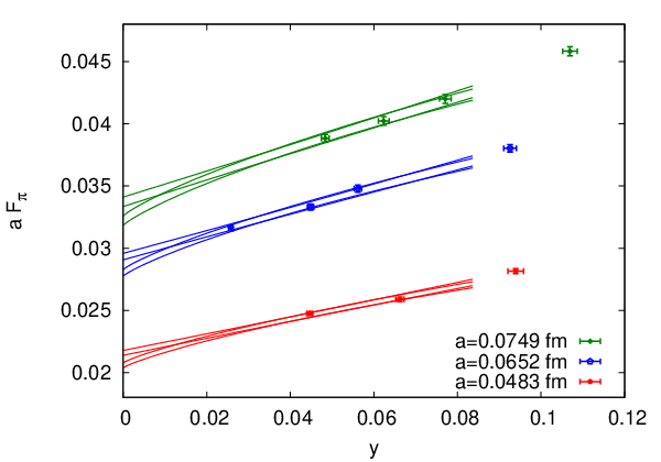
The numerical results for all lattices are reported in Table 4, and those for the pseudoscalar decay constant and for the cubic root of the ratio are shown in Fig. 5 versus . We fit to the function
| (26) |
where is common to all lattice spacings, restricted to the points with MeV (see left plot of Fig. 5). This function rests on the Symanzik expansion and is compatible with Wilson ChPT (WChPT) at the NLO [37]. To estimate the systematic error, we performed a number of fits to different functions: linear in with MeV, and next-to-next-to-leading order in ChPT with all data included. As a final result we quote , and at , and fm respectively, where the second (systematic) error takes into account the spread of the results from the various fits. By fixing the scale from , and by performing a continuum-limit extrapolation we obtain our final result MeV.
We further compute the ratio for all data points. We fit the data restricted to MeV to
| (27) |
where , and are common to all lattice spacings, and the fit function is again the one resting on the Symanzik expansion and compatible with WChPT at the NLO. Also in this case we checked several variants although the data look very flat up to the heaviest mass. From the fits we get , where the systematic error is determined as for . This translates to a value for the renormalisation-group-invariant dimensionless ratio of , which in turn corresponds to MeV if again is used to set the scale.

Appendix C Mode number in chiral perturbation theory
When chiral symmetry is spontaneously broken, the mode number can be computed in the chiral effective theory. At the NLO it reads [12] (see also Ref. [38])
| (28) |
where
| (29) |
The constants and are, respectively, the pion decay constant in the chiral limit and a SU low-energy effective coupling renormalized at the scale . The formula in Eq. (28) has some interesting properties:
- •
for
(30) and therefore at fixed the mode number has no chiral logs when ;
- •
since in the continuum the operator has a threshold at , the mode number must satisfy
(31) a property which is inherited by the NLO ChPT formula;
- •
in the chiral limit becomes independent on . This is an accident of the ChPT theory at NLO [29];
- •
the -dependence in the square brackets on the r.h.s. of (28) is parameter-free. Since , the behaviour of the function implies that is a decreasing function of at fixed , and no ambiguity is left due to free parameters.
At the NLO the effective spectral density defined in Eq. (5) reads
| (32) |
where
| (33) |
The quantity inherits the same peculiar properties of at NLO: at fixed and it has no chiral logarithms when , it is independent from and in the chiral limit, and at non-zero quark mass it is a decreasing parameter-free (apart the overall factor) function of . It is very weakly dependent on in the range we are interested in. To have a quantitative idea of the dependence of we can choose , MeV, MeV, MeV, MeV to obtain
| (34) |
For light values of the quark masses the variations are rather mild , i.e. of the order of few percent. The next-to-next-to leading corrections in are of the form . They are expected to spoil some of the peculiar properties of the NLO formula. In the chiral limit the corrections can induce a -dependence, and the can change the parameter-free dependence on within the square brackets on the r.h.s. of Eq. (32).
C.1 Finite volume effects
Finite volume effects in the mode number were computed in the chiral effective theory at the NLO in Refs. [12, 38] (see also [30]). They are given by
| (35) | |||||
where
| (36) |
with , , and is a modified Bessel function [39]. Furthermore, and denotes the sum over all integers without . By expanding the Bessel functions for large arguments [39], it is straightforward to show that the most significant terms in the sum on the r.h.s of Eq. (35) are proportional to the exponentials and , where and are the leading-order expressions in ChPT for the mass of a pseudoscalar meson made of two valence quarks of mass and respectively.
C.2 Discretization effects
At finite lattice spacing and volume, the threshold region should be treated carefully in ChPT [19]. The latter can be avoided by considering the quantity , with . In this case the computation in the GSM power-counting regime of the Wilson ChPT gives [30]
| (37) |
Since is expected to be negative [40, 20], if we rewrite
| (38) |
and we keep constant , then is a decreasing function of on the lattice too. At variance with the continuum case, however, a free parameter appears in the function, and its magnitude cannot be predicted. Remarkably is free from discretization effects in the chiral limit, and therefore it is independent on and . The continuum extrapolation of the chiral value of then removes the discretization effects due to the reference scale used.
Appendix D Numerical results for the mode number
We collect the results for the mode number in Tables 5, 6 and 7. For each lattice the values of correspond to approximatively 20, 25, 30, 40, 55, 71, 86, 101, 116 MeV with the exception of the lattice E5 for which also MeV were computed.
| id | |||
|---|---|---|---|
| A3 | 55 | 0.008673 | 13.3(6) |
| 0.009208 | 16.2(6) | ||
| 0.009821 | 20.5(7) | ||
| 0.011235 | 29.6(9) | ||
| 0.013665 | 47.3(10) | ||
| 0.016322 | 66.9(12) | ||
| 0.019110 | 88.2(14) | ||
| 0.021979 | 111.1(16) | ||
| 0.024901 | 134.6(18) | ||
| A4 | 55 | 0.006205 | 11.6(6) |
| 0.006929 | 15.9(7) | ||
| 0.007723 | 20.6(7) | ||
| 0.009447 | 30.8(8) | ||
| 0.012228 | 48.8(10) | ||
| 0.015127 | 68.6(12) | ||
| 0.018088 | 89.6(13) | ||
| 0.021085 | 110.9(15) | ||
| 0.024103 | 132.5(15) | ||
| A5 | 55 | 0.005352 | 11.4(6) |
| 0.006176 | 15.6(6) | ||
| 0.007054 | 20.6(7) | ||
| 0.008905 | 31.9(8) | ||
| 0.011810 | 50.1(11) | ||
| 0.014786 | 68.3(13) | ||
| 0.017799 | 88.7(14) | ||
| 0.020831 | 108.7(16) | ||
| 0.023877 | 129.2(18) | ||
| B6 | 50 | 0.004800 | 59.5(10) |
| 0.005703 | 82.5(11) | ||
| 0.006642 | 108.4(13) | ||
| 0.008580 | 162.3(16) | ||
| 0.011563 | 253.0(22) | ||
| 0.014586 | 346.5(25) | ||
| 0.017629 | 443(3) | ||
| 0.020683 | 543(3) | ||
| 0.023743 | 647(4) |
| id | |||
|---|---|---|---|
| D5 | 345 | 0.006720 | 2.09(9) |
| 0.007239 | 2.77(10) | ||
| 0.007826 | 3.42(10) | ||
| 0.009153 | 5.26(12) | ||
| 0.011385 | 8.38(16) | ||
| 0.013782 | 11.69(19) | ||
| 0.016271 | 15.16(22) | ||
| 0.018815 | 18.61(25) | ||
| 0.021396 | 22.3(3) | ||
| E5 | 92 | 0.006720 | 7.3(3) |
| 0.007239 | 9.3(3) | ||
| 0.007826 | 11.5(3) | ||
| 0.009153 | 17.1(4) | ||
| 0.011385 | 26.9(5) | ||
| 0.013782 | 37.4(7) | ||
| 0.016271 | 47.3(8) | ||
| 0.018815 | 58.0(9) | ||
| 0.021396 | 68.8(10) | ||
| 0.027499 | 93.7(10) | ||
| 0.036321 | 138.6(12) | ||
| 0.054110 | 259.7(16) | ||
| 0.089863 | 689(3) | ||
| F6 | 50 | 0.004618 | 34.7(9) |
| 0.005342 | 47.6(11) | ||
| 0.006111 | 60.7(12) | ||
| 0.007732 | 90.8(16) | ||
| 0.010268 | 135.8(17) | ||
| 0.012865 | 183.0(20) | ||
| 0.015492 | 230.9(23) | ||
| 0.018137 | 280(3) | ||
| 0.020791 | 330(3) | ||
| F7 | 50 | 0.004159 | 34.7(9) |
| 0.004950 | 47.0(10) | ||
| 0.005770 | 59.3(10) | ||
| 0.007464 | 87.1(12) | ||
| 0.010065 | 128.9(16) | ||
| 0.012701 | 172.0(21) | ||
| 0.015354 | 217.2(23) | ||
| 0.018015 | 265(3) | ||
| 0.020682 | 314(3) | ||
| G8 | 50 | 0.003737 | 113.7(16) |
| 0.004599 | 153.8(18) | ||
| 0.005472 | 196.7(22) | ||
| 0.007233 | 282.3(25) | ||
| 0.009892 | 409(3) | ||
| 0.012560 | 543(3) | ||
| 0.015233 | 682(4) | ||
| 0.017910 | 828(4) | ||
| 0.020587 | 981(5) |
| id | |||
|---|---|---|---|
| N5 | 60 | 0.005287 | 12.0(6) |
| 0.005647 | 15.6(6) | ||
| 0.006058 | 19.3(7) | ||
| 0.006998 | 27.3(8) | ||
| 0.008599 | 40.2(9) | ||
| 0.010334 | 52.3(10) | ||
| 0.012146 | 65.0(11) | ||
| 0.014005 | 77.7(12) | ||
| 0.015895 | 91.2(13) | ||
| N6 | 60 | 0.003797 | 11.0(4) |
| 0.004284 | 14.9(5) | ||
| 0.004812 | 18.3(5) | ||
| 0.005949 | 25.6(7) | ||
| 0.007765 | 37.3(8) | ||
| 0.009646 | 49.1(8) | ||
| 0.011562 | 60.4(9) | ||
| 0.013496 | 72.6(10) | ||
| 0.015444 | 85.8(11) | ||
| O7 | 50 | 0.003137 | 34.3(9) |
| 0.003710 | 45.9(10) | ||
| 0.004309 | 57.5(11) | ||
| 0.005548 | 78.5(12) | ||
| 0.007459 | 111.9(15) | ||
| 0.009399 | 147.8(16) | ||
| 0.011354 | 184.0(18) | ||
| 0.013316 | 220.8(19) | ||
| 0.015284 | 260.2(21) |
| 12.9 | 20.9 | 32.0 | |
|---|---|---|---|
| 22.7 | 0.0289(20) | 0.032(3) | 0.033(3) |
| 27.7 | 0.0249(21) | 0.023(3) | 0.029(3) |
| 35.3 | 0.0191(16) | 0.025(3) | 0.0308(24) |
| 47.9 | 0.0192(15) | 0.0239(22) | 0.0288(19) |
| 63.0 | 0.0221(15) | 0.0228(24) | 0.0229(18) |
| 78.2 | 0.0210(16) | 0.0174(20) | 0.0224(18) |
| 93.3 | 0.0212(14) | 0.0221(21) | 0.0211(18) |
| 108.4 | 0.0237(15) | 0.0257(22) | 0.0243(19) |
Appendix E Numerical analysis of discretization effects
In this appendix we report more details on the discretization effects that we have observed in our data. We limit ourselves to an empirical discussion of the results obtained by following the strategy described in Section 5.1.


A first look into the data reveals that discretization effects in show a non-trivial dependence on and . We plot the mode number at MeV, normalized with respect to its value at MeV, for all three lattice spacings and all values of in Figure 6, left hand side. After interpolating the effective spectral density in , we fit the data linearly in
| (39) |
for each pair of . By fitting linearly in (Figure 6, right plot)
| (40) |
for each , we obtain the values for shown in the left plot of Figure 7. Within errors, turns out to be compatible with a constant. To reduce the noise in , we repeat the fit in Eq. (40) but constraining to be a constant. The results of this fit are shown in the right plot of Figure 7. The coefficient tends to a constant for large , while a significant drop is observed towards the origin. In an intermediate range, the opposite signs of and allow for a compensation of the different effects, implying an effectively flat dependence of in the lattice spacing. Within the large errors, the mass-dependent discretization effects could be compatible with the functional form given in Eq. (37) [30]. The sign of the pole, however, appears to be opposite than predicted in Refs. [20, 40]. In this respect it must be said that it is not clear that the GSM power-counting scheme used in Ref. [30] applies in the range of parameters of our data.


References
- [1] M. Hasenbusch, Speeding up the hybrid Monte Carlo algorithm for dynamical fermions, Phys. Lett. B519 (2001) 177–182, [hep-lat/0107019].
- [2] M. Lüscher, Schwarz-preconditioned HMC algorithm for two-flavour lattice QCD, Comput. Phys. Commun. 165 (2005) 199–220, [hep-lat/0409106].
- [3] L. Del Debbio, L. Giusti, M. Lüscher, R. Petronzio, and N. Tantalo, QCD with light Wilson quarks on fine lattices (I): First experiences and physics results, JHEP 0702 (2007) 056, [hep-lat/0610059].
- [4] C. Urbach, K. Jansen, A. Shindler, and U. Wenger, HMC algorithm with multiple time scale integration and mass preconditioning, Comput. Phys. Commun. 174 (2006) 87–98, [hep-lat/0506011].
- [5] M. Lüscher and S. Schaefer, Lattice QCD with open boundary conditions and twisted-mass reweighting, Comput. Phys. Commun. 184 (2013) 519–528, [arXiv:1206.2809].
- [6] S. Aoki, Y. Aoki, C. Bernard, T. Blum, G. Colangelo, et. al., Review of lattice results concerning low-energy particle physics, Eur. Phys. J. C74 (2014), no. 9 2890, [arXiv:1310.8555].
- [7] S. Weinberg, Phenomenological Lagrangians, Physica A96 (1979) 327.
- [8] J. Gasser and H. Leutwyler, Chiral Perturbation Theory to One Loop, Ann. Phys. 158 (1984) 142.
- [9] T. Banks and A. Casher, Chiral Symmetry Breaking in Confining Theories, Nucl. Phys. B169 (1980) 103.
- [10] H. Leutwyler and A. V. Smilga, Spectrum of Dirac operator and role of winding number in QCD, Phys. Rev. D46 (1992) 5607–5632.
- [11] E. V. Shuryak and J. Verbaarschot, Random matrix theory and spectral sum rules for the Dirac operator in QCD, Nucl. Phys. A560 (1993) 306–320, [hep-th/9212088].
- [12] L. Giusti and M. Lüscher, Chiral symmetry breaking and the Banks-Casher relation in lattice QCD with Wilson quarks, JHEP 0903 (2009) 013, [arXiv:0812.3638].
- [13] G. P. Engel, L. Giusti, S. Lottini, and R. Sommer, Chiral condensate from the Banks-Casher relation, PoS LATTICE2013 (2014) 119, [arXiv:1309.4537].
- [14] G. P. Engel, Chiral condensate in QCD from the Banks-Casher relation, - Lattice 2014 - New York.
- [15] G. P. Engel, L. Giusti, S. Lottini, and R. Sommer, Chiral symmetry breaking in QCD Lite, arXiv:1406.4987.
- [16] L. Del Debbio, L. Giusti, M. Lüscher, R. Petronzio, and N. Tantalo, Stability of lattice QCD simulations and the thermodynamic limit, JHEP 02 (2006) 011, [hep-lat/0512021].
- [17] B. Sheikholeslami and R. Wohlert, Improved Continuum Limit Lattice Action for QCD with Wilson Fermions, Nucl. Phys. B259 (1985) 572.
- [18] M. Lüscher, S. Sint, R. Sommer, and P. Weisz, Chiral symmetry and O(a) improvement in lattice QCD, Nucl. Phys. B478 (1996) 365–400, [hep-lat/9605038].
- [19] P. Damgaard, K. Splittorff, and J. Verbaarschot, Microscopic Spectrum of the Wilson Dirac Operator, Phys. Rev. Lett. 105 (2010) 162002, [arXiv:1001.2937].
- [20] K. Splittorff and J. Verbaarschot, The Microscopic Twisted Mass Dirac Spectrum, Phys. Rev. D85 (2012) 105008, [arXiv:1201.1361].
- [21] L. Giusti and S. Necco, Spontaneous chiral symmetry breaking in QCD: A Finite-size scaling study on the lattice, JHEP 0704 (2007) 090, [hep-lat/0702013].
- [22] M. Marinkovic and S. Schaefer, Comparison of the mass preconditioned HMC and the DD-HMC algorithm for two-flavour QCD, PoS LATTICE2010 (2010) 031, [arXiv:1011.0911].
- [23] Lüscher, Martin, DD-HMC algorithm for two-flavour lattice QCD, http://luscher.web.cern.ch/luscher/DD-HMC/index.html.
- [24] P. Fritzsch, F. Knechtli, B. Leder, M. Marinkovic, S. Schaefer, et. al., The strange quark mass and Lambda parameter of two flavor QCD, Nucl. Phys. B865 (2012) 397–429, [arXiv:1205.5380].
- [25] ALPHA Collaboration, P. Fritzsch, P. Korcyl, B. Leder, S. Schaefer, H. Simma, R. Sommer, and F. Virotta in preparation.
- [26] M. Marinkovic, S. Schaefer, R. Sommer, and F. Virotta, Strange quark mass and Lambda parameter by the ALPHA collaboration, PoS LATTICE2011 (2011) 232, [arXiv:1112.4163].
- [27] ALPHA Collaboration, M. Bruno, S. Schaefer, and R. Sommer, Topological susceptibility and the sampling of field space in Nf = 2 lattice QCD simulations, JHEP 1408 (2014) 150, [arXiv:1406.5363].
- [28] ALPHA Collaboration, S. Schaefer, R. Sommer, and F. Virotta, Critical slowing down and error analysis in lattice QCD simulations, Nucl. Phys. B845 (2011) 93–119, [arXiv:1009.5228].
- [29] A. V. Smilga and J. Stern, On the spectral density of Euclidean Dirac operator in QCD, Phys. Lett. B318 (1993) 531–536.
- [30] S. Necco and A. Shindler, Spectral density of the Hermitean Wilson Dirac operator: a NLO computation in chiral perturbation theory, JHEP 1104 (2011) 031, [arXiv:1101.1778].
- [31] K. Cichy, E. Garcia-Ramos, and K. Jansen, Chiral condensate from the twisted mass Dirac operator spectrum, JHEP 1310 (2013) 175, [arXiv:1303.1954].
- [32] ALPHA collaboration Collaboration, K. Jansen and R. Sommer, O(a) improvement of lattice QCD with two flavors of Wilson quarks, Nucl. Phys. B530 (1998) 185–203, [hep-lat/9803017].
- [33] M. Della Morte, R. Hoffmann, and R. Sommer, Non-perturbative improvement of the axial current for dynamical Wilson fermions, JHEP 0503 (2005) 029, [hep-lat/0503003].
- [34] S. Sint and P. Weisz, Further results on O(a) improved lattice QCD to one loop order of perturbation theory, Nucl. Phys. B502 (1997) 251–268, [hep-lat/9704001].
- [35] S. Sint and P. Weisz, Further one loop results in O(a) improved lattice QCD, Nucl. Phys. Proc. Suppl. 63 (1998) 856–858, [hep-lat/9709096].
- [36] L. Del Debbio, L. Giusti, M. Lüscher, R. Petronzio, and N. Tantalo, QCD with light Wilson quarks on fine lattices. II. DD-HMC simulations and data analysis, JHEP 0702 (2007) 082, [hep-lat/0701009].
- [37] S. Aoki, O. Bar, and S. R. Sharpe, Vector and Axial Currents in Wilson Chiral Perturbation Theory, Phys. Rev. D80 (2009) 014506, [arXiv:0905.0804].
- [38] L. Giusti, “Spectral density of the QCD Dirac operator at the NLO in chiral perturbation theory” http://virgilio.mib.infn.it/ lgiusti/lgiusti.html, 2008.
- [39] M. Abramowitz and I. A. Stegun, Handbook of Mathematical Functions. Dover Publications, 1972.
- [40] M. T. Hansen and S. R. Sharpe, Constraint on the Low Energy Constants of Wilson Chiral Perturbation Theory, Phys. Rev. D85 (2012) 014503, [arXiv:1111.2404].