跳到论文正文
W Papers独立论文阅读器 arXiv:1411.6344 论文正文 计算阅读时间 · 0%
引用这篇论文根据当前论文元数据生成,正式投稿前建议核对。


License: arXiv.org perpetual non-exclusive license
arXiv:1411.6344v2 [hep-ph] 01 Apr 2015

Constraints on the septet-doublet mixing models from oblique parameters

Chao-Qiang Geng1,2,3, Lu-Hsing Tsai1, and Yao Yu3 Note: geng@phys.nthu.edu.tw Note: lhtsai@phys.nthu.edu.tw Note: yuyao@cqupt.edu.cn Affiliation: 1Chongqing University of Posts & Telecommunications, Chongqing, 400065, China
2Department of Physics, National Tsing Hua University, Hsinchu, 300, Taiwan
3Physics Division, National Center for Theoretical Sciences, Hsinchu, 300, Taiwan
August 24, 2026
Abstract

The limitations of the doublet-septet mixing models by the deviations of electroweak oblique parameters Δ​S\Delta S and Δ​T\Delta T are studied. In the minimal model, the mixture of the septet η\eta and the scalar doublet in the standard model (SM) is driven by a non-Hermitian dimension-7 operator. For a smaller bare mass of the septet, Δ​S\Delta S gives a stringent constraint on the mixing angle sin⁡β\sin\beta between the CP-odd neutral parts of the SM Higgs doublet and η\eta. In general, increasing the mass of the scalar septet MηM_{\eta} will enhance the deviation of TT from the SM, whereas it decreases the magnitude of Δ​S\Delta S for a larger bare mass within the range Mη≲400​GeVM_{\eta}\lesssim 400\,{\rm GeV}. We also examine two extended models from the ordinary doublet-septet mixture pattern. One of them is based on a inert doublet-septet mixing pattern, in which there is no vacuum expectation value for the neutral component of η\eta, and a stable dark matter could naturally exist. For a benchmark point with this inner doublet mass of Mχ=250M_{\chi}=250{\rm} and Mη=400​GeVM_{\eta}=400\,{\rm GeV} in this model, the mixing coefficient is found to be less than 1.81.8. The other extension is constructed by imposing a doubly charged scalar mixed with the doubly charged component of the septet. Apart from the contribution by the septet-doublet admixture, Δ​S\Delta S is suppressed by a factor of sW2s_{W}^{2} and Δ​T\Delta T has a significant constraint due to the vanishing vacuum polarization of ZZ at the momentum transfer p2=0p^{2}=0.

I Introduction

The discovery of the 125​GeV125\,{\rm GeV} Higgs boson makes the standard model (SM) complete [1, 2]. However, there is still a possibility that some fraction of this light boson comes from other unknown scalar particles, carrying quantum numbers (I,Y)(I,Y) under the gauge symmetry of SU​(2)L×U​(1)Y{\rm SU}(2)_{L}\times{\rm U}(1)_{Y}, for which the electric charge is related by Q=I3+Y/2Q=I_{3}+Y/2, where I3I_{3} is the third component the of weak isospin I=(n−1)/2I=(n-1)/2, with nn being the dimension of the representation for SU​(2)L{\rm SU}(2)_{L}. One example is to impose one or more scalar doublets with the quantum number (2,1)(2,1) [3, 4] or singlet (1,0)(1,0) [5, 6] to couple with the ordinary SM scalar doublet. It is interesting to note that the vacuum expectation value (VEV) of the singlet or doublet does not change the ρ\rho parameter from unity at tree level [7, 8], so that these types of the models can only be constrained by the electroweak oblique parameters of SS, TT, and UU [9, 10], in which S=−0.03±0.10S=-0.03\pm 0.10, T=0.01±0.12T=0.01\pm 0.12, and U=0.05±0.10U=0.05\pm 0.10 have been given by the recently global fitting [11]. In particular, it has been pointed out that the mixing angles in singlet-doublet mixing [12, 13], two Higgs doublet [14, 15, 16, 17], and multi-doublet [18, 19] models are bounded by SS and TT.

Besides the SU(2) singlet or doublet, there are a series of specific higher multiplets which can also retain ρ=1\rho=1, In particular, the SU(2) septet η\eta with Y=4Y=4 is the smallest choice of the multiplet to have the feature [20]. However, the septet with a nonzero VEV via the renormalizable operators is not allowed. Instead, some higher dimensional operators involving the septet and doublet are required to offer the mixings between them [21]. Although the VEV of the septet vηv_{\eta} is not limited by the ρ\rho parameter, electroweak oblique parameters could further constrain it to be vη≲20​GeVv_{\eta}\lesssim 20\,{\rm GeV} [22]. Furthermore, the Higgs-gauge and Higgs-fermion couplings observed from the LHC also restrict the structure of the septet [23, 24] with vη≲6​GeVv_{\eta}\lesssim 6\,{\rm GeV} [25].

There are also many applications for the scenarios that the extra multiplet cannot preserve the unity for ρ\rho. The value of ρ=1.0000±0.0009\rho=1.0000\pm 0.0009 [11] from the global fitting constrains the VEV of the multiplet up to order of several GeV, which means that the multiplet should be inert from the SM Higgs doublet, with only a tiny mixture allowed. The Higgs triplet model (Type-II seesaw) [26, 27, 28, 29, 30, 31, 32] is one of the typical example in which the VEV of the triplet is limited to be less than 𝒪⁡(1)\mathcal{O}(1) GeV [33, 34, 35, 36, 37]. The constraint on the VEV of the quintuplet (5,2)(5,2) was also studied [38]. For the extreme case that the VEV of the multiplet is forbidden by some discrete or continue symmetry, the oblique parameters can help to constrain the mixings of the multiplet with other particles. This type of the models can also contain dark matter if there exists a lightest component carrying a nonzero charge for the symmetry [39, 40, 41, 42, 43]. For more complicated situations, it is worth to explore the possibility that one or more scalar doublets and singlets mix with the septet.

This paper is organized as follows. In Sec. II, we review the septet-doublet mixing model and constrain the model from the oblique parameters. In Sec. III, we study the extended septet models. We give our conclusions in Sec. IV.

II The doubly-septet mixing model

It is known that the non-zero VEVs of new SU(2)×\timesU(1) multiplets with (n,Y)(n,Y) could contribute to ρ\rho with the general form [44]

ρ≡mW2mZ2​cW2=∑i[I(i)​(I(i)+1)−14​Y(i)2]​v(i)2∑i12​Y(i)2​v(i)2,\displaystyle\rho\equiv{m_{W}^{2}\over m_{Z}^{2}c_{W}^{2}}={\sum_{i}[I_{(i)}(I_{(i)}+1)-{1\over 4}Y_{(i)}^{2}]v_{(i)}^{2}\over\sum_{i}{1\over 2}Y_{(i)}^{2}v_{(i)}^{2}}\;, (1)

where the subscript (i)(i) indicates for the ii-th multiplet. From Eq. (1), it is easy to see that both singlet and doublet scalars as well as the septet η:(7,4)\eta:(7,4) will not change the ρ\rho parameter from unity. We would like to examine some models with the septet to keep ρ=1\rho=1 but constrained by the oblique parameters.

We start with a simple model in which η\eta acquires a non-zero VEV and has a mixing with the SM doublet. This model including two scalar components: the scalar doublet Φ=(Φ+,Φ0)T\Phi=(\Phi^{+}\;,\;\Phi^{0})^{T} in the SM, and the septet η\eta, which has the irreducible form consisting of seven independent complex components with the electric charges from Q=+5Q=+5 to −1-1, given by

η=(η(+5),η(+4),η(+3),η+⁣+,η+,η0,η−).\displaystyle\eta=(\eta^{(+5)}\;,\;\eta^{(+4)}\;,\;\eta^{(+3)}\;,\;\eta^{++}\;,\;\eta^{+}\;,\;\eta^{0}\;,\;\eta^{-})\;. (2)

The relevant terms of the scalar potential in this model are then given by

−L=−μ2(Φ∗Φ)+λ(Φ∗Φ)2+Mη2(η∗η)+[1Λ3ηΦ(Φ∗)5+H.c.],\displaystyle-L=-\mu^{2}(\Phi^{*}\Phi)+\lambda(\Phi^{*}\Phi)^{2}+M_{\eta}^{2}(\eta^{*}\eta)+\Big[{1\over\Lambda^{3}}\eta\Phi(\Phi^{*})^{5}+{\rm H.c.}\Big]\;, (3)

where the terms proportional to μ\mu and λ\lambda are the couplings in the SM, MηM_{\eta} is the bare mass of η\eta, and and Λ\Lambda is an effective energy scale. Note that the dimension-7 effective operator (1/Λ3)​η​Φ​(Φ∗)5(1/\Lambda^{3})\eta\Phi(\Phi^{*})^{5} in Eq. (3) is the simplest form of a higher dimensional operator containing a mixture of η\eta and Φ\Phi which can generate nonzero VEV for η\eta at the low energy scale [21]. Here, we also assume that there is no other lower dimensional effective operator. Other renormalizable gauge invariant terms such as (Φ∗​Φ​η∗​η)(\Phi^{*}\Phi\eta^{*}\eta) and (η​η​η∗​η∗\eta\eta\eta^{*}\eta^{*}) are not relevant in this paper and will be ignored in this study.

After the spontaneous symmetry broken due to the negative quadratic term of the scalar doublet, it leads to the VEV with Φ0=(vΦ+RΦ+i​IΦ)/2\Phi^{0}=(v_{\Phi}+R_{\Phi}+iI_{\Phi})/\sqrt{2}, and the the neutral part of the septet also acquires the VEV with η0=(vη+Rη+i​Iη)/2\eta^{0}=(v_{\eta}+R_{\eta}+iI_{\eta})/\sqrt{2} via the dimension-7 operator, with vΦv_{\Phi}(vηv_{\eta}), RΦR_{\Phi}(RηR_{\eta}), and IΦI_{\Phi}(IηI_{\eta}) being the VEV, CP-even component, and CP-odd component of Φ0\Phi^{0}(η0\eta^{0}), respectively. Then, we can take all mixing states of the doublet and septet into account, including neutral, singly charge, and doubly charged states. We discuss the mass spectrum of the septet by following the formulae in Ref. [21]. In general, the weak and mass eigenstates of the scalars can be expressed by

(RΦRη)=(cos⁡α−sin⁡αsin⁡αcos⁡α)​(hH),(IΦIη)=(cos⁡β−sin⁡βsin⁡βcos⁡β)​(G0A0),\displaystyle\left(\begin{array}[]{c}R_{\Phi}\\ R_{\eta}\\ \end{array}\right)=\left(\begin{array}[]{cc}\cos\alpha&-\sin\alpha\\ \sin\alpha&\cos\alpha\\ \end{array}\right)\left(\begin{array}[]{c}h\\ H\\ \end{array}\right)\;,\;\left(\begin{array}[]{c}I_{\Phi}\\ I_{\eta}\\ \end{array}\right)=\left(\begin{array}[]{cc}\cos\beta&-\sin\beta\\ \sin\beta&\cos\beta\\ \end{array}\right)\left(\begin{array}[]{c}G^{0}\\ A^{0}\\ \end{array}\right)\;,\;
(Φ+η+(η−)∗)=U​(G+η¯+S+),\displaystyle\left(\begin{array}[]{c}\Phi^{+}\\ \eta^{+}\\ (\eta^{-})^{*}\\ \end{array}\right)=U\left(\begin{array}[]{c}G^{+}\\ \bar{\eta}^{+}\\ S^{+}\\ \end{array}\right)\;,\;

where hh, HH, G0G^{0} and A0A^{0} are the neutral mass eigenstates; G+G^{+}, η¯+\bar{\eta}^{+} and S+S^{+} are the singly charged mass eigenstates; α\alpha and β\beta are the mixing angles11 1 After taking β→(π/2)−β\beta\rightarrow(\pi/2)-\beta and α→−α\alpha\rightarrow-\alpha, the notations become those in Ref. [21]. with tan⁡β=(4​vη)/vΦ\tan\beta=(4v_{\eta})/v_{\Phi}, and the 3×33\times 3 matrix UU is given by

U=(cβ0sβ104​sβ64−104​cβ−64​sβ10464​cβ).\displaystyle U=\left(\begin{array}[]{ccc}c_{\beta}&0&s_{\beta}\\ {\sqrt{10}\over 4}s_{\beta}&\sqrt{6}\over 4&-{\sqrt{10}\over 4}c_{\beta}\\ -{\sqrt{6}\over 4}s_{\beta}&\sqrt{10}\over 4&{\sqrt{6}\over 4}c_{\beta}\\ \end{array}\right)\;.

The mass spectra of the scalars are obtained as

Mh2\displaystyle M_{h}^{2} =\displaystyle= (1−32​tβtα)​Mη2,MH2=(1+32​tα​tβ)​Mη2,MA0=Mηcβ,\displaystyle(1-{3\over 2}{t_{\beta}\over t_{\alpha}})M_{\eta}^{2}\;,\;M_{H}^{2}=(1+{3\over 2}t_{\alpha}t_{\beta})M_{\eta}^{2}\;,\;M_{A^{0}}={M_{\eta}\over c_{\beta}}\;,
Mη¯±\displaystyle M_{\bar{\eta}^{\pm}} =\displaystyle= Mη,MS±=Mηcβ,\displaystyle M_{\eta}\;,\;M_{S^{\pm}}={M_{\eta}\over c_{\beta}}\;,\;
Mη+5\displaystyle M_{\eta^{+5}} =\displaystyle= Mη+4=Mη+3=Mη+2=Mη,\displaystyle M_{\eta^{+4}}=M_{\eta^{+3}}=M_{\eta^{+2}}=M_{\eta}\;,\; (28)

where sθ≡sin⁡θs_{\theta}\equiv\sin\theta, cθ≡cos⁡θc_{\theta}\equiv\cos\theta, and tθ≡tan⁡θt_{\theta}\equiv\tan\theta. The related details for the mass matrices are given in Appendix A. Without the mixing term η​Φ​(Φ∗)5\eta\Phi(\Phi^{*})^{5}, β\beta becomes zero and there is no mass splitting among the septet. Note that α\alpha can be determined once we take mh=125.7​GeVm_{h}=125.7\,{\rm GeV} [11] and fix sin⁡β\sin\beta. Subsequently, mHm_{H} can be evaluated too.

Recall that the definitions of SS, TT, and UU parameters are given by [45, 46]

S\displaystyle S =\displaystyle= 16​π​cW2​sW2e2​[ΠZ​Z​(MZ2)−ΠZ​Z​(0)MZ2−cW2−sW2cW​sW​∂Πγ​Z​(p2)∂(p2)|p2=0−∂Πγ​γ​(p2)∂(p2)|p2=0],\displaystyle{16\pi c_{W}^{2}s_{W}^{2}\over e^{2}}\Big[{\Pi_{ZZ}(M_{Z}^{2})-\Pi_{ZZ}(0)\over M_{Z}^{2}}-{c_{W}^{2}-s_{W}^{2}\over c_{W}s_{W}}{\partial\Pi_{\gamma Z}(p^{2})\over\partial(p^{2})}\Big|_{p^{2}=0}-{\partial\Pi_{\gamma\gamma}(p^{2})\over\partial(p^{2})}\Big|_{p^{2}=0}\Big]\;, (29)
T\displaystyle T =\displaystyle= 4​πe2​[ΠW​W​(0)MW2−ΠZ​Z​(0)MZ2],\displaystyle{4\pi\over e^{2}}\Big[{\Pi_{WW}(0)\over M_{W}^{2}}-{\Pi_{ZZ}(0)\over M_{Z}^{2}}\Big]\;, (30)
U\displaystyle U =\displaystyle= 16​π​sW2e2[ΠW​W​(MW2)−ΠW​W​(0)MW2−cW2ΠZ​Z​(MZ2)−ΠZ​Z​(0)MZ2\displaystyle{16\pi s_{W}^{2}\over e^{2}}\Big[{\Pi_{WW}(M_{W}^{2})-\Pi_{WW}(0)\over M_{W}^{2}}-c_{W}^{2}{\Pi_{ZZ}(M_{Z}^{2})-\Pi_{ZZ}(0)\over M_{Z}^{2}} (31)
−2cWsW∂Πγ​Z​(p2)∂(p2)|p2=0−sW2∂Πγ​γ​(p2)∂(p2)|p2=0],\displaystyle-2c_{W}s_{W}{\partial\Pi_{\gamma Z}(p^{2})\over\partial(p^{2})}\Big|_{p^{2}=0}-s_{W}^{2}{\partial\Pi_{\gamma\gamma}(p^{2})\over\partial(p^{2})}\Big|_{p^{2}=0}\Big]\;,

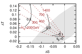
where Πa​b​(p2)\Pi_{ab}(p^{2}) are the coefficients of gμ​νg_{\mu\nu} for the vacuum polarizations of gauge bosons aa and bb (a,b=W,Z,γa,b=W,Z,\gamma) under the momentum transfer p2p^{2}. For Δ​U=0\Delta U=0, the deviation parameters of Δ​S\Delta S and Δ​T\Delta T from the data are Δ​S=0.00±0.08\Delta S=0.00\pm 0.08 and Δ​T=0.05±0.07\Delta T=0.05\pm 0.07 [11], respectively. We find that in this model |Δ​U||\Delta U| is typically smaller than |Δ​S||\Delta S| and |Δ​T||\Delta T| (see the expression of Δ​U\Delta U in Appendix B), with the order of 10−310^{-3} for Mη≳200​GeVM_{\eta}\gtrsim 200\,{\rm GeV} and sin⁡β≲0.3\sin\beta\lesssim 0.3, so that the assumption of Δ​U=0\Delta U=0 is viable. We show the formulae of Δ​S\Delta S and Δ​T\Delta T in Appendix B. Both of them only depend on MηM_{\eta} and tan⁡β\tan\beta, with the one-to-one correspondence in the interesting area of the S−TS-T plane, in the sense that there is no intersection among the curves with a constant MηM_{\eta} (or tan⁡β\tan\beta) as shown in Fig. 1. In general, Δ​S\Delta S is negative, whereas Δ​T\Delta T is always positive. Turning off the dimension-7 interaction (sin⁡β→0\sin\beta\rightarrow 0) will go back to an inert septet without a VEV, for which Δ​T=0\Delta T=0, while Δ​S\Delta S approaches zero for a large MηM_{\eta}. Notice that the allowed region by the observation at 90%90\%C.L. is positively correlated between Δ​S\Delta S and Δ​T\Delta T [11], so that for a larger value of MηM_{\eta} the restriction on sin⁡β\sin\beta does not become much more strongly despite its larger contribution to Δ​T\Delta T. As an example, we have sin⁡β≲0.21​(0.22)\sin\beta\lesssim 0.21(0.22) for Mη=200​(300)​GeVM_{\eta}=200(300)\,{\rm GeV}. We note that MηM_{\eta} is also limited by the experimental constraint from the pair production of η\eta, dominated by Drell-Yan processes, which is independent of vηv_{\eta} and sin⁡β\sin\beta. In Ref. [25], MηM_{\eta} is found to be larger than ∼400​GeV\sim 400\,{\rm GeV}. Similar results about the oblique parameters in this model were also discussed in Ref. [21]. We point out that our results for Δ​S\Delta S have two features which are different from those in Ref. [21] (see Eq. (68) in Appendix B). Firstly, we note that Δ​S\Delta S in our calculation is an increasing function of MηM_{\eta} within the range Mη≲400​GeVM_{\eta}\lesssim 400\,{\rm GeV}, and secondly, Δ​S≠0\Delta S\neq 0 when sin⁡β→0\sin\beta\rightarrow 0.

Refer to caption
Figure 1: Contours for MηM_{\eta} and tan⁡β\tan\beta in the Δ​S−Δ​T\Delta S-\Delta T plane, where the gray region corresponds to the global fitting results at 90%90\% C.L [11].

III Applications

III.1 Mixing between η:(7,4)\eta:(7,4) and χ:(2,1)\chi:(2,1)

We consider the model with an extra doublet χ=(χ+,12​(χR+i​χI))T\chi=(\chi^{+}\;,\;{1\over\sqrt{2}}(\chi_{R}+i\chi_{I}))^{T} besides the septet η\eta, where both scalars take odd charges under an Z2Z_{2} symmetry. The scalar potential can be written as

−L\displaystyle-L =\displaystyle= −μ2​(Φ∗​Φ)+λ​(Φ∗​Φ)2+Mχ2​(χ∗​χ)+λχ​(χ∗​χ)2,\displaystyle-\mu^{2}(\Phi^{*}\Phi)+\lambda(\Phi^{*}\Phi)^{2}+M_{\chi}^{2}(\chi^{*}\chi)+\lambda_{\chi}(\chi^{*}\chi)^{2}\;, (32)
+λ52[(Φ∗χ)2+h.c.]+Mη2(η∗η)+[CaΛ3ηχ(Φ∗)5+CbΛ3ηΦ(Φ∗)4χ∗+H.c.].\displaystyle+{\lambda_{5}\over 2}\Big[(\Phi^{*}\chi)^{2}+{\rm h.c.}\Big]+M_{\eta}^{2}(\eta^{*}\eta)+\Big[{C_{a}\over\Lambda^{3}}\eta\chi(\Phi^{*})^{5}+{C_{b}\over\Lambda^{3}}\eta\Phi(\Phi^{*})^{4}\chi^{*}+{\rm H.c.}\Big]\;.

Note that the Z2Z_{2} symmetry forbids the mixing of χ\chi or η\eta with the SM doublet Φ\Phi. Here, the quarter terms associated with (Φ∗​Φ)​χ∗​χ(\Phi^{*}\Phi)\chi^{*}\chi has been ignored, and the dimensional seven operators, η​χ​(Φ∗)5\eta\chi(\Phi^{*})^{5} and η​Φ​(Φ∗)4​χ∗\eta\Phi(\Phi^{*})^{4}\chi^{*}, are imposed to yield the mixing between χ\chi and η\eta. Without the last term in Eq. (32), the model will be reduced to the ordinary inert doublet one [47, 49, 48, 50, 51, 52, 53], in which the mass spectra are given by

M±2=Mχ2,MR2=Mχ2+λ52​v2,MI2=Mχ2−λ52​v2.\displaystyle M_{\pm}^{2}=M_{\chi}^{2}\;,\;M_{R}^{2}=M_{\chi}^{2}+{\lambda_{5}\over 2}v^{2}\;,\;M_{I}^{2}=M_{\chi}^{2}-{\lambda_{5}\over 2}v^{2}\;.\; (33)

The above masses turn into degeneracy when λ5\lambda_{5} approaches zero. The mass splittings inside χ\chi are the crucial quantities to give sizable contributions to TT or SS. The deviation of the TT parameter for the inert doublet is [49]

ΔT=116​π​mW2​sW2[F(M±2,MR2)+F(M±2,MI2)−F(MR2,MI2)].\displaystyle\Delta T={1\over 16\pi m_{W}^{2}s_{W}^{2}}[F(M_{\pm}^{2},M_{R}^{2})+F_{(}M_{\pm}^{2},M_{I}^{2})-F(M_{R}^{2},M_{I}^{2})]\;. (34)

where the definition of F⁡(x,y)F(x,y) is given in Appendix B. It is interesting to note that Δ​T\Delta T can be negative when there exists a large mass splitting between χR\chi_{R} and χI\chi_{I}, which is governed by MχM_{\chi} and λ5\lambda_{5}. Note that in this case η\eta only contributes to Δ​S\Delta S, but not to Δ​T\Delta T.

The next step is to take into account the interaction between χ\chi and η\eta. We separately study the effects on masses of neutral and singly charged states with some non-zero values of CaC_{a} and CbC_{b}, given by

Mx​12\displaystyle M_{x1}^{2} =\displaystyle= cos2⁡θxcos⁡(2​θx)​Mx2−sin2⁡θxcos⁡(2​θx)​Mη2,\displaystyle{\cos^{2}\theta_{x}\over\cos(2\theta_{x})}M_{x}^{2}-{\sin^{2}\theta_{x}\over\cos(2\theta_{x})}M_{\eta}^{2}\;,\;
Mx​22\displaystyle M_{x2}^{2} =\displaystyle= cos2⁡θxcos⁡(2​θx)​Mη2−sin2⁡θxcos⁡(2​θx)​Mx2,\displaystyle{\cos^{2}\theta_{x}\over\cos(2\theta_{x})}M_{\eta}^{2}-{\sin^{2}\theta_{x}\over\cos(2\theta_{x})}M_{x}^{2}\;, (35)

where Mx​1M_{x1} and Mx​2M_{x2} are two mass eigenvalues of χ\chi and η\eta, and θx\theta_{x} are mixing angles with x=R⁡(I)x=R(I) and ±\pm corresponding to the real(imaginary) part of the neutral and charged components, respectively. When taking the condition Mx<MηM_{x}<M_{\eta}, it is obvious that Mx​1<Mx​2M_{x1}<M_{x2}, which will be applied thereinafter. We list the mixing angles for two special cases as follows:

(i)\displaystyle(i) :\displaystyle: Ca≠0​ and ​Cb=0:\displaystyle C_{a}\neq 0\mbox{ and }C_{b}=0:
tan⁡(2​θR)=16​daMR2−Mη2​v2,tan⁡(2​θI)=−16​daMI2−Mη2​v2,tan⁡(2​θ±)=−daM±2−Mη2​v2;\displaystyle\tan(2\theta_{R})={{1\over\sqrt{6}}d_{a}\over M_{R}^{2}-M_{\eta}^{2}}v^{2}\;,\;\tan(2\theta_{I})={-{1\over\sqrt{6}}d_{a}\over M_{I}^{2}-M_{\eta}^{2}}v^{2}\;,\;\tan(2\theta_{\pm})={-d_{a}\over M_{\pm}^{2}-M_{\eta}^{2}}v^{2}\;;
(i​i)\displaystyle(ii) :\displaystyle: Ca=0​ and ​Cb≠0:\displaystyle C_{a}=0\mbox{ and }C_{b}\neq 0:
tan⁡(2​θR)=16​dbMR2−Mη2​v2,tan⁡(2​θI)=16​dbMI2−Mη2​v2,tan⁡(2​θ±)=115​dbM±2−Mη2​v2,\displaystyle\tan(2\theta_{R})={{1\over\sqrt{6}}d_{b}\over M_{R}^{2}-M_{\eta}^{2}}v^{2}\;,\;\tan(2\theta_{I})={{1\over\sqrt{6}}d_{b}\over M_{I}^{2}-M_{\eta}^{2}}v^{2}\;,\;\tan(2\theta_{\pm})={{1\over\sqrt{15}}d_{b}\over M_{\pm}^{2}-M_{\eta}^{2}}v^{2}\;,

where dj=(Cj​v3)/(8​Λ3)d_{j}=(C_{j}v^{3})/(\sqrt{8}\Lambda^{3}) for j=a,bj=a,b. The relevant coefficients in the above formulae can be found in Appendix A. Increasing the values of da,bd_{a,b} will also enlarge all the magnitudes of mixing angles between η\eta and χ\chi. For the limit of λ5→0\lambda_{5}\rightarrow 0, we find that |θR|=|θI|<|θ±||\theta_{R}|=|\theta_{I}|<|\theta_{\pm}| for (i), which means that MR​1=MI​1>M±1M_{R1}=M_{I1}>M_{\pm 1}, so that the lightest inert component is M±1M_{\pm 1}. Therefore, the stable neutral particle does not exist in this case. On the other hand, the existence of the stable charged scalar makes this scenario diafovored by experiments, unless we further impose some other effective operator to break the Z2Z_{2} symmetry. The situation for (ii) is opposite as |θR|=|θI|>|θ±||\theta_{R}|=|\theta_{I}|>|\theta_{\pm}| and MR​1=MI​1<M±1M_{R1}=M_{I1}<M_{\pm 1}, resulting in a stable DM. Notice that in the above discussion the mass splitting scale generated by the mixing is usually larger than the quantum corrections by gauge bosons (see Ref. [40]).

The explicit formulae for Δ​T\Delta T and Δ​S\Delta S are given in Appendix B. By fixing Mχ=250​GeVM_{\chi}=250\,{\rm GeV}, we plot them as functions of the coupling constant dbd_{b} for (ii) in Fig. 2. From the figure, we see that Δ​S\Delta S is always negative, whereas Δ​T\Delta T is positive. The magnitudes of Δ​T\Delta T raises with increasing dbd_{b}, and a larger MηM_{\eta} gives smaller Δ​S\Delta S and Δ​T\Delta T. For around 1.5​σ1.5\sigma deviation of an observed Δ​T\Delta T, that is, Δ​T<0.12\Delta T<0.12 [11], we have the upper bounds of db<1.5, 1.8d_{b}<1.5,\;1.8, and 2.12.1 for Mη=300, 400,M_{\eta}=300,\,400, and 500​GeV500\,{\rm GeV}, respectively. On the other hands, the constraint by Δ​S\Delta S is relatively weak.

Refer to caption
Figure 2: (a) Δ​S\Delta S and (b) Δ​T\Delta T as functions of dbd_{b} with Mχ=250​GeVM_{\chi}=250\,{\rm GeV} and different sets of mηm_{\eta}, where the horizontal dashed lines in (a) and (b) correspond to the 1.5−1.7​σ1.5-1.7\sigma bounds of Δ​S≥−0.08\Delta S\geq-0.08 and Δ​T≤0.12\Delta T\leq 0.12 [11], respectively.

III.2 Mixing between η:(7,4)\eta:(7,4) and ρ:(1,4)\rho:(1,4)

We now study the mixing of η\eta with a doubly-charge S​U​(2)LSU(2)_{L} singlet ρ:(1,4)\rho:(1,4), which can have the lepton number −2-2 due to the coupling with the charged lepton ρ​l¯Rc​lR\rho\bar{l}_{R}^{c}l_{R}. If η0\eta^{0} acquires a VEV and ρ\rho mixes with η+⁣+\eta^{++}, then the lepton number is broken. Majorana neutrino masses can be generated through a two-loop diagram involving the interaction ρ−⁣−​W+​W+\rho^{--}W^{+}W^{+} [54, 55, 56, 57, 58]. To mix ρ\rho and η\eta, like the scenario of the mixing between η\eta and Φ\Phi, some other higher dimensional operator are needed to achieve this goal in addition to the original one, η​Φ​(Φ5)∗\eta\Phi(\Phi^{5})^{*}, which gives a nonzero vηv_{\eta}. A dimension-8 operator ρ​η​Φ3​(Φ3)∗\rho\eta\Phi^{3}(\Phi^{3})^{*} is one of the possibility to drive the ρ−η\rho-\eta mixing. In this case, the potential is given by

−L\displaystyle-L =\displaystyle= −μ2​(Φ∗​Φ)+λ​(Φ∗​Φ)2+Mρ2​(ρ∗​ρ),\displaystyle-\mu^{2}(\Phi^{*}\Phi)+\lambda(\Phi^{*}\Phi)^{2}+M_{\rho}^{2}(\rho^{*}\rho)\;, (37)
+Mη2(η∗η)+[1Λ3ηΦ(Φ∗)5+1Λ′4ρη∗(Φ)3(Φ∗)3+H.c.],\displaystyle+M_{\eta}^{2}(\eta^{*}\eta)+\Big[{1\over\Lambda^{3}}\eta\Phi(\Phi^{*})^{5}+{1\over\Lambda^{\prime 4}}\rho\eta^{*}(\Phi)^{3}(\Phi^{*})^{3}+{\rm H.c.}\Big]\;,

where Λ′\Lambda^{\prime} is the mass scale related to the dimension-8 operator. Here, some of the quartic terms have been ignored. We will focus on the discussion of the effects on the oblique parameters by the mixing pattern independent of the source of the mixture.

The doubly-charge mixing can be parametrized as:

(ρ+⁣+η+⁣+)=(cos⁡θ−sin⁡θsin⁡θcos⁡θ)​(P1+⁣+P2+⁣+),\displaystyle\left(\begin{array}[]{c}\rho^{++}\\ \eta^{++}\\ \end{array}\right)=\left(\begin{array}[]{cc}\cos\theta&-\sin\theta\\ \sin\theta&\cos\theta\\ \end{array}\right)\left(\begin{array}[]{c}P_{1}^{++}\\ P_{2}^{++}\\ \end{array}\right)\;,\;

where θ\theta is the mixing angle and P1,2P_{1,2} are the two mass eigenstates. The mass eigenvalues are then derived directly by

MP12\displaystyle M_{P_{1}}^{2} =\displaystyle= cos2⁡θcos⁡(2​θ)​Mρ2−sin2⁡θcos⁡(2​θ)​Mη2,\displaystyle{\cos^{2}\theta\over\cos(2\theta)}M_{\rho}^{2}-{\sin^{2}\theta\over\cos(2\theta)}M_{\eta}^{2}\;,\;
MP22\displaystyle M_{P_{2}}^{2} =\displaystyle= cos2⁡θcos⁡(2​θ)​Mη2−sin2⁡θcos⁡(2​θ)​Mρ2.\displaystyle{\cos^{2}\theta\over\cos(2\theta)}M_{\eta}^{2}-{\sin^{2}\theta\over\cos(2\theta)}M_{\rho}^{2}\;. (45)

To study the influence on the electroweak structure, it is important to distinguish the deviations of the oblique parameters from different sources. Hence, The deviation of TT can be decomposed into two parts, Δ​T=Δ​T1+Δ​T2\Delta T=\Delta T_{1}+\Delta T_{2}, where Δ​T1\Delta T_{1} corresponds to the contribution from the η−Φ\eta-\Phi mixing, which is the same as the result in Eq. (B), while Δ​T2\Delta T_{2} is the rest given from the doubly-charge mixing, given by

Δ​T2\displaystyle\Delta T_{2} =\displaystyle= 14​π​sW2{15sβ2[sθ2K(MP12,MW2)+cθ2K(MP22,MW2)−K(Mη2,MW2)]\displaystyle{1\over 4\pi s_{W}^{2}}\Big\{15s_{\beta}^{2}[s_{\theta}^{2}K(M_{P_{1}}^{2},M_{W}^{2})+c_{\theta}^{2}K(M_{P_{2}}^{2},M_{W}^{2})-K(M_{\eta}^{2},M_{W}^{2})] (47)
+6mW2[sθ2F(MP12,Mη2)+cθ2F(MP22,Mη2)\displaystyle+{6\over m_{W}^{2}}\Big[s_{\theta}^{2}F(M_{P_{1}}^{2},M_{\eta}^{2})+c_{\theta}^{2}F(M_{P_{2}}^{2},M_{\eta}^{2})
+58​sβ2​(sθ2​F​(MP12,MW2)+cθ2​F​(MP22,MW2)−F⁡(Mη2,MW2))\displaystyle+{5\over 8}s_{\beta}^{2}(s_{\theta}^{2}F(M_{P_{1}}^{2},M_{W}^{2})+c_{\theta}^{2}F(M_{P_{2}}^{2},M_{W}^{2})-F(M_{\eta}^{2},M_{W}^{2}))
+38​(sθ2​F​(MP12,Mη¯±2)+cθ2​F​(MP22,Mη¯±2))\displaystyle+{3\over 8}(s_{\theta}^{2}F(M_{P_{1}}^{2},M_{\bar{\eta}^{\pm}}^{2})+c_{\theta}^{2}F(M_{P_{2}}^{2},M_{\bar{\eta}^{\pm}}^{2}))
+58cβ2(sθ2F(MP12,MS±2)+cθ2F(MP22,MS±2)−F(Mη2,MS±2))]}.\displaystyle+{5\over 8}c_{\beta}^{2}(s_{\theta}^{2}F(M_{P_{1}}^{2},M_{S^{\pm}}^{2})+c_{\theta}^{2}F(M_{P_{2}}^{2},M_{S^{\pm}}^{2})-F(M_{\eta}^{2},M_{S^{\pm}}^{2}))\Big]\Big\}\;.

The identical quantum numbers of I3I_{3} and YY between η+⁣+\eta^{++} and ρ+⁣+\rho^{++} make the relevant contribution to Δ​T\Delta T to be large because of the absence of F⁡(MP12,MP22)F(M_{P_{1}}^{2},M_{P_{2}}^{2}). As a result, the mass splitting of doubly-charge eigenstates is constrained stringently. Similarly, Δ​S=Δ​S1+Δ​S2\Delta S=\Delta S_{1}+\Delta S_{2}, where Δ​S1\Delta S_{1} is the same as Eq. (68), while Δ​S2\Delta S_{2} is given by

Δ​S2\displaystyle\Delta S_{2} =\displaystyle= −2π​(4​sW4)​[ξ⁡(M12MZ2,M12MZ2)+ξ⁡(M22MZ2,M22MZ2)−ξ⁡(Mη2MZ2,Mη2MZ2)].\displaystyle-{2\over\pi}(4s_{W}^{4})\Big[\xi({M_{1}^{2}\over M_{Z}^{2}},{M_{1}^{2}\over M_{Z}^{2}})+\xi({M_{2}^{2}\over M_{Z}^{2}},{M_{2}^{2}\over M_{Z}^{2}})-\xi({M_{\eta}^{2}\over M_{Z}^{2}},{M_{\eta}^{2}\over M_{Z}^{2}})\Big]\;. (48)

It is obvious that the contribution from Δ​S2\Delta S_{2} is tiny, because I3I_{3} is zero for both ρ±⁣±\rho^{\pm\pm} and η±⁣±\eta^{\pm\pm}, which makes the corresponding result proportional to sW4s_{W}^{4}.

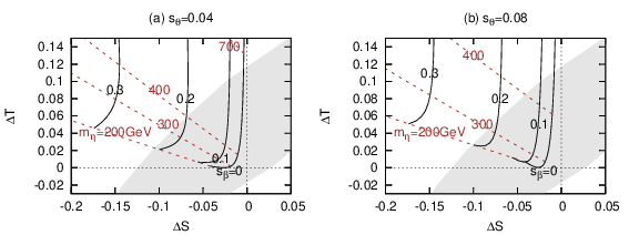
Our numerical results are shown in Fig. 3, where we have used sin⁡θ=0.04\sin\theta=0.04 and 0.080.08, together with Mρ=250​GeVM_{\rho}=250\,{\rm GeV} as illustrations. When MηM_{\eta} is large, say, Mη≳400​GeVM_{\eta}\gtrsim 400\,{\rm GeV}, Δ​T2\Delta T_{2} can yield a significant contribution to Δ​T\Delta T, so that the distortion in the S−TS-T plane appears, which is obvious in comparison with the ordinary figure in Fig. 1. For a larger value of sin⁡θ\sin\theta, the deformation is more apparent. Explicitly, we find that with Mη=400​GeVM_{\eta}=400\,{\rm GeV}, sin⁡β≲0.2​(0.15)\sin\beta\lesssim 0.2\,(0.15) for sin⁡θ=0.04​(0.08)\sin\theta=0.04\,(0.08).

Refer to caption
Figure 3: Contours of MηM_{\eta} and tan⁡β\tan\beta in the Δ​S−Δ​T\Delta S-\Delta T planes, for (a) sin⁡θ=0.04\sin\theta=0.04 and (b) sin⁡θ=0.08\sin\theta=0.08 with Mρ=250​GeVM_{\rho}={250{\rm GeV}}, where the gray region corresponds to the global fitting results at 90%90\% C.L [11].

IV Conclusions

We have studied the model including a mixing term between the SM Higgs doublet and an extra septet η:(7,4)\eta:(7,4) under SU​(2)L×U​(1)Y{\rm SU}(2)_{L}\times{\rm U}(1)_{Y}, which preserves the ρ\rho parameter to unity. The mixing between them arises from the effective dimension-7 operator η​Φ​(Φ∗)5\eta\Phi(\Phi^{*})^{5}. The possible parameter space has been explored by examining the electroweak oblique parameters. We have focused on the mass range Mη≲1500​GeVM_{\eta}\lesssim 1500\,{\rm GeV}. In general, Δ​S\Delta S is negative and increasing with MηM_{\eta} under the range of Mη≲400​GeVM_{\eta}\lesssim 400\,{\rm GeV}, whereas Δ​T\Delta T is always positive and increasing for a large sin⁡β\sin\beta. Basically, the constraint on sin⁡β\sin\beta changes slowly for different values of MηM_{\eta}. In the future, the global fitting of the oblique parameters could help to determine MηM_{\eta} and tan⁡β\tan\beta more precisely or directly exclude this model.

Besides the minimal doublet-septet mixing model, two extensions have been also discussed. One of them is to create an Z2Z_{2} odd sector which consists of the septet and an additional doublet χ\chi. Only two dimension-7 operators are possible to generate the mixing between η\eta and χ\chi. We have examined the effects of η​Φ​(Φ∗)4​χ∗\eta\Phi(\Phi^{*})^{4}\chi^{*} on the scalar mass spectra and oblique parameters. In particular, we have found the mixing coefficient db≲1.8d_{b}\lesssim 1.8 for Mη=400​GeVM_{\eta}=400\,{\rm GeV} and Mχ=250​GeVM_{\chi}=250\,{\rm GeV}. This result can help us to distinguish different mixing patterns by future analyses. The other extension is to have an additional admixture between the septet and an SU(2) singlet ρ:(1,4)\rho:(1,4). We can limit the mixing angle sin⁡θ\sin\theta in this kind of the models. For example, we have found that sin⁡β≲0.15\sin\beta\lesssim 0.15 for Mρ=250​GeVM_{\rho}=250\,{\rm GeV}, sin⁡θ=0.08\sin\theta=0.08, and Mη=400​GeVM_{\eta}=400\,{\rm GeV}, where the dominant constraint comes from Δ​T\Delta T. The existence of this kind of the mixing pattern could also be tested by the oncoming experiments.

Acknowledgements.
This work was supported by National Center for Theoretical Sciences, National Science Council (Grant No. NSC-101-2112-M-007-006-MY3) and National Tsing Hua University (Grant No. 104N2724E1).

Appendix A Mixing matrices for doublet-septet mixing model

To calculate the mass spectra in the doublet-septet mixing model, the first step is to deal with the non-hermitian effective coupling, which can be expanded as

η​Φ​(Φ∗)5+H.c.\displaystyle\eta\Phi(\Phi^{*})^{5}+{\rm H.c.} =\displaystyle= η(+5)​Φ0​(Φ∗⁣+)5+16​η(+4)​[−(Φ+∗)5​Φ++5​(Φ+⁣∗)4​Φ0]\displaystyle\eta^{(+5)}\Phi^{0}(\Phi^{*+})^{5}+{1\over\sqrt{6}}\eta^{(+4)}[-({\Phi^{+}}^{*})^{5}\Phi^{+}+5(\Phi^{+*})^{4}\Phi^{0}] (49)
+115​η+3​[−5​(Φ+∗)4​(Φ0∗)​Φ++10​(Φ+∗)3​(Φ0∗)2​Φ0]\displaystyle+{1\over\sqrt{15}}\eta^{+3}[-5({\Phi^{+}}^{*})^{4}({\Phi^{0}}^{*})\Phi^{+}+10({\Phi^{+}}^{*})^{3}({\Phi^{0}}^{*})^{2}\Phi^{0}]
+120​η+⁣+​[−10​(Φ+∗)3​(Φ0∗)2​Φ++10​(Φ+∗)2​(Φ0∗)3​Φ0]\displaystyle+{1\over\sqrt{20}}\eta^{++}[-10({\Phi^{+}}^{*})^{3}({\Phi^{0}}^{*})^{2}\Phi^{+}+10({\Phi^{+}}^{*})^{2}({\Phi^{0}}^{*})^{3}\Phi^{0}]
+115​η+​[−10​(Φ+∗)2​(Φ0∗)3​Φ++5​(Φ+∗)​(Φ0∗)4​Φ0]\displaystyle+{1\over\sqrt{15}}\eta^{+}[-10({\Phi^{+}}^{*})^{2}({\Phi^{0}}^{*})^{3}\Phi^{+}+5({\Phi^{+}}^{*})({\Phi^{0}}^{*})^{4}\Phi^{0}]
+16η0[−5(Φ+∗)(Φ0∗)4Φ++(Φ0∗)5Φ0]−η−(Φ0∗)5Φ++h.c.\displaystyle+{1\over\sqrt{6}}\eta^{0}[-5({\Phi^{+}}^{*})({\Phi^{0}}^{*})^{4}\Phi^{+}+({\Phi^{0}}^{*})^{5}\Phi^{0}]-\eta^{-}(\Phi^{0*})^{5}\Phi^{+}+{\rm h.c.}
∼\displaystyle\sim 515η+Φ+∗Φ0(Φ0∗)4+16η0Φ0(Φ0∗)5−η−Φ+(Φ0∗)5\displaystyle{5\over\sqrt{15}}\eta^{+}{\Phi^{+}}^{*}\Phi^{0}({\Phi^{0}}^{*})^{4}+{1\over\sqrt{6}}\eta^{0}\Phi^{0}(\Phi^{0*})^{5}-\eta^{-}\Phi^{+}({\Phi^{0}}^{*})^{5}
−56​η0​(Φ+∗)​(Φ0∗)4​Φ++H.c.,\displaystyle-{5\over\sqrt{6}}\eta^{0}({\Phi^{+}}^{*})({\Phi^{0}}^{*})^{4}\Phi^{+}+{\rm H.c.}\;,

where we have only shown the relevant terms to provide the quadratic mixings of η\eta and Φ\Phi after the spontaneous symmetry breaking. The tadpole conditions in the potential are

−μ2​vΦ+λ​vΦ3+126​(2)7​Λ3​vη​vΦ5=0,\displaystyle-\mu^{2}v_{\Phi}+\lambda v_{\Phi}^{3}+{12\over\sqrt{6}(\sqrt{2})^{7}\Lambda^{3}}v_{\eta}v_{\Phi}^{5}=0\;,
Mη2​vη+26​(2)7​Λ3​vΦ6=0.\displaystyle M_{\eta}^{2}v_{\eta}+{2\over\sqrt{6}(\sqrt{2})^{7}\Lambda^{3}}v_{\Phi}^{6}=0\;. (50)

The mixing matrix of the imaginary part is

Mη2​(16​vη2vΦ2−4​vηvΦ−4​vηvΦ0).\displaystyle M_{\eta}^{2}\left(\begin{array}[]{cc}{16v_{\eta}^{2}\over v_{\Phi}^{2}}&-{4v_{\eta}\over v_{\Phi}}\\ -{4v_{\eta}\over v_{\Phi}}&0\\ \end{array}\right)\;.

By comparing it with Eq. (II), we obtain the relation tβ=4​vη/vΦt_{\beta}={4v_{\eta}/v_{\Phi}} and the eigenvalues 00 and Mη2/cβ2M_{\eta}^{2}/c_{\beta}^{2}. Similarly, the mass matrix of the neutral part is

(2​λ​cβ2​v2−32​Mη2​tβ2−32​tβ​Mη2−32​tβ​Mη2Mη2).\displaystyle\left(\begin{array}[]{cc}2\lambda c_{\beta}^{2}v^{2}-{3\over 2}M_{\eta}^{2}t_{\beta}^{2}&-{3\over 2}t_{\beta}M_{\eta}^{2}\\ -{3\over 2}t_{\beta}M_{\eta}^{2}&M_{\eta}^{2}\\ \end{array}\right)\;.

From Eqs. (II) and  (A), we get two relations:

Mh2​sα2+MH2​cα2=Mη2,cα​sα​(Mh2−MH2)=−32​Mη2​tβ,\displaystyle M_{h}^{2}s_{\alpha}^{2}+M_{H}^{2}c_{\alpha}^{2}=M_{\eta}^{2}\;,\;c_{\alpha}s_{\alpha}(M_{h}^{2}-M_{H}^{2})=-{3\over 2}M_{\eta}^{2}t_{\beta}\;,\; (57)

which lead to the expressions of Mh2M_{h}^{2} and MH2M_{H}^{2} shown in Eq. (28).

The singly-charge mass matrix in the weak basis {Φ+,η+,(η−)∗}\{\Phi^{+}\;,\;\eta^{+}\;,\;(\eta^{-})^{*}\} is given by

Mη2​(tβ2−104​tβ64​tβ−104​tβ1064​tβ01).\displaystyle M_{\eta}^{2}\left(\begin{array}[]{ccc}t_{\beta}^{2}&-{\sqrt{10}\over 4}t_{\beta}&{\sqrt{6}\over 4}t_{\beta}\\ -{\sqrt{10}\over 4}t_{\beta}&1&0\\ {\sqrt{6}\over 4}t_{\beta}&0&1\\ \end{array}\right)\;.

The three eigenvalues of the matrix in Eq. (A) are MG±2=0M_{G^{\pm}}^{2}=0, Mη¯±2=Mη2M_{\bar{\eta}^{\pm}}^{2}=M_{\eta}^{2}, and MS±2=Mη2/cβ2M_{S^{\pm}}^{2}=M_{\eta}^{2}/c_{\beta}^{2} with the transformation matrix

U=(cβ0sβ104​sβ64−104​cβ−64​sβ10464​cβ).\displaystyle U=\left(\begin{array}[]{ccc}c_{\beta}&0&s_{\beta}\\ {\sqrt{10}\over 4}s_{\beta}&{\sqrt{6}\over 4}&-{\sqrt{10}\over 4}c_{\beta}\\ -{\sqrt{6}\over 4}s_{\beta}&{\sqrt{10}\over 4}&{\sqrt{6}\over 4}c_{\beta}\\ \end{array}\right)\;.

We now show the mixing pattern between the inert doublet and septet discussed in Sec. 3. We have two types of the mixing models: (i) η​χ​(Φ∗)5\eta\chi(\Phi^{*})^{5}, and (ii) η​Φ​(Φ∗)4​χ∗\eta\Phi(\Phi^{*})^{4}\chi^{*}. Like the procedure in the beginning of this section, we extract the terms relevant to the χ−η\chi-\eta mixing for (i) and (ii):

(i):η​χ​(Φ∗)5+h.c.∼16​η0​(χ0)​(Φ0)∗5−η−​(χ+)​(Φ0)∗5+H.c.,\displaystyle(i):\;\;\eta\chi(\Phi^{*})^{5}+{\rm h.c.}\sim{1\over\sqrt{6}}\eta^{0}(\chi^{0}){(\Phi^{0})^{*}}^{5}-\eta^{-}(\chi^{+}){(\Phi^{0})^{*}}^{5}+{\rm H.c.}\;, (66)
(i​i):η​Φ​(Φ∗)4​χ∗+h.c.∼16​η0​(χ0)∗​Φ0​(Φ0)∗4+115​η−​(χ+)∗​Φ0​(Φ0)∗4+H.c..\displaystyle(ii):\;\;\eta\Phi(\Phi^{*})^{4}\chi^{*}+{\rm h.c.}\sim{1\over\sqrt{6}}\eta^{0}(\chi^{0})^{*}\Phi^{0}{(\Phi^{0})^{*}}^{4}+{1\over\sqrt{15}}\eta^{-}(\chi^{+})^{*}\Phi^{0}{(\Phi^{0})^{*}}^{4}+{\rm H.c.}\;. (67)

Then, the relations in Eq. () can be obtained directly.

Appendix B oblique parameters Δ​S\Delta S and Δ​T\Delta T

In the doublet-septet mixing model, Δ​S\Delta S is given by

Δ​S\displaystyle\Delta S =\displaystyle= −2π[((3cW2−2sW2)2+(2cW2−2sW2)2+(cW2−2sW2)2+4sW4)ξ(Mη2MZ2,Mη2MZ2)\displaystyle-{2\over\pi}\Big[\Big((3c_{W}^{2}-2s_{W}^{2})^{2}+(2c_{W}^{2}-2s_{W}^{2})^{2}+(c_{W}^{2}-2s_{W}^{2})^{2}+4s_{W}^{4}\Big)\xi\Big({M_{\eta}^{2}\over M_{Z}^{2}},{M_{\eta}^{2}\over M_{Z}^{2}}\Big) (68)
+(32−sW2)2ξ(Mη¯±2MZ2,Mη¯±2MZ2)+(12−sW2)2ξ(MS±2MZ2,MS±2MZ2)]\displaystyle+\Big({3\over 2}-s_{W}^{2}\Big)^{2}\xi\Big({M_{\bar{\eta}^{\pm}}^{2}\over M_{Z}^{2}},{M_{\bar{\eta}^{\pm}}^{2}\over M_{Z}^{2}}\Big)+\Big({1\over 2}-s_{W}^{2}\Big)^{2}\xi\Big({M_{S^{\pm}}^{2}\over M_{Z}^{2}},{M_{S^{\pm}}^{2}\over M_{Z}^{2}}\Big)\Big]
−2π[152sβ2ξ(MW2MZ2,Mη¯±2MZ2)+152cβ2ξ(Mη¯±2MZ2,MS±2MZ2)\displaystyle-{2\over\pi}\Big[{15\over 2}s_{\beta}^{2}\xi\Big({M_{W}^{2}\over M_{Z}^{2}},{M_{\bar{\eta}^{\pm}}^{2}\over M_{Z}^{2}}\Big)+{15\over 2}c_{\beta}^{2}\xi\Big({M_{\bar{\eta}^{\pm}}^{2}\over M_{Z}^{2}},{M_{S^{\pm}}^{2}\over M_{Z}^{2}}\Big)
+14​(((cα​cβ+4​sα​sβ)2−1)​ξ​(Mh2MZ2,1)+(cα​sβ−4​sα​cβ)2​ξ​(Mh2MZ2,MA2MZ2)CLOSE\displaystyle+{1\over 4}\Big(((c_{\alpha}c_{\beta}+4s_{\alpha}s_{\beta})^{2}-1)\xi\Big({M_{h}^{2}\over M_{Z}^{2}},1\Big)+(c_{\alpha}s_{\beta}-4s_{\alpha}c_{\beta})^{2}\xi\Big({M_{h}^{2}\over M_{Z}^{2}},{M_{A}^{2}\over M_{Z}^{2}}\Big)
+(sαcβ−4cαsβ)2ξ(MH2MZ2,1)+(sαsβ+4cαcβ)2ξ(MH2MZ2,MA2MZ2))]\displaystyle+(s_{\alpha}c_{\beta}-4c_{\alpha}s_{\beta})^{2}\xi\Big({M_{H}^{2}\over M_{Z}^{2}},1\Big)+(s_{\alpha}s_{\beta}+4c_{\alpha}c_{\beta})^{2}\xi\Big({M_{H}^{2}\over M_{Z}^{2}},{M_{A}^{2}\over M_{Z}^{2}}\Big)\Big)\Big]
−13​π[12logMη2−34logMη¯±2+14logMS±2−154sβ2log(MW2Mη¯±2)−154cβ2log(Mη¯±2MS±2)\displaystyle-{1\over 3\pi}\Big[12\log{M_{\eta}^{2}}-{3\over 4}\log{M_{\bar{\eta}^{\pm}}^{2}}+{1\over 4}\log{M_{S^{\pm}}^{2}}-{15\over 4}s_{\beta}^{2}\log({M_{W}^{2}M_{\bar{\eta}^{\pm}}^{2}})-{15\over 4}c_{\beta}^{2}\log(M_{\bar{\eta}^{\pm}}^{2}M_{S^{\pm}}^{2})
−18​((cα​cβ+4​sα​sβ)2−1)​log⁡(Mh2​MZ2)−18​(cα​sβ−4​sα​cβ)2​log⁡(Mh2​MA2)\displaystyle-{1\over 8}((c_{\alpha}c_{\beta}+4s_{\alpha}s_{\beta})^{2}-1)\log(M_{h}^{2}M_{Z}^{2})-{1\over 8}(c_{\alpha}s_{\beta}-4s_{\alpha}c_{\beta})^{2}\log(M_{h}^{2}M_{A}^{2})
−18(sαcβ−4cαsβ)2log(MH2MZ2)−18(sαsβ+4cαcβ)2log(MH2MA2)]\displaystyle-{1\over 8}(s_{\alpha}c_{\beta}-4c_{\alpha}s_{\beta})^{2}\log(M_{H}^{2}M_{Z}^{2})-{1\over 8}(s_{\alpha}s_{\beta}+4c_{\alpha}c_{\beta})^{2}\log(M_{H}^{2}M_{A}^{2})\Big]
+1π[30sβ2cW2ζ(Mη¯±2MZ2,MW2MZ2)+[(cαcβ+4sαsβ)2−1]ζ(Mh2MZ2,1)\displaystyle+{1\over\pi}\Big[30s_{\beta}^{2}c_{W}^{2}\zeta\Big({M_{\bar{\eta}^{\pm}}^{2}\over M_{Z}^{2}},{M_{W}^{2}\over M_{Z}^{2}}\Big)+[(c_{\alpha}c_{\beta}+4s_{\alpha}s_{\beta})^{2}-1]\zeta\Big({M_{h}^{2}\over M_{Z}^{2}},1\Big)
+(−sαcβ+4cαsβ)2ζ(MH2MZ2,1)],\displaystyle+(-s_{\alpha}c_{\beta}+4c_{\alpha}s_{\beta})^{2}\zeta\Big({M_{H}^{2}\over M_{Z}^{2}},1\Big)\Big]\;,

where [46]

ξ⁡(x,y)\displaystyle\xi(x,y) =\displaystyle= 49−512​(x+y)+16​(x−y)2+14​[x2−y2−13​(x−y)3−x2+y2x−y]​log⁡xy\displaystyle{4\over 9}-{5\over 12}(x+y)+{1\over 6}(x-y)^{2}+{1\over 4}\Big[x^{2}-y^{2}-{1\over 3}(x-y)^{3}-{x^{2}+y^{2}\over x-y}\Big]\log{x\over y} (69)
−112​Δ​(x,y)​f​(x,y),\displaystyle-{1\over 12}\Delta(x,y)f(x,y)\;,
ζ⁡(x,y)\displaystyle\zeta(x,y) =\displaystyle= 12​[x−y−x+yx−y]​log⁡xy−1−12​f​(x,y),\displaystyle{1\over 2}\Big[{x-y}-{x+y\over x-y}\Big]\log{x\over y}-1-{1\over 2}f(x,y)\;, (70)
Δ⁡(x,y)\displaystyle\Delta(x,y) =\displaystyle= −1+2​(x+y)−(x−y)2,\displaystyle-1+2(x+y)-(x-y)^{2}\;, (71)
f⁡(x,y)={−2​Δ⁡(x,y)​(tan−1⁡x−y+1Δ⁡(x,y)−tan−1⁡x−y−1Δ⁡(x,y)) for ​Δ​(x,y)>0,0 for ​Δ​(x,y)=0,−Δ⁡(x,y)​log⁡x+y−1+−Δ⁡(x,y)x+y−1−−Δ⁡(x,y) for ​Δ​(x,y)<0.\displaystyle f(x,y)=\left\{\begin{array}[]{lc}-2\sqrt{\Delta(x,y)}\Big(\tan^{-1}{x-y+1\over\sqrt{\Delta(x,y)}}-\tan^{-1}{x-y-1\over\sqrt{\Delta(x,y)}}\Big)&\mbox{ for }\Delta(x,y)>0\;,\\ 0&\mbox{ for }\Delta(x,y)=0\;,\\ \sqrt{-\Delta(x,y)}\log{x+y-1+\sqrt{-\Delta(x,y)}\over x+y-1-\sqrt{-\Delta(x,y)}}&\mbox{ for }\Delta(x,y)<0\;.\end{array}\right.

Note that the above formula for Δ​S\Delta S is different from that given in Ref. [21]. In comparison with the formulae in Ref. [21], we have one additional contribution from the first term in Eq. (68), which decreases with a larger value of MηM_{\eta}, but it is dominated when sin⁡β\sin\beta is small. However, the result in Ref. [21] could be compatible with ours when MηM_{\eta} is not too small. It is easily checked that when sin⁡β→0\sin\beta\rightarrow 0, our result of Δ​S\Delta S from Eq. (68) is nonzero, whereas Δ​S→0\Delta S\rightarrow 0 in Ref. [21]. Δ​T\Delta T is found to be [21]

Δ​T\displaystyle\Delta T =\displaystyle= 14​π​sW2​MW2{14((cαcβ+4sαsβ)2−1)(G(Mh2,MW2)−G(Mh2,MZ2))\displaystyle{1\over 4\pi s_{W}^{2}M_{W}^{2}}\Big\{{1\over 4}((c_{\alpha}c_{\beta}+4s_{\alpha}s_{\beta})^{2}-1)(G(M_{h}^{2},M_{W}^{2})-G(M_{h}^{2},M_{Z}^{2}))
+14​(−sα​cβ+4​cα​sβ)2​(G⁡(MH2,MW2)−G⁡(MH2,MZ2))\displaystyle+{1\over 4}(-s_{\alpha}c_{\beta}+4c_{\alpha}s_{\beta})^{2}(G(M_{H}^{2},M_{W}^{2})-G(M_{H}^{2},M_{Z}^{2}))
−15​sβ24(G(Mη2,MW2)−G(Mη2,MZ2))],\displaystyle-{15s_{\beta}^{2}\over 4}(G(M_{\eta}^{2},M_{W}^{2})-G(M_{\eta}^{2},M_{Z}^{2}))\Big]\;,

where

G⁡(x,y)\displaystyle G(x,y) =\displaystyle= F⁡(x,y)+4​y​K​(x,y),\displaystyle F(x,y)+4yK(x,y)\;,\; (77)
F⁡(x,y)\displaystyle F(x,y) =\displaystyle= x+y2−x​yx−y​log⁡xy,K⁡(x,y)=x​log⁡x−y​log⁡yx−y.\displaystyle{x+y\over 2}-{xy\over x-y}\log{x\over y}\;,\;K(x,y)={x\log x-y\log y\over x-y}\;.\; (78)

In this model, Δ​U\Delta U is given by

Δ​U\displaystyle\Delta U =\displaystyle= 2π[((3cW2−2sW2)2+(2cW2−2sW2)2+(cW2−2sW2)2+(−2sW2)2)ξ(Mη2MZ2,Mη2MZ2)−76log(Mη4)\displaystyle{2\over\pi}\Big[\Big((3c_{W}^{2}-2s_{W}^{2})^{2}+(2c_{W}^{2}-2s_{W}^{2})^{2}+(c_{W}^{2}-2s_{W}^{2})^{2}+(-2s_{W}^{2})^{2}\Big)\xi\Big({M_{\eta}^{2}\over M_{Z}^{2}},{M_{\eta}^{2}\over M_{Z}^{2}}\Big)-{7\over 6}\log(M_{\eta}^{4}) (79)
+(32−sW2)2​log⁡(Mη¯2MZ2,Mη¯2MZ2)−316​log⁡(Mη¯4)+(12−sW2)2​ξ​(MS2MZ2,MS2MZ2)−148​log⁡(MS4)\displaystyle+({3\over 2}-s_{W}^{2})^{2}\log\Big({M_{\bar{\eta}}^{2}\over M_{Z}^{2}},{M_{\bar{\eta}}^{2}\over M_{Z}^{2}}\Big)-{3\over 16}\log(M_{\bar{\eta}}^{4})+({1\over 2}-s_{W}^{2})^{2}\xi\Big({M_{S}^{2}\over M_{Z}^{2}},{M_{S}^{2}\over M_{Z}^{2}}\Big)-{1\over 48}\log(M_{S}^{4})
+152​sβ2​(ξ⁡(MW2MZ2,Mη¯2MZ2)−2​cW2​ζ​(MW2MZ2,Mη¯2MZ2)−112​log⁡(MW2​Mη¯2))\displaystyle+{15\over 2}s_{\beta}^{2}\Big(\xi\Big({M_{W}^{2}\over M_{Z}^{2}},{M_{\bar{\eta}}^{2}\over M_{Z}^{2}}\Big)-2c_{W}^{2}\zeta\Big({M_{W}^{2}\over M_{Z}^{2}},{M_{\bar{\eta}}^{2}\over M_{Z}^{2}}\Big)-{1\over 12}\log(M_{W}^{2}M_{\bar{\eta}}^{2})\Big)
+152cβ2(ξ(Mη¯2MZ2,MS2MZ2)−112log(MS2Mη¯2))]\displaystyle+{15\over 2}c_{\beta}^{2}\Big(\xi\Big({M_{\bar{\eta}}^{2}\over M_{Z}^{2}},{M_{S}^{2}\over M_{Z}^{2}}\Big)-{1\over 12}\log(M_{S}^{2}M_{\bar{\eta}}^{2})\Big)\Big]
+12​π[((cαcβ+4sαsβ)2−1)(ξ(mh2MZ2,1)−2ζ(mh2MZ2,1)−112log(Mh2MZ2))\displaystyle+{1\over 2\pi}\Big[((c_{\alpha}c_{\beta}+4s_{\alpha}s_{\beta})^{2}-1)\Big(\xi\Big({m_{h}^{2}\over M_{Z}^{2}},1\Big)-2\zeta\Big({m_{h}^{2}\over M_{Z}^{2}},1\Big)-{1\over 12}\log(M_{h}^{2}M_{Z}^{2})\Big)
+(−sα​cβ+4​cα​sβ)2​(ξ⁡(MH2MZ2,1)−2​ζ​(MH2MZ2,1)−112​log⁡(MH2​MZ2))\displaystyle+(-s_{\alpha}c_{\beta}+4c_{\alpha}s_{\beta})^{2}\Big(\xi\Big({M_{H}^{2}\over M_{Z}^{2}},1\Big)-2\zeta\Big({M_{H}^{2}\over M_{Z}^{2}},1\Big)-{1\over 12}\log(M_{H}^{2}M_{Z}^{2})\Big)
+(−cα​sβ+4​sα​cβ)2​(ξ⁡(Mh2MZ2,MA2MZ2)−112​log⁡(Mh2​MA2))\displaystyle+(-c_{\alpha}s_{\beta}+4s_{\alpha}c_{\beta})^{2}\Big(\xi\Big({M_{h}^{2}\over M_{Z}^{2}},{M_{A}^{2}\over M_{Z}^{2}}\Big)-{1\over 12}\log(M_{h}^{2}M_{A}^{2})\Big)
+(sαsβ+4cαcβ)2(ξ(MH2MZ2,MA2MZ2)−112log(MH2MA2))]\displaystyle+(s_{\alpha}s_{\beta}+4c_{\alpha}c_{\beta})^{2}\Big(\xi\Big({M_{H}^{2}\over M_{Z}^{2}},{M_{A}^{2}\over M_{Z}^{2}}\Big)-{1\over 12}\log(M_{H}^{2}M_{A}^{2})\Big)\Big]
−28π​(ξ⁡(Mη2MW2,Mη2MW2)−112​log⁡(Mη4))\displaystyle-{28\over\pi}\Big(\xi\Big({M_{\eta}^{2}\over M_{W}^{2}},{M_{\eta}^{2}\over M_{W}^{2}}\Big)-{1\over 12}\log(M_{\eta}^{4})\Big)
−12​π[((cβcα+4sβsα)2−1)(ξ(1,Mh2MW2)−112log(MW2Mh2)−2ζ(1,Mh2MW2))\displaystyle-{1\over 2\pi}\Big[((c_{\beta}c_{\alpha}+4s_{\beta}s_{\alpha})^{2}-1)\Big(\xi\Big(1,{M_{h}^{2}\over M_{W}^{2}}\Big)-{1\over 12}\log(M_{W}^{2}M_{h}^{2})-2\zeta\Big(1,{M_{h}^{2}\over M_{W}^{2}}\Big)\Big)
+(−cβ​sα+4​sβ​cα)2​(ξ⁡(1,MH2MW2)−112​log⁡(MW2​MH2)−2​ζ​(1,MH2MW2))\displaystyle+(-c_{\beta}s_{\alpha}+4s_{\beta}c_{\alpha})^{2}\Big(\xi\Big(1,{M_{H}^{2}\over M_{W}^{2}}\Big)-{1\over 12}\log(M_{W}^{2}M_{H}^{2})-2\zeta\Big(1,{M_{H}^{2}\over M_{W}^{2}}\Big)\Big)
+15​sβ2​(ξ⁡(Mη¯2MW2,MZ2MW2)−112​log⁡(Mη¯2​MZ2)−2cW2​ζ​(Mη¯2MW2,MZ2MW2))\displaystyle+15s_{\beta}^{2}\Big(\xi\Big({M_{\bar{\eta}}^{2}\over M_{W}^{2}},{M_{Z}^{2}\over M_{W}^{2}}\Big)-{1\over 12}\log(M_{\bar{\eta}}^{2}M_{Z}^{2})-{2\over c_{W}^{2}}\zeta\Big({M_{\bar{\eta}}^{2}\over M_{W}^{2}},{M_{Z}^{2}\over M_{W}^{2}}\Big)\Big)
+15​cβ2​(ξ⁡(Mη¯2MW2,MA2MW2)−112​log⁡(Mη¯2​MA2))\displaystyle+15c_{\beta}^{2}\Big(\xi\Big({M_{\bar{\eta}}^{2}\over M_{W}^{2}},{M_{A}^{2}\over M_{W}^{2}}\Big)-{1\over 12}\log(M_{\bar{\eta}}^{2}M_{A}^{2})\Big)
+(sβ​cα−4​cβ​sα)2​(ξ⁡(MS2MW2,Mh2MW2)−112​log⁡(MS2​Mh2))\displaystyle+(s_{\beta}c_{\alpha}-4c_{\beta}s_{\alpha})^{2}\Big(\xi\Big({M_{S}^{2}\over M_{W}^{2}},{M_{h}^{2}\over M_{W}^{2}}\Big)-{1\over 12}\log(M_{S}^{2}M_{h}^{2})\Big)
+(−sβ​sα−4​cβ​cα)2​(ξ⁡(MS2MW2,MH2MW2)−112​log⁡(MS2​MH2))\displaystyle+(-s_{\beta}s_{\alpha}-4c_{\beta}c_{\alpha})^{2}\Big(\xi\Big({M_{S}^{2}\over M_{W}^{2}},{M_{H}^{2}\over M_{W}^{2}}\Big)-{1\over 12}\log(M_{S}^{2}M_{H}^{2})\Big)
+(ξ(MS2MW2,MA2MW2)−112log(MS2MA2))]\displaystyle+\Big(\xi\Big({M_{S}^{2}\over M_{W}^{2}},{M_{A}^{2}\over M_{W}^{2}}\Big)-{1\over 12}\log(M_{S}^{2}M_{A}^{2})\Big)\Big]
−1π[152sβ2(ξ(Mη2MW2,1)−2ζ(Mη2MW2,1)−112log(MW2Mη2))\displaystyle-{1\over\pi}\Big[{15\over 2}s_{\beta}^{2}\Big(\xi\Big({M_{\eta}^{2}\over M_{W}^{2}},1\Big)-2\zeta\Big({M_{\eta}^{2}\over M_{W}^{2}},1\Big)-{1\over 12}\log(M_{W}^{2}M_{\eta}^{2})\Big)
+92(ξ(Mη2MW2,Mη¯2MW2)−112log(Mη2Mη¯2))+152cβ2(ξ(Mη2MW2,MS2MW2)−112log(Mη2MS2))].\displaystyle+{9\over 2}\Big(\xi\Big({M_{\eta}^{2}\over M_{W}^{2}},{M_{\bar{\eta}}^{2}\over M_{W}^{2}}\Big)-{1\over 12}\log(M_{\eta}^{2}M_{\bar{\eta}}^{2})\Big)+{15\over 2}c_{\beta}^{2}\Big(\xi\Big({M_{\eta}^{2}\over M_{W}^{2}},{M_{S}^{2}\over M_{W}^{2}}\Big)-{1\over 12}\log(M_{\eta}^{2}M_{S}^{2})\Big)\Big]\,.

We now list Δ​S\Delta S and Δ​T\Delta T in the χ−η\chi-\eta mixing model, given by

Δ​S\displaystyle\Delta S =\displaystyle= −2π[(23−58sW2+31sW4)ξ(Mη2MZ2,Mη2MZ2)+((12c±2−s±2−sW2)2ξ(M±12MZ2,M±12MZ2)\displaystyle-{2\over\pi}\Big[\Big(23-58s_{W}^{2}+31s_{W}^{4}\Big)\xi({M_{\eta}^{2}\over M_{Z}^{2}},{M_{\eta}^{2}\over M_{Z}^{2}})+\Big(({1\over 2}c_{\pm}^{2}-s_{\pm}^{2}-s_{W}^{2})^{2}\xi({M_{\pm 1}^{2}\over M_{Z}^{2}},{M_{\pm 1}^{2}\over M_{Z}^{2}})
OPEN+92​c±2​s±2​ξ​(M±12MZ2,M±22MZ2)+(12​s±2−c±2−sW2)2​ξ​(M±22MZ2,M±22MZ2))\displaystyle+{9\over 2}c_{\pm}^{2}s_{\pm}^{2}\xi({M_{\pm 1}^{2}\over M_{Z}^{2}},{M_{\pm 2}^{2}\over M_{Z}^{2}})+({1\over 2}s_{\pm}^{2}-c_{\pm}^{2}-s_{W}^{2})^{2}\xi({M_{\pm 2}^{2}\over M_{Z}^{2}},{M_{\pm 2}^{2}\over M_{Z}^{2}})\Big)
+14​((cR​cI+4​sR​sI)2​ξ​(MR​12MZ2,MI​12MZ2)+(cR​sI−4​sR​cI)2​ξ​(MR​12MZ2,MI​22MZ2)CLOSE\displaystyle+{1\over 4}\Big((c_{R}c_{I}+4s_{R}s_{I})^{2}\xi({M_{R1}^{2}\over M_{Z}^{2}},{M_{I1}^{2}\over M_{Z}^{2}})+(c_{R}s_{I}-4s_{R}c_{I})^{2}\xi({M_{R1}^{2}\over M_{Z}^{2}},{M_{I2}^{2}\over M_{Z}^{2}})
+(sRcI−4cRsI)2ξ(MR​22MZ2,MI​12MZ2)+(sRsI+4cRcI)2ξ(MR​22MZ2,MI​22MZ2))]\displaystyle+(s_{R}c_{I}-4c_{R}s_{I})^{2}\xi({M_{R2}^{2}\over M_{Z}^{2}},{M_{I1}^{2}\over M_{Z}^{2}})+(s_{R}s_{I}+4c_{R}c_{I})^{2}\xi({M_{R2}^{2}\over M_{Z}^{2}},{M_{I2}^{2}\over M_{Z}^{2}})\Big)\Big]
−13​π[6logMη2+((14−94s±4)logM±12−94c±2s±2logM±12M±22+(14−94c±4)logM±22)\displaystyle-{1\over 3\pi}\Big[6\log{M_{\eta}^{2}}+\Big(({1\over 4}-{9\over 4}s_{\pm}^{4})\log{M_{\pm 1}^{2}}-{9\over 4}c_{\pm}^{2}s_{\pm}^{2}\log{M_{\pm 1}^{2}M_{\pm 2}^{2}}+({1\over 4}-{9\over 4}c_{\pm}^{4})\log{M_{\pm 2}^{2}}\Big)
−18​((cR​cI+4​sR​sI)2​log⁡MR​12​MI​12+(cR​sI−4​sR​cI)2​log⁡MR​12​MI​22CLOSE\displaystyle-{1\over 8}\Big((c_{R}c_{I}+4s_{R}s_{I})^{2}\log{M_{R1}^{2}M_{I1}^{2}}+(c_{R}s_{I}-4s_{R}c_{I})^{2}\log{M_{R1}^{2}M_{I2}^{2}}
+(sRcI−4cRsI)2logMR​22MI​12+(sRsI+4cRcI)2logMR​22MI​22)],\displaystyle+(s_{R}c_{I}-4c_{R}s_{I})^{2}\log{M_{R2}^{2}M_{I1}^{2}}+(s_{R}s_{I}+4c_{R}c_{I})^{2}\log{M_{R2}^{2}M_{I2}^{2}}\Big)\Big]\;,
Δ​T\displaystyle\Delta T =\displaystyle= 14​π​MW2​sW2{6[sθ±2F(Mη2,M±12)+cθ±2F(Mη2,M±22)]\displaystyle{1\over 4\pi M_{W}^{2}s_{W}^{2}}\Big\{6[s_{\theta_{\pm}}^{2}F(M_{\eta}^{2},M_{\pm 1}^{2})+c_{\theta_{\pm}}^{2}F(M_{\eta}^{2},M_{\pm 2}^{2})] (81)
+14∑X=R,I[(c±cX+10s±sX)2F(M±12,MX​12)+(−c±sX+10s±cX)2F(M±12,MX​22)\displaystyle+{1\over 4}\sum_{X=R,I}\Big[(c_{\pm}c_{X}+\sqrt{10}s_{\pm}s_{X})^{2}F(M_{\pm 1}^{2},M_{X1}^{2})+(-c_{\pm}s_{X}+\sqrt{10}s_{\pm}c_{X})^{2}F(M_{\pm 1}^{2},M_{X2}^{2})
+(−s±cX+10c±sX)2F(M±22,MX​12)+(s±sX+10c±cX)2F(M±22,MX22)]\displaystyle+(-s_{\pm}c_{X}+\sqrt{10}c_{\pm}s_{X})^{2}F(M_{\pm 2}^{2},M_{X1}^{2})+(s_{\pm}s_{X}+\sqrt{10}c_{\pm}c_{X})^{2}F(M_{\pm 2}^{2},M_{X_{2}}^{2})\Big]
+32​[sR2​F​(MR​12,Mη2)+cR2​F​(MR​22,Mη2)+sI2​F​(MI​12,Mη2)+cI2​F​(MI​22,Mη2)]\displaystyle+{3\over 2}[s_{R}^{2}F(M_{R1}^{2},M_{\eta}^{2})+c_{R}^{2}F(M_{R2}^{2},M_{\eta}^{2})+s_{I}^{2}F(M_{I1}^{2},M_{\eta}^{2})+c_{I}^{2}F(M_{I2}^{2},M_{\eta}^{2})]
−92​c±2​s±2​F​(M±12,M±22)\displaystyle-{9\over 2}c_{\pm}^{2}s_{\pm}^{2}F(M_{\pm 1}^{2},M_{\pm 2}^{2})
−14[(cRcI+4sRsI)2F(MR​12,MI​12)+(−cRsI+4sRcI)2F(MR​12,MI​22)\displaystyle-{1\over 4}\Big[(c_{R}c_{I}+4s_{R}s_{I})^{2}F(M_{R1}^{2},M_{I1}^{2})+(-c_{R}s_{I}+4s_{R}c_{I})^{2}F(M_{R1}^{2},M_{I2}^{2})
+(−sRcI+4cRsI)2F(MR​22,MI​12)+(sRsI+4cRcI)2F(MR​22,MI​22)]}.\displaystyle+(-s_{R}c_{I}+4c_{R}s_{I})^{2}F(M_{R2}^{2},M_{I1}^{2})+(s_{R}s_{I}+4c_{R}c_{I})^{2}F(M_{R2}^{2},M_{I2}^{2})\Big]\Big\}\;.

References

  • [1] G. Aad et al. [ATLAS Collaboration], Phys. Lett. B 716, 1 (2012) [arXiv:1207.7214 [hep-ex]].
  • [2] S. Chatrchyan et al. [CMS Collaboration], Phys. Lett. B 716, 30 (2012) [arXiv:1207.7235 [hep-ex]].
  • [3] T. D. Lee, Phys. Rev. D 8, 1226 (1973).
  • [4] G. C. Branco, P. M. Ferreira, L. Lavoura, M. N. Rebelo, M. Sher and J. P. Silva, Phys. Rept. 516, 1 (2012) [arXiv:1106.0034 [hep-ph]].
  • [5] H. Davoudiasl, R. Kitano, T. Li and H. Murayama, Phys. Lett. B 609, 117 (2005) [hep-ph/0405097].
  • [6] D. O’Connell, M. J. Ramsey-Musolf and M. B. Wise, Phys. Rev. D 75, 037701 (2007) [hep-ph/0611014].
  • [7] D. A. Ross and M. J. G. Veltman, Nucl. Phys. B 95, 135 (1975).
  • [8] M. J. G. Veltman, Nucl. Phys. B 123, 89 (1977).
  • [9] M. E. Peskin and T. Takeuchi, Phys. Rev. Lett. 65, 964 (1990).
  • [10] M. E. Peskin and T. Takeuchi, Phys. Rev. D 46, 381 (1992).
  • [11] K. A. Olive et al. [Particle Data Group Collaboration], Chin. Phys. C 38, 090001 (2014).
  • [12] V. Barger, P. Langacker, M. McCaskey, M. J. Ramsey-Musolf and G. Shaughnessy, Phys. Rev. D 77, 035005 (2008) [arXiv:0706.4311 [hep-ph]].
  • [13] D. Lopez-Val and T. Robens, arXiv:1406.1043 [hep-ph].
  • [14] D. Toussaint, Phys. Rev. D 18, 1626 (1978).
  • [15] S. Bertolini, Nucl. Phys. B 272, 77 (1986).
  • [16] S. Kanemura, Y. Okada, H. Taniguchi and K. Tsumura, Phys. Lett. B 704, 303 (2011) [arXiv:1108.3297 [hep-ph]].
  • [17] D. Lopez-Val and J. Sola, Eur. Phys. J. C 73, 2393 (2013) [arXiv:1211.0311 [hep-ph]].
  • [18] W. Grimus, L. Lavoura, O. M. Ogreid and P. Osland, J. Phys. G 35, 075001 (2008) [arXiv:0711.4022 [hep-ph]].
  • [19] S. Dawson and W. Yan, Phys. Rev. D 79, 095002 (2009) [arXiv:0904.2005 [hep-ph]].
  • [20] K. Hally, H. E. Logan and T. Pilkington, Phys. Rev. D 85, 095017 (2012) [arXiv:1202.5073 [hep-ph]].
  • [21] J. Hisano and K. Tsumura, Phys. Rev. D 87, no. 5, 053004 (2013) [arXiv:1301.6455 [hep-ph]].
  • [22] S. Kanemura, M. Kikuchi and K. Yagyu, Phys. Rev. D 88, 015020 (2013) [arXiv:1301.7303 [hep-ph]].
  • [23] R. Killick, K. Kumar and H. E. Logan, Phys. Rev. D 88, 033015 (2013) [arXiv:1305.7236 [hep-ph]].
  • [24] S. Kanemura, K. Tsumura, K. Yagyu and H. Yokoya, arXiv:1406.3294 [hep-ph].
  • [25] C. Alvarado, L. Lehman and B. Ostdiek, JHEP 1405, 150 (2014) [arXiv:1404.3208 [hep-ph]].
  • [26] M. Magg and C. Wetterich, Phys. Lett. B 94, 61 (1980).
  • [27] J. Schechter and J. W. F. Valle, Phys. Rev. D 22, 2227 (1980).
  • [28] T. P. Cheng and L. F. Li, Phys. Rev. D 22, 2860 (1980).
  • [29] G. B. Gelmini and M. Roncadelli, Phys. Lett. B 99, 411 (1981).
  • [30] G. Lazarides, Q. Shafi and C. Wetterich, Nucl. Phys. B 181, 287 (1981).
  • [31] R. N. Mohapatra and G. Senjanovic, Phys. Rev. D 23, 165 (1981).
  • [32] J. Schechter and J. W. F. Valle, Phys. Rev. D 25, 774 (1982).
  • [33] J. F. Gunion, J. Grifols, A. Mendez, B. Kayser and F. I. Olness, Phys. Rev. D 40, 1546 (1989).
  • [34] E. J. Chun, K. Y. Lee and S. C. Park, Phys. Lett. B 566, 142 (2003) [hep-ph/0304069].
  • [35] A. Melfo, M. Nemevsek, F. Nesti, G. Senjanovic and Y. Zhang, Phys. Rev. D 85, 055018 (2012) [arXiv:1108.4416 [hep-ph]].
  • [36] E. J. Chun, H. M. Lee and P. Sharma, JHEP 1211, 106 (2012) [arXiv:1209.1303 [hep-ph]].
  • [37] E. J. Chun, H. M. Lee and P. Sharma, arXiv:1305.0329 [hep-ph].
  • [38] K. Earl, K. Hartling, H. E. Logan and T. Pilkington, Phys. Rev. D 88, 015002 (2013) [arXiv:1303.1244 [hep-ph]].
  • [39] M. Cirelli, N. Fornengo and A. Strumia, Nucl. Phys. B 753, 178 (2006) [hep-ph/0512090].
  • [40] M. Cirelli and A. Strumia, New J. Phys. 11, 105005 (2009) [arXiv:0903.3381 [hep-ph]].
  • [41] T. Hambye, F.-S. Ling, L. Lopez Honorez and J. Rocher, JHEP 0907, 090 (2009) [Erratum-ibid. 1005, 066 (2010)] [arXiv:0903.4010 [hep-ph]].
  • [42] Y. Cai, W. Chao and S. Yang, JHEP 1212, 043 (2012) [arXiv:1208.3949 [hep-ph]].
  • [43] K. Earl, K. Hartling, H. E. Logan and T. Pilkington, Phys. Rev. D 90, 055029 (2014) [arXiv:1311.3656 [hep-ph]].
  • [44] B. W. Lee, eConf C 720906V4, 249 (1972).
  • [45] I. Maksymyk, C. P. Burgess and D. London, Phys. Rev. D 50, 529 (1994) [hep-ph/9306267].
  • [46] L. Lavoura and L. F. Li, Phys. Rev. D 49, 1409 (1994) [hep-ph/9309262].
  • [47] N. G. Deshpande and E. Ma, Phys. Rev. D 18, 2574 (1978).
  • [48] E. Ma, Phys. Rev. D 73, 077301 (2006) [hep-ph/0601225].
  • [49] R. Barbieri, L. J. Hall and V. S. Rychkov, Phys. Rev. D 74, 015007 (2006) [hep-ph/0603188].
  • [50] D. Majumdar and A. Ghosal, Mod. Phys. Lett. A 23, 2011 (2008) [hep-ph/0607067].
  • [51] L. Lopez Honorez, E. Nezri, J. F. Oliver and M. H. G. Tytgat, JCAP 0702, 028 (2007) [hep-ph/0612275].
  • [52] T. Hambye and M. H. G. Tytgat, Phys. Lett. B 659, 651 (2008) [arXiv:0707.0633 [hep-ph]].
  • [53] S. Andreas, T. Hambye and M. H. G. Tytgat, JCAP 0810, 034 (2008) [arXiv:0808.0255 [hep-ph]].
  • [54] C. S. Chen, C. Q. Geng and J. N. Ng, Phys. Rev. D 75, 053004 (2007) [hep-ph/0610118].
  • [55] C. S. Chen, C. Q. Geng, J. N. Ng and J. M. S. Wu, JHEP 0708, 022 (2007) [arXiv:0706.1964 [hep-ph]].
  • [56] F. del Aguila, A. Aparici, S. Bhattacharya, A. Santamaria and J. Wudka, JHEP 1205, 133 (2012) [arXiv:1111.6960 [hep-ph]].
  • [57] C. S. Chen, C. Q. Geng, D. Huang and L. H. Tsai, Phys. Rev. D 87, 077702 (2013) [arXiv:1212.6208 [hep-ph]].
  • [58] S. F. King, A. Merle and L. Panizzi, arXiv:1406.4137 [hep-ph].