Quantifying error in estimates of human brain fiber directions using Earth Mover’s Distance

We model the diffusion signal using a sparse fascicle model (SFM). Originating from work by [6] and further developed by Behrens et al, Dell’Acqua et al and Tournier et al [2, 7, 8], these models describe every voxel of the white matter as composed of $k$ distinct populations of fibers, where $k$ is an integer greater or equal to 1. The directions of the fibers are unit vectors $v_{1},\ldots,v_{k}$, and we do not distinguish between a vector $v$ and its mirror image $-v$, because DWI measurements are antipodally symmetric. The weights of the fibers are real positive numbers $w_{1},\ldots,w_{k}$ and add to 1, reflecting the fractional volume occupied by the fiber population. The signal measured in direction $x_{i}$ is:

where $\tilde{S}_{0}$ is a scaling parameter, $\kappa$ is a free parameter which is assumed constant given fixed experimental parameters (gradient field strength, pulse duration, etc.), and the Rician distribution [9] is defined by $\sqrt{(\mu+Z_{1})^{2}+Z_{2}^{2}}\sim Rician(\mu,\sigma^{2})$ for $Z_{i}\stackrel{{\scriptstyle iid}}{{\sim}}N(0,\sigma^{2})$.

Under the general framework of the SFM, one arrives at more specific models by making particular assumptions about the number of fibers and their properties. One might assume the assumption of a particular lower bound for the angular separation between distinct fiber populations, a minimal threshold on the proportion of a fiber in a voxel, or an upper limit on the number of distinct fibers in a voxel. Furthermore, it is necessary to specify the parameter $\kappa$; one can estimate $\kappa$ from the data, or rely on a biophysical model. In the simulation studies, we will treat $\kappa$ and $\sigma^{2}$ as known parameters.

The SFM can be formulated as a Bayesian model, by specifying priors on the number of fibers, the directions of the fibers, and the weights of the fibers. For reasons of computational tractability, we assume $k=2$ fibers and that each fiber has a weight of 0.5, with a direction which is independently uniformly distributed. The posterior distribution for this model can be easily computed, by discretizing the projective plane. Supposing the data is also generated by the same priors, the Bayesian posterior allows one to obtain optimal point estimates. However, one could consider the Bayesian model as a useful approximation to the truth even when the priors are incorrect.

Inference of the SFM is simplified considerably if one is willing to model the signal as having a Gaussian distribution rather than a Rician distribution. Under the assumption of Gaussianity, the fODF $\hat{f}$ is estimated through non-negative least squares (NNLS):

where $u_{1},\ldots,u_{p}$ are points from an arbitrarily fine sampling of the projective plane.²² 2 It is common to apply regularization, such as an $L_{1}$ penalty [2], or elastic net penalty [12], to the objective function (1). However, NNLS yields useful estimates even without regularization; hence we neglect the regularized variants of NNLS in this paper. The NNLS method does not constrain the number of directions with positive weights. However, one can choose to use best-$\hat{K}$-subset regression (B$\hat{K}$S) ³³ 3 Finding the best set of $\hat{K}$ directions is an NP-hard problem in general. However, two considerations make it feasible in the application of DWI imaging. One, there are scientific reasons to assume that $\hat{K}$ is a small number, e.g. from two five. Two, we are willing to tolerate a small angular error in the chosen directions. These two factors mean that a brute force search is possible, though still computationally expensive. This is in contrast to the general problem of best subset regression, which often requires the use of greedy search or convex approximation. to constrain the number of directions to $\hat{K}$: $\beta=\text{argmin}_{\beta>0,||\beta||_{0}=\hat{K}}\sum_{i=1}^{n}\left|y_{i}-\sum_{j=1}^{p}\beta_{j}e^{-\kappa(u_{j}^{T}x_{i})}\right|^{2}$. Here $||\cdot||_{0}$ is the $L_{0}$ pseudonorm, which counts the number of nonzero components in the vector.

Figure 1 illustrates example fODFs estimated by the Bayesian posterior mean, NNLS and best-2-subset regression (B2S).

The total variation metric for distributions $P$ and $Q$ is defined as $d_{TV}(P,Q)=\sup_{A}|P(A)-Q(A)|$ where $A$ is an arbitrary measurable set and is easy to compute: Given vectors $p$ and $q$ which are histograms for $P$ and $Q$ respectively, TV is approximated by $\frac{1}{2}|p-q|_{1}$, with $|\cdot|_{1}$ the $L_{1}$ vector norm. Another commonly used characterization of distance between distributions is the Kullback-Leibler divergence: $KL(P,Q)=\int\log(dP/dQ)dP$. We will use the symmetrized KL divergence, defined by $SKL(P,Q)=\frac{1}{2}KL(P,Q)+\frac{1}{2}KL(Q,P)$. Note that while TV is a distance metric, neither KL divergence nor symmetrized KL divergence are metric. Both TV and KL divergence are unsuitable to compare distributions which are mixtures of Dirac delta function. If $P$ and $Q$ are two distributions with disjoint support, the total variation distance $d_{TV}(P,Q)$ will be equal to 1, while the KL divergence $KL(P,Q)$ will be infinite, regardless of how close or how far the atoms of $P$ and $Q$ are from each other. Therefore, rather than applying total variation or KL divergence directly, one can first apply kernel smoothing to the distributions, then compute the distance between the smoothed fODFs [10]. Here, we use Gaussian smoothing, parameterized by $\lambda>0$, and we write the convolution of $P$ with the gaussian kernel with mean zero and variance $\lambda^{-1}$ by $P\star\phi_{\lambda}$. Hence we define the smoothed TV distance as $d_{TV,\lambda}(P,Q)=d_{TV}(P\star\phi_{\lambda},Q\star\phi_{\lambda})$ and the smoothed symmetrized KL divergence as $SKL_{\lambda}(P,Q)=SKL(P\star\phi_{\lambda},Q\star\phi_{\lambda})$. Figure 2 illustrates the calculation of smoothed TV distance in a one-dimensional setting.

The earth mover’s distance (EMD), or 1-Wasserstein distance, can be interpreted as the minimal amount of work needed to transform $P_{1}$ into $P_{2}$, by optimally transporting the mass from $P_{1}$ to the mass in $P_{2}$. The work is measured by the total distance times mass transported; a general definition can be found in [11]. Figure 2 illustrates the calculation of EMD in a one-dimensional setting. In contrast to the TV distance or the KL divergence, the EMD depends on the notion of a distance or cost between two points: in other words, it incorporates the geometry of the underlying space. The EMD between two distributions $P_{1}$ and $P_{2}$ can be computed by linear programming in the special case that $P_{1}$ and $P_{2}$ are mixtures of Dirac deltas; i.e., $P_{i}=\sum_{j=1}^{k^{i}}w^{i}_{j}\delta_{v^{i}_{j}}$. Then

where $c_{ij}=d(v_{i}^{1},v_{j}^{2})$ for a suitable distance metric $d$. Here $x_{ij}$ is understood as the amount of mass moved from the point $v_{i}^{1}$ in $P_{1}$ to the point $v_{i}^{2}$ in $P_{2}$.

The 2-Wasserstein distance (2WD) has a similar definition to EMD, replacing $d_{EMD}$ with $d_{Was2}^{2}$ and replacing $c_{ij}$ with $c_{ij}^{2}$ in equation (2).

Because the EMD and 2-Wasserstein distance (2WD) are equipped with a notion of geometrical distance, either can be used to quantify how two mixtures of Dirac delta functions are “close” even though none of the delta functions overlap, and in contrast to the KL and TV metrics, does not require the choice of an arbitrary smoothing parameter.

It is possible to state a number of additional properties of the aforementioned distance metrics when they are applied in Euclidean space.

First is the concept of scale equivariance. Given a probability distribution $P$, one can define scaling by a constant $\lambda>0$ by defining the scaling measure $\lambda P$

recalling that $\lambda A$ is defined as $\lambda A=\{\lambda x:x\in A\}$. Then the property of scale equivariance is defined as

for all probability distributions $P$, $Q$. It is easy to prove that EMD and 2-Wasserstein distance satisfy scale equivariance. Meanwhile, total variation satisfies scale invariance rather than scale equivariance, which is the property that

But smoothed total variation satisfies neither scale equivariance nor scale invariance, due to the smoothing parameter.

The second concept is that of robustness to outliers. Given a probability distribution $P$ with mass concentrated in a small ball (say, the unit ball), one can consider contamination of the distribution with a point mass located at a distant point $x$. That is, consider transforming $P$ to $(1-\epsilon)P+\epsilon\delta_{x}$ for $x$ with $||x||$ large. The robustness of the distance metric $d$ is determined by the behavior of the quantity

as $\epsilon\to 0$, $||x||\to\infty$. We have for small $\epsilon$ and large $x$ that

Both EMD and smoothed TV have a linear dependence on $\epsilon$ while 2-Wasserstein has a square root dependence on $\epsilon$. This means that 2-Wasserstein is much less robust to contamination for small $\epsilon$. Meanwhile, only smoothed TV has an $O(1)$ dependence on $||x||$, meaning that smoothed TV is the most robust to outliers.

While the two properties of scale equivariance and robustness to outliers are only defined for Euclidean spaces, we will see that they are still useful for understanding the properties of the distance metrics in non-Euclidean settings, such as the projective plane.

All of the aforementioned distance metrics can be adapted for the projective plane, and thus used to measure distances between fODFs.

Furthermore, both the EMD and 2WD equipped with the arc-length distance can be viewed as an extension of angular error (AE). If we take fODFs consisting of a single Dirac delta, both the angular error and the EMD distance between the fODFs is equal to the arc length distance between their directions: hence in figure 3, we see that EMD distance is linear with respect to AE; in contrast, RMSE, $TV_{gauss,1}$ and $TV_{gauss,100}$ are concave with respect to AE.

Unlike other measures of accuracy, the prediction error of a model can be evaluated without knowing the ground truth, since it uses the observed data as a noisy version of the ground truth [12]. Furthermore, prediction error can be calculated using a single data set, via cross-validation.

Given data $y_{1},\ldots,y_{n}$ corresponding to measurement directions $x_{1},\ldots,x_{n}$, one estimates the quantity $\tilde{S}_{0}$, e.g. by fitting the NNLS model and setting $\hat{S}_{0}=||\beta||_{1}$. The set of measurement directions $x_{1},\ldots,x_{n}$ is partitioned into $K$ disjoint sets $A_{1},\ldots,A_{K}$ of roughly equal size, and resampled fODFs $\tilde{f}^{1},\ldots,\tilde{f}^{K}$, where $\hat{f}^{i}$ are obtained by estimating the fODF based only on the directions not in the set $A_{i}$. Each of the resampled fODFs $\tilde{f}^{j}$ is used to make a prediction on the measurements in the left-out set $\{y_{i}:i\in A_{j}\}$. The cross-validated RMSE (CVRMSE) is computed as:

Alternatively, if two or more replicate measurements $y^{1},y^{2}$ are available, one can also evaluate the replicated RMSE (RRMSE), defined by $RRMSE=\sum_{i=1}^{n}\left(y_{i}^{2}-\hat{S}_{0}\int_{v}\exp(-\kappa(x_{i}^{\prime}v)^{2})d\tilde{f}^{1}(v)\right)$. The CVRMSE and RRMSE differ only slightly in terms of mean; the RRMSE has smaller variance.

Supposing that the model is correctly specified, CVRMSE is an nearly unbiased estimate of the root mean integrated squared error (RMISE) from the noise-free signal. The RMISE is defined as the $L_{2}$ distance between smoothed measures:$d_{RMISE}(f_{1},f_{2})=\sqrt{\int_{w}(f_{1,ST,\kappa}(v)-f_{2,ST,\kappa}(v))^{2}dv}$ where the smoothing kernel is computed from the Stejskal-Tanner equation [1] with a single shape parameter $\kappa$: $f_{ST,\kappa}(v)=\int_{w}\exp(-\kappa(v^{\prime}w)^{2})df(w)$.

If one had an accurate Bayesian model of the data, one could obtain an optimal estimate of the fODF with respect to expected EMD inaccuracy by obtaining the Wasserstein barycenter of the posterior distribution:

, where $p(f|y)$ is the posterior distribution of the fODF with respect to the data $y$. The precise form of the posterior distribution appearing in (3) depends on the particular prior used. Bayesian approaches for DWI imaging [8] commonly use priors consisting of mixtures of $K$ dirac deltas, where $K$ also possibly has a prior distribution. The numerical computation of the Bayesian barycenter can be achieved by obtaining a large number of posterior samples $f^{1},\ldots,f^{N}$ from the posterior, then solving

A variety of approaches exist for solving the equation (4), including linear programming⁴⁴ 4 In the case that fODFs $\hat{f}^{1},\ldots,\hat{f}^{K}$ are mixtures of Dirac deltas, it possible to compute the Wasserstein barycenter using standard linear program solvers. Let $v_{i}^{j}$ be the $i$th direction in the fODF $\hat{f}^{j}$, and $w_{i}^{j}$ its corresponding weight, and let $k_{i}$ denote the number of directions in $\hat{f}^{j}$. Let $u_{1},\ldots,u_{p}$ be a dense sampling on the projective plane. Then the Wasserstein barycenter is found by the following optimization problem: $$\text{minimize}\sum_{\ell=1}^{p}\sum_{i=1}^{K}\sum_{j=1}^{k_{i}}x_{\ell ij}d_{arc}(u_{\ell},v_{i}^{j})$$ $$\text{subject to }\sum_{\ell=1}^{p}x_{\ell ij}=w_{i}^{j}\text{ , }w_{\ell}\geq 0\text{ , }\sum_{i=1}^{K}\sum_{j=1}^{k_{i}}x_{\ell ij}=w_{\ell}$$ for $\ell=1,\ldots,p$, $i=1,\ldots,K$ and $j=1,\ldots,k_{i}$. The output of the optimization problem is the values of the variables $x_{\ell ij}$ for $\ell=1,\ldots,p$, $i=1,\ldots,K$ and $j=1,\ldots,k_{i}$. The Wasserstein barycenter $\hat{f}_{bary}$ can then be computed as follows. 1. Compute $w_{1},\ldots,w_{p}$, by $w_{\ell}\sum_{i=1}^{K}\sum_{j=1}^{k_{i}}x_{\ell ij}$ 2. Let $\hat{f}_{bar}=\sum_{\ell=1}^{p}w_{\ell}\delta_{u_{\ell}}$ , and a recent approach by Cuturi [14]. However, obtaining the posterior draws $f^{1},\ldots,f^{N}$ may be extremely expensive.

One can bypass the computational cost of computing the posterior by exploiting the connection between Bayesian inference and resampling techniques. Efron [13] demonstrates a close connection between the parametric bootstrap and Bayesian posteriors for uninformative priors. The parametric bootstrap can be immediately applied to our setting: given an estimated fODF $\hat{f}^{0}$, and an estimate of the noise $\hat{\sigma}^{2}$, generate synthetic bootstrap data $y^{1},\ldots,y^{K}$ by $y^{j}_{i}\sim Rician\left(\int_{v}\exp(-\kappa(v^{\prime}x_{i})^{2})d\hat{f}^{0}(v),\hat{\sigma}^{2}\right)$. Fitting the model to each synthetic bootstrap replicate $y^{1},\ldots,y^{K}$, obtain bootstrap estimates of the fODF $\hat{f}^{1},\ldots,\hat{f}^{K}$. Treating these bootstrap estimates as a sample from an approximate posterior, compute $\hat{f}=\min_{f}\sum_{i=1}^{B}d_{EMD}(f,\hat{f}^{B})$. An alternate approach, and one which appears to be more effective in simulations, is to use $K$-fold partioning rather than parametric bootstrap: that is, to obtain $\hat{f}^{1},\ldots,\hat{f}^{K}$ using the approach described in 2.4.

The definition of replicate error requires at least two replicate measurements of the same voxel, $y^{(1)}$ and $y^{(2)}$: then given a distance function $d$, the replicate error is defined as $RE=d(\hat{f}^{(1)},\hat{f}^{(2)})$. However, one can measure K-fold replicate error (K-RE) using a single set of measurements by using K-fold partitioning. Given a single set of measurements $y$, obtain $\hat{f}^{1},\ldots,\hat{f}^{K}$ according to the $K$-fold partitioning procedure described in 2.4. Then define the $K$-fold replicate error as follows:

The correction factor, $\frac{\sqrt{K}}{K-1}$, is used to reduce the dependence of the calculated replicate error on the arbitrary choice of $K$. Supposing the correction were not employed, the $K$-fold replicate error would be asymptotically proportional to $\sqrt{(K-1)}/K$, which is the product of the square root of the relative sample size $\sqrt{K/K-1}$ and the inverse proportion of directions shared between different folds, $1/(K-1)$.

We compare measures of accuracy applied to simulated estimates of fiber orientation distribution functions (fODF) obtained from different models. The measures we consider are angular error (AE), root mean integrated squared error (RMISE), earth mover’s distance (EMD), total variation (TV) with $\lambda=\{1,10,100\}$ and symmetric Kullback-Liebler (SKL) with with $\lambda=\{1,10,100\}$⁵⁵ 5 The choice of smoothing parameters $\lambda$ for TV and SKL are somewhat arbitrary; we are not aware of any previous use of smoothed distances in the DWI literature..

The ground truth fODF consists of two orthogonal directions with equal weights; the data was generated using parameters $\kappa=1.5$ and $\sigma^{2}=0.04$. These parameters are typical for DWI simulations [2,4,5]. The simulated measurements used measurement directions $x_{1},\ldots,x_{150}$ used in DWI measurements. We then fit a Bayesian model, best-2-subset and NNLS. The Bayesian prior was specified as described in 2.1, and the cross-validated barycenter was computed as described in 2.5 with $K=20$ folds. Figure 1 displays sample model fits; Table 4 provides a table of the measures of accuracy of each model as averaged over 1000 random trials.

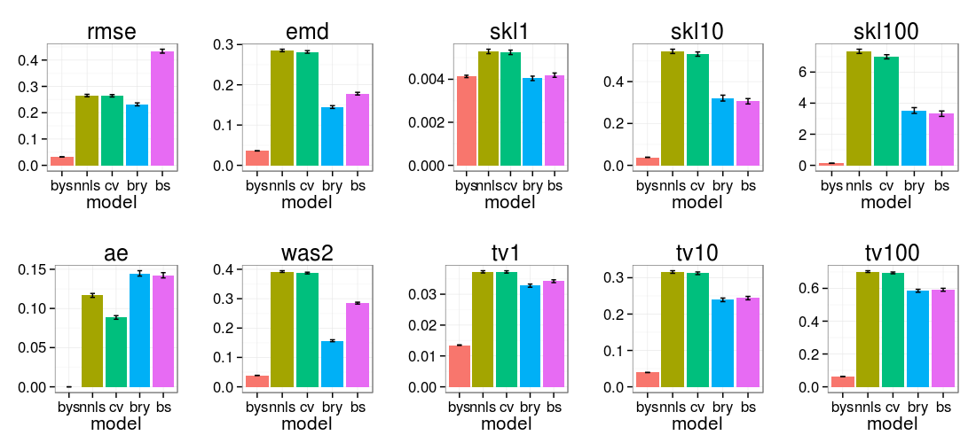
RMISE most strongly favors continuous estimates, such as the Bayes posterior mean. AE is undefined for continuous estimates and favors non-sparse estimates, such as NNLS and K-fold barycenter. On the opposite side of the spectrum, EMD favors sparse estimates, such as best-2-subset and the posterior barycenter. TV and SKL do not clearly favor sparse or non-sparse models. TV and SKL rank the models similarly regardless of the smoothing parameter used, but the smoothing parameter does influence the contrast between different methods. In the case of oversmoothing, all models have close to the minimum inaccuracy, as can be seen in the inaccuracies calculated using $TV_{1}$ and $SKL_{1}$. In the case of undersmoothing, all models have close to the maximum inaccuracy, as seen in the inaccuracies calcuated using $TV_{100}$ and $SKL_{100}$. In the case of $TV$, we see that the ratio $\max\text{err}/\min\text{err}$ is equal to 1.3 for $TV_{1}$, 1.3 for $TV_{10}$, and 1.2 for $TV_{100}$. In comparison, the ratio $\max\text{err}/\min\text{err}$ is equal to 1.9 for EMD.

The K-fold barycenter outperforms NNLS in all measures considered here: a somewhat surprising result, given that the K-fold barycenter was solely motivated by the goal of minimizing the inaccuracy as measured by EMD.

In a similar simulated experiment with $k=2$ fiber directions, uniform random weight $w_{1}$ and $w_{2}=1-w_{1}$, $\sigma^{2}=0.04$ and varying $\kappa$, we compare the correlations between errors $\text{err}=d(f,\hat{f}^{1})$ and replicate errors $RE=d(\hat{f}^{1},\hat{f}^{2})$. We find that the correlation between the EMD-based error and EMD-based replicate error, $\text{Corr}(\text{err}_{EMD},RE_{EMD})$ is above 0.4 for a range of parameter values $\kappa$ from 0.1 to 2–higher than the minimum correlations for other distances. Figure 5 contains correlations, as computed from 10000 simulations, for several values of $\kappa$.

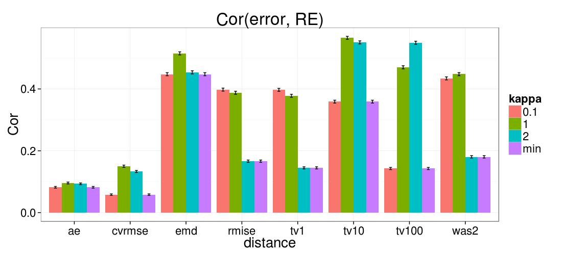
Given the practical utility of RRMSE, it is surprising to see its low correlation with the true RMISE regardless of $\kappa$. Although RRMSE is a close-to-unbiased estimated of the $\text{err}_{RMISE}$, this may come at a cost of greater variability. In contrast, $RE_{RMISE}$ has a much higher correlation with $\text{err}_{RMSE}$. At first glance $RE_{RMISE}$ appears to be a very similar procedure to $RRMSE$, but while $RRMSE$ compares the signal from replicate 1 with the raw data of replicate 2, $RE_{RMISE}$ compares the signal from replicate 1 with the signal from replicate 2. The distance measure with the highest correlation between err and $RE$ varies depending on $\kappa$. For $\kappa=0.1$, EMD has the highest correlation, $0.45\pm 0.01$; for $\kappa=1$, $TV_{1}$ has the highest correlation: $0.55\pm 0.01$, slightly higher than EMD ($0.52\pm 0.01$), while for $\kappa=2$, $TV_{10}$ has the highest correlation: $0.55\pm 0.01$. In both $TV$ and $SKL$ we see that the choice of smoothing parameter which maximizes the correlation depends on $\kappa$. Meanwhile, the 2-Wasserstein distance, which does not use smoothing, nevertheless has poor correlation between err and $RE$ at $\kappa=2$, and is consistently dominated by EMD.

To summarize, the correlation of $\text{Corr}(\text{err}_{EMD},RE_{EMD})$ is consistently comparable to the highest correlation of any other distance. Distances with fixed smoothing kernels suffer from degraded correlation at one of the extremes of the parameter range, $\kappa=0.1$ or $\kappa=2$, while the 2-Wasserstein distance also suffers from degraded correlation at high $\kappa$ even though it does not employ smoothing; in contrast, EMD is robust across $\kappa$.

These results can seemingly be explained by the fact that EMD has a combination of scale equivariance and robustness to outliers as defined in section  2.2. Even though the two properties were only defined in the Euclidean setting, they can be extended in a ‘local’ sense to any manifold via the fact that manifolds resemble Euclidean space in a small neighborhood of any point. In the particular application of DWI fiber deconvolution, the consequence of scale equivariance is that the increased error due to increased noise level will be reflected both in the error and the replicate error. Interestingly, though, we found correlations between error and replicate error in the simulation even when holding the noise level fixed. This can be explained by the fact that even if the noise level is held fixed, changes in the parameter $\kappa$ or the fiber configuration can mimic the effect of increased noise. Thus, the fact that smoothed TV and smoothed SKL are not scale equivariant explains their inconsistent performance across $\kappa$. Meanwhile, the poor performance of 2-Wasserstein distance for $\kappa=2$ can be explained by the poor robustness of 2-Wasserstein distance to outliers. When $\kappa$ is low, relative to the sample size (number of measurement directions), the NNLS algorithm finds very few ‘spurious’ directions. However, when $\kappa$ is high relative to sample size, a noise spike in a single measurement direction can cause NNLS to weight an essentially arbitrary direction in a direction orthogonal to the direction of the noise spike. This leads to the production of ‘outliers’ for high $\kappa$, which inflate the variance of the relative error as measured by 2-Wasserstein distance. On the other hand, these directional ‘artifacts’ can be removed by means of post-processing; hence it would still be interesting to revisit the application of the 2-Wasserstein distance on post-processed NNLS estimates.

DWI data was acquired in a healthy human participant in a 3T MRI instrument, at the Stanford Center for Neurobiological and Cognitive Imaging. Data was acquired at 2x2x2 $mm^{3}$ with a b-value of 2000 s/$mm^{2}$. The data consists of two sets of replicate measurements⁶⁶ 6 The data is available to download at: http://purl.stanford.edu/ng782rw8378. We identified regions of interest for analysis in the corpus callosum (CC), a region of the brain known to contain only one major fascicle, connecting the two cerebral hemispheres, and in the centrum semiovale (CSO), a part of the brain in which multiple fascicles cross. We compute K-fold replicate error ($K=10$), and replicate error of the fODF estimates. We also compute CVRMSE as a direct estimate of accuracy (with regard to RMISE). A value of $\kappa=2.2$ was estimated using cross-validation on a separate subset of the data.

CVRMSE appears to vary more smoothly across both regions of interest in the white matter. On the other hand, measures of replicate error (both RE and K-RE) show more coherent spatial variation. Both CVRMSE and replicate error are sensitive both to the configuration of the fibers in the measurement voxel and to the noise in the measurement, but their sensitivities to these factors differ. While CVRMSE is primarily sensitive to noise, EMD-based replicate error is more sensitive to the configuration of the underlying tissue (i.e. single fiber population, or more populations of fibers). The spatial variations in EMD across the corpus callosum ROI represent, therefore, variations in the degree to which different parts of the measurement contain partial volumes of other neighboring parts of the tissue. These other parts may contain either cerebrospinal fluid (the fluid the surrounds and pervades the brain), or fibers oriented in other directions than the corpus callosum fibers. The measurement noise, on the other hand, is dominated by physiological factors, and instrumental factors that vary very little across space. Hence, the relative smoothness of the variation of CVRMSE across these regions.

References

[1] Le Bihan D, Mangin JF, Poupon C, Clark CA, Pappata S, Molko N, Chabriat H. (2001). Diffusion tensor imaging: concepts and applications. Journal of magnetic resonance imaging, 13(4), 534-546.
[2] Tournier J-D, Calamante F, Connelly A (2007). Robust determination of the fibre orientation distribution in diffusion MRI: non-negativity constrained super-resolved spherical deconvolution. Neuroimage 35:1459–72
[3] Tournier, J.-D., Yeh, C.-H., Calamante, F., Cho, K.-H., Connelly, A., and Lin, C.-P. (2008). Resolving crossing fibres using constrained spherical deconvolution: validation using diffusion-weighted imaging phantom data. NeuroImage, 42: 617–25.
[4] Basser PJ. Quantifying errors in fiber-tract direction and diffusion tensor field maps resulting from MR noise. Proc. Int. Soc. Magn. Reson. Med. 1997
[5] Aganj I, Lenglet C, Jahanshad N, Yacoub E, Harel N, Thompson PM, Sapiro G. (2011). A Hough transform global probabilistic approach to multiple-subject diffusion MRI tractography. Medical image analysis, 15(4), 414-425.
[6] Frank L. Anisotropy in high angular resolution diffusion-weighted MRI. Magnetic Resonance in Medicine Volume 45, Issue 6, pages 935–939, June 2001
[7] Dell’Acqua F, Rizzo G, Scifo P, Clarke RA, Scotti G, Fazio F (2007). A model-based deconvolution approach to solve fiber crossing in diffusion-weighted MR imaging. IEEE Trans Biomed Eng 54:462–72
[8] Behrens TEJ, Berg HJ, Jbabdi S, Rushworth MFS, and Woolrich MW (2007). Probabilistic diffusion tractography with multiple fiber orientations: What can we gain? NeuroImage (34):144-45.
[9] Gudbjartsson, H., and Patz, S. (1995). The Rician distribution of noisy MR data. Magn Reson Med. 34: 910–914.
[10] Parzen E. On the estimation of a probability density fuction and mode. The Annals of Mathematical Statistics. 33(3): 1065-1076, 1962.
[11] Rubner, Y., Tomasi, C. Guibas, L.J. (2000). The earth mover’s distance as a metric for image retrieval. Intl J. Computer Vision, 40(2), 99-121.
[12] Rokem A, Yeatman J, Pestilli F, Kay K, Mezer A, van der Welt S, Wandell B. (2013). Evaluating the accuracy of models of diffusion MRI in white matter. Submitted.
[13] Efron B. Bayesian inference and the parametric bootstrap. The Annals of Applied Statistics 6 (2012), no. 4, 1971–1997.
[14] Cuturi M, Doucet A. Fast computation of Wasserstein barycenters. JMLR W&CP 32 (1) : 685–693, 2014