Thermally driven classical Heisenberg chain with a spatially varying magnetic field: Thermal rectification and Negative differential thermal resistance

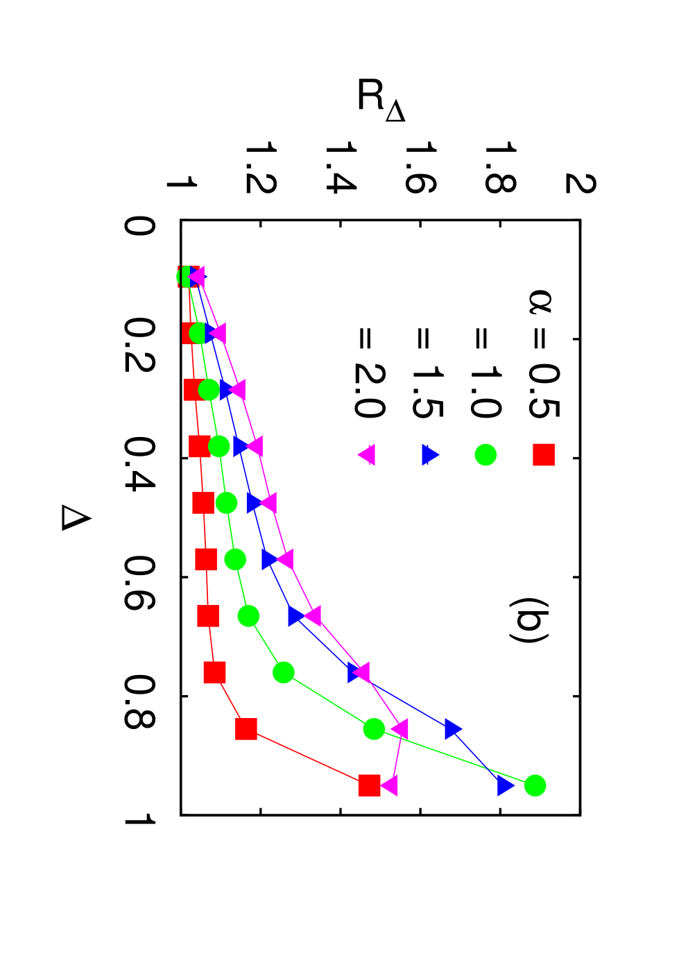
The temperature of the two thermal baths are set as $T_{l}=T(1+\Delta)$ and $T_{r}=T(1-\Delta)$, thus the average temperature of the system is $\frac{1}{2}(T_{l}+T_{r})=T$. The spatially varying magnetic field $\vec{h}_{i}$ is chosen as $(0,0,h^{z}_{i})$ and $h^{z}_{i}=h_{0}+\alpha~i/N$ is a linearly varying field where $1\leq i\leq N$; we set $h_{0}=1$ for all our results in this section. Starting from a random initial configuration of spins we let the system evolve using the DTOE dynamics until a steady state is reached and thereafter compute the thermal current using Eq. (4). We consider the system to be in forward bias for $\Delta>0$ and in backward bias for $\Delta<0$. The thermal current under the forward bias $J_{\Delta}$ and that in the backward bias $J_{-\Delta}$ are different in magnitude as can be seen from Fig. 1a. Note that the system is perfectly symmetric and homogeneous. The asymmetric heat conduction is completely brought about by the spatially varying magnetic field. We define the rectification ratio as $R_{\Delta}=|J_{-\Delta}/J_{\Delta}|$ which measure the of the amount of TR achieved. Thus for poor rectification $R_{\Delta}$ is close to unity and for good rectification $R_{\Delta}$ is very large (small) if $J_{-\Delta}\gg J_{\Delta}$ ($J_{-\Delta}\ll J_{\Delta}$). From Fig. 1b, as expected $R_{\Delta}$ is found to increase as $\alpha$ is increased i.e., when the magnetic field varies more sharply across the system (apart from some discrepancies for large $\Delta$). Thus heat conduction is asymmetric i.e. $J_{\Delta}\neq J_{-\Delta}$ and the system exhibits TR.

An interesting feature of TR in this system is the variation of the rectification ratio $R_{\Delta}=|J_{-\Delta}/J_{\Delta}|$ with the parameter $\alpha$. The rectification ratio does not increase indefinitely as $\alpha$ is increased but rather shows an intriguing nonmonotonic $\alpha$ dependence. For different values of the thermal bias $\Delta$ we compute $R_{\Delta}$ as a function of $\alpha$ and is shown in Fig. 2a. For $\alpha$ in the range $0<\alpha\lesssim\alpha_{0}$, we find $R_{\Delta}>1$ initially whereas for $\alpha\gtrsim\alpha_{0}$, $R_{\Delta}<1$, where $\alpha_{0}$ lies roughly in the range $3.5<\alpha<4.0$ (Fig. 2a). For small $\Delta$, $R_{\Delta}$ increases roughly linearly for $\alpha<\alpha_{0}$, then drops abruptly below $R_{\Delta}=1$ and then increases linearly towards unity again. For larger $\Delta$, $R_{\Delta}$ has an even more complicated nonmonotonic $\alpha$ dependence but jumps from $R_{\Delta}>1$ to $R_{\Delta}<1$ at the same $\alpha=\alpha_{0}$.

We look into the temperature dependence of $R_{\Delta}$ which is also very unusual. Generally rectification is found to deteriorate as the average temperature of the system is increased [1, 2, 25]. However in our case TR for higher temperature in certain range(s) of $\alpha$ is actually higher than that for lower temperature as can be seen in Fig. 2b. Also note that $\alpha_{0}$ shifts to higher $\alpha$ values as the average temperature is increased. Similar nontrivial dependence is seen when one studies the variation of $R_{\Delta}$ with the system size $N$. In some $\alpha$ regime, $R_{\Delta}$ decreases as $N$ is increased whereas in some other regime we get an anomalous size dependence as can be seen from Fig. 2c. Thus, depending on which $\alpha$ range one is in, the $T$ and $N$ dependences can be normal ($R_{\Delta}$ approaching unity as $T$ and $L$ increases) or anomalous. This seems to be due to a complicated interplay of the imposed thermal bias and the spatially varying magnetic field.

To understand this we look into the individual currents $J_{\Delta}$ and $J_{-\Delta}$. For relatively small values of the magnetic field the current $J$ is higher when it flows from a higher magnetic field region to a lower magnetic field region. This is due to the fact that the magnetic field tries to restrict the motion of the spins and thereby inhibits the flow of energy through the system. Now according to our definition, in the forward bias (Fig. 3a) the magnetic field increases as one approaches the colder bath - thus the motion of the spins nearer to the right end of the system is doubly restricted - one because of the low temperature and the other due to the higher magnetic fields. For the backward bias (Fig. 3b) however the effect of the higher magnetic field is somewhat compensated by the hotter bath and the spins are relatively more free to rotate in this case and therefore the system has a higher current. Since in the steady state the current through the system is a site independent constant (a consequence of the equation of continuity) the overall current of the system is dictated by the current carrying capacity of the weakest bond (corresponding to the most restricted spin) and therefore the current in the forward bias is lower than that in the backward bias. This explain why $|J_{-\Delta}|>J_{\Delta}$ for $\alpha<\alpha_{0}$, as can also be seen in Fig. 4a, and the rectification ratio $R_{\Delta}>1$; $R_{\Delta}$ increases in this region as $\alpha$ is increased because of increased asymmetry of the system. As the magnetic field increases the current starts to decrease since the orientational stiffness of the spins increases which restricts energy passage through the system. As the magnetic field becomes high the system goes into a magnetic field dominated regime which limits the current carrying capacity of the system - the weaker current $J_{\Delta}$ attains a saturation first while the relatively stronger $J_{-\Delta}$ still continues to decrease but eventually it too attains a saturation (Fig. 4a) (note that, in Fig. 4 the y-axis is a logarithmic scale in all the figures).

For a lower temperature the spins of the system are more orientationally stiff and thus this domination of the magnetic field commences at a lower value of $\alpha$. The current saturates at lower $\alpha$ (Fig. 4b) and this explains the decrease of $\alpha_{0}$ as the average temperature is decreased in Fig. 2b. With regards to the value of $\alpha_{0}$ there is no appreciable variation as the system size $N$ is altered as can be seen from Fig. 4c and also previously in Fig. 2c. The system of smaller size is closer to the ballistic limit and carries slightly more current than a system of larger size [30].

The system approaches a diffusive transport regime as the temperature $T$ or the size $N$ is increases [30], but in the forward bias condition the approach is obviously slower than in the forward bias. This is the reason that one obtains an improvement of rectification ($R_{\Delta}$ moves away from unity as in Fig. 2b,c) as $T$ or $N$ is increased in the $\alpha>\alpha_{0}$ regime. Also, as we shall show in the following, it is the motion of the $N$th spin that decides the value of $\alpha_{0}$ which therefore is independent of the length of the system to which it belongs. This is why $\alpha_{0}$ remains essentially unchanged as the system size $N$ is altered and changes only when the average temperature $T$ is changed.

Thus to summarize, there are two regimes corresponding to the two terms in the Hamiltonian (Eq. 1): (a) a spin-spin interaction dominated regime (or in other words, a temperature dominated regime) in the parameter range $0<\alpha<\alpha_{0}$ in which the current steadily decrease as $\alpha$ increases, and (b) a magnetic field dominated regime for $\alpha>\alpha_{0}$ in which the spins have a restricted motion and the current through the system changes very negligibly as $\alpha$ is varied. It is the complicated interplay of these two mutually opposing factors that gives rise to the interesting features that are observed in our system.

In order to validate the picture just presented we look into the microscopic dynamics of the individual spins now. Since the most restricted spin dictates the current (as discussed above) we look into the $S_{z}$ component of the $N$th spin (since the $N$th spin experiences the largest magnetic field amongst all the spins) and show its distribution $P_{N}(S_{z})$ as a function of the parameter $\alpha$ in Fig. 5a. Since $S_{z}\equiv\cos\theta$ ($\theta$ is the polar angle and the spins being of unit magnitude), $S_{z}$ lies in the range $[-1,1]$. For a spin which is completely free to orient itself in all possible directions, the distribution would be uniform in the range $[-1,1]$. However in presence of a finite temperature and an external magnetic field $P_{N}(S_{z})$ has an exponential form. Note that, as $\alpha$ increases, the slope of the distribution $\frac{d}{dS_{z}}\ln P_{N}(S_{z})$ increases which signifies that the spin motion gets more and more restricted. From the distribution we compute the average $\langle S_{z}\rangle$ and the standard deviation $\sigma=(\langle S_{z}^{2}\rangle-\langle S_{z}\rangle^{2})^{-1/2}$ for the $N$th spin. These two quantities are shown in Fig. 5b and Fig. 5c respectively. The average $\langle S_{z}\rangle$ approaches unity $\alpha$ increases for both the forward and backward bias conditions, and $\langle S_{z}\rangle_{\Delta}>\langle S_{z}\rangle_{-\Delta}$. The standard deviation $\sigma$ is an indicator of how freely a spin can rotate about the magnetic field. Thus larger the $\sigma$ is the more is the current $J$ that the spin allows to pass through. Fig. 5c shows that $\sigma$ for forward and backward bias decreases as $\alpha$ increases although not always monotonically for all parameters. (For the chosen parameters for the figure, $\sigma$ approximately fits to the form $\sigma^{-1}=m\alpha+c$, where $m$ and $c$ are constants - both $m$ and $c$ values are higher for $J_{\Delta}$ than $J_{-\Delta}$).

To obtain a numerical estimate of $\alpha_{0}$ where the rectification ratio $R_{\Delta}=|J_{-\Delta}/J_{\Delta}|$ shows a jump and the current attains saturation, we compute the ratio of the two $\sigma$ values, $r_{\sigma}=\sigma_{-\Delta}/\sigma_{\Delta}$, and study its variation as a function of $\alpha$. It is found that $r_{\sigma}$ increases steadily till some $\alpha$ value in the range $3.5<\alpha<4.0$ and thereafter it attains constancy (Fig. 5d). This is indeed where the magnetic field overpowers the thermal motion of the spins that we have encountered earlier - the individual currents attain saturation and the rectification ratio jumps from $R_{\Delta}>1$ to $R_{\Delta}<1$. In fact all the features that we have observed in Fig. 2a can be understood from the $\alpha$ variation of $r_{\sigma}$. In Fig. 6 we show $r_{\sigma}$ as a function of $\alpha$ for different values of $N,T$ and $\Delta$. We find that $\alpha_{0}$ remains the same for different system sizes $N$ and bias $\Delta$ values (Fig. 6a,c) and shifts only when the average temperature $T$ is varied (Fig. 6b). Also note that the nonmonotonic behavior of $R_{\Delta}$ that is observed for $\alpha<\alpha_{0}$ in some of the curves of Fig. 2 can be clearly seen in the plot for $r_{\sigma}$ (Fig. 6c).

Thus the physical picture that we had proposed to explain the features observed in rectification is corroborated by the results obtained from simulation. Thermal rectification, as exhibited by this system, shows several intriguing features that have not been observed or investigated in any of the previous works of rectification and can have a lot of technological implications in the fabrication of thermal devices. It will also be interesting to see if such peculiar dependences arise in other graded systems.

Next, we turn our attention to the emergence of NDTR in this system. Note that the current $J$ in a strictly non-decreasing function of $\Delta$ as has been obtained in Fig. 1. To make this system exhibit NDTR, we keep the temperature of one bath fixed and change the temperature of the other bath; we set $T_{l}=T$ and $T_{r}=T-\Delta$. The magnetic field is chosen to be linearly varying in space $h^{z}_{i}=h_{0}+\alpha~i/N$ as in the previous section.

The variation of the total thermal current $J$ with $\Delta$ for different values of the parameter $\alpha$ is shown in Fig. 7a. When $\alpha=0$ i.e., with an uniform magnetic field throughout the system, the current $J$ sharply increases as $\Delta$ is increased and there is no NDTR (data not shown). This is due to the absence of any mechanism to restrict the passage of energy in the bulk of the system which is required in order to observe NDTR [25].

As $\alpha$ is increased, the system exhibits NDTR for some nonzero value of $\alpha$. Thus by simply tuning the external magnetic field one obtains NDTR in this system without the need to manipulate parameters of the system. For a fixed nonzero value of $\alpha$ one can also obtain NDTR by tuning $h_{0}$ as has been shown in Fig. 7b. The physical mechanism that gives rise to NDTR is the obstruction to the flow of current by the magnetic field as has been discussed in detail in a previous work [25]. Note that when the magnetic field is increased (either by increasing $\alpha$ or $h_{0}$) further to larger values the current becomes very small and the NDTR regime disappears.

The temperature dependence of NDTR is described in Fig. 8a. It is seen that the point of emergence of NDTR $\Delta_{m}$ shifts to larger values of $\Delta$ as temperature increases. The value of the energy current increases too as the temperature is increased. From the main figure we find that the $J\sim\Delta$ curves show an excellent data collapse when the axes are rescaled as $J/T^{\nu}$ and $(\Delta-\Delta_{m})/T$; for the chosen set of parameters $\nu=2.0$ and $\Delta_{m}$ is the point where NDTR regime commences corresponding to the maximum value of current.

As has been commonly seen in previous works, NDTR becomes more pronounced as the system size $N$ is decreased. Here too, we find that the point of commencement of NDTR gradually shifts towards larger values of $\Delta$ as the system size is increased. This is depicted in Fig. 8b. The decrease of the NDTR regime due to increase in system size can however be compensated by decreasing the temperature or increasing the magnetic field suitably. We have also verified the emergence of NDTR in this system for other spatial dependence of the magnetic field. With an exponentially varying magnetic field of the form $h^{z}_{i}=h_{0}\exp(\alpha~i/N)$ we find a clear NDTR regime as $\alpha$ is increased from zero (data not shown).

References

- [1] N. Li, J. Ren, L. Wang, G. Zhang, P. Hänggi, B. Li, Rev. Mod. Phys. 84, 1045 (2012).
- [2] G. Casati, Chaos 15, 015120 (2005).
- [3] M. Terraneo, M. Peyrard, and G. Casati, Phys. Rev. Lett. 88, 094302 (2002).
- [4] B. Li, L. Wang, and G. Casati, Phys. Rev. Lett. 93, 184301 (2004).
- [5] B. Hu, D. He L. Yang and Y. Zhang, Phys. Rev. E 74, 060101(R) (2006).
- [6] B. Hu, L. Yang, and Y. Zhang, Phys. Rev. Lett. 97, 124302 (2006).
- [7] J. Lan, L. Wang, B. Li, Phys. Rev. Lett. 95, 104302 (2005).
- [8] N Yang, N Li, L Wang, and B. Li, Phys. Rev. B 76, 020301(R) (2007).
- [9] J Wang, E. Pereira and G. Casati, Phys. Rev. E 86, 010101(R) (2012).
- [10] J. Lan, B. Li, Phys. Rev. B 74, 214305 (2006).
- [11] J. Lan, B. Li, Phys. Rev. B 75, 214302 (2007).
- [12] N. A. Roberts and D. G. Walker, Int. J. Thermal Sci. 50, 648 (2011).
- [13] B. Li, L. Wang, and G. Casati, Appl. Phys. Lett. 88, 143501 (2006).
- [14] L. Wang and B. Li, Phys. Rev. Lett. 99, 177208 (2007).
- [15] D. He, S. Buyukdagli, and B. Hu, Phys. Rev. B 80, 104302 (2009).
- [16] Z.-G. Shao and L. Yang, EPL, 94, 34004 (2011).
- [17] W.-R. Zhong, P. Yang, B.-Q. Ai, Z.-G. Shao, and B. Hu, Phys. Rev. E 79, 050103(R) (2009).
- [18] W.-R. Zhong, M.-P. Zhang, B.-Q. Ai, and B. Hu, Phys. Rev. E 84, 031130 (2011).
- [19] Z.-G. Shao, L. Yang, H.-K. Chan, and B. Hu, Phys. Rev. E 79, 061119 (2009).
- [20] D. He, B.-q. Ai, H.-K. Chan, and B. Hu, Phys. Rev. E 81, 041131 (2010).
- [21] L. Wang and B. Li, Phys. Rev. Lett. 101, 267203 (2008).
- [22] C. W. Chang, D. Okawa, A. Majumdar, and A. Zettl, Science 314, 1121 (2006).
- [23] M. E. Fisher, Am. J. Phys. 32, 343 (1964).
- [24] G. S. Joyce, Phys. Rev. 155, 478 (1967).
- [25] D. Bagchi, J. Phys.: Condens. Matter 25, 496006 (2013).
- [26] L. Wang and B. Li, Phys Rev E 83, 061128 (2011).
- [27] Y. Yan, C.-Q. Wu and B. Li, Phys Rev B 79, 014207 (2009).
- [28] L. Nie, L. Yu, Z. Zheng, and C. Shu, Phys Rev E 87, 062142 (2013).
- [29] B.-q. Ai, M. An, and W.-r. Zhong, J of Chem Phys 138, 034708 (2013).
- [30] D. Bagchi and P. K. Mohanty, Phys. Rev. B 86, 214302 (2012).
- [31] H. Fröhlich and W. Heitler, Proc. Roy. Soc. (London), A155 (1936).
- [32] B. Lüthi, J. Phys. Chem. Solids 23 (1962).
- [33] R. L. Douglass, Phys. Rev. 129, 1132 (1963).
- [34] C. Hess, Eur. Phys. J. Special Topics 151, 73 (2007).
- [35] A. V. Sologubenko, T. Lorenz, H. R. Ott, and A. Freimuth, J. Low Temp. Phys. 147, 387 (2007).
- [36] A. V. Savin, G. P. Tsironis, and X. Zotos, Phys. Rev. B 72, 140402(R)(2005).
- [37] J. L. De Jongh and A.R. Miedema, Adv. Phys. 23, 1 (1974).
- [38] M. Steiner, J. Villain, and C. Windsor, Adv. Phys. 25, 87 (1976).