| 5 | Dynamical Vertex Approximation |
| Karsten Held | |
| Institute for Solid State Physics Vienna University of Technology | |
| 1040 Vienna, Austria |
1 Introduction
The theoretical description and understanding of strongly correlated systems is particularly challenging since perturbation theory in terms of the Coulomb interaction is no longer possible and standard mean field theory does not work. Also bandstructure calculations in the local density approximation (LDA) [1] which had been so successful for the calculations of many materials do not work properly as electronic correlations are only rudimentarily taken into account. A big step forward in this respect is dynamical mean field theory (DMFT) [2, 3, 4, 5] which is a mean field theory in the spatial coordinates, but fully accounts for the local correlations in time (quantum fluctuations). In comparison, standard Hartree-Fock is mean-field in space and time. DMFT is non-perturbative since all Feynman diagrams are taken into account, albeit only their local contribution for the self energy. If one is dealing with well localized - or -orbitals, these local DMFT correlations often provide the major part of the electronic correlations, which not only give rise to mass renormalizations [3, 4], metal-insulator transitions [3, 4] and magnetic ordering [6, 7], but also to unexpected new physics such as kinks [8, 9] or the filling of the Mott-Hubbard gap with increasing temperature [10]. More aspects of DMFT are discussed in other contributions to this Jülich Autumn School on DMFT at 25.
The question we would like to address here is: Can we do (or do we need to do) better than DMFT? Indeed, going beyond DMFT is necessary since many of the most fascinating and least understood physical phenomena such as quantum criticality and superconductivity originate from non-local correlations -- which are by construction beyond DMFT. And we can: A first step to include non-local correlations beyond DMFT have been cluster approaches such as the dynamical cluster approximation (DCA) [11, 12, 14] and cluster DMFT (CDMFT) [13, 12, 14]. Here, instead of considering a single site embedded in a mean-field (as in DMFT) one considers a cluster of sites in a mean-field medium. Numerical limitations however restrict the DCA and CDMFT calculations to about 100 sites. This allows for studying short-range correlations, particularly for two-dimensional lattices, but severely restricts the approach for three dimensions, for multi-orbitals, and regarding long-range correlations.
Because of that, in recent years diagrammatic extensions of DMFT were at the focus of the methodological development. An early such extension was the (: dimension) approach [15]; also the combination of the non-local spin fermion self energy with the local quantum fluctuations of DMFT has been proposed [16]. Most actively pursued are nowadays diagrammatic approaches based on the local two-particle vertex. The first such approach has been the dynamical vertex approximation (DA) [17], followed by the dual fermion approach [18], the one-particle irreducible approach (1PI) [19], and DMFT to functional renormalization group (DMF2RG) [20].
The very idea of these approaches is to extend the DMFT concept of taking all (local) Feynman diagrams for the one-particle irreducible vertex (i.e., the self energy), to the next, i.e., two-particle level. In these approaches, one calculates the local two-particle vertex; and from this non-local correlations beyond DMFT are obtained diagrammatically. Indeed, we understand most (if not all) physical phenomena either on the one-particle level (e.g. the quasiparticle renormalization and the Mott-Hubbard transition) or on the two-particle level [e.g. (para)magnons and (quantum) critical fluctuations]. Non-local correlations and associated physics on this two-particle are included in these diagrammatic extensions of DMFT, which however still include the local DMFT one-particle physics such as the formation of Hubbard bands and the metal-insulator transition or, more precisely, a renormalized version thereof. The concept of all these approaches is similar, but they differ in which two-particle vertex is taken and which diagrams are constructed, see Table 1. Depending on the approach, Feynman diagrams are constructed from full Green function lines or from the difference between and the local Green function [: (Matsubara) frequency; : wave vector]. The DF, 1PI and DMF2RG approach are also based on a generating functional integral.
| Method | Local two-particle vertex | Feynman diagrams |
|---|---|---|
| DF [18] | one-particle reducible vertex, here∗ | 2nd order, ladder |
| parquet | ||
| 1PI [19] | one-particle irreducible vertex | ladder |
| DMF2RG [20] | one-particle irreducible vertex | RG flow |
| ladder DA [17] | two-particle irreducible vertex in channel | ladder |
| full DA [17] | two-particle fully irreducible vertex | parquet |
∗ Note that at the two-particle level every two-particle vertex is one-particle irreducible; three or higher order vertices can be however one-particle reducible which has consequences for the diagrammatics if truncated at the two-particle level, see [19].
In these lecture notes, we will concentrate on DA in the following. Section 2.1 recapitulates the concept of reducible and irreducible diagrams, the parquet and Bethe Salpter equation. On this basis, we introduce in Section 2.2 the DA approach. In Section 3 we have chosen two exemplary highlights that demonstrate what can be calculated by DA and related approaches. These are: the calculation of the critical exponents for the three dimensional Hubbard model (Section 3.1) and the effect of long-range correlations on the Mott-Hubbard transition for the two dimensional Hubbard model (Section 3.2), at zero temperature antiferromagnetic fluctuations always open a gap at any interaction .
2 Feynman diagrammatics
2.1 Parquet equations
The very idea of DA is a resummation of Feynman diagrams, not in orders of the interaction as in perturbation theory but in terms of the locality of diagrams. In this sense, DMFT is the first, one-particle level since it approximates the one-particle fully irreducible vertex, i.e., the self energy , to be local, see Table 2.
| DMFT: local self energy | |
|---|---|
| DA: local fully irreducible two-particle vertex | |
| non-local self energy/correlations | |
| exact solution |
For a better understanding of reducibility and irreducibility as well as of DA later on, let us recall that in quantum field theory we calculate the interacting Green function by drawing all topologically distinct Feynman diagrams that consist of interactions and that are connected by non-interacting Green function lines , keeping one incoming and one outgoing line, see Fig. 1. Each line contributes a factor [where denotes the (Matsubara) frequency, the chemical potential and the energy-momentum dispersion relation of the non-interacting problem] and each interaction (wiggled line) contributes a factor 11 1 For a -dependent, i.e. non-local interaction the factor would be -dependent. . Here and in the following, we assume a one band model for the sake of simplicity. For an introduction to Feynman diagrams, more details and how to evaluate Feynman diagrams including the proper prefactor, we refer the reader to textbooks of quantum field theory such as [21]; a more detailed presentation including DA can also be found in [22].

Dyson equation and self energy
Instead of focusing on the Green function, we can consider a more compact object, the self energy , which is related to through the Dyson equation, see Fig. 2. The Dyson equation can be resolved for the interacting Green function:
| (1) |
Since the geometric series of the the Dyson equation generates a series of Feynman diagrams, we can only include a reduced subset of Feynman diagrams when evaluating the self energy. One obvious point is that the two outer “legs” (incoming and outgoing lines) are explicitly added when going from the self energy to the Green function, see Fig. 2. Hence we have to “amputate” (omit) these outer “legs” for self energy diagrams. More importantly, the self energy can only include one-particle irreducible diagrams. Here, one-particle (ir)reducible means that by cutting one Green function line one can(not) separate the diagram into two parts. This is since, otherwise, we would generate Feynman diagrams twice: Any one-particle reducible diagram can be constructed from two (or more) irreducible building blocks connected by one (or more) single lines. This is exactly what the Dyson equation does, see Fig. 2. For example, in the last line, we have three irreducible self energy blocks connected by two single lines. This shows that, by construction, the self energy has to include all one-particle irreducible Feynman diagrams and no one-particle reducible diagram. Since the self energy has one (amputated) incoming leg, it is a one particle vertex. It is also one-particle irreducible as explained above. Hence, the self energy is the one-particle irreducible one-particle vertex. In Fig.3 we show some diagrams that are part of the self energy, i.e., cutting one-line does not separate the diagram into two parts, and some diagrams that are not.


Two-particle irreducibility
Let us now turn to the next, the two-particle level. As illustrated in Fig. 4, the Feynman diagrams for the susceptibility (or similarly for the two particle Green function) [21] consist of (i) an unconnected part (two lines, as in the non-interacting case) and (ii) all connected Feynman diagrams (coined vertex corrections). Mathematically this yields (: inverse temperature; : spin):
| (2) | |||||
Here denotes the full, reducible vertex. In the following let us introduce a short-hand notation for the sake of simplicity, where represents a momentum-frequency-spin coordinate , , , . In this notation we have
| (3) |
as visualized in Fig. 4. Since the Green function is diagonal in spin, momentum and frequency, i.e., , some indices are the same which yields Eq. (2).
Let us now again introduce the concept of irreducibility, this time for the two-particle vertex. In this case, we consider two-particle irreducibility.22 2 Note, that one-particle irreducibility is somehow trivial since one can show that there are no one-particle irreducible diagrams for the two-particle vertex (in terms of the interacting /skeleton diagrams). In analogy to the self energy, we define the fully irreducible vertex , defined as the set of all Feynman diagrams that do not split into two parts by cutting two lines. Let us remark that here and in the following, we construct the Feynman diagrams in terms of instead of . This means that we have to exclude all diagrams which contain a structure as generated by the Dyson equation in Fig. 2 since otherwise these diagrams would be counted twice. This reduced set of diagrams with instead of is called skeleton diagrams, see [21].

The reducible diagrams of can be further classified according to how the Feynman diagram separates when cutting two internal Green functions. Since has four (“amputated”) legs to the outside, there are actually three possibilities to split into two parts by cutting two lines. That is, an external leg, say 1, stays connected with one out of the three remaining external legs but is disconnected from the other two, see Fig. 5 for an illustration. One can show by hands of the diagrammatic topology, that each diagram is either fully irreducible or reducible in exactly one channel, so that
| (4) |

∗:Note, this is only possible for one hatched side, since otherwise the same diagram might be counted twice.
Bethe-Salpeter equation
We have defined the reducible diagrams in channel as a subset of Feynman diagrams for . The rest, i.e., , is called the vertex irreducible in so that
| (5) |
In analogy to the Dyson equation, Fig. 2, the reducible vertices in turn can be constructed from . One can be connected by two s with another (which makes this diagram two-particle reducible in the channel ). This can be connected again by two s with a third etc. (allowing us to cut the two ’s at two or more different positions). This gives rise to a geometric ladder series, the so-called Bethe-Salpeter equation, see Fig. 6. Mathematically, these Bethe-Salpeter equations read in the three channels (with Einstein’s summation convention):
| (6) | |||||
| (7) | |||||
| (8) |

Parquet equations
Since an irreducible diagram in a channel is either fully irreducible () or reducible in one of the two other channels (), we can express as [this also follows directly from Eqs. (4) and (5)]:
| (9) |
We can use this Eq. (9) to substitute the last ’s in Eq. (6) (or the box in Fig. 6) by and ’s. Bringing the first on the left hand side, then yields:
| (10) | |||||
and two corresponding equations for the other two channels. The corresponding Feynman diagrams are shown in Fig. 7. If the fully irreducible vertex is known, these three equations together with Eq. (4) allow us to calculate the four unknown vertex functions and , see Fig. 7. This set of equations is called the parquet equations.33 3 Sometimes, also only Eq. (5) is called parquet equation and the equations of type Eq. (10) remain under the name Bethe-Salpeter equations. The solution can be done numerically by iterating these four parquet equations. Reflecting how we arrived at the parquet equations, the reader will realize that the parquet equations are nothing but a classification of Feynman diagrams into fully irreducible diagrams and diagrams reducible in the three channels .

The thoughtful reader will have also noticed that the interacting Green function enters in Eq. (10). This can be calculated by one additional layer of self consistency. If the reducible vertex is known, the self energy follows from the Heisenberg Eq. of motion (also called Schwinger-Dyson Eq. in this context). This is illustrated in Fig. 8 and mathematically reads:
| (11) |
That is the numerical solution of the four parquet equations has to be be supplemented by the Schwinger-Dyson Eq. (11) and the Dyson Eq. (1), so that also and are calculated self-consistently.

Let us also note that these general equations while having a simple structure in the notion can be further reduced for practical calculations: The Green functions are diagonal , there is a severe restriction in spin, there is SU(2) symmetry and one can decouple the equations into charge(spin) channels . A detailed discussion hereof is beyond the scope of these lecture notes. For more details on the parquet equations see [23], for a derivation of the equation of motion also see [24].
2.2 Dynamical vertex approximation (DA)
Hitherto, everything has been exact. If we know the exact fully irreducible vertex , we can calculate through the parquet equations Fig. 7 [Eqs. (5) and (10)] the full vertex ; from this through the Schwinger-Dyson equation of motion (11) the self energy and through the Dyson Eq. (1) the Green function . With a new we can (at fixed) recalculate etc. until convergence. Likewise if we know the exact irreducible vertex in one channel , we can calculate through the corresponding Bethe-Salpeter Eq. (6-8) and from this (self consistently) and .
But (or ) still consists of an infinite set of Feynman diagrams which we usually do not know. Since the parquet (or Bethe-Salpeter) equations generate many additional diagrams, there are however much less (albeit still infinitely many) diagrams for (or ) than for . In the case of , the bare interaction is included but the next term is already a diagram of fourth (!) order in (the so-called envelope diagram), see Fig. 9. There are no two-particle fully irreducible diagrams of second or third order in .
One approach is hence to approximate by the bare interaction only, i.e., the first two terms in Fig. 9. This is the so-called parquet approximation [23]. For strongly correlated electrons this will be not enough. A deficiency is, for example, that the parquet approximation does not yield Hubbard bands.

In DA, we hence take instead all Feynman diagrams for but restrict ourselves to their local contribution, . This approach is non-perturbative in the local interaction . It is putting the DMFT concept of locality to the next, i.e., to the two-particle level. We can extend this concept to the -particle fully irreducible vertex, so that by increasing systematically more and more Feynman diagrammatic contributions are generated; and for the exact solution is recovered, see Table 2 above.
In practice, one has to truncate this scheme at some , hitherto at the two-particle vertex level (). The local fully irreducible two-particle vertex can be calculated by solving an Anderson impurity model which has the same local and the same Green function . This is because such an Anderson impurity model yields exactly the same (local) Feynman diagrams . It is important to note that the locality for is much better fulfilled than that for . Even in two dimensions, is essentially -independent, i.e., local. This has been demonstrated by numerical calculations for the two-band Hubbard model, see [25]. In contrast, for the same set of parameters is strongly -dependent, i.e., non-local. Also and are much less local than , see [25]. There might be parameter regions in two dimensions or one-dimensional models where also exhibits a sizable non-local contributions. One should keep in mind that DA at the level is still an approximation. This approximation includes however not only DMFT but on top of that also non-local correlations on all length scales so that important physical phenomena can be described; and even in two dimensions substituting by its local contribution is a good approximation, better than replacing by its local contribution as in DMFT.
When solving the Anderson impurity model numerically, one does not obtain directly but first the local susceptibilities (or the two-particle Green function). Going from here to is possible as follows: From and , we obtain the local reducible vertex [via the local version of Eq. (2)], from this in turn we get [via inverting the local version of the Bethe-Salpeter Eqs. (6-8)], [via the local version of Eq. (5)], and finally [via the local version of Eq. (4)].
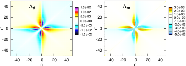
Fig. 10 shows the reducible vertex , the irreducible vertex in the particle-hole channel and the fully irreducible vertex for the three-dimensional Hubbard model on a simple cubic lattice. For more details on the calculation of , see [26] and [22]. Also note that diverges at an interaction strength below the Mott-Hubbard metal-insulator transition, which signals the breakdown of perturbation theory [27].


2.2.1 Self consistency
After calculating , we can calculate the full vertex through the parquet equations, Fig. 7; and through the Schwinger-Dyson equation, Fig. 8, the non-local self energy and Green function , as discussed in Section 2.1. Hitherto, all DA calculations have stopped at this point. That is, and are determined self-consistently but is not recalculated.
However, in principle, one can self-consistency iterate the approach. From the new we can calculate a new . From this and we obtain a new vertex etc. until convergence, see Fig. 11. This self-consistency cycle is similar as that of the DMFT but now includes self-consistency on the two-particle () level.
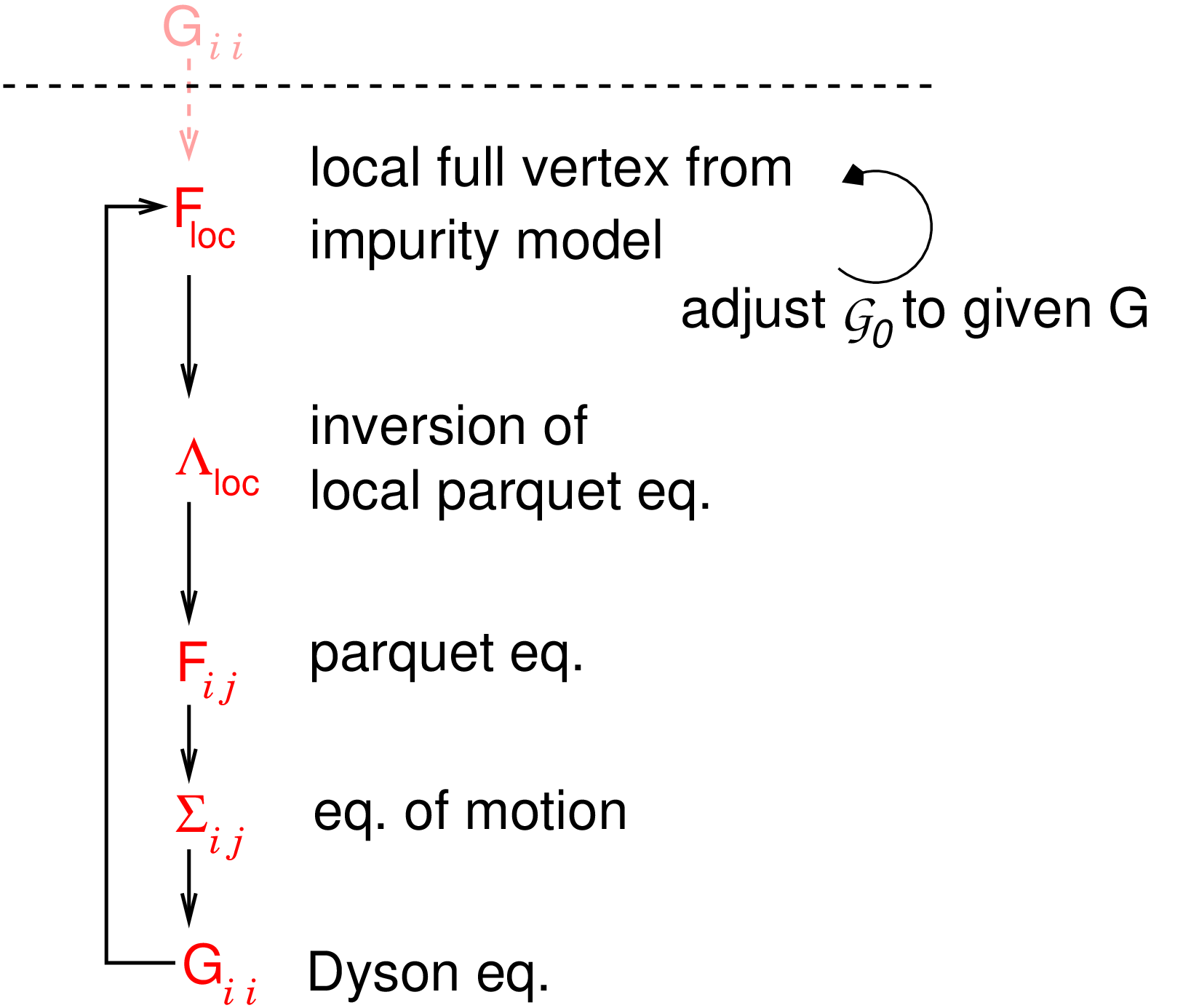
Please note that the Anderson impurity model has now to be calculated with the interacting from DA which is different from the of DMFT. As numerical approaches solve the Anderson impurity model for a given non-interacting Green function , we need to adjust this until the Anderson impurity model’s Green function agrees with the DA . This is possible by iterating as follows:
| (12) |
until convergence. Here, and denote the non-interacting and interacting Green function of the Anderson impurity model from the previous iteration. This -adjustment is indicated in Fig. 11 by the secondary cycle.

Fig. 12 compares the DA self energies calculated this way, i.e., the DA full parquet solution, with DMFT and the exact solution. The results are for a simple one-dimensional Hubbard model with nearest neighbor hopping, six sites and periodic boundary conditions so that the exact solution is still possible by an exact diagonalization of the Hamiltonian. This can be considered as a simple model for a benzene molecule. The DA results have been obtained in a “one-shot” calculation with the DMFT as a starting point. The good agreement between DA and the exact solution shows that DA can be employed for quantum chemistry calculations of correlations in molecules, at least if there is a gap [HOMO-LUMO gap between the highest occupied molecular orbital (HOMO) and the lowest unoccupied molecular orbital (LUMO)]. For molecules with degenerate ground states (i.e., a peak in the spectral function at the Fermi level), the agreement is somewhat less impressive; note that one dimension is the worst possible case for DA.
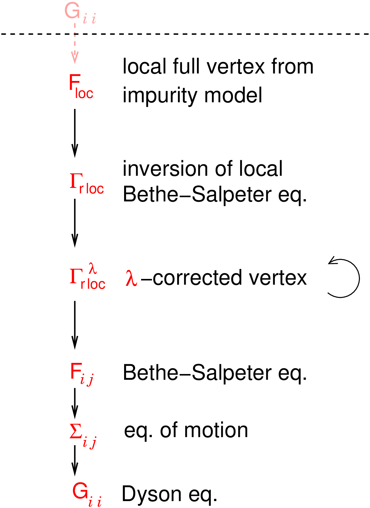
In Fig. 12, the first parquet DA results have been shown. However, most DA calculations hitherto employed a simplified scheme based on ladder diagrams, see Fig. 13. These calculations neglect one of the three channels in the parquet equations: the particle-particle channel. Both the particle-hole () and the transversal particle-hole channel () are taken into account. These channels decouple for the spin and charge vertex and can hence be calculated by solving the simpler Bethe-Salpeter equations instead of the full parquet equations. If one neglects non-local contributions in one of the channels, it is better to restrict oneself to non-self consistent calculations since part of the neglected diagrams cancel with diagrams generated by the self consistency. Instead one better does a “one shot” calculation mimicking the self-consistency by a so-called correction, see [29] for details. Physically, neglecting the particle-particle channel is justified if non-local fluctuations of particle-particle type are not relevant. Whether this is the case or not depends on the model and parameter range studied. Such particle-particle fluctuations are e.g. relevant in the vicinity of superconducting instabilities, where they need to be considered. In the vicinity of antiferromagnetic order on the other hand, the two particle-hole channels are the relevant ones (and only their magnetic spin combination). These describe antiferromagnetic fluctuations, coined paramagnons in the paramagnetic phase above the antiferromagnetic transition temperature. The DA results in the next section are for the half-filled Hubbard model. Here we are not only away from any superconducting instability, but at half-filling the interaction also suppresses particle-particle fluctuations. Hence, for the results presented below using the ladder instead of the full parquet approximation is most reasonable.
3 Two highlights
3.1 Critical exponents of the Hubbard model
The Hubbard model is the prototypical model for strong electronic correlations. At half filling it shows an antiferromagnetic ordering at low enough temperatures – for all interaction strengths if the lattice has perfect nesting. Fig. 14 shows the phase diagram of the half-filled three-dimensional Hubbard model (all energies are in units of , which has the same standard deviation as a Bethe lattice with half bandwidth ). At weak interaction strength, we have a Slater antiferromagnet which can be described by Hartree-Fock theory yielding an exponential increase of the Néel temperature with . At strong interactions, we have preformed spins with a Heisenberg interaction yielding a Heisenberg antiferromagnet with . In-between these limits, is maximal.

All of this can be described by DMFT. However, since DMFT is mean-field w.r.t. the spatial dimensions, it overestimates . This can be overcome by including non-local correlations, i.e., spatial (here antiferromagnetic) fluctuations. These reduce . In this respect, there is a good agreement between DA, DCA and lattice QMC, see Fig. 14. The biggest deviations are observed for the smaller interaction strength. In principle, these differences might originate from the fact that the DA calculations are not yet self-consistent and only use the Bethe-Salpeter Eqs. (6,7) in the two particle-hole channels instead of the full parquet equations (5,10). On the other side, however, we observe that long-range correlations are particularly important at weak coupling, cf. Section 3.2. Such long-ranged correlations cannot be captured by the cluster extensions of DMFT or lattice QMC since these are restricted to maximally sites in all three directions. More recent and accurate DDMC calculations on larger clusters [36] indeed show a smaller and, in contrast to DCA and lattice QMC better agree with DA, see Fig. 14.

Even more important are long-range correlations in the immediate vicinity of the phase transition and for calculating the critical exponents. Each finite cluster will eventually show a mean-field exponent. In this respect, we could calculate for the first time the critical exponents of the Hubbard model [31]. In Fig. 15 we show the antiferromagnetic spin susceptibility which shows a mean-field-like behavior at high temperature (and in DMFT). In the vicinity of the phase transition however, long-range correlations become important and yield another critical exponent which agrees with that of the three dimensional Heisenberg model [32] (as is to be expected from universality). In contrast for the Falikov-Kimball model, the critical exponents calculated by the related dual Fermion approach [37] agree with those of the Ising model.
Except for the immediate vicinity of the phase transition DMFT is nonetheless yielding a reliable description of the paramagnetic phase. At least this is true for one-particle quantities such as the self energy and spectral function, while the susceptibility [31] and entropy [35] show deviations in a larger -interval above .
3.2 Fate of the false Mott-Hubbard transition in two dimensions
As a second example, we recapitulate results for the interplay between antiferromagnetic fluctuations and the Mott-Hubbard transition in two dimensions. Even though the Hubbard model has been studied for 50 years, astonishingly little is known exactly. In one dimension it can be solved by the Bethe ansatz, and there is no Mott-Hubbard transition for the half-filled Hubbard model: For any finite interaction it is insulating. In infinite dimensions, on the other hand DMFT provides for an exact (numerical) solution. It has been one of the big achievements of DMFT to clarify the nature of the Mott-Hubbard transition which is of first order at a finite interaction strength [3, 4], see Fig. 16. From cluster extensions of DMFT it has been concluded that the Mott-Hubbard transition is actually at somewhat smaller values and the coexistence region where two solutions can be stabilized is smaller, see Fig. 16. However, again these cluster extensions are restricted to short-range correlations. In particular at low temperatures, there are strong long-range antiferromagnetic spin fluctuations which for example at and exceed 300 lattice sites [38]. The physical origin are antiferromagnetic fluctuations emerging above the antiferromagnetically ordered phase. In two dimensions this antiferromagnetic phase is restricted to due to the Memin-Wagner theorem, but antiferromagnetic fluctuations remain strong even beyond the immediate vicinity of the ordered phase (at ). These long-range antiferromagnetic spin fluctuations (paramagnons) give rise to pseudogap physics, where first only part of the Fermi surface becomes gaped but at lower temperatures the entire Fermi surface is gaped so that we have an insulating phase for any . Fig. 16 shows the development from local correlations (which only yield an insulating phase only relatively large ’s) to additional short-range correlations (which reduce the critical for the Mott-Hubbard transition) to long-range correlations (which reduce to zero).

At large , we have localized spins which can be described by a spin model or the Mott insulating phase of DMFT. At smaller we also have an insulator caused by antiferromagnetic spin fluctuations. These smoothly go over into the antiferromagnetic phase, which is of Slater-type for small . Since the correlation are exceedingly long-ranged, the nature of the low-temperature gap is the same as the Slater antiferromagnetic gap, even though there is no true antiferromagnetic order yet.
4 Conclusion and outlook
In the last years we have seen the emergence of diagrammatic extensions of DMFT. All these approaches have in common that they calculate a local vertex and construct diagrammatically non-local correlations from this vertex. In regions of the phase diagram where non-local correlations are short-range, results are similar as for cluster extensions of DMFT. However, the diagrammatic extensions also offer the opportunity to include long-range correlations on an equal footing. This allowed us to study critical phenomena and to resign the Mott-Hubbard transition in the two-dimensional Hubbard model to its fate (there is no Mott-Hubbard transition).
These were just the first steps. Indeed the diagrammatic extensions offer a new opportunity to address the hard problems of solid state physics, from superconductivity and quantum criticality to quantum phenomena in nano- and heterostructures. Besides a better physical understanding by hands of model systems, also realistic materials calculations are possible – by AbinitioDA[41]. Taking the bare Coulomb interaction and all local vertex corrections as a starting point, AbinitioDA includes DMFT, and non-local correlations beyond within a common underlying framework. Both on the model level and for realistic materials calculations, there is plenty of physics to explore.
Acknowledgments. I sincerely thank my coworkers S. Andergassen, A. Katanin, W. Metzner, T. Schäfer, G. Rohringer, C. Taranto, A. Toschi, and A. Valli for the fruitful cooperations on diagrammatic extensions of DMFT in the last years, and G. Rohringer also for reading the manuscript. This work has been financially supported in part by the European Research Council under the European Union’s Seventh Framework Programme (FP/2007-2013)/ERC through grant agreement n. 306447 (AbinitioDA) and in part by the Research Unit FOR 1346 of the Deutsche Forschungsgemeinschaft and the Austrian Science Fund (project ID I597).
References
- [1] R.O. Jones and O. Gunnarsson, Rev. Mod. Phys. 61, 689 (1989).
- [2] W. Metzner and D. Vollhardt, Phys. Rev. Lett. 62 324 (1989).
- [3] A. Georges and G. Kotliar, Phys. Rev. B 45 6479 (1992).
- [4] A. Georges, G. Kotliar, W. Krauth and M. Rozenberg, Rev. Mod. Phys. 68, 13 (1996).
- [5] G. Kotliar and D. Vollhardt, Phys. Today 57, No. 3 (March), 53 (2004).
- [6] M. Jarrell, Phys. Rev. Lett. 69 168 (1992).
- [7] K. Held and D. Vollhardt, Eur. Phys. J. B 5, 473 (1998).
- [8] K. Byczuk, M. Kollar, K. Held, Y.-F. Yang, I. A. Nekrasov, T. Pruschke and D. Vollhardt, Nature Physics 3 168 (2007); A. Toschi, M. Capone, C. Castellani, and K. Held, Phys. Rev. Lett. 102, 076402 (2009); C. Raas, P. Grete, and G. S. Uhrig, Phys. Rev. Lett. 102, 076406 (2009).
- [9] K. Held, R. Peters, A. Toschi, Phys. Rev. Lett. 110, 246402 (2013).
- [10] S.-K. Mo, H.-D. Kim, J. W. Allen, G.-H. Gweon, J. D. Denlinger, J. -H. Park, A. Sekiyama, A. Yamasaki, S. Suga, P. Metcalf, and K. Held, Phys. Rev. Lett. 93 076404 (2004).
- [11] T. Maier, M. Jarrell, T. Pruschke and M. H. Hettler, Rev. Mod. Phys. 77 1027 (2005).
- [12] A. I. Lichtenstein and M. I. Katsnelson, Phys. Rev. B 62 9283 (R) (2000).
- [13] G. Kotliar, S. Y. Savrasov, G. Pálsson and G. Biroli, Phys. Rev. Lett. 87 186401 (2001).
- [14] E Koch Quantum cluster methods in E. Pavarini, E. Koch, D. Vollhardt, and A. Lichtenstein, (Eds.): Autumn School on Correlated Electrons. DMFT at 25: Infinite Dimensions, Reihe Modeling and Simulation, Vol. 4 (Forschungszentrum Jülich, 2014).
- [15] A. Schiller and K. Ingersent, Phys. Rev. Lett. 75 113 (1995).
- [16] E. Z. Kuchinskii, I. A. Nekrasov and M. V. Sadovskii, Sov. Phys. JETP Lett. 82 98 (2005).
- [17] A. Toschi, A. A. Katanin, and K. Held, Phys. Rev. B 75, 045118 (2007); Prog. Theor. Phys. Suppl. 176, 117 (2008).
- [18] A. N. Rubtsov, M. I. Katsnelson, and A. I. Lichtenstein, Phys. Rev. B 77, 033101 (2008).
- [19] G. Rohringer, A. Toschi, H. Hafermann, K. Held, V.I. Anisimov, and A. A. Katanin, Phys. Rev. B 88, 115112 (2013).
- [20] C. Taranto, S. Andergassen, J. Bauer, K. Held, A. Katanin, W. Metzner, G. Rohringer, and A. Toschi, Phys. Rev. Lett. 112, 196402 (2014).
- [21] A. A. Abrikosov, L. P. Gorkov and I. E. Dzyaloshinski, Methods of Quantum Field Theory in Statistical Physics (Dover, New York, 1963).
- [22] G. Rohringer, Ph.D. thesis, Vienna Unversity of Technology (2013).
- [23] N. E. Bickers, “Self consistent Many-Body Theory of Condensed Matter” in Theoretical Methods for Strongly Correlated Electrons CRM Series in Mathematical Physics Part III, Springer (New York 2004).
- [24] K. Held, C. Taranto, G. Rohringer, A. Toschi, Hedin Equations, GW, GW+DMFT, and All That in E. Pavarini, E. Koch, D. Vollhardt, and A. Lichtenstein, (Eds.): The LDA+DMFT approach to strongly correlated materials - Lecture Notes of the Autumn School 2011 Hands-on LDA+DMFT, Reihe Modeling and Simulation, Vol. 1 (Forschungszentrum Jülich, 2011).
- [25] T. A. Maier, M. S. Jarrell, and D. J. Scalapino, Phys. Rev. Lett. 96, 047005 (2006).
- [26] G. Rohringer, A. Valli, and A. Toschi, Phys. Rev. B 86, 125114 (2012).
- [27] T. Schäfer, G. Rohringer, O. Gunnarsson, S. Ciuchi, G. Sangiovanni, and A. Toschi, Phys. Rev. Lett. 110, 246405 (2013).
- [28] For details on the numerical solution of the parquet equation and how to stabilize it enforcing among others the crossing symmetry, see S. X. Yang, H. Fotso, J. Liu, T. A. Maier, K. Tomko, E. F. D’Azevedo, R. T. Scalettar, T. Pruschke, and M. Jarrell, Phys. Rev. E 80, 046706 (2009); K.-M. Tam, H. Fotso, S.-X. Yang, Tae-Woo Lee, J. Moreno, J. Ramanujam, and M. Jarrell, Phys. Rev. E. 87, 013311 (2013).
- [29] A. A. Katanin, A. Toschi, and K. Held, Phys. Rev. B 80, 075104 (2009).
- [30] A. Valli, Ph.D. thesis, Vienna University of Technology (2013); A. Valli, T. Schäfer, P. Thunström, G. Rohringer, S. Andergassen, G. Sangiovanni, K. Held, and A. Toschi, arXiv:1410.4733.
- [31] G. Rohringer, A. Toschi, A. A. Katanin, and K. Held,Phys. Rev. Lett. 107, 256402 (2011).
- [32] M.F. Collins, “Magnetic Critical Scattering”, Oxford University Press, New York, 1989.
- [33] P. R. C. Kent, M. Jarrell, T. A. Maier, and Th. Pruschke, Phys. Rev. B 72, 060411 (2005).
- [34] R. Staudt, M. Dzierzawa, and A. Muramatsu, Eur. Phys. J. B 17, 411 (2000).
- [35] S. Fuchs, E. Gull, L. Pollet, E. Burovski, E. Kozik, T. Pruschke, and M. Troyer, Phys. Rev. Lett. 106, 030401 (2011).
- [36] E. Kozik, E. Burovski, V. W. Scarola, and M. Troyer, Phys. Rev. B 87,2051102 (2013).
- [37] A. E. Antipov, E. Gull, and S. Kirchner, Phys. Rev. Lett. 112, 226401 (2014).
- [38] T. Schäfer, F. Geles, D. Rost, G. Rohringer, E. Arrigoni, K. Held, N. Blümer, M. Aichhorn, and A. Toschi, arXiv:1405.7250.
- [39] N. Blümer, Ph.D. Thesis, University Augsburg (2003).
- [40] H. Park, K. Haule and G. Kotliar, Phys. Rev. Lett. 101, 186403 (2008).
- [41] A. Toschi, G. Rohringer, A. A. Katanin, K. Held, Annalen der Physik 523, 698 (2011); cf. [24]
Index
- Bethe-Salpeter equation §2.1
- cluster dynamical mean field theory (CDMFT) §1, Fig. 16
- critical exponents Fig. 15
- dual fermion (DF) approach §1
- dynamical cluster approximation (DCA) §1, Fig. 14
- dynamical mean field theory (DMFT) §1, Fig. 16
- dynamical mean field theory to functional renormalization group (DMF2RG) approach §1
- dynamical vertex approximation (DA) Document, §2.2, Fig. 16
- Dyson equation §2.1
- Feynman diagrams §2
- functional renormalization group (fRG) §1
- GW approach §4
- Hubbard model Fig. 14, Fig. 16, §3.1
- Mott-Hubbard transition §3.2
- non-local correlations §1, Fig. 14
- one-particle irreducible §2.1
- parquet equations §2.1, §2.1
- quantum Monte Carlo (QMC) Fig. 16
- self energy §2.1
- variational cluster approximation (VCA) Fig. 16
- vertex §1, §2.1, §2.2