Efficient Brownian Dynamics Simulation of Single DNA with Hydrodynamic Interactions in Linear Flows
Abstract
The coarse-grained molecular dynamics (MD) or Brownian dynamics (BD) simulation is a particle-based approach that has been applied to a wide range of biological problems that involve interactions with surrounding fluid molecules or the so-called hydrodynamic interactions (HIs). In this paper, an efficient algorithm is proposed to simulate the motion of a single DNA molecule in linear flows. The algorithm utilizes the integraing factor to cope with the effect of the linear flow of the surrounding fluid and applies the Metropolis method (MM) in [N. Bou-Rabee, A. Donev, and E. Vanden-Eijnden, Multiscale Model. Simul. 12, 781 (2014)] to achieve more efficient BD simulation. Thus our method permits much larger time step size than previous methods while still maintaining the stability of the BD simulation, which is advantageous for long-time BD simulation. Our numerical results on -DNA agree very well with both experimental data and previous simulation results. Finally, when combined with fast algorithms such as the fast multipole method which has nearly optimal complexity in the total number of beads, the resulting method is parallelizable, scalable to large systems, and stable for large time step size, thus making the long-time large-scale BD simulation within practical reach. This will be useful for the study of membranes, long-chain molecules, and a large collection of molecules in the fluids.
pacs
05.40.-a, 47.27.eb, 87.15.A-I Introduction
The dynamics of a single DNA or polymer macromolecule in fluid flow has been extensively investigated experimentally ([17, 24] and references therein), theoretically [4, 16, 3] and numerically [11, 23]. Bulk rheological experiments such as flow bi-refringence and light scattering measurements give inference of polymer conformation, orientation, and chain stretch in fluid flows. The advent of single molecule visualizations using fluorescence microscopy allows for the direct observation of complex dynamics of individual macromolecules in dilute solutions under shear, extensional, and general two-dimensional mixed flows [7, 9, 22, 24, 25]. These measurements provide data for direct comparison against fully parametrized models of macromolecules, such as the bead-spring model for DNA with finite extensibility, excluded volume (EV) [18] effects and hydrodynamic interactions (HI) [23]. Brownian dynamics (BD) simulations of bead-spring and bead-rod models with free-draining assumption (no hydrodynamic interactions) give quantitative agreement with dynamical polymer behavior from single-molecule experiments [10, 14, 26].
Following Ermak and McCammon [4], Schroeder et al. modeled the DNA macromolecule as a system of particles subject to interparticle forces, fluctuating HI and EV forces [23]. They designed a semi-implicit predictor-corrector scheme for simulating the Brownian system, and illustrated how effects of HI and EV between monomers in a flexible polymer chain influence both the equilibrium and non-equilibrium physical properties of DNA macromolecules [23], consistent with the experimental observations. The non-local HI between the DNA macromolecule and the surrounding fluid involves an integral of hydrodynamic forces between a point and the rest of the macromolecule. Within the coarse-grained framework, this integral is equivalent to a sum of all hydrodynamic forces between a bead and the rest of the system. Here we adopt the Rotne-Prager-Yamakawa (RPY) tensor [19] (i.e., the mobility tensor) for HI effects:
| (1) |
| (2) | |||
| (3) | |||
where is the mobility of bead due to bead in three dimensions, the identity matrix, and is the bead resistivity with the solvent viscosity and the radius of beads.
There are two main challenges for the long-time large-scale BD simultions with HI and EV effects. First, the correlated random noises in the change of displacement vectors at each time step are proportional to with the time step size. This makes the design of high-order marching scheme very difficult and forces very small for many explicit or semi-implicit numerical schemes in order to avoid the numerical instability. The problem becomes much more severe for long-time BD simulations since it then requires a very large total number of time steps for the system to reach the desired state, which very often leads to weeks of simulation time even for one run.
Second, the direct evaluation of the particle interaction at each time step requires operations where is the total number of particles in the system; and the generation of the correlated randome displacements requires operations if the standard Choleski factorization is used or if the Chebyshev spectral approximation is used for computing the product of the matrix square root and an arbitrary vector (here is the condition number of the covariance matrix) (see, for example, [12]).
To summarize, in order to efficiently utilize the BD simulation as a practical tool to study the properties of large systems, say, many polymers or a large collection of DNA molecules in a fluid, it is essential to address the following two questions: how to numerically integrate the system with greater accuracy and better stability property which enables much large time step size? How to expedite the calculations of long-range particle interactions and associated correlated random effects in BD simulations with HI, especially for large ?
For BD simulations near equilibrium, a Metropolis scheme for the temporal integration has been recently proposed [1, 2] for a Markov process whose generator is self-adjoint (with respect to a density function) to expedite simulations to reach equilibrium in a timely fashion. Under this scheme, stable and accurate BD simulations of DNA in a solvent are obtained using time step sizes that are orders of magnitude larger than those for predictor-corrector schemes [14, 11, 23]. However, such a Metropolis scheme relies heavily on the self-adjointness of the Markov process generator for a quiescent flow.
In this work, we present an efficient algorithm for the simulations of the dynamics of DNA macromolecules under linear flows. Our method is based upon the Metropolis scheme developed in [2] for self-adjoint diffusions, which is applicable for the study of the DNA molecule to its equilibrium configurations in a quiescent flow. When a linear flow such as an extensional or a shear flow is present in the surrounding fluid, the diffusion process is not self-adjoint anymore. We first apply the method of integrating factors to recast the associated system of stochastic differential equations (SDE) into a form such that the effect of the linear flow is taken into account by the integrating factor. We then modify the Metropolis scheme in [2] to update the displacements of beads which are the coarse-grained representation of the long chain DNA molecule. Our numerical experiments show that our scheme allows much greater time step size in the BD simulation and avoids the numerical instability. The numerical results on the study of -DNA agree very well with the expermental data [25, 24] and previous simulation results [23]. Moreover, the total simulation time is significantly reduced in our methods as compared with the semi-implicit predictor-corrector scheme [23].
When the system involves a large number of particles, as in the case of the study of lipid bilayer membranes, long chain polymers, or a large collection of DNA molecules, we observe that recent work in [12, 15] reduces the computational cost of particle interactions from to and the cost of generating the correlated random displacements from or to , which leads to an essentially linear algorithm with respect to the total number of particles in the BD simulation. The method developed in [12, 15] extends the original fast multipole method (FMM) [5] to the case of the RPY tensor and combines it with the spectral Lanczos decomposition method (SLDM) to generate corelated random vectors whose correlation is determined by the RPY tensor. We expect that long-time large-scale BD simulations (with or without linear flows) for large systems are within practical reach when our modified Metropolis scheme is combined with the method in [12, 15]. Since the experimental or simulation results for large systems do not seem to appear in the literature, we will only present some numerical results which indicate the linear scaling of methos in [12, 15] and report the results on the BD simulation of large system on a later date.
This paper is organized as follows. In section II the formulation for the BD simulation is presented along with a discussion on the relevant physical parameters and forces. Section III provides a detailed description of the numerical method used in this paper. In section IV we demonstrate the performance of our numerical scheme by comparing our numerical results with the experimental data [25, 24] and previous simulation results [23] where the motion of a single DNA molecule in a quiescent, extensional, or shear flow is studied and the DNA molecule is modeled via beads. In section V we briefly discuss the extension of our method to the study of large systems by combining it with the FMM for the RPY tensor and other fast algorithms. Finally section VI contains a short conclusion and discussion for future work.
II Brownian Dynamic Simulation of a DNA molecule with HI
The DNA or polymer macromolecule is coarse-grained into a system of beads described by the Langevin equation [4] with hydrodynamic interactions. The governing equation for the position vector of the th bead is
| (4) |
where is the mass of bead , is the solvent velocity, and is the friction coefficient tensor. The coefficient matrix connects the thermal fluctuations of the particles through hydrodynamic interactions. In the Ermak-McCammon model [4], it is related to with , where is the thermal energy. is the thermal fluctuation modeled as a Wiener process with mean and variance . Thus, the RHS of eq. 4 is the total force acting on the bead including the drag force, total inter-particle force and the thermal fluctuating HI.
Ignoring the bead inertia, eq. 4 can be written as a first-order stochastic differential equation (SDE):
| (5) | |||
where is the transpose of the constant velocity gradient tensor of the linear far-field flow velocity and ( in a quiescent flow). The random Wiener process in the SDE is related to as: where is a random vector with the standard Gaussian distribution.
is the mobility tensor of size and for the N-bead chain the tensor is related to the thermal energy through the friction coefficient tensor as . As in [4, 23], we use the RPY tensor for .
In the absence of external driving forces, the covariance between the bead displacements satisfy the following relation
| (6) |
Hence, the coefficient matrix is connected with via the formula . We remark here that the choice of is not unique and fast algorithms for generating these correlated random displacements actually take advantage of this fact. Finally, we observe that for the RPY tensor, is always zero and eq. 5 is reduced to
| (7) |
II.1 Nondimensionalization of the SDE (7)
The bead-spring chain model is widely used for BD simulations of a DNA molecule. In the bead-spring chain model, the DNA molecule is represented as a chain of beads of radius with adjacent beads connected by a spring. Each spring contains Kuhn steps of length . So the maximum length of each spring is , and the characteristic contour length of the double stranded DNA molecule is approximately as the size of each bead is much smaller than the length of each spring and thus neglected. We denote the Hookean spring constant by . The characteristic length is chosen to be and the characteristic time is chosen to be , where is the bead resistivity appeared in the RPY tensor (3). We scale the length and time by and , respectively and nondimensionalize eq. 7 into the following dimensionless form:
| (8) |
Here with a slight abuse of notation, we have used the same notation to denote all corresponding dimensionless quantities.
II.2 Choices of the Velocity Gradient Tensor
We now specify the velocity gradient tensor in eq. 8 and restrict our attention to the following two linear planar flows. The first one is the extensional flow where with the extension rate. The second is the shear flow where with the shear rate. We define the Peclet number for the extensional flow and for the shear flow, respectively. Then the dimensionless velocity gradient tensor in eq. 8 is given by the following formulas:
| (9) |
Here for the extensional flow and for the shear flow.
II.3 Specification of the Forcing Term
The force in eq. 8 contains two parts: the force exerted by the connected springs and the force due to the finite size of the beads. We adopt the Marko-Siggia’s wormlike chain (WLC) spring law [16] to model the spring force between beads. In the WLC model, the dimensionless spring force acting on the th bead by the th spring is
| (10) |
where , is the distance vector between bead and , is the length of , and is the maximum distance between these two beads. Since all interior beads are connected with two springs from two sides, the net entropic spring force acting on the th bead is
| (11) |
with . For later use, we also record the potential for the th spring below
| (12) |
For the force due to the finite size of the beads, we adopt the excluded volume force in [18, 23] given by the formula
| (13) |
where , and is the dimensionless excluded volume parameter. And the excluded volume potential between bead and bead is given by
| (14) |
Finally, the total force acting on bead is the sum of the spring forces and the excluded volume forces, that is,
| (15) |
III Numerical Algorithm for BD Simulations in Linear Flows
In the past, a semi-implicit predictor-corrector scheme [9, 23, 26] is often used for the temporal integration in BD simulations. A major problem associated with that scheme is that a very small time step size has to be used in order to avoid the numerical instability, which leads to an excessively large number of time steps and a very long total simulation time. Recently, a Metropolis integrator has been developed to integrate the self-adjoint diffusion equations [2] for BD simulations in a quiescent flow.
Here we extend the algorithm in [2] to study BD simulations in linear flows. We first introduce an integrating factor and rewrite eq. 8 as follows:
| (16) |
Similar to the algorithm in [2], we now update the position vector as follows:
1. Compute the vector as follows:
| (17) | ||||
where the functions and are defined by the following formulas:
| (18) | ||||
| (19) | ||||
2. Calculate the acceptance probability as follows:
| (20) | ||||
where , is the total potential energy, and is obtained via the formula
| (21) |
3. Generate a Bernoulli random number , that is, generate a uniformly distributed random number on and set to if and otherwise.
4. Compute the updated position vector at time by the formula
| (22) |
with the matrix or for the extensional or shear flow, respectively. Here and are given by the formulas:
| (23) |
| (24) |
In other words, the position vector will be updated only if the Bernoulli random number is equal to . This is the essence of the Metropolis algorithm for Monte-Carlo simulations.
IV Numerical Results
Common measures of the “stretch” of a DNA molecule under flow are the molecular fractional extension ( is the unit vector in the x direction)
| (25) |
and its ensemble average , where is the total number of experiments (or simulations). Here we first compare the transient fractional extensions of a -DNA between the experimental data, semi-explicit numerical simulations [23], and our Metropolis scheme simulations. The initial DNA configurations in these simulations are the equilibrium DNA configurations in the absence of flow from the Metropolis scheme.
For the purpose of comparison, we use the same values of physical and model parameters as in [23]. That is, the viscosity of solvent is () and the relaxation time is seconds. The -DNA is modeled with beads of radius connected by springs, where each spring has Kuhn steps of size and the contour length is . Finally, the excluded volume parameter .
To mimic the experimental configurations, it is essential [23, 21] to first simulate the DNA molecule to its equilibrium in a quiescent flow, i.e., in eq. 8, which is now a self-adjoint stochastic differential equation that can be efficiently solved to an equilibrium state using the Metropolis scheme in section III. At the beginning of the no-flow simulations, beads are equally spaced on the x-axis. The Metropolis scheme allows for relatively large time step (an order of magnitude larger), consequently saving a significant amount of computation time for running no-flow simulations compared to the semi-implicit predictor-corrector scheme in [23]. The flow-free simulation is continued until an equilibrium configuration is reached, which is often 10-20 relaxation times . After the equilibrium is reached for a DNA in a quiescent flow, we then turn flow on in the simulations and sum up to obtain the updated configuration and the mean fractional extension of a DNA molecule under linear flow.
 |
 |
The transient fractional extension from these simulations is summarized in Figure 1, which shows two sets of comparison for Deborah number and for panels (a) and (b), respectively. Figure 1 is simulated by using the modified Metropolis integrator scheme with an integrating factor (eq. 8 in section III, ). Thin curves are individual trajectories from experiments, filled circles are the ensemble average from experiments, filled triangles are ensemble average from Schroeder et al. [23], and our results are the empty triangles. We observe that, in both panels, our results are in good agreement with the experiment results. However, our simulations are orders of magnitude more efficient because a time-step is used for results in panels (a), and is used for panel (b). In comparison, a much smaller time step for and cases are necessary for the predictor-corrector scheme [23, 21].
 |
 |
Similar comparison of a single DNA molecule in a planar extensional flow between experiment and simulations are also conducted in [11]. Figure 2 compares our results against those from [25] for a DNA molecule in an extensional flow with , , , , for the temperature and . Figure 2(a) is for , , and . Figure 2(b) is for , , and . The thin curves are trajectories from experiments [25], filled circles are the ensemble average of experimental results, and empty circles are the ensemble average from our modified Metropolis integrator simulations. For (panel (a)) our average is almost identical to the simulation average from [11] (bottom panel of their figure 2). For (panel (b)), it is clear that our simulation results are in better agreement with experimental results than those from Jendrejack et al. [11]. In these Metropolis integrator simulations for both in panel (a) and in panel (b). Even though this time step is slightly smaller than those used in [11], our Metropolis algorithm with the integrating factor is second-order accurate [1, 2] and no matrix inversion is needed. In section V we describe how our numerical algorithm can be further improved by efficiently calculating the HI using FMM when the system size is large.
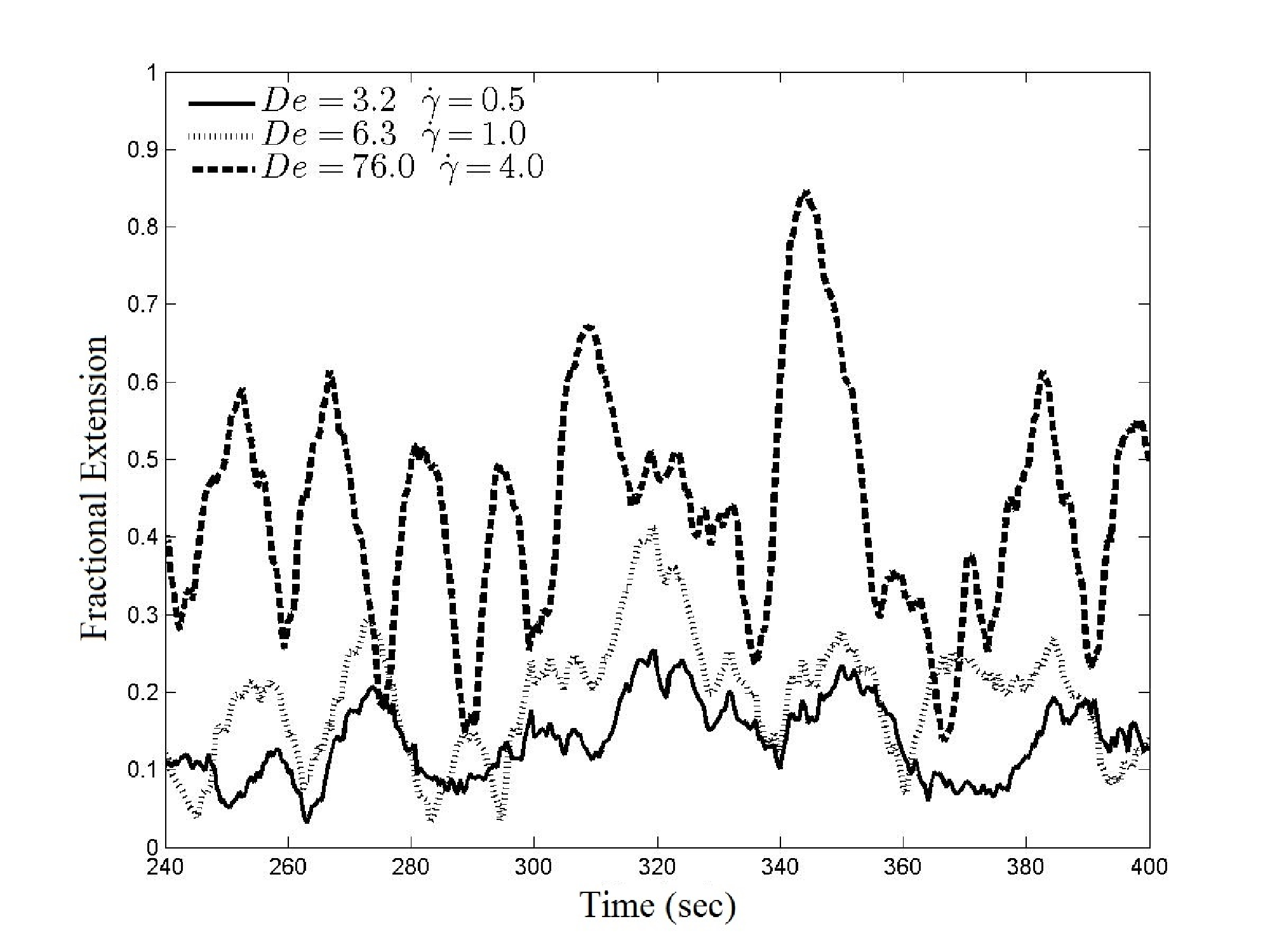
Next we compare the mean fractional extension of a DNA molecule against experiments [24] and Jendrejack et al.’s simulations [11]. The physical parameters in the experiments are [24]: bead radius , and temperature is fixed at . Two viscosities are considered in the experiments, and for the shear flow cases, while only is used for the case of extensional flow (based on the experiments in [24]). For the corresponding simulations in [11] the number of beads is , Kuhn step size , the number of springs per Kuhn step , and the contour length .

Figure 3 shows the fractional extension versus time for three cases: . As expected, larger mean extension of the DNA molecule is expected at a higher shear rate. From these results the mean fractional extension is computed by taking the averages over a long duration.
Figure 4 shows the comparison of mean fractional extension between experiments [24], Jendrejack et al.’s simulations [11] and our simulations. Experimental data are shown in filled dark disks for the extensional flow and dark circles for the shear flow, and the thin solid curves are their best fits. Simulation results from [11] are thick dashed (with HI) and dash-dotted (without HI, or free-draining (FD)) curves. Our simulation results are shown using the red symbols in the legends, and their best fits are the thin dashed curves. It is clear that our results agree well with experimental data for the shear flow cases. For the extensional flow cases, our results agree better with simulation results from [11] for all values of De. At larger De (De ), all three agree well for the extensional flow cases.
V Extension to Large Systems
In the numerical algorithm described in section III, the RPY tensor is constructed explicitly, the matrix vector product is computed directly, the uppertriangular matrix is obtained by the Cholesky decomposition with its determinant simply the product of its diagonal entries. This is affordable for the numerical experiments presented in section IV since the number of beads is only . However, for large systems, say, , the computational cost of these standard direct algorithms becomes prohibitively expensive since the matrix vector product requires operations, the Cholesky factorization requires operations, and each BD simulation often requires more than time steps. Thus, fast algorithms become a necessity in order to make long-time large-scale BD simulations practical.
As mentioned in section I, recently a fast multipole method for the RPY tensor (RPYFMM) has been developed in [15]. The fundamental observation in [15] is that the RPY tensor can be decomposed as follows:
| (26) | |||||
where .
With this decomposition, the matrix vector product for a given vector can be interpreted as a linear combination of four harmonic sums with suitably chosen source charges and dipoles. In other words, the matrix vector product can be evaluated by four calls of the classical FMM for Coulomb interactions in three dimensions [6]. Thus, the RPYFMM avoids the explicit construction of the RPY tensor and reduces the computational cost of to in both CPU time and memory storage.
We observe further that the Cholesky factor of the RPY tensor can be replaced by any matrix which satisfies the same matrix equation (note that there are actually infinitely many matrices satisfying this matrix equation, see, for example, [12] for details). Indeed, [15] also proposed to replace the Cholesky factor by and compute by combining the classical Spectral Lanczos Decomposition Method (SLDM) with the RPYFMM. The resulting algorithm has complexity with the condition number of the RPY tensor . We remark here that for most BD simulations with HIs, the beads do not overlap with each other due to the EV force and our numerical experiments show that the condition number of the RPY tensor in this case is fairly low. This indicates that the RPYFMM-SLDM method is essentially a linear algorithm for computing . The timing results presented in Table 1 and Table 2 clearly demonstrate of linear scaling of the RPYFMM and RPYFMM-SLDM methods.
| N | |||
|---|---|---|---|
| 1,000 | 0.20897 | 0.31495 | 1.6008e-02 |
| 10,000 | 1.6058 | 30.6643 | 5.5339e-02 |
| 100,000 | 16.172 | 2738.48 | 8.3803e-02 |
| 1,000,000 | 160.24 | 271009.4 | 1.1603e-01 |
| N | m | ||
|---|---|---|---|
| 1,000 | 4 | 0.54192 | 6.21032e-06 |
| 10,000 | 4 | 9.03360 | 6.24604e-04 |
| 100,000 | 6 | 111.80 | 7.92857e-04 |
| 1,000,000 | 12 | 2180.8 | 2.91239e-04 |
Finally, we would like to remark here that recent developments in the fast multipole methods and fast direct solvers also enable a linear algorithm for computing the determinant of a matrix with certain hierachical low rank structure [8, 13, 20]. By incorporating all these fast algorithms into our current numerical scheme, we obtain a numerical algorithm which is stable even for relatively large time step size and scales linearly with respect to the number of particals (or beads) in the system.
VI Conclusion and Discussion
We have extended the Metropolis integrator in [2] to study BD simulations with HIs in linear flows. The method utilizes the integraing factor to absorb the effect of the linear flow and permits much larger time step sizes for BD simulations with HIs in linear flows. We have applied our method to study the fractional stretch and the mean stretch of a single -DNA molecule in planar linear flows. Our numerical results agree very well with experimental data [25, 24] and other simulation results [23] in the literature.
We have also discussed the extension of our method to large systems in section V. By incorporating the RPYFMM and other fast algorithms into the scheme, the resulting algorithm admits large time step sizes and has nearly optimal complexity (i.e., or ) in the number of particles in the system. Thus, even though many of these fast algorithms have a large prefactor (say, ) in front of , the combination of our fast algorithm with modern computers makes long-time large-scale BD simulations with HIs within practical reach. We are currently incorporating these fast algorithms into the modified Metropolis integrator and applying the resulting algorithm to study the lipid bilayer membrane of the red blood cells in the blood flow. Results from these ongoing work are being analyzed now and will be reported in a timely fashion.
Acknowledgement
Y.-N. Young was supported by NSF under grant DMS-1222550. S. Jiang was supported by NSF under grant DMS-1418918. The authors would like to thank Dr. Bou-Rabee and Dr. Schroeder for helpful discussions.
References
- [1] Bou-Rabee, N., Entropy 16, 138 (2014).
- [2] Bou-Rabee, N., Donev, A., and Vanden-Eijnden, E., Multiscale Model. Simul. 12(2), 781 (2014).
- [3] Doi, M. and Edwards, S. F., The Theory of Polymer Dynamics (Oxford Science Publications, New York, 1986).
- [4] Ermak, D. L. and McCammon, J. A., J. Chem. Phys. 69, 1352 (1978).
- [5] Greengard, L. and Rokhlin, V., J. Comput. Phys. 73, 325 (1987).
- [6] H. Cheng, L. G. and Rokhlin, V., J. Comput. Phys. 155, 468 (1999).
- [7] H. P. Babcock, D. E. Smith, J. H. E. S. G. S. S. C., Phys. Rev. Lett. 85(9), 2018 (2000).
- [8] Ho, K. L. and Ying, L., arXiv:1307.2666 (2013).
- [9] Hsieh, C.-C., Li., L., and Larson, R. G., J. Non-Newton Fluid 113, 147 (2003).
- [10] Jendrejack, R. M., Graham, M. D., and de Pablo, J. J., J. Chem. Phys. 113, 2894 (2000).
- [11] Jendrejack, R. M., de Pablo, J. J., and Graham, M. D., J. Chem. Phys. 116, 7752 (2002).
- [12] Jiang, S., Liang, Z., and Huang, J., Math Comput. 82, 1631 (2013).
- [13] K. L. Ho, L. Y., arXiv:1307.2895 (2013).
- [14] Larson, R. G., Hua, H., Smith, D. E., and Chu, S., J. Rheol. 46, 267 (1999).
- [15] Liang, Z., Gimbutas, Z., Greengard, L., Huang, J., and Jiang, S., J. Comput. Phys. 234, 133 (2013).
- [16] Marko, J. F. and Siggia, E. D., Macromolecules 28, 8759 (1995).
- [17] Perkins, T. T., Smith, D. E., and Chu, S., Science 276, 2016 (1997).
- [18] Prakash, J. R., J. Rheol. 46, 1353 (2002).
- [19] Rotne, J. and Prager, S., J. Chem. Phys. 50, 4831 (1969).
- [20] S. Ambikasaran, D. Foreman-Mackey, L. G. D. W. H. and O’Neil, M., Preprint (2014).
- [21] Schroeder, C. M., (private communication) (2014).
- [22] Schroeder, C. M., Babcock, H. P., Shaqfeh, E. S. G., and Chu, S., Science 301, 1515 (2003).
- [23] Schroeder, C. M., Shaqfeh, E. S. G., and Chu, S., Macromolecules 37, 9242 (2004).
- [24] Smith, D. E., Babcock, H. P., and Chu, S., Science 283, 1724 (1999).
- [25] Smith, D. E. and Chu, S., Science 281, 1335 (1998).
- [26] Somasi, M., Khomami, B., Woo, N. J., Hur, J. S., and Shaqfeh, E. S. G., J. Non-Newtonian Fluid Mech. 108, 227 (2002).