Maximum Likelihood SNR Estimation of Linearly-Modulated Signals over Time-Varying Flat-Fading SIMO Channels Thanks: This work was accepted for publication in IEEE Transactions on signal Processing. Copyright (c) 2014 IEEE. Personal use of this material is permitted. However, permission to use this material for any other purposes must be obtained from the IEEE by sending a request to pubs-permissions@ieee.org. Work supported by a Canada Research Chair in Wireless Communications and by the Discovery Grants Program of NSERC. Work accepted for publication, in part, in IEEE ICASSP 2014. [1].
Abstract
In this paper, we tackle for the first time the problem of maximum likelihood (ML) estimation of the signal-to-noise ratio (SNR) parameter over time-varying single-input multiple-output (SIMO) channels. Both the data-aided (DA) and the non-data-aided (NDA) schemes are investigated. Unlike classical techniques where the channel is assumed to be slowly time-varying and, therefore, considered as constant over the entire observation period, we address the more challenging problem of instantaneous (i.e., short-term or local) SNR estimation over fast time-varying channels. The channel variations are tracked locally using a polynomial-in-time expansion. First, we derive in closed-form expressions the DA ML estimator and its bias. The latter is subsequently subtracted in order to obtain a new unbiased DA estimator whose variance and the corresponding Cramér-Rao lower bound (CRLB) are also derived in closed form. Due to the extreme nonlinearity of the log-likelihood function (LLF) in the NDA case, we resort to the expectation-maximization (EM) technique to iteratively obtain the exact NDA ML SNR estimates within very few iterations. Most remarkably, the new EM-based NDA estimator is applicable to any linearly-modulated signal and provides sufficiently accurate soft estimates (i.e., soft detection) for each of the unknown transmitted symbols. Therefore, hard detection can be easily embedded in the iteration loop in order to improve its performance at low to moderate SNR levels. We show by extensive computer simulations that the new estimators are able to accurately estimate the instantaneous per-antenna SNRs as they coincide with the DA CRLB over a wide range of practical SNRs. Moreover, the new EM-based NDA ML solution exhibits substantial performance improvements against the SIMO-extended version of the estimator developed by Wiesel et al, referred to hereafter as WGM, the only benchmark of the same class (i.e., NDA ML) suitable for proper comparisons.
Index Terms:
SNR, ML estimation, detection, time-varying SIMO channels, CRLB, expectation-maximization (EM).I Introduction
Over the recent years, there has been an increasing demand for the a priori knowledge of the propagation environment conditions, fueled by an increasing thirst for taking advantage of any optimization opportunity that would enhance the system capacity. In essence, almost all the necessary information about these propagation conditions can be captured by estimating various channel parameters. In particular, the SNR is considered to be a key parameter whose a priori knowledge can be exploited at both the receiver and the transmitter (through feedback), in order to reach the desired enhanced/optimal performance using various adaptive schemes. As examples, just to name a few, the SNR is required in all power control strategies, adaptive modulation and coding, turbo decoding, and handoff schemes [References-References].
SNR estimators can be broadly divided into two major categories: i) data-aided (DA) techniques in which the estimation process relies on a perfectly known (pilot) transmitted sequence, and ii) non-data-aided (NDA) techniques where the estimation process is applied with no a priori knowledge about the transmitted symbols (but possibly the transmit constellation).
DA approaches often provide sufficiently accurate estimates for constant or quasi-constant parameters, even by using a reduced number of pilot symbols.
However, in fast changing wireless channels, they require larger pilot sequences in order to track the time variations of the unknown parameter. Indeed, when estimating the (time-varying) instantaneous SNR from far-apart inserted pilot symbols, the DA approaches are unable to reflect the actual channel quality. This is because the receiver cannot accurately capture the details of the channel between the pilot positions. In principle, this problem can be dealt with by inserting more pilot symbols. Unfortunately, this remedy results in an excessive overhead that entails severe losses in system capacity. To circumvent this problem, NDA approaches are often considered instead for their ability to exploit both pilot and non-pilot received samples to estimate the channel coefficients. Consequently, they can provide the receiver with more refined channel tracking capabilities without impinging on the whole throughput of the system.
Historically, the problem of SNR estimation was first formulated and tackled in the context of single-input single-output (SISO) systems under constant channels [References, References]. These two early estimators, the well-known M2M4 technique among them, are moment-based ones. During the last decade, there has been a surge of interest in investigating this problem more intensively and many estimators tailored toward constant SISO channels were introduced [References-References].
More recently, SNR estimation has also been addressed under different types of diversity. In particular, a moment-based SNR estimator that exploits the across-antennae fourth-order moments in constant SIMO channels (i.e., spatial diversity) was proposed in [References, References]. ML SNR estimation has also been investigated in [References, References] and [References] under constant SIMO and MIMO channels, respectively. Yet, current and future generation multi-antennae systems such as long-term-evolution (LTE), LTE-Advanced (LTE-A) and beyond (LTE-B) are expected to support reliable communications at very high velocities reaching Km/h [References]. For such systems, classical assumptions of constant channels no longer hold and consequently all the aforementioned SNR estimators shall suffer from severe performance loss. Therefore, one needs to explicitly incorporate the channel time-variations in the estimation process and, so far, very few works have been reported on this subject. In fact, ML SNR estimation under SISO time-varying channels was investigated in [References, References] and [24] for the DA and NDA modes, respectively. Under SIMO time-varying channels, however, the only work that is available from the open literature is based on a least-squares (LS) approach [References, References].
Motivated by all these facts, we tackle in this paper the problem of ML instantaneous SNR estimation over time-varying SIMO channels, for both the DA and NDA schemes. Our proposed method is based on a piece-wise polynomial-in-time approximation for the channel process with very few unknown coefficients.
In the DA scenario where the receiver has access to a pilot sequence from which the SNR is obtained, the ML estimator is derived in closed form. Whereas in the NDA case where the transmitted sequence is partially unknown and random, the LLF becomes very complicated and its maximization is analytically intractable. Therefore, we resort to a more elaborate solution using the EM concept [27] and we develop thereby an iterative technique that is able to converge within very few iterations (i.e., in the range of 10). We also solve the challenging problem of local convergence that is inherent to all iterative techniques. In fact, we propose an appropriate initialization procedure that guarantees the convergence of the new EM-based estimator to the global maximum of the LLF which is indeed multimodal under complex time-varying channels (in contrast to real channels). Most interestingly, the new EM-based SNR estimator is applicable for linearly-modulated signals in general (i.e., PSK, PAM, or QAM) and provides sufficiently accurate estimates [i.e., soft detection (SD)] for the unknown transmitted symbols. Therefore, hard detection (HD) can be easily embedded in the iterative loop to further improve its performance over the low-SNR region. Moreover, we develop a bias-correction procedure that is applicable in both the DA and NDA cases and which allows, over a wide practical SNR range, the new estimators to coincide with the DA CRLB. Simulation results show the distinct performance advantage offered by fully exploiting the antennae diversity and gain
in terms of instantaneous SNR estimation. In particular, the new NDA estimator (either with SD or HD) shows overly superior performance against the most recent NDA ML technique11
1
It is worth mentioning here that the very first EM-based ML SNR estimator was developed in [13], but for constant channels. both in its original SISO version [24] and even in its SIMO-extended version developed here to further exploit the antennae gain.
The remainder of this paper is structured as follows. In section II, we introduce the system model that will be used throughout the article. In section III, we derive in closed form the new DA estimator with its bias and variance along with the corresponding CRLB. In section IV, we develop the new NDA EM-based ML estimator along with its appropriate initialization procedure. In section V, we present and analyze the simulation results before drawing out some concluding remarks in section VI.
We mention beforehand that some of the common notations are adopted in this paper. Indeed, vectors and matrices are represented in lower- and upper-case bold fonts, respectively. Moreover, and denote the transpose and the Hermitian (transpose conjugate) operators, respectively. The operators and return, respectively, the real and imaginary parts of any complex scalar or vector whereas returns its conjugate. We also use to denote a zero matrix and whenever .
II System Model
Consider a digital transmission of a ary linearly-modulated signal over a SIMO communication system under time-varying flat-fading channels. Assuming an ideal receiver with perfect time synchronization, and after matched filtering, the sampled baseband received signal over the antenna element, for , can be expressed as:
| (1) |
where is the discrete-time instant, is the sampling period which is equal to the symbol period, and is the size of the observation window. We denote by the linearly-modulated (i.e., M-PSK, M-PAM or M-QAM) transmitted symbol, by the corresponding received sample, and by the time-varying complex channel gain, over each antenna branch. Note here that any carrier frequency offset (CFO) that is due to the Doppler shift and/or any mismatch between the transmitter and receiver local oscillators is absorbed in the complex channel coefficients. The noise components, , assumed to be temporally white and uncorrelated between antenna elements, are realizations of zero-mean complex circular Gaussian processes, with independent real and imaginary parts, each of variance (i.e., with overall noise power ).
We assume that the same noise power is experienced over all the antenna branches (i.e., uniform noise).
The narrowband model in (1) is well justified in practice by its wide adoption in current and next-generation multicarrier communication systems, such as LTE, LTE-A and LTE-B systems. In fact, it is well known that OFDM systems transform a multipath frequency-selective channel in the time domain into a frequency-flat (i.e., narrowband) channel over each subcarrier as modeled by (1). Actually, multicarrier technologies were primarily designed to combat the multipath effects in high-data-rate communications by bringing back the per-carrier propagation channel to the simple flat-fading case [References, References]. Yet, even over traditional single-carrier systems, the narrowband model in (1) could still be valid in practice when the symbol duration is smaller than the delay spread of the channel.
As mentioned in section I, however, most of the available techniques are based on the assumption that the channels are constant during the observation period, i.e., for . But since in most real-world situations this assumption does not hold, one must incorporate the channel time variations in the SNR estimation process. Actually, all real-life channels have an essentially finite number of degrees of freedom due to restrictions on time duration or bandwidth (i.e., bandlimited). Consequently, their time variations can be efficiently captured through power series models [30].
In fact, owing to the well-known Taylor’s theorem, the time-varying channel coefficients can be locally tracked through a polynomial-in-time expansion of order () as follows:
| (2) |
where is the coefficient of the channel polynomial approximation over the branch among receiving antennae. The term refers to the remainder of the Taylor series expansion. This remainder can be driven to zero under mild conditions such as i) a sufficiently high approximation order , or ii) a sufficiently small ratio where is the sampling rate, is the maximum Doppler frequency shift, and is the size of the local approximation window. Choosing a high approximation order (i.e., first condition) may result in numerical instabilities due to badly conditioned matrices (depending on the value of the sampling rate). The second condition, however, can be easily fulfilled by choosing small-size local approximation windows (i.e., by appropriately selecting ). By doing so, the remainder can be neglected thereby yielding the accurate approximation:
| (3) |
Given all the received samples , for , and the statistical noise model, our goal is to continuously estimate the instantaneous22 2 By “instantaneous” SNR, we mean the “local” or “short-term” SNR that can be estimated from short observation windows. per-antenna SNRs which are defined for each { as follows:
| (4) | |||||
| (5) |
Note here that we do not make any other assumption about the channel coefficients than being unknown and deterministic. Of course, they might be random in practice. However, we want to avoid any a priori knowledge about the statistical model of the channel. The motivation behind this choice is twofold: i) the statistical models are after all theoretical ones and as such they may not reflect the true behavior of real-world channels, and ii) the fading conditions (for instance the presence/absence of a line-of-sight component) might change in real time as users move from one location to another. In light of the above reasons, the new estimator is hence well geared toward any type of fading, a quite precious degree of freedom in practice. It is worth mentioning, though, that estimators that capitalize on the statistical model of the fading channel, including the correlation in time between adjacent approximation windows, will generally perform better than those who do not. Although this research path sounds interesting, it falls beyond the scope of this paper and may be treated in a future work.
Besides, the main advantage of local tracking is its ability to capture the unpredictable time variations of the channel gains using very few coefficients. Thus, we split up the entire observation window (of size ) into multiple local approximation windows of size (where is an integer multiple of ). Then, after acquiring all the locally-estimated polynomial coefficients , where is the index of each local approximation window, and after averaging the local estimates of the single-sided noise power33
3
These are indeed multiple estimates of the same constant but unknown parameter ., , the estimated SNRs are ultimately obtained for as follows:
| (6) |
where, in the NDA case, are estimates of the unknown transmitted symbols corresponding to each local approximation window. Indeed, it will be seen in Section IV that our NDA estimator is able to demodulate the transmitted symbols for any linearly-modulated signal. In the DA case, however, are equal to the known transmitted symbols, i.e., .
III Derivation of the DA ML SNR Estimator and the DA CRLB
In this section, we begin by deriving in closed-form expression the DA ML estimator for the SNR over each antenna element. Then, we will derive its bias revealing thereby that the derived estimator is actually biased due to the neglected remainder of the Taylor’s series and the use of short observation windows. This will afterward allow us to obtain an unbiased version of the DA estimator by removing this bias during the estimation process. We will also derive the closed-form expressions for the corresponding variance and CRLB.
III-A Formulation of the DA ML SNR estimator
In most real-world applications, some known pilot symbols are usually inserted to perform different synchronization tasks. The DA ML estimator can thus rely on these pilot symbols to estimate the instantaneous SNR or at least to give a head start for an iterative algorithm (as will be derived in section IV) by providing a good initial guess about all the unknown parameters. Assume, therefore, that such pilot or known symbols (out of pilot and non-pilot symbols) are periodically transmitted every where is an integer quantifying the normalized (by ) time period between any two consecutive pilot positions. Here, we denote the size of the local approximation windows as (we shall later use in the NDA case). To begin with, we consider each antenna element, , and gather the corresponding received pilot samples within each approximation window in a column vector , where for . Here, is the number of pilot symbols in each approximation window which covers pilot and non-pilot received samples. Note also that is a design parameter that can always be freely chosen as an integer multiple of (see section V for more details about the appropriate choice of ). The channel coefficients at each pilot position, , are also obtained from (3) as follows:
| (7) |
For mathematical convenience, we define the following vectors:
| (8) | |||||
| (9) | |||||
| (10) |
Over the antenna branch and the local approximation window , contains the complex channel coefficients at pilot positions only and is the corresponding noise vector. The vector contains the coefficients of the local polynomial expansion. Then, using (7), we can rewrite the channel approximation model in a more compact form as follows:
| (11) |
where
| (12) |
Note that is a Vandermonde matrix with linearly-independent columns. Consequently, it is full-rank meaning that the pseudo-inverse that will appear in the sequel is always well defined. We further define to be the diagonal matrix that contains all the known symbols transmitted within the approximation window. Then, we can rewrite the corresponding received samples (over each antenna element ) in a -dimensional column vector as follows:
| (13) |
where is a known matrix. We further stack all these per-antenna local observation vectors, , one below another into a single vector . By doing so, all the space-time received samples corresponding to the approximation window can be written in a more succinct vector/matrix form as follows:
| (14) |
where and are, respectively, - and -dimensional column vectors vectorized in the same way and is a block-diagonal matrix. The model in (14) is a well-known linear model in estimation theory for which the ML estimator along with its bias and variance can be derived in closed form [35]. In fact, the probability density function (pdf) of the locally-observed vectors, , conditioned on and parameterized by (a vector that contains all the unknown parameters over the approximation window) is given by:
| (15) | |||||
The natural logarithm of (15) yields the DA LLF of the system as follows:
| (16) | |||||
By differentiating (16) with respect to the vector and setting the result to zero, we obtain the ML estimate of the local polynomial coefficients over all the receiving antenna branches as follows:
| (17) |
where and are known matrices, and so is consequently. This is also the well-known least squares (LS) estimator which coincides with the ML estimator due to the linearity of the observation model (14) and the Gaussianity of the noise [35]. Note also that is a block-diagonal matrix and thus its inverse can be easily obtained by computing the inverses of its small-size diagonal blocks separately. To estimate the noise variance, we first find the partial derivative of (16) with respect to . Then after setting it to zero and substituting by obtained in (17), the ML estimate for the noise variance is derived as follows:
| (18) |
Actually, combining (17) and (18), it can be further shown that:
| (19) | |||||
in which and are, respectively, the projection matrices onto the column space of (i.e., signal subspace) and its orthogonal complement (i.e., noise subspace). In order to obtain the estimated SNRs over the entire observation window for a given antenna element, we begin by extracting the locally-estimated polynomial coefficients, . Then the channel coefficients44 4 The DA SNR estimator is able to implicitly identify the time-varying channel coefficients and estimate the noise power. Yet study and assessment of these capabilities or functionalities fall beyond the scope of this paper. corresponding to the pilot positions over each approximation window are obtained as . The latter are then stacked into a single vector . On the other hand, the local estimates for the noise variance are averaged over all the local approximation windows:
| (20) |
to finally obtain the DA ML SNR estimator over each antenna element as follows:
| (21) |
with being a known () diagonal matrix that contains all the pilot symbols transmitted over the whole observation window.
III-B Derivation of the exact bias and variance for the DA ML SNR estimator
To improve the accuracy of the DA ML SNR estimator, we calculate and remove its bias. After doing so, we will derive the exact expression for the variance of the resulting unbiased estimator. Here, for reasons that shall become clear later in sections IV and V, we are interested in assessing the performance of the “completely DA” estimator for which all the transmitted symbols are assumed to be pilots, i.e., (or equivalently and hence ). In a nutshell, our ultimate goal is to develop a bias-correction procedure that is also valid for the NDA estimator to be derived in the next section. As will be seen there, the NDA estimator is able to correctly demodulate all the transmitted symbols which can then be treated (all) as pilots by the receiver. Thus, the same bias-correction procedure developed hereafter can also be applied in order to obtain an unbiased version of the biased NDA estimator. To begin with, recall from (6) that the ML DA SNR estimates are given in the “completely DA” scenario by:
| (22) |
from which we show in Appendix A the following theorem:
Theorem 1: the DA ML SNR estimator in (22) is a scaled noncentral distributed random variable, i.e:
| (23) |
where is the noncentral distribution with a noncentrality parameter and degrees of freedom and .
Proof: see Appendix A.
Hence, the mean and the variance of the new DA ML SNR estimator follow immediately from the following two expressions:
| (24) |
| (25) |
Indeed, using (23) through (25) and denoting , we show in Appendix B the following two identities:
| (26) |
| (27) |
Now, using (26) we can derive the exact bias for the DA estimator as follows:
which is not identically zero meaning that the estimator is biased. Actually, this bias is in part due to the use of a limited number of received samples during the estimation process and in part due to dropping the Taylor’s remainder in the channel approximation model. Yet, an unbiased version of this DA estimator (i.e., ) can be straightforwardly obtained from (26) as follows:
| (28) |
Therefore, by combining (27) and (28), it follows that:
In practice, the variance of unbiased estimators is usually compared to the so-called Cramér-Rao lower bound (CRLB) which is a fundamental benchmark that reflects the best achievable performance ever. Therefore, as detailed in Appendix C, we also derive the CRLB for DA SNR estimation over time-varying channels as follows:
| (29) |
Now, by closely inspecting (III-B), it can be verified that the mean square error (or the variance) of the unbiased estimator tends asymptotically55 5 It should be mentioned here that the second asymptotic condition, , must indeed be taken into account. This is because the estimates of the channel coefficients, over each approximation window, are obtained from the samples received over that window only. Their accuracy does not depend, therefore, on how many samples are received outside the considered approximation window (the rest of the observation interval). Yet, the size of the whole observation window, , will ultimately affect the performance of the SNR estimator through the noise variance estimate that is indeed obtained from all the received samples., i.e., when and (or equivalently ), to the aforementioned CRLB, i.e.:
| (30) |
Therefore, our unbiased DA ML estimator is asymptotically efficient and attains the theoretical optimal performance as will be validated by computer simulations in section V. In addition, even though the CRLB in (29) was primarily derived for the DA scenario, it will also hold in the NDA case66 6 Note here that the derivation of NDA CRLBs (especially the stochastic ones) are extremely challenging in presence of linearly-modulated signals, in general, and that they usually deserve stand-alone contributions even in the very basic case of constant SISO channels [References, References], References for moderate to high SNR values. This is hardly surprising since the NDA algorithm developed in the next section is able to perfectly estimate/detect all the unknown transmitted symbols over this SNR region, reaching thereby the ideal DA performance. In other words, the new NDA ML estimator derived next will be able to reach the performance achievable in ideal conditions (i.e., perfect knowledge about all the transmitted symbols).
IV Derivation of the new EM-based ML SNR estimator
In this section, we derive the new NDA ML SNR estimator where partial or no a priori knowledge about the transmitted symbols is assumed at the receiver. The constellation type and order, however, are assumed to be known to the receiver.
IV-A Formulation of the new NDA ML SNR estimator
To begin with, we mention that the problem formulation adopted in the DA case is problematic in the NDA scenario. In fact, as will be seen shortly, the EM algorithm averages the likelihood function, at each iteration, over all the possible values of the unknown transmitted symbols. Consequently, by adopting the same formulation of section III, the EM algorithm would average over all the possible realizations of the matrix B that contains the whole transmitted sequence. This results in a combinatorial problem with prohibitive (i.e., exponentially increasing) complexity. Typically, its complexity would be of order where is the modulation order and is the size of the observation window. In the DA scenario, this was feasible since the matrix B (or the transmitted sequence) is a priori known to the receiver and no averaging was required. Thus, we reformulate our system differently so that the EM algorithm averages over the elementary symbols transmitted at separate time instants instead of averaging over the whole transmitted sequence. In this way, the complexity of the algorithm becomes only linear with the modulation order and the observation window size.
To that end, we define77
7
For the sake of simplifying notations in what follows, we shall use instead of and keep dropping in all similar quantities. the vector which is the row (transposed to a column vector) of the Vandermonde time matrix, , defined as:
| (31) |
and rewrite the channel model as follows:
| (32) |
At each time instant (within the approximation window of size88 8 Note that the local approximation windows in the DA and NDA scenarios might have different sizes and , respectively. ), we stack all the received samples at the output of the antennae array, , known as snapshot in array signal processing terminology, into a single vector, , which can be expressed as:
| (33) |
in which is the corresponding unknown transmitted symbol, and . Note that the vectors were defined previously in (10). From (33), the pdf of the received vector, , conditioned on the transmitted symbol , can be expressed as the product of its element-wise pdfs as follows:
| (34) | |||||
in which is the hypothetically transmitted symbol that is randomly drawn from the -ary constellation alphabet . Now, averaging (34) over this alphabet and assuming the transmitted symbols to be equally likely, i.e., for , the pdf of the received vector is obtained as:
| (35) | |||||
By inspecting (35), it becomes clear that a joint maximization of the likelihood function with respect to and is analytically intractable. Yet, this multidimensional optimization problem can be efficiently tackled using the EM concept after defining the right incomplete and complete data sets. In fact, we define at a per-snapshot basis (in array signal processing terminology) multiple “incomplete” data sets each of which containing the samples received at a given time instant [i.e., ]. Each of these “incomplete” data sets is completed by the single unknown symbol, , corresponding to the same snapshot. Then, the LLF, , of conditioned on the transmitted symbol is given by:
| (36) | |||||
The new EM-based algorithm runs in two main steps. During the “expectation step” (E-step), the expected value of the above likelihood function with respect to all the possible transmitted symbols is computed. Then, during the ‘‘maximization-step’’ (M-step), the output of the E-step is maximized with respect to all the unknown parameters. The E-step is established as follows: starting from an initial guess99 9 Initialization is critical to the convergence of the new iterative NDA algorithm. It will be discussed in more details in section IV-B., , of the unknown parameter vector, the objective function is updated iteratively according to:
where is the expectation over all the possible transmitted symbols, , and is the estimated parameter vector at the iteration. After some algebraic manipulations, it can be shown that:
| (38) | |||||
where is the second-order moment of the received samples over the receiving antenna element and:
| (39) | |||||
| (40) | |||||
| (41) | |||||
In (39) and (41), is the a posteriori probability of at iteration which can be computed using the Bayes formula as follows:
| (42) |
Since the transmitted symbols are equally likely, we have , and thus:
| (43) |
For normalized-energy constant-envelope constellations (such as MPSK), we have for all and, therefore, reduces simply to one (for all ) and does not need to be computed. Now, the M-step can be fulfilled by determining the parameters that maximize the output of the E-step, obtained in (38):
| (44) |
At this stage, in order to avoid the cumbersome differentiation of the underlying objective function with respect to the complex vectors, , we split them into . We then maximize instead with respect to and yielding thereby, at the convergence of the iterative algorithm, their respective ML estimates and . By the invariance principle of the ML estimator, we easily obtain the NDA ML estimate of as . Therefore, using the fact that and after some algebraic manipulations, it can be shown that:
| (45) | |||||
where and are, respectively, a matrix and a column vector that are explicitly constructed from the real and imaginary parts of as follows:
| (46) | |||||
| (47) |
After differentiating (45) with respect to and and setting the resulting equations to zero, we obtain the NDA estimates of the real and imaginary parts of , at the iteration, as follows:
and
Then, using the identity and after some simplifications, we derive the expression of as follows:
| (50) |
in which is given by:
| (51) |
where
| (52) |
is the previous soft estimate for the unknown transmitted symbol, , involved in (33). Lastly, by differentiating (45) with respect to , setting the resulting equation to zero, and replacing therein by , we obtain a new estimate of the noise power at the iteration as follows:
| (53) |
where:
After few iterations (i.e., in the range of 10) and with careful initialization, the EM algorithm converges over each approximation window to the exact NDA ML estimates and . The latter is then averaged over all the local approximation windows to obtain a more refined estimate as follows:
| (55) |
Finally, given (50) and (55), and taking into account all the approximation windows of size within the same observation window of size , the NDA ML SNR estimator is obtained as:
| (56) |
where is the final (i.e., at the convergence) soft estimate of the transmitted symbol, , within the approximation window.
IV-B Appropriate initialization of the iterative EM algorithm using the DA estimator
Recall that the EM algorithm is iterative in nature and, therefore, its performance is closely tied to the initial guess within each approximation window. We will see in the next section that when it is not appropriately initialized, its performance is indeed severely affected, especially at high SNR levels. This is actually a serious problem inherent to any iterative algorithm whose objective function is not convex (i.e., multimodal). That is, it may settle on any local maximum if it happens that the algorithm is accidentally initialized close to it. Fortunately, an appropriate initial guess about the polynomial coefficients, , and the noise variance, , can be locally acquired using very few pilot symbols by applying the DA ML estimator developed in the previous section.
In order to initialize the EM algorithm with the DA estimates, we proceed as follows. Using the pilot symbols only, we begin by estimating the local polynomial coefficients, , using the DA estimator over approximation windows of size (possibly different from ). In Section III, was multiplied by the matrix in order to obtain, over each approximation window, the DA estimates for the channel coefficients, , at pilot positions only (i.e., ). Yet, they can also be multiplied by another matrix in order to obtain the pilot-based estimates for the channel coefficients at both pilot and non-pilot positions over each DA approximation window (i.e., ). The underlying time matrix is equivalent to in (31) except the fact that it contains instead of rows. Then, over each antenna element, the obtained pilot-based estimates, , are stacked together to form a single vector, , that contains all the pilot-based estimates of the channel coefficients over the entire observation window. The latter is again divided into several adjacent and disjoint blocks, , each of which is now of size (instead of in the DA scenario). Then, according to (32), the initial guess about the polynomial coefficients — within each local NDA approximation window — is obtained from the block using:
| (57) | |||||
The initial guess about the noise variance is simply obtained in (20). In the following, we will use two different designations for the new EM-based estimator depending on the initialization procedure. We shall refer to it as “completely-NDA” if initialized arbitrarily and as “hybrid” when initialized appropriately using the DA estimator. We will also use two different designations for the DA estimator. We shall refer to it as “pilot-only DA” when applied using the pilot symbols only (which are out of the transmitted symbols with ); and as “completely DA” when applied in another scenario in which all the transmitted symbols are assumed to be perfectly known, i.e., . This scenario is encountered in many modern communication systems which have a small CRC (at the PHY layer) serving as a stopping criterion for turbo code detection. This means that at the end of the decoding process, the system can recognize whether the bits were detected correctly or not (i.e., if the CRC matches or not). Thus, at the output of the decoder, one has access to the transmitted information bits from which all the transmitted channel symbols can be easily obtained. These decoded symbols are then used as pilots for the DA estimator in a “completely DA” mode. Moreover, in some radio interface technologies such as CDMA, a code-multiplexed pilot channel is considered with a completely known data sequence. In OFDM transmissions, as well, some carriers might bear completely known data sequences.
IV-C EM-based ML SNR estimation with hard symbol detection
The EM-based SNR estimator developed in section IV-A relies on the soft detection (SD) of the transmitted symbols as seen from (52). In fact, at each time instant , all the constellation points are scanned and the corresponding a posteriori probabilities (APPs), , are updated from one iteration to another. With a properly selected setup1010
10
This amounts to carefully choosing the local approximation window sizes ( and ) pertaining, respectively, to the “hybrid” SNR estimator and the DA version used to initialize it; choices that both depend on the normalized Doppler frequency as established and reported in table I at the end of the next section., the hybrid EM-based estimator always converges to the global maximum of the LLF for moderate-to-high SNR values. Therefore, over that SNR region and at the convergence of the algorithm, the APPs of the wrong symbols are almost equal to zero. As such, the weighted sum involved in (52) returns a very accurate soft estimate, , of the actual transmitted symbol (over each local approximation window). This makes the “hybrid” EM-based SNR estimator equivalent in performance to the “completely DA” biased estimator. Therefore, the same bias-correction procedure highlighted earlier in (28) can be exploited here using . To be more specific, we will further refer to the “completely-NDA” and “hybrid” EM-based estimators as “completely-NDA-SD” and “hybrid-SD” when they are applied with soft detection (SD) using (52).
Yet, for low SNR values, soft detection may not be optimal and hence both the “completely-NDA-SD” and “hybrid-SD” EM-based estimators are expected to depart from the “completely DA” estimator. Therefore, one may resort to hard detection (HD) in order to bridge such performance gap. In a nutshell, HD is a separate task that may be applied iteratively (i.e., at each iteration) by taking each of the soft estimates, , in (52) as input to return its closest symbol, , in the constellation alphabet:
| (58) |
Then, is used in (51) instead of . When applied with iterative hard detection (IHD), the “completely-NDA” and “hybrid” EM-based estimators are referred to as “completely-NDA-IHD” and “hybrid-IHD”, respectively. One other option would be to apply the HD task only once at the convergence of the algorithm [i.e., final hard detection (FHD)]. In this case, (58) is applied on the soft symbols’ estimates obtained at the very last iteration only. Hence, we drop the iteration index in the output, , of (58) which is reinjected instead of obtained at the convergence. When applied with FHD, the two versions of the EM-based estimator are designated, respectively, as “completely-NDA-FHD” and “hybrid-FHD”. Finally, the multiple capabilities of the proposed NDA ML SNR estimator to implicitly and simultaneously i) identify the time-varying channel coefficients, ii) estimate the noise power, and iii) detect or demodulate the transmitted symbols owe to be underlined. Yet study and assessment of these capabilities or functionalities (i.e., channel identifier, noise power estimator, and data demodulator or detector) fall beyond the scope of this paper.
V Simulation Results
In this section, we assess the performance of our new DA and NDA ML instantaneous SNR estimators. All the presented results are obtained by running extensive Monte-Carlo simulations over realizations. The estimators’ performance is evaluated in terms of the normalized (by the average SNR) mean square error (NMSE) and compared to the normalized CRLB (NCRLB) defined as:
where is the average SNR per symbol. Since the constellation energy is assumed to be normalized to one, i.e., , is simply given by . For the sake of complying with a practical and timely scenario, all the simulations are conducted in the specific context of uplink LTE [37]. According to its signalling standard specifications, two pilot OFDM symbols are inserted at the fourth and eleventh positions within the time-frequency grid of each subframe (consisting of OFDM symbols). In this way a pilot symbol is transmitted every seven OFDM symbols corresponding to . In Fig. 1, we illustrate the data/pilot symbols layout adopted over each carrier considering an observation window of eight consecutive subframes (i.e., ), with typical choices of the DA and NDA local approximation window sizes and .

In the sequel, the “instantaneous” SNR estimation results are presented for the first subcarrier only, but they actually hold the same irrespectively of the subcarrier index. Moreover, all the results are obtained for complex channels since, in practice, the baseband-equivalent representation of the channel coefficients in the discrete model (1) is always complex. We will also consider QPSK and 16-QAM as representative examples for constant-envelope and non-constant-envelope constellations, respectively. First, we verify from Fig. 2 that the analytical variance of the unbiased ML DA estimator which we developed in (III-B) coincides with its NMSE computed empirically using Monte-Carlo computer simulations. The small discrepancies between them is due to lack of averaging.

In Fig. 3, we plot the NMSE for the “completely-NDA” and “hybrid” EM-based estimators (both with SD, IHD and FHD) and compare them to the “pilot-only DA” and “completely DA” estimators.

First, by closely inspecting Fig. 3(a), as expected intuitively due to the fast time variations of the channel, the “pilot-only DA” estimator is not able to accurately estimate the SNR by relying solely on the pilot symbols. Therefore, the received samples at non-pilot positions must be exploited as well in order to account for the channel variations between the pilot positions. The “completely-NDA” EM-based estimator does so and as such is able to provide substantial performance gains at low-to-medium SNR values against the “pilot-only DA” method. Yet, its performance deteriorates severely at high SNR levels due to its initialization issues. This is where the “pilot-only DA” estimator actually becomes extremely useful even though its overall performance is not satisfactory. Indeed, its estimates are accurate enough to serve as initial guesses for the “hybrid” EM-based algorithm to make it converge to the global maximum of the LLF reaching thereby the CRLB as seen from Fig. 3(b). To clearly show the effect of both arbitrary and appropriate initializations on the EM-based algorithm (i.e., the “completely-NDA” and “hybrid” estimators, respectively), we plot in Fig. 4 the corresponding true and estimated channel coefficients at an average SNR dB.
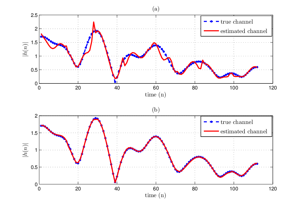
Clearly, when initialized with the “pilot-only DA’’ estimates1111
11
See section IV-B for more details about the pilot-assisted initialization process., the iterative algorithm is able to track the channel variations more accurately. Therefore, as clearly seen from Fig. 3(b), the “hybrid” EM-based SNR estimator exhibits paramount performance improvements especially for moderate to high SNR levels. Fig. 3(b) also highlights the advantage of performing IHD since the “hybrid-IHD” EM-based estimator is almost equivalent, over the entire SNR range, to the “completely DA” estimator which assumes all the symbols to be perfectly known. Even more, both estimators ultimately coincide with the CRLB which quantifies theoretically the best achievable performance ever. Fig. 3(b) also reveals that IHD yields more accurate SNR estimates than FHD and, therefore, the latter will not be considered in the remaining simulations. The “completely-NDA” EM-based estimator with SD, IHD, and FHD was also included in Fig. 3(a) to have these preliminary comparisons exhaustive and to motivate the use of the “pilot-only” DA estimates in initialization. Thus, in the remaining simulations we will focus on the “hybrid” EM-based estimator with SD and IHD only. Yet, we will keep using the “completely DA” estimator and the CRLB as ideal benchmarks.
Now, we will compare our new “hybrid’’ estimator against the only reported work1212
12
Note also that, using exhaustive computer simulations, we have demonstrated the clear superiority of our new ML estimators against other state-of-the-art techniques developed for constant channels [References, References, References] and time-varying channels [References, References]. The results were not included in this paper due to lack of space. on EM-based ML SNR estimation over time-varying channels introduced by A. Wiesel et al. in [References]. Using the initials of its authors’ names, we will henceforth designate it as “WGM”. This estimator was originally derived for single-input single output (SISO) systems. Thus, it can be directly applied at the output of each antenna element in order to estimate the instantaneous SNR in SIMO configurations. Yet, it can also be easily modified to take advantage of the antenna gain offered by SIMO systems experiencing uniform noise. In fact, over each antenna branch, the SISO WGM algorithm yields two estimates; one for the signal power, , and the other for the noise power, . The individual estimates can be averaged over the receiving antenna elements to provide a more refined estimate, , for the unknown noise power. The SIMO-enhanced WGM estimator over each antenna branch, referred to hereafter as the “WGM-SIMO” estimator, is then redefined as .

In Fig. 5, we compare our “hybrid” EM-based estimator (with , i.e., SISO) against WGM in terms of complex channel tracking capabilities and noise variance estimation accuracy over 5000 Monte-Carlo runs (i.e., 5000 consecutive observation windows each of size ). The reason behind considering such a very large number of observation windows — although it does not allow one to distinguish the true channel from its estimates — is to show that our estimator always converges to the global maximum. This can be, in fact, easily deduced by inspecting the noise variance estimates in the same figure. In plain English, under complex time-varying channels, the multidimensional LLF has many local maxima (i.e., multimodal) and the WGM estimator gets trapped into one of them due to its initialization issues. Therefore, as seen from Fig. 5(c), it is not able to estimate the noise variance over almost all the observation windows. Owing to our new proper initialization procedure, however, our “hybrid” EM-based estimator enjoys guaranteed global optimality and thus returns very accurate noise variance estimates over all the observation windows. Consequently, in contrast to WGM, it achieves the DA CRLB as shown in Fig. 6. Most remarkably, the “hybrid” algorithm is able to do so with of the transmitted symbols being completely unknown (corresponding to a pilot insertion rate of as advocated by the signalling standard specifications of the LTE uplink).


Fig. 7 depicts the performance of WGM-SIMO and the different versions of our estimator over three SIMO configurations (i.e., ). First, by inspecting the behaviour of the WGM estimator across the three subfigures, it is seen that the performance of its SIMO-enhanced version improves remarkably with the number of receiving antenna elements. For instance, at the typical value of the average SNR dB, it is seen from Figs. 7(a) and (b) that the variance of this estimator is reduced by a factor of when the number of antennae is doubled from to . The same improvements hold — although with a slightly smaller factor of — by further doubling the array size from to . Such improvements are actually due to the antennae gain only. Indeed, since WGM-SIMO is not able to exploit the antenna diversity, it is substantially outperformed even by our “completely-NDA-SD” estimator, for low-to-medium SNR levels. Here, we make a clear difference between the two concepts of antennae gain and diversity. The former is actually inherent to all SIMO systems experiencing uniform noise across the antenna elements (under correlated or uncorrelated channels). In this case, averaging the independent estimates of the same noise power produces a new estimate whose variance is always shrunk by a factor of , improving thereby the final estimates of the per-antenna SNRs.
Antennae diversity, however, is another more interesting feature of SIMO systems. Fully exploiting the antennae diversity consists in optimally combining the multiple independently-fading copies of the received signal in order to detect each of the transmitted symbols correctly. By solving the ML criterion, our “hybrid-SD” (or “hybrid-IHD”) EM-based estimator takes indeed advantage of the available spatial diversity to accurately estimate (or detect) the unknown transmitted symbols. For these reasons and owing to our proper initialization procedure, the “hybrid” EM-based algorithm (with SD or IHD) outperforms by far WGM-SIMO over the entire SNR range.
From another perspective, the performance improvements that are obtained by fully exploiting the antennae gain together with the antennae diversity offered by SIMO over SISO systems can be easily appreciated by comparing Figs. 7 and 6. For instance, at the typical average SNR value of dB, the NMSE of the “hybrid” EM-based estimator is substantially reduced by a factor as high as using antenna branches compared to SISO.
So far, all the simulations where conducted under a normalized Doppler frequency of corresponding to a maximum Doppler shift Hz with the sampling rate of LTE systems s. This translates into a medium user velocity Km/h at a carrier frequency GHz with being the speed of light. Therefore, we plot in Fig. 8 the performance of the newly derived ML estimator for higher normalized Doppler frequencies.

It is seen from this figure that both the “completely DA” and “hybrid” estimators succeed in accurately estimating the SNR reaching thereby the DA CRLB even at high Doppler frequencies. In Fig. 8(d), for instance, the normalized Doppler frequency is as high as corresponding to a maximum Doppler frequency of Hz (translating to a user velocity as high as Km/h at GHz). Within the same context, we emphasize the fact that the sizes of the local approximation windows, and , for both the “hybrid” estimator and the “pilot-only DA” that is used to initialize it should be properly selected according to the Doppler range as shown in Table I.
| 112 | 56 | 4 | 4 | |
| 28 | 28 | 4 | 4 | |
| 28 | 14 | 4 | 4 | |
| 14 | 7 | 2 | 4 |
In practice, the Doppler frequency can be estimated from the samples received at the pilot positions and the approximation window sizes are then selected accordingly. When designing these Doppler-dependent configurations, our primary goal was to obtain the lowest possible polynomial orders and which define the sizes of the two matrices that need to be inverted. Yet, it should be mentioned that these small-size matrices are predefined ones. Hence, in practice, they can be computed and inverted offline once for all, stored in memory, and then used in online estimation at no extra computational cost.
VI Conclusion
In this paper, we formulated and derived ML estimators for the instantaneous SNR over time-varying SIMO channels using local polynomial-in-time expansions. In the DA scenario, the ML estimator was derived in closed form, and so were its bias, its variance and the DA CRLB. In the NDA case, however, we proposed a ML solution that is based on the iterative EM concept and that is able to converge to the global maximum within very few iterations. Appropriate initialization is indeed guaranteed by applying the DA estimator over periodically inserted pilot symbols. Furthermore, the new estimator is applicable to any channel fading type over a relatively large Doppler range and for any linearly-modulated signal (i.e., PSK, PAM, QAM). Finally, it is able to reach the CRLB over a wide SNR range and outperforms by far the new SIMO-extended version of the only work published so far, to the best of our knowledge, on EM-based ML SNR estimation over SISO time-varying channels.
Appendix A
Proof of Theorem 1
To begin with we define, , as the orthogonal projector on the signal subspace (of each antenna element) corresponding to the local DA approximation window (of size ) as follows:
| (59) |
where and is a diagonal matrix that contains the known transmitted symbols on its main diagonal, i.e., . Note here that is different from that is defined earlier right after (19) as the orthogonal projector over the signal subspace (of the whole antennae array) corresponding to the local DA approximation window.
We associate to the operator as the projector onto the orthogonal complement of the corresponding signal subspace.
Now recall that the estimates of the antenna’s channel coefficients corresponding to the local DA approximation window, , are obtained as:
| (60) |
where is obtained by extracting the corresponding block from obtained in (17) to yield:
| (61) |
Therefore, by substituting (61) back into (60), it follows that:
| (62) |
Moreover, from (60), we readily see that the component, , of is obtained as the inner product between the row of (i.e., the vector and leading to:
| (63) |
Now, recall from (22) that the estimated SNR in the DA mode is given:
| (64) |
and owing to (63), the numerator of the estimated SNR in (64) (denoted herafter as “”) is expressed as follows:
| (65) |
By further noticing that:
| (66) |
it follows that:
| (67) |
Then, by using (62) and recalling the fact that , we have:
| (68) |
Then, by substituting (68) in (67), it follows that:
| (69) |
On the other hand, the denominator of the SNR estimate in (64) is given by:
| (70) |
and since is obtained from (19) as:
| (71) |
with , we obtain by substituting (71) back in (70) the following result:
| (72) |
Raclling that , it can be easily shown that:
| (73) | |||||
Now, let be a vector that contains all the received samples over the antenna elements. Thus, the SNR estimate at the antenna element is obtained from (69) and (73) as follows:
| (74) |
Next, in order to find the distribution of , we will first proceed to finding the distributions of and separately. To that end, recall first from (13) that (when ):
| (75) |
where with being the identity matrix. Therefore, the mean and covariance matrix of are given by:
| (76) | |||||
| (77) |
Therefore, if we define the following transformed random vector:
| (78) |
then we immediately have . Now, since is a Hermetian matrix then it can be diagonalized as follows:
| (79) |
where is a unitary matrix (i.e., ) and is a diagonal matrix that contains the eigenvalues of (which are all positive). Moreover, since , we have:
| (80) |
which means that or equivalently for and, therefore, { or for }. However, since is a Vondermende matrix, it is of (full) rank and since is a diagonal matrix, it follows that is also of rank . Consequently, the projection matrix is also of rank and, therefore, we have exactly eigenvalues that are equal to one and the others are exactly zero. In the following we assume (without loss of generality) that the first eigenvalues are non-zero. That is for and for , which means:
Now, combining (78) and (79) and using the fact that is a unitary matrix, it follows that:
| (82) |
By further defining the transformed received vector:
| (83) |
and again using the fact that is a unitary matrix, it follows that and:
| (84) |
in which is used to denote the element of the vector and where the last equality follows from the fact that only the first diagonal entries of are non-zero and are all equal to one [see (Appendix A
Proof of Theorem 1)]. By plugging (84) back into (69), we obtain:
| (85) |
In addition, since the vector is Gaussian distributed according to , then its elements are independent and Gaussian distributed according to:
| (86) |
where is used to denote the column of the matrix . Consequently, is a sum of the squares of independent Gaussian random variables all having unit variance but non-zero means and, therefore, is chi-square distributed with degrees of freedom and noncentrality parameter:
| (87) | |||||
where the last quality follows from the fact that the first diagonal entries of are equal to one and the remaining diagonal ones are all equal to zero. Furthermore, by recalling that and that , it follows that:
| (88) | |||||
In conclusion, we have is a noncentral chi-distributed, i.e.:
| (89) |
with degrees of freedom and noncentrality parameter .
Now recall from (73) that the denominator is equal to:
| (90) |
Similarly, by noticing that is of rank and recurring to equivalent manipulations, it can be shown that the denominator can be rewritten in the following form:
| (91) |
where are the components of another transformed observation vector which are Gaussian distributed with zero mean and unit variance. Hence, the random variable follows a central chi-distribution [36], i.e.:
| (92) |
with degrees of freedom. Moreover, and involve projection onto a signal subspace and its orthogonal complement, respectively, and hence the two chi-distributed random variables are independent. In conclusion, we have:
| (93) |
which implies that the scaled estimated SNR over each antenna element verfies:
| (94) |
where is a noncentral distribution with a noncentrality parameter and degrees of freedom and .
Appendix B
Details about the derivation of the bias and the variance
By using , it follows immediately from (23) that:
| (95) |
Moreover, by substituting , and in (24), it follows that:
| (96) |
Then, by recognizing some easy simplifications, one obtains:
| (97) |
Therefore, by using (97) in (95), it follows that:
| (98) |
Now, (27) is obtained in the same way, i.e., first by substituting , and in (25) (with some easy simplifications) and then injecting the result in the following identity:
| (99) |
The exact bias of , which is given by , is then easily obtained from (98) as given by (III-B). Furthermore, it follows from (98) that:
| (100) | |||||
which simply implies that:
| (101) |
is indeed an unbiased estimator of the per-antenna SNRs. By using the identity for any random variable and any real number , the variance of is given by:
| (102) |
which is further simplified using (27) in order to obtain the result in (III-B).
Appendix C
Derivation of the DA CRLB
To assess the performance of the new unbiased DA ML estimator, we need to compare its variance to a theoretical lower bound. Thus, we derive in this Appendix the corresponding DA CRLB. Here, for some reasons that are better clarified in sections IV and V, we are interested in comparing our estimators against the lowest possible bound (i.e., the best achievable performance). Without loss of generality, we hence consider an ideal scenario where all the transmitted symbols are assumed to be perfectly known (i.e., or equivalently ). Now, we define the following parameter vector:
| (103) |
where and denote the real and imaginary parts of the vector that contains the true channel coefficients over all the receiving antenna elements and the entire observation window. The CRLB for the DA SNR estimation over the antenna is given by:
| (104) |
where with being a diagonal matrix containing the transmitted pilot symbols and where denotes the Fisher information matrix (FIM) whose entries are defined as:
| (105) |
where
In (Appendix C
Derivation of the DA CRLB), ans are given by:
with for . Starting from (Appendix C
Derivation of the DA CRLB), we will now derive the analytical expression for the FIM.
In fact, by recalling that where and stand for the real and imaginary parts of , respectively, we can obtain the required partial derivatives in (105) as follows:
| (107) |
| (108) |
| (109) |
and
| (110) | |||||
Moreover, it is easy to verify that:
| (111) | |||||
for and with . Additionally, the expected values of the previously derived partial derivatives with respect to are given by:
| (112) | |||||
| (113) |
And it can be easily shown that:
| (114) | |||||
Now using:
| (115) |
we can finally derive the analytical expression for the FIM as follows:
| (116) |
which turns out to be a block-diagonal matrix whose inverse is straightforward. Moreover, by recalling that and , it is easy to verify that:
| (117) |
from which it can be shown that [38]:
and . Finally, by using this result, injecting (116)-(Appendix C
Derivation of the DA CRLB) in (104) and after some algebraic manipulations, a simple closed-form expression for the CRLB of the DA instantaneous SNR estimates is obtained as follows:
| (119) |
References
- [1] F. Bellili, R. Meftehi, S. Affes, and A. Stéphenne “Maximum likelihood SNR estimation over time-varying flat-fading SIMO channels,” in Proc. of IEEE ICASSP, Florence, Italy, May 2014, pp. 6523-6527.
- [2] N. C. Beaulieu, A. S. Toms, and D. R. Pauluzzi, “Comparison of four SNR estimators for QPSK modulations,” IEEE Commun. Lett,, vol. 4, no. 2, pp. 43-45, Feb. 2000.
- [3] K. Balachandran, S. R. Kadaba, and S. Nanda, “Channel quality estimation and rate adaption for cellular mobile radio,” IEEE J. Sel. Areas Commun., vol. 17, no. 7, pp. 1244-1256, July 1999.
- [4] T. A. Summers and S. G. Wilson, “SNR mismatch and online estimation in turbo decoding,” IEEE Trans. Commun., vol. 46, no. 4, pp. 421-423, Apr. 1998.
- [5] N. Nahi and R. Gagliardi, “On the estimation of signal-to-noise ratio and application to detection and tracking systems,” University of Southern California, Los Angeles, EE Report 114, Jul. 1964.
- [6] T. Benedict and T. Soong, “The joint estimation of signal and noise from sum envelope,” IEEE Trans. Inf. Theory, vol. 13, no. 3, pp. 447-454, Jul. 1967.
- [7] D. R. Pauluzzi and N. C. Beaulieu, “A comparison of SNR estimation techniques for the AWGN channel,” IEEE Trans. Commun., vol. 48, no. 10, pp. 1681-1691, Oct. 2000.
- [8] W. Gappmair, R. Lopez-Valcarce, and C. Mosquera, “Cramér-Rao lower bound and EM algorithm for envelope-based SNR estimation of nonconstant modulus constellations,” IEEE Trans. Commun., vol. 57, no. 6, pp. 1622-1627, Jun. 2009.
- [9] M. Turkboylari and G. L. Stuber, “An efficient algorithm for estimating the signal-to-interference ratio in TDMA cellular systems,” IEEE Trans. Commun., vol. 46, no. 6, pp. 728-731, Jun. 1998.
- [10] P. Gao and C. Tepedelenlioglu, “SNR estimation for non-constant modulus constellations,” IEEE Trans. Signal Process., vol. 53, no. 3, pp. 865-870, Mar. 2005.
- [11] R. Lopez-Valcarce and C. Mosquera, “Sixth-order statistics-based non-data-aided SNR estimation,” IEEE Commun. Lett., vol. 11, no. 4, pp. 351-353, Apr. 2007.
- [12] M. Àlvarez-Diaz, R. Lopéz Valcare, and C. Mosquera “SNR estimation for multilevel constellations using higher-order moments,” IEEE Trans. Signal Process., vol. 58, no. 3, pp. 1515-1526, Mar. 2010.
- [13] A. Wiesel, J. Goldberg, and H. Messer, “Non-data-aided signal-to-noise estimation,” in Proc. ICC, vol. 1, New York City, NY, USA, 2002, pp. 197-201.
- [14] A. Das (Nandan), “NDA SNR estimation: CRLB and EM based estimators”, in Proc. IEEE TENCON, Hyderabad, India, 2008, pp. 1-6.
- [15] W. Gappmair, R. Lopez-Valcarce, and C. Mosquera, “ML and EM algorithm for non-data-aided SNR estimation of linearly modulated signals,” in Proc. IEEE Symp. Commun. Syst., Graz, Austria, 2008, pp. 530-534.
- [16] A. Stéphenne, F. Bellili, and S. Affes, “Moment-based SNR estimation over linearly-modulated wireless SIMO channels,” IEEE Trans. Wireless Commun., vol. 9, no. 2, pp. 714-722, Feb. 2010.
- [17] A. Stéphenne, F. Bellili, and S. Affes, “Moment-based SNR estimation for SIMO wireless communication systems using arbitrary QAM,” in Proc. 41st Asilomar Conference on Signals, Systems and computers, Pacific Grove, CA, USA, 2007, pp. 601-605.
- [18] M. A. Boujelben, F. Bellili, S. Affes, and A. Stéphenne, “EM Algorithm for Non-Data-Aided SNR Estimation of Linearly-Modulated Signals over SIMO Channels”, in Proc. of IEEE GLOBECOM, Honolulu, Hawaii, USA, 2009, pp. 1-6.
- [19] M. A. Boujelben, F. Bellili, S. Affes, and A. Stéphenne, “SNR estimation over SIMO channels from linearly modulated signals,” IEEE Trans. Signal Process., vol. 58, no. 12, pp. 6017-6028, Dec. 2010.
- [20] A. Das and B. D. Rao, “SNR and noise variance estimation for MIMO systems,” IEEE Trans. Signal Process., vol. 60, no. 8, pp. 3929-3941, Aug. 2012.
- [21] T. Gao and B. Sun, “A high-speed railway mobile communication system Based on LTE,” in Proc. ICEIE 2010, vol. 1, Kyoto, Japan, 2010, pp. 414-417.
- [22] Morelli, M. Moretti, M. Imbarlina, and G. Dimitriou, N., “Low complexity SNR estimation for transmissions over time-varying flat-fading channels,” in Proc. IEEE WCNC, Budapest, Hungary, 2009, pp. 1-4.
- [23] H. Abeida,“Data-aided SNR estimation in time-variant Rayleigh fading channels,” IEEE Trans. Signal Process., vol. 58, no. 11, pp. 5496-5507, Nov. 2010.
- [24] A. Wiesel, J. Goldberg, and H. Messer-Yaron, “SNR estimation in time-varying fading channels,” IEEE Trans. Commun., vol. 54, no. 5, pp. 841-848, May 2006.
- [25] F. Bellili, A. Stéphenne, and S. Affes, “SNR estimation of QAM-modulated transmissions over time-varying SIMO channels,” in Proc. IEEE Int. Symp. Wireless Commun. Syst., Reykjavik, Iceland, 2008, pp. 199-203.
- [26] A. Stéphenne, F. Bellili, and S. Affes, “A decision-directed SNR estimator for QAM signals over time-varying SIMO channels,” in Proc. of IEEE 24th Biennial Symposium on Communications, Kingston, ON, Canada, June 2008, pp. 17-20.
- [27] A. P. Dempster , N. M. Laird, and D. B. Rubin “Maximum likelihood from incomplete data via the EM algorithm”, J. Royal Stat. Soc., vol. 39, no. 1, pp. 1-38, 1977.
- [28] J. A. C. Bingham “Multicarrier modulation for data transmission: An idea whose time has come”, IEEE Commun. Mag., vol. 28, no. 5, pp. 5-14, May 1990.
- [29] Z. Wang and G. B. Giannakis, “Wireless multicarrier communications: Where Fourier meets Shannon”, IEEE Signal Processing Mag., vol. 17, no. 3, pp. 29-48, May 2000.
- [30] P. A. Bello “Characterization of randomly time-variant linear channels”, IEEE Trans. Commun. Syst., vol. CS-11, no. 04, pp. 360-393, Dec. 1963.
- [31] F. Bellili, A. Stéphenne, and S. Affes, “Cramér-Rao bounds for NDA SNR estimates of square QAM modulated signals,” in Proc. IEEE WCNC, Budapest, Hungary, Apr. 2009.
- [32] F. Bellili , A. Stéphenne, and S. Affes, “Cramér-Rao lower bounds for NDA SNR estimates of square QAM modulated transmissions,” IEEE Trans. Commun., vol. 58, no. 11, pp. 3211-3218, Nov. 2010.
- [33] F. Bellili, N. Atitallah, S. Affes, and A. Stéphenne, “Cramér-Rao lower bounds for frequency and phase NDA estimation from arbitrary square QAM-modulated signals,” IEEE Trans. Signal Process., vol. 58, no. 9, pp. 4517-4525, Sep. 2010.
- [34] C. Anton-Haro, J. A. R. Fonollosa, C. Fauli, and J. R. Fonollosa, “On the inclusion of channel’s time dependence in a hidden Markov model for blind channel estimation,” IEEE Trans. Veh. Technol., vol. 50, no. 3, pp. 867-873, May 2001.
- [35] S. M. Kay, Fundamentals of Statistical Signal Processing: Vol. 1—Estimation Theory, Englewood Cliffs, NJ: Prentice Hall, 1993.
- [36] S. M. Kay, Fundamentals of Statistical Signal Processing: : Vol. 2—Detection Theory. Englewood Cliffs, NJ: Prentice-Hall, 1998.
- [37] 3GPP TS 36.211: 3rd Generation Partnership Project; Technical Specification Group Radio Access Network; Evolved Universal Terrestrial Radio Access (E-UTRA); Physical Channels and Modulation.
- [38] K. B. Petersen and M. S. Pedersen, The Matrix Cookbook, Lyngby, Denmark: Technical Univ. of Denmark, 2006.