Unconventional localisation transition in high dimensions
Abstract
We study non-interacting systems with a power-law quasiparticle dispersion and a random short-range-correlated potential. We show that, unlike the case of lower dimensions, for there exists a critical disorder strength (set by the band width), at which the system exhibits a disorder-driven quantum phase transition at the bottom of the band, that lies in a universality class distinct from the Anderson transition. In contrast to the conventional wisdom, it manifests itself in, e.g., the disorder-averaged density of states. For systems in symmetry classes that permit localisation, the striking signature of this transition is a non-analytic behaviour of the mobility edge, that is pinned to the bottom of the band for subcritical disorder and grows for disorder exceeding a critical strength. Focussing on the density of states, we calculate the critical behaviour (exponents and scaling functions) at this novel transition, using a renormalisation group, controlled by an expansion. We also apply our analysis to Dirac materials, e.g., Weyl semimetal, where this transition takes place in physically interesting three dimensions.
pacs
72.15.Rn, 64.60.a, 03.65.Vf, 72.20.EeI Introduction
Decades of studies of transport and metal-insulator transitions in disordered materials have resulted in well-established qualitative pictures of these phenomena[1, 2, 3]. The conventional wisdom prescribes that single-particle transport and localisation phenomena can be understood by considering electron scattering only close to the Fermi surface; elastic scattering through states far from the Fermi surface is believed to only finitely renormalise the parameters of the low-energy excitations, without any qualitative consequences.
However, such qualitative picture is not always correct, as has been known since the pioneering works [4, 5, 6], which showed that transport and localisation in materials with Dirac quasiparticle dispersion are qualitatively affected by elastic scattering between all states, even far from the Fermi surface. For example, in three-dimensional (3D) Dirac materials the scattering contribution from the full band is known to lead to a disorder-driven phase transition between weak- and strong-disorder phases[5, 6]. This picture has been extensively elaborated on and is now widely accepted[7, 8, 9, 10, 11, 12, 13, 14].
In our recent paper [11] we have demonstrated [in a controlled renormalisation-group (RG) analysis] that such single-particle interference far from the Fermi surface is not specific to Dirac materials; it dramatically affects transport and the metal-insulator transition in any semiconductor or a semimetal in sufficiently high dimensions. This applies, in particular, in the case of the quadratic quasiparticle dispersion in dimensions and in the case of Dirac Hamiltonians in dimensions .
As discussed in Ref. 11, in a material with quasiparticle kinetic energy
| (1) |
in the dimensions quasiparticle states near the bottom of the band experience renormalisations from all the other states in the band in the presence of a random short-range-correlated potential. This leads to a quantum phase transition already in the single-particle properties as a function of the disorder strength, as summarised in Fig. 1. Depending on whether the disorder strength is above or below a critical value , the effects of quenched random potential grow or decrease at small momenta, respectively.

As a result, the density of states close to the bottom of the band exhibits a critical behaviour as a function of disorder strength, unlike its smooth dependence on both energy and disorder strength in the more familiar case of .
A well-known example of materials corresponding to the case of is the recently realised[15, 16, 17, 18, 19] Weyl semimetals, 3D materials with Dirac-type linear quasiparticle dispersion[20, 21] (, ). While localisation in a single-valley Weyl semimetal due to potential disorder is forbidden by symmetry[21, 22], the weak-to-strong-disorder transition persists and manifests itself in, e.g., the critical behaviour of the conductivity , that has been analysed microscopically for small but finite doping in our recent paper, Ref. 11, and also for zero doping in Refs. 23, 5, 24. The critical behaviour of the density of states for 3D Dirac quasiparticles has been studied in Refs. 14, 5, 9, 24.
As we have also demonstrated there, disordered semiconductors with the conventional quadratic quasiparticle spectrum in dimensions are also characterised by a critical disorder strength. Although one might think that such predictions are of purely academic interest, the properties of high-dimensional semiconductors are observable experimentally: a disordered semiconductor with the quadratic spectrum in arbitrary dimension can be mapped[25, 26] to a one-dimensional periodically kicked quantum rotor, similar to those already realised[27, 28, 29] in cold atomic gases to simulate Anderson localisation in 1D and 3D. Thus, such kicked rotors present a flexible experimental platform for observing unconventional localisation physics of high-dimensional semiconductors explored here. Also, our results can be tested in numerical simulations of Anderson localisation transition in high dimensions[30, 31, 32, 33] close to the band edge.
In contrast, in subcritical dimensions, , the RG analysis shows that the effects of disorder grow at smaller momenta and are most important close to the Fermi energy. This is consistent with the common assumption, widely used in the literature[1, 2, 34], that one may consider only quasiparticles near the Fermi surface when describing transport and metal-insulator transitions in metals and conventional semiconductors.
In this paper we further study the weak-to-strong-disorder transition in materials with , such as high-dimensional semiconductors and semimetals, particularly focussing on the disorder-averaged density of states.
We conclude the Introduction by summarising our key results and experimental predictions. Then in Sec. II we introduce the model for a semiconductor with a power-law dispersion and short-range-correlated disorder. In Sec. III we discuss the tails of the density of states that emerge below the edge of the conduction band due to rare fluctuations of the disorder potential (Lifshitz tails). In Sec. IV we develop a perturbation theory for the states in the conduction band and obtain divergent contributions to the effective disorder strength for dimensions higher than critical. Sec. V is devoted to the RG treatment of the problem, controlled by an -expansion. In Sec. VI we study the disorder-averaged density of states, the mobility threshold, and the localisation length using scaling analysis and complementary microscopic calculations. Sec. VII deals with the density of states in Weyl semimetal. We conclude in Sec. VIII with a summary and a discussion of open questions.
Summary of the results
The key features of our findings for quadratically and linearly dispersing semiconductors and Dirac semimetals is encoded in the diagram in Fig. 1. As summarised there, for the effects of random potential grow at long wavelengths relative to the kinetic energy, which, if allowed by symmetry and if (in addition to ), leads to a mobility threshold between low-energy localised and high-energy delocalised states. In stark contrast, for and disorder strength weaker than the critical , the effective disorder strength decreases relative to the kinetic energy for low momenta. On the other hand, disorder stronger than critical grows at long wavelengths, leading to a finite density of states and localisation (if permitted by symmetry). This leads to a disorder-driven quantum phase transition that underlies all our results.
We study this transition using scaling analysis and a complementary microscopic calculation, based on the RG-analysis, controlled by
| (2) |
expansion, and compute a number of physical observables.
I.0.1 Density of states
We find that the density of states exhibits the critical behaviour (which has been proposed previously in Ref. 14 for 3D Dirac quasiparticles)
| (3) |
with the limiting cases summarised in Fig. 2. Here and are respectively the dynamical and the correlation length critical exponents and is a universal scaling function.
There are three different regimes of the critical behaviour of the density of states .

Close to the critical disorder strength, , the density of states is given by a power-law and is disorder-strength-independent. For low energies and subcritical disorder () the energy dependence of the density of states coincides with that of a disorder-free system, but with a disorder-dependent enhancing prefactor that diverges as the transition is approached (): , Fig. 3. For low energies and strong disorder (), the density of states is smeared by disorder and is thus finite and only weakly energy-dependent.

For a semiconductor [a material with the quasiparticle dispersion (1) in the orthogonal symmetry class] we find the critical exponents and in the RG framework with small in the one-loop approximation:
| (4) | |||
| (5) |
For instance, in the case , , which can be particularly easily realised numerically, using the tight-binding model on a square lattice, and also simulated in quantum-kicked-rotor systems, Eqs. (4) and (5) give and . We emphasise, however, that the respective is not small and may require a similar high-loop calculation to accurately describe experimentally and numerically observed values of the exponents and .
Disorder not only affects the states in the conduction band of a semiconductor, but also leads to the formation of “Lifshitz tails”[35, 36, 37, 38], deeply localised states below the edge of the conduction band that occur due to rare fluctuations of the disorder potential.
We find that the nature of the Lifshitz tail depends crucially on whether or not the dimension is above or below critical, in the case of Gaussian disorder considered in this paper. Unlike the conventional case of low dimensions, broadly studied in the literature[35, 36, 37, 38], for the density of states just below the edge of the conduction band is exponentially suppressed at weak disorder and weakly depends on energy:
| (6) |
where is a constant of order unity.
We note, that the position of the band edge is shifted upon renormalisation, and we define the energy in the conduction band [cf. Eq. (3)], as well as Lifshitz tail relative to the renormalised edge.
Because of the exponential suppression of the tail in the limit of weak disorder or small , here the conduction band can be clearly distinguished from the Lifshitz tail in these limits, and the band edge is clearly defined 11 1 Throughout the paper, by the “bottom of the band” we mean the disorder-renormalised edge of the band, not accounting for the rare-regions effects that lead to the formation of Lifshitz tails (exponentially suppressed in ).. This should be contrasted with the conventional case of low dimensions, where the contribution of the Lifshitz tail can be significant near the bottom band, and thus the band edge is not well-defined.
I.0.2 Mobility thresholds and localisation length
Another profound consequence of single-particle interference effects in high dimensions is the unusual behaviour of the mobility threshold [the energy separating localised and delocalsed states] as a function of the disorder strength, in contrast to its conventional smooth behaviour in low dimensions. Slightly above the critical dimension () the mobility threshold is pinned to the bottom††footnotemark: of the band for subcritical disorder, , and rapidly grows with disorder strength for stronger disorder, , as illustrated in Figs. 4 and 2.

Furthermore, we show that the critical properties of the localisation transition in higher dimensions are richer than those below the critical dimension. According to the conventional wisdom, in the vicinity of the Anderson transition localised wavefunctions are characterised by a localisation length that diverges at the transition as
| (7) |
with a finite mobility threshold in the conduction band and a correlation-length exponent which is believed to be universal and to depend only on the dimension and the symmetry class, provided the latter allows for localisation. In particular, the exponent is believed to be independent of the quasiparticle dispersion in a given symmetry class.
In contrast, we find that the phenomenology in high dimensions () is richer. For , the critical behaviour is indeed described by Eq. (7) with a universal exponent , but with the mobility threshold vanishing as approaches [see also Eq. (3)],
| (8) |
and remaining zero for . For , however, the localisation length of the state diverges according to
| (9) |
with the universal exponent given by Eq. (4) in the limit of small .
Finally, for subcritical disorder, , the localisation length changes rapidly in a small energy interval, in which the conduction band crosses over to the Lifshitz tail. Indeed, we demonstrate that in the conduction band quasiparticle states are delocalised for , because the disorder strength vanishes upon renormalisation, while in the tail the localisation length is of the order of the correlation length of the potential.
I.0.3 Weyl semimetal
In addition to semiconductors with a scalar Hamiltonian of the kinetic energy of quasiparticles, we study the density of states in Weyl semimetal, where electrons are characterised by the Dirac-type dispersion .
Although there is no localisation in Weyl semimetal in the presence of smooth random potential, such system still exhibits the disorder-driven phase transition, manifested in, e.g., the density of states, as summarised in Figs. 5 and 6.


These results are obtained using an RG approach (similar to the calculation for a semiconductor) controlled by small with set at the end of the calculation.
II Model
As discussed in the Introduction, in this paper we study a single-particle problem in the presence of a quenched random potential and analyse the effects of the latter on the single-particle density of states and other related properties.
We consider a semiconductor with the quasiparticle Hamiltonian
| (10) |
in the conduction band, where is the kinetic energy of a quasiparticle with momentum , and is a weak Gaussian disorder potential with zero average and a correlation function
| (11) |
We take the latter to decay quickly on distances larger than the characteristic length .
If the disorder potential is caused by neutral impurities, lattice defects or vacancies, is of the order of the typical size of these impurities or defects. Disorder in semiconductors and semimetals can be represented also by screened Coulomb impurities[39], in which case is given by the screening radius. For doped semiconductors the screening is determined by the concentration of dopants, for intrinsic semiconductors– by electrons thermally activated from the valence band or by electron and hole puddles that emerge due to the fluctuations of the impurity concentration[39, 40, 41].
In what follows we refer to as the “impurity size”. As we show in Sec. IV, the scale serves as an ultraviolet momentum cutoff for the interference effects in the conduction band, which lead to the renormalisation of the states close to the bottom††footnotemark: of the band.
If processes under consideration involve momentum states with wavelengths exceeding , the disorder can be considered -correlated,
| (12) |
where .
In this paper, in the case of a semiconductor, we neglect electron scattering to the valence band, valid, for instance, in the case of a sufficiently large band gap , separating the conduction and the valence bands, which exceeds the width of the conduction band or the disorder-determined ultraviolet (UV) energy cutoff .
However, in the case of Weyl semimetal, there is no band gap, and we therefore take into account scattering between the conduction and the valence bands.
Throughout the paper we assume that the dimension is integer, while the exponent can be fractional. In particular, the parameter
| (13) |
can be arbitrarily small.
III Lifshitz tails and rare-regions effects in high dimensions
While typical fluctuations of the disorder potential can be treated in a perturbative RG analysis, discussed in the main part of the manuscript, rare regions of space with large disorder potential require more subtle non-perturbative analysis and lead to the formation of states with arbitrarily low energies below the edge of the conduction band, known as “Lifshitz tail”. Understanding the structure of such tails is indispensable for a complete description of single-particle states in disordered semiconductors.
Lifshitz tails have been extensively studied for conventional semiconductors[35, 36, 37, 38], corresponding to low dimensions . For quadratic quasiparticle dispersion it has been estimated for the density of states deep in the Lifshitz tail in dimension that , in the case of Gaussian disorder, considered in this paper (in principle, the result is non-universal and will differ for non-Gaussian disorder).
In what immediately follows we use phenomenological arguments, similar to those of Refs. 35, 36, 37, 38, to obtain the density of states in the Lifshitz tail in high dimensions, . We find that the structure of the tail is dramatically different from the case of low dimensions, again uncovering the crucial role played by the critical dimension . In particular, for weak disorder or small the density of states weakly depends on energy, , and is exponentially small for sufficiently small energies , including , which is of particular interest to us.
The states with large negative energies occur due to rare regions with large negative disorder potential that trap particle states.
The distribution of the average disorder potential in a spatial region of volume is described by the Gaussian probability density
| (14) |
as follows from Eq. (12).
The density of states at a large negative energy in a semiconductor with quasiparticle dispersion is determined by the fluctuations of the potential on length scales that exceed the characteristic impurity size [the correlation radius of the function ]. We thus consider the contribution of such rare regions of deep random potential wells of characteristic size to the density of states.
States with energy and typical linear size occur due to the potential fluctuations in spatial regions of volume , where estimates the kinetic energy of the zero-point motion that raises the energy above , the bottom of the potential well. The density of states is determined by the “optimal fluctuation” [35, 36, 37, 38], i.e. the value of which maximises
| (15) |
The dominant contribution to the density of states is thus determined by the competition between large scales , that lower the zero-point kinetic energy, and small scales , for which potential fluctuations are more probable.
In subcritical dimensions, , the maximum is achieved at , leading to the conventional result
| (16) |
where is a constant of order unity. The density of states (16) has been obtained previously for conventional semiconductors [35, 36, 37, 38].
In high dimensions, , the expression (15) has no maximum at finite and grows infinitely as . Thus, the density of states in high dimensions is determined by the shortest microscopic length scales. The minimal scale in the model is the “impurity size” . Inserting in Eq. (15), we obtain
| (17) |
Eqs. (16) and (17) correctly describe the densities of states in low () and high () dimensions respectively, provided the respective exponentials are significantly smaller than unity. While Eq. (16) thus applies in low dimensions only for sufficiently large negative energies , Eq. (17) describes the density of states in the Lifshitz tail in high dimensions for all negative energies provided the disorder is weak enough, .
Our result, Eq. (17), thus shows that in high dimensions the density of states weakly depends on energy for and decays exponentially otherwise.
Gapless semiconductors. Since Eq. (17) applies for all energies below the bottom††footnotemark: of the band, it can be used to describe the smearing of the density of states at the degeneracy point in gapless semiconductors, i.e. materials where the conduction and the valence bands touch, such as Weyl semimetals or graphene. In these materials there is no band gap, so the expression (17) can be used only for , i.e. in the bottom of the conduction band (the top of the valence band). Indeed, for , , and , Eq. (17) gives the density of states in Weyl semimetal, recently obtained in Ref. 42.
IV Perturbation theory in the conduction band
In Sec. III we addressed the density of states below the edge of the conduction band due to rare fluctuations of the disorder potential. Let us now consider the states in the conduction band, where it is sufficient to consider the typical fluctuations of the random potential.
IV.1 Phenomenological argument for the existence of the critical dimension
Before turning to more technical perturbative and RG analyses, we assess of the role of quenched disorder using phenomenological scaling arguments. The importance of the random potential to a singe-particle state of momentum can be assessed by comparing the kinetic energy with the typical fluctuation of the (zero-mean) random potential, averaged over the volume , set by the de Broglie wavelength .
For , the ratio [, with being the dimensionless measure of disorder strength, introduced in Eq. (35) below] vanishes with reduced momentum, which reflects the irrelevance of disorder (in RG parlance) in higher dimensions.
In contrast, for the effects of disorder grow at small momenta. For (in addition to ), we expect the localisation of particles with sufficiently low momenta , such that the kinetic energy is of the order of the characteristic disorder potential fluctuation . This allows us to estimate the mobility threshold in lower dimensions:
| (18) |
Although the above phenomenological argument allows one to predict the existence of the critical dimension and qualitatively different effects of disorder in dimensions and , such argument neglects elastic scattering of the states with characteristic momentum through the states .
We show below that such large-momentum scattering is important in higher dimensions, but may be neglected in the dimensions below critical. Indeed, sufficiently below the critical dimension [in the limit ], the phenomenological estimate (18) of the mobility threshold is accurate and coincides with the result [Eq. (63) below] of a rigorous RG calculation. However, when approaching the critical dimension (), the above estimate, Eq. (18), is no longer accurate, as elastic scattering between all states in the band needs to be taken into account.
IV.2 Perturbative correction to the disorder strength
In what immediately follows we apply perturbation theory to show that sufficiently below critical dimensions, , the quasiparticle transport in a weakly disordered semiconductor is dominated by the scattering between states in a narrow momentum shell, , whereas close to or above the critical dimensions, , scattering in a large band of momenta , up to the UV cutoff , is important.
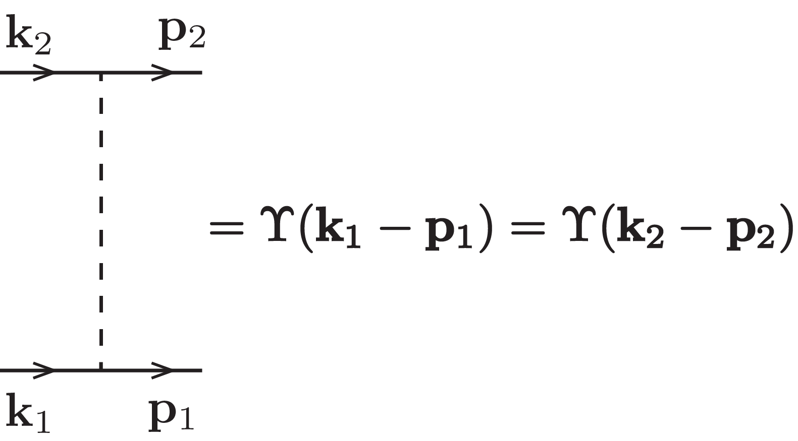
In the leading order in the disorder strength, the effect of large-momentum scattering () on states with small momenta can be illustrated by the renormalisation of the impurity line, Fig. 7, mimicked diagramatically in Fig. 8 and estimated as

| (19) |
where is the Fourier-transform of the disorder correlation function , Eq. (12), and is the kinetic energy of a quasiparticle with momentum .
For short-range-correlated disorder, which we consider in this paper, the function decays fast beyond the cutoff momentum , and the renormalisation of the impurity line can be rewritten in terms of modification of the disorder strength , Eq. (12),
| (20) |
where and is the area of a unit sphere in a -dimensional space.
IV.2.1 Subcritical dimensions
Consistent with the phenomenological analysis of Subsection IV.1, in the dimensions the integral in Eq. (20) is dominated by momenta near the lower limit, and
| (21) |
where we have introduced the quasiparticle mean free path (cf. Appendix A for a detailed calculation of the mean free path)
| (22) |
The quantity , entering Eq. (21), is an important parameter in the conventional Anderson localisation theory in the dimensions (sufficiently) above . If this parameter is large, , the respective states are delocalised, according to the so-called Ioffe-Regel criterion[43, 44]. Otherwise, , and the respective states are either localised and do not contribute to transport or are close to localisation. In all states are localised.
Conventional semiconductors in 2D and in 3D are characterised by quadratic quasiparticle spectrum (), Fig. 1, and thus correspond to the dimensions below critical, . Then Eq. (21) shows that for states with the large-momentum scattering produces only small corrections to the disorder strength and can be neglected.
Thus, in conventional semiconductors one can apply the usual transport theory and disorder-averaging techniques[1], with quasiparticle scattering confined inside a small momentum shell near the Fermi surface and neglecting the other states in the band.
IV.2.2 Dimensions close to or above critical
When approaching the critical dimension, , the renormalisation of the disorder strength (21) by interference processes involving large momenta dramatically increases.
In the dimensions the integral in Eq. (21) is dominated by large momenta close to the ultraviolet cutoff ;
| (23) |
The modification of the disorder strength by processes involving momenta can become very large and diverges in the limit of -correlated disorder .
Such effects cannot be treated perturbatively and require adequate renormalisation-group analysis, to which we turn in the next section.
V Renormalisation group analysis
In order to address the effects of random potential beyond the above phenomenological and perturbative approaches, in this Section we develop a logarithmic renormalisation-group description for the states in the conduction band in the critical dimension and address the other dimensions by means of an
| (24) |
-expansion.
Similar renormalisation-group descriptions have been developed for systems with Dirac-type quasiparticle dispersion in two and three dimensions (2D and 3D), such as the Ising model[4], integer-Hall-effect systems[7], d-wave superconductors[8], topological insulators [9], graphene [10], and Weyl semimetals[11, 5, 6].
For concreteness and because of its central role in characterising the system, we focus on the disorder-averaged single-particle density of states
| (25) |
in the conduction band, where is the disorder-averaged retarded Green’s function. In the supersymmetric representation[2] (here used as a convenient tool, although Keldysh and replica representations can be equivalently utilised)
| (26) | ||||
| (27) | ||||
| (28) |
where and are a row and a column of anticommuting (Grassman) , and commuting , fields, and .
In Eq. (28) we have taken the random potential to be zero-mean and -correlated, as the low-energy states under consideration are smooth on the scale .
Integrating out the modes with the highest momenta in an infinitesimal shell leads to a modified expression for the density of states
| (29) |
with a renormalised Lagrangian ,
| (30) | ||||
| (31) |
where the resulting effective couplings and flow as
| (32) | ||||
| (33) |
with the initial values and (for a detailed derivation of the RG equations see Appendix B).
The renormalised Lagrangian retains the -correlated disorder form,
| (34) |
with characterising the renormalised disorder strength. The parameter plays the role of the inverse quasiparticle weight.
We note, that the edge of the conduction band also flows under the RG. Thus, throughout the paper, the energy is implicitly understood to be measured from the renormalised band edge.
The form of the flow equations (32)-(33) for dimensionful couplings suggests an introduction of a dimensionless measure of disorder strength
| (35) |
in terms of which the RG equations reduce to a simple form
| (36) | ||||
| (37) |
The RG Eqs. (36) and (37) are similar to those for systems with Dirac-type quasiparticle dispersion, extensively studied in the literature[4, 5, 6, 7, 8, 9, 10, 11, 13, 45]. We discuss the RG equations for such Dirac materials and the critical behaviour, that follows from them, in Sec. VII.
We note that the dimensionless parameter is related to the mean free path , Eq. (22) as
| (38) |
and is also a square of the ratio of the rms value of the random potential to the kinetic energy at momentum (see Subsection IV.1). In realistic system , so is of the order of the parameter[43, 44] , which plays an important role[1, 2, 34] in the studies of disordered metals and semiconductors.
Thus, the parameter reflects the localisation properties of the states with momenta of the order of in dimensions (cf. also Appendix A). Namely, according to the Ioffe-Regel criterion (and as supported by detailed microscopic calculations[2, 3]), the state with energy is delocalised if with given by Eq. (39). If disorder grows upon renormalisation, the mobility threshold is reached at the value of the momentum cutoff , such that .
Termination of the RG. To utilise our RG approach for a computation of a physical quantity at energy [e.g., the density of states ], we stop integrating out high-momentum modes when the momentum cutoff reaches an -dependent value , such that
| (39) |
as determined by the quadratic part of the Lagrangian, Eq. (30).
On the other hand our RG approach is perturbative in the dimensionless disorder strength and is thus only valid for . This therefore places a condition () on the minimum energy that can be studied within this analysis in a regime where disorder is relevant at low energies.
The RG procedure must also be terminated if the density of states , derived from Eqs. (29)-(31), becomes smaller than the density of states in the Lifshitz tail near the edge of the band, emerging due to rare strong fluctuations of the disorder potential. Indeed, the latter occur as instantons in the disorder-averaged quasiparticle action[46, 47] and thus cannot be taken into account by a perturbative RG procedure. If the instanton contribution to the density of states dominates, the contributions from the typical disorder fluctuations are no longer important.
In high dimensions the density of states (17) in the Lifshitz tail does not experience renormalisations from the interference effects in the conduction band, because it originates from rare fluctuations of the random potential on the scale of the disorder correlation length , i.e. from the momentum modes close to the ultraviolet cutoff . However, the density of states (16) just below the critical dimensions, , is subject to renormalisations.
Critical point. Below critical dimensions (), always flows to larger values, according to Eq. (37). This encodes the conventional wisdom that the effective random potential becomes stronger at the bottom††footnotemark: of the band. For , this is consistent with the usual expectation of the existence of a mobility edge that evolves smoothly in the conduction band as a function of disorder strength.
In qualitative contrast to this conventional expectation, for supercritical dimension, , is irrelevant, flowing to the disorder-free Gaussian fixed point for smaller than the critical value
| (40) |
in accordance with the phenomenological analysis of Subsection IV.1. Instead, for disorder strength exceeding the critical , flows to larger values, reflecting the relevance of strong disorder in higher dimensions. These two regimes are then separated by a critical fixed point .
Thus, for () the renormalisation flow leads to a disorder-driven quantum phase transition. Namely, the effects of the random potential on the states near the edge of the band may be significant or negligible depending on whether or not the disorder strength exceeds the critical value
| (41) |
Below we show how this transition manifests itself in the density of states near the edge of the band and the position of the mobility threshold.
VI Density of states and mobility threshold
VI.1 Scaling analysis for the density of states
The existence of the critical point in a semiconductor [material with quasiparticle dispersion (1) in the orthogonal symmetry class] in dimensions suggests that the density of states exhibits a critical behaviour near this point. Such behaviour is dramatically different from the conventional case of low dimensions (), where the critical point is absent and the disorder-averaged density of states and mobility threshold is known to be a smooth function of the disorder strength[48, 2, 31].
In what immediately follows we use general scaling arguments to describe the density of states near the critical point. In the next subsections we confirm this critical behaviour by a microscopic calculation in the limit of small .
According to the conventional phenomenology, near a continuous transition one expects the existence of a single dominant correlation length scale
| (44) |
where and are the correlation-length and dynamical critical exponents respectively, and the energy is measured from the renormalised edge of the band††footnotemark: . For small energies [] and supecritical disorder () it diverges as
| (45) |
We note, that, in contrast, the transition across a non-zero energy (mobility threshold) is described by the conventional-Anderson-transition critical behaviour, where a distinct localisation length diverges, while the correlation length remains finite, see Fig. 4. Finally, sufficiently close to the critical point ()
| (46) |
Following the conventional paradigm[49], near critical point physical quantities are expected to be expressible in terms of this divergent correlation length. According to this, we expect the density of states to have the scaling dimensions of density over energy, , and thus to exhibit the form
| (47) |
where is a universal scaling function. Here is an analytic contribution to the density of states in the conduction band, derived from the same rare-regions effects as the Lifshitz tail. In what follows we consider the states in the conduction band and neglect the latter non-perturbative instantonic contribution, Eq. (17), since it is suppressed by sufficiently large energy and small .
Based on Eq. (47) we expect that close to the critical disorder strength, , and the density of states near the edge of the band depends on the energy as
| (48) |
If the disorder is stronger than critical, , the states with sufficiently small energies are localised, and their density is smeared by disorder. Requiring that the density of states is energy-independent dictates that in this limit , leading to a prediction of
| (49) |
For subcritical disorder, the dimensionless disorder strength flows to smaller values under the RG, leading the absence of localisation in the conduction band (provided in addition to ). The density of states vanishes when approaching the (renormalised) edge of the band (until the Lifshitz tail is reached), but may depend on the strength of disorder. Assuming that the disorder strength and the parameter in the renormalised Lagrangian (30) saturate at constant values as [as is also supported by the microscopic RG analysis, cf. Eqs. (42) and (43)], we expect the resulting energy dependence of the density of states to be given by the disorder-free expression . This requires that the scaling function in this regime has the form , which from Eq. (47) then gives
| (50) |
In this regime, the density of states thus exhibits a universal prefactor, that singularly enhances the disorder-free density of states, diverging as the transition at is approached from below.
VI.2 Scaling analysis for the mobility threshold
In the previous section and in Subsection VI.1, using scaling and a detailed RG analysis, we have found that for and subcritical disorder strength , the effective disorder strength vanishes at low energies, and all states in the conduction band remain extended. Thus, for we expect the mobility threshold to be stuck inside or just above the Lifshitz tail, and in the limit pinned to the bottom††footnotemark: of the conduction band.
In contrast, if the disorder is stronger than critical, the disorder strength flows to larger values, leading to the localisation of states with sufficiently small energies. If the energy is not sufficiently small, the RG flow may be terminated while the disorder is still weak, leading to the absence of localisation.
Thus, for we predict the existence of a finite mobility threshold in the conduction band that separates localised and delocalised states. According to the scaling theory, we predict the mobility threshold, , to have the universal scaling form
| (51) |
VI.3 Scaling analysis for the localisation length
We first note that the correlation length , Eq. (44), of the state with energy for disorder strength in general should be contrasted with the localisation length near the Anderson transition [near the mobility threshold ], studied in this subsection.
Because for the Anderson transition occurs at zero energy, the two localisation lengths, and , are proportional to each other near the critical point (, ). This allows us to develop a scaling theory, similar to that of Subsection VI.1, for the localisation length
| (52) |
where is a universal scaling function.
Close to the critical point (, ) the scaling of the localisation length for sufficiently-low-energy states [] is thus given by Eq. (45) for disorder close to critical. However, for and as the critical behaviour of the localisation length is of the Anderson-transition universality class [see Eq. (7)], with the correlation length remaining finite. This dictates the following form of the localisation length:
| (53) |
where is the correlation-length exponent of the Anderson transition. Eq. (53) holds for energies in the vicinity of the mobility threshold , within the blue (grey) wedge-shaped region in Fig. 4.
We emphasise that the divergence of the localisation length is characterised by different critical exponents at the (high-dimensional) critical point , and at , . Indeed, at the former the correlation-length and dynamical exponents are given by and respectively, while for – by and[50, 51] .
The localisation transition for subcritical disorder () occurs in a narrow interval of energies close to the bottom of the band, where the states cross over to the Lifshitz tail. Expecting that the nature of such transition is thus affected by rare-regions strong-disorder effects, we leave it for future studies.
VI.4 Microscopic calculation of the density of states and mobility threshold in high dimensions,
In the absence of disorder the density of states in the conduction band is given by
| (54) |
and the Lifshitz tail is absent.
In the presence of disorder, the density of states can be calculated microscopically from the renormalised Lagrangian, Eqs. (29)-(31) with the cutoff , determined by Eq. (39). Provided the renormalised disorder remains weak, , this can be done in a controlled perturbative expansion in , with the lowest-order contribution given simply by the quadratic part of the Lagrangian, Eq. (30), utilising the renormalised parameters and , Eqs. (42) and (43).
To this leading order in , we thus find
| (55a) | ||||
| (55b) | ||||
| (55c) | ||||
where the momentum , at which the RG flow is terminated, is a function of energy , determined by the condition
| (56) |
Because the disorder strength always increases under the RG flow, according to Eq. (33), the parameter is always larger than unity. Therefore, the low-energy density of states (55b) in a disordered system exceeds that (54) in a disorder-free system. Thus, impurities have transferred states from high energies to lower energies.
Examining Eqs. (55c) and (56) it is clear, that the density of states exhibits three qualitatively different regimes, distinguished by the range of the momentum cutoff (or correspondingly energy ) and on whether the disorder is stronger or weaker than critical.
Indeed, comparing the terms and in Eqs. (55c), (56), (42), and (43) suggests an introduction of the momentum scale
| (57) |
and the corresponding energy scale given by
| (58) |
The three regimes are defined by the energy and disorder strength: (1) disorder close to critical, , corresponding to the energy range, such that ; (2) subcritical disorder and low energies, and ; (3) supercritical disorder and low energies, and .
The analysis of whether corresponding energy- states are localised can be carried out similarly to the case of a usual metal[2]. In dimensions all the states are localised. In the dimensions there is a mobility threshold , corresponding to [], that separates localised and delocalised states.
In what immediately follows, we compute the density of states in these three regimes.
VI.4.1 Critical disorder
In the case of disorder close to critical, , corresponding to the interval of energies , Eq. (6.11), relating the momentum to the energy , simplifies to
| (59) |
This, together with Eq. (55c), yields the critical density of states in this energy interval
| (60) |
For energies of the order of or larger than the ultra-violet cutoff, , the density of states crosses over to that of a clean semiconductor, Eq. (54).
VI.4.2 Subcritical disorder
In this regime of , defined by , the system is sufficiently away from the critical disorder strength , so that in Eqs. (55c) and (56) can be neglected in comparison with . Equation (55c) then immediately gives
| (61) |
a result that applies for subscritical disorder and sufficiently low energies , as illustrated in Fig. 2. The disorder-averaged low-energy density of states is asymptotically that of a disorder-free semiconductor, with the only effect of the random potential to enhance the density of states through a universal multiplicative prefactor, that diverges near the critical point.
VI.4.3 Supercritical disorder
For disorder stronger than critical, , the dimensionless measure of disorder grows upon renormalisation. It reaches values of order unity at momentum cutoff , below which our perturbative (in ) RG is no longer trustworthy.
However, one can apply phenomenological arguments of Subsection IV.1 with the renormalised strength of disorder at the RG breakdown point (). At this point, the root mean square of the renormalised random potential is comparable to the kinetic energy . Therefore, we expect that the states with energy , where is given by Eq. (58), are strongly influenced by such strong random potential and are thus localised. Conversely, for and the random potential is a small perturbation and the states are delocalised.
Given that [see Eq. (35)], this conclusion is also consistent with the Ioffe-Regel criterion of localisation (supported by rigorous analytic calculations[2, 3]).
We thus conclude that for the energy scale , Eq. (58), defines the mobility threshold for the strong disorder regime , separating localised and delocalised states (so long as ), as illustrated in Figs. 2 and 4.
Because the disorder is strong for states with energies , the density of states is energy-independent and is determined by the amplitude of the disorder potential fluctuations.
VI.5 Subcritical dimensions,
Below critical dimensions (), the disorder strength grows with decreasing energy , appearing to diverge as approaches . The dimensionless measure of disorder, reaches values of order unity at momentum cutoff , below which our perturbative (in ) RG is no longer trustworthy.
Similarly to the case of supercritical disorder in higher dimensions, the momentum corresponds to the mobility threshold , if (in addition to ), all states with being localised.
Using the condition and Eqs. (39), (43), and (57), we obtain the mobility threshold in such lower dimensions:
| (63) |
Finally, we note, that sufficiently below critical dimension, , Eq. (42) shows that, in agreement with the perturbation theory of Sec. IV, the renormalisation of the disorder strength is negligible, i.e. so long as the disorder is weak, . In contrast, just below the critical dimension () the parameters of the system are significantly renormalised due to elastic scattering between states in the whole conduction band.
VII Weyl semimetal
Weyl semimetal is a 3D material characterised by Dirac quasiparticle dispersion of long-wave excitations,
| (64) |
with being a (pseudo)spin-1/2 operator.
Generically one expects an even number of Dirac points in the first Brillouin zone (a consequence of Dirac fermion doubling problem on a lattice[52]). However, for sufficiently smooth random potential, that we will assume here for simplicity, scattering between Dirac points (internodal scattering) may be neglected, restricting the analysis to the vicinity of one point only.
We first note, that, unlike the case of a semiconductor described by the model (10), quasiparticles in Weyl semimetal cannot be localised in the absence of internodal scattering. This follows from the observation that Weyl fermion is characterised by a non-zero Berry flux through a closed surface surrounding the Dirac point in the momentum space[21]. Thus, WSM may be considered as a surface of a 4D topological insulator in the AII class[22]. Surface states of a topological insulator cannot get localised by disorder, and, thus, neither can Weyl fermions near one Dirac point.
Despite the absence of the Anderson transition in Weyl semimetal, a weak-to-strong disorder transition manifests itself in a critical behaviour of a variety of physical observables, in particular the disorder-averaged density of states, to whose analysis we now turn.
The RG analysis for disordered materials with Dirac-type quasiparticle dispersion is similar to that for high-dimensional semiconductors, described in Section V, and have been carried out in a number of previous works[4, 5, 6, 7, 8, 9, 10, 11, 13].
The critical dimension in the case of quasiparticles with linear dispersion, Eq. (64), is , and thus the RG treatment of disorder and the aforementioned weak-to-strong disorder transition (unlike, conventional semiconductors studied in earlier sections) is of direct physical relevance in 3D Dirac materials, WSM.
In order to have a “controlled” RG calculation in WSM, it is essential to analytically continue the model to an arbitrary dimension and then perform an -expansion. We do this by analytically continuing the quasiparticle dispersion according to
| (65) |
and setting at the end of the calculation.
Perturbative RG analysis, quite similar to that of Sec V, together with such -expansion[5, 9, 11] leads in the one-loop approximation to the flow equations
| (66) | ||||
| (67) |
that have the same form as Eqs. (36) and (37), except for a different prefactor, , in Eq. (66) and in the definition of the dimensionless disorder strength
| (68) |
Following the scheme of Sec. V, we immediately find the critical exponents in 3D (i.e. for WSM),
| (69) |
and the critical disorder strength
| (70) |
which have also been obtained in the previous works[5, 9, 11, 13]. The values of the critical exponents close to (69) have also been found numerically in Ref. 14.
Although localisation in Weyl semimetal is forbidden by symmetry in the absence of internodal scattering, the disorder-driven phase transition manifests itself in the conductivity and the density of states. The conductivity of Weyl semimetal for small finite doping has been calculated microscopically in Ref. 11.
The density of states in Weyl semimetal can be evaluated similarly to that of a high-dimensional semiconductor, described in detail in Sec. VI, by solving the above flow equations (66) and (67) and using the quadratic part of the quasiparticle Lagrangian with renormalised couplings, which is justified for weak renormalised disorder .
In the absence of disorder,
| (71) |
For disorder strength close to the critical , the RG analysis yields
| (72) |
in the energy interval , where
| (73) |
is the crossover energy scale that for delineates linear (critical, ) and quadratic (disorder-free, ) behaviour of the density of states.
For subcritical disorder, , and energies , the flows (66) and (67) crossover from the vicinity of the critical point to the disorder-free Gaussian fixed point. In this regime we find the disorder-free scaling of the density of states as a function of energy, enhanced by a universal singular prefactor that diverges as approaches the critical value:
| (74) |
Strong random potential, , is relevant, leading to the density of states smeared by disorder and independent of energy in the interval for :
| (75) |
VIII Conclusion
Summary
In this work we have studied noninteracting quasiparticles with power-law dispersion moving in a weak random potential. We demonstrated that in contrast to low dimensions (where for , a conventional Anderson localisation transition takes place), for such system in addition exhibits a disorder-driven transition in a new universality class. Among other physical properties, it manifests itself in a universal critical behaviour of the disorder-averaged density of states and in the sharp dependence of the mobility threshold on disorder strength . In particular, the mobility threshold vanishes for smaller than a critical value. These results are summarised by Figs. 1-6.
Outlook
In light of our finding of a novel localisation transition and its phenomenology in high dimensions, natural future research directions include its interplay with interactions, more generic band structures (e.g., including other bands) and disorder symmetries, spin-orbital coupling, magnetic field, etc.
Another issue that our work raises is the nature of the high-dimensional localisation transition for , across the mobility edge, located close to the edge of the conduction band. Although one may expect that this transition is in the conventional Anderson-localisation class, this question deserves further investigation.
Also, we suggest that a localisation transition on the Cayley tree, believed to correspond to the infinite dimension , deserves further investigation, as it may realise the high-dimensional phenomenology studied here. Indeed, it is well-known that including states with energies far from the Fermi level is necessary to describe localisation and transport on Cayley tree[53, 54, 2], similarly to the case of high-dimensional semiconductors considered in this paper. We thus expect models on Cayley tree to display the striking phenomenology uncovered here, leading to, e.g., a critical behaviour of the disorder-averaged density of states or novel universality classes of the localisation transition.
Another class of systems, which exhibit similar unconventional single-particle interference effects, that involve elastic scattering between all states in the band, is lattice models with strong on-site disorder and weak inter-site hopping[55, 56], describing, e.g, strongly disordered insulators or granulated superconductors in the insulating states. Because such systems can be analysed by means of a similar RG approach, with momentum states replaced by (quasi-)localised on-site states, we expect superconductor-insulator transitions and metal-insulator transitions in such systems to display similar phenomenology.
Acknowledgements. We have benefited from discussions with B.L. Altshuler, V. Dobrosavljević, M.P.A. Fisher, A. Kamenev, B.I. Shklovskii, and C. Tian. Our work has been supported by the Alexander von Humboldt Foundation through the Feodor Lynen Research Fellowship (SVS) and by the NSF grants DMR-1001240 (LR and SVS), DMR-1205303 (VG and SVS), PHY-1211914 (VG and SVS), and PHY-1125844 (SVS). LR also acknowledges The Kavli Institute for Theoretical Physics, where a part of this work was done, for its support through the National Science Foundation under the grant PHY11-25915, as well as a partial support by the Simons Investigator award from the Simons Foundation.
Appendix A Mean free path in a weakly disordered semiconductor
In this section we compute the mean free path for a quasiparticle with energy in a -dimensional semiconductor with short-range-correlated disorder.
Let us consider first the case of very weak disorder, . Then the mean free path is dominated by elastic scattering in a narrow momentum shell around the surface in momentum space. The renormalisations due to the elastic scattering through the states far from this surface can be neglected.
The self-energy part can then be found by integrating over momentum states with energies close to :
| (76) |
with the bare Green’s function
| (77) |
The mean free path is then given by
| (78) |
where and is the velocity corresponding to the momentum . Using Eqs. (76)-(78) we immediately arrive at the result (22) for the mean free path in a weakly disordered semiconductor.
If disorder is not very weak ( or ), quasiparticle properties experience renormalisation from elastic scattering between all states in the band. By applying the RG procedure, described in Sec. V, it is possible to remove high momenta from the system and reduce the problem to considering only momentum states with energies close to .
In particular, if disorder is not very weak but still smaller than critical, , the system flows towards vanishing disorder, and the elastic scattering rate in the renormalised system can be obtained in the Born approximation similarly to the case of a usual low-dimensional metal or a semiconductor[1]. The renormalised disorder strength can be sufficiently small for applying the Born approximation also in the case and small , if the RG procedure is terminated by sufficiently large energy , while the disorder is still weak.
The self-energy part for a quasiparticle with energy then is given by Eq. (76) with the replacement inside the argument of the Green’s function (77) on the right-hand side,
| (79) |
The respective mean free path can be also defined by Eq. (78), leading to Eq. (22). Then the small parameter plays the same role in the renormalised system as it does in a usual metal[1] or a very-weakly-disordered non-renormalised system; it suppresses diagrams with crossed impurity lines.
Indeed, single-particle interference effects involve quasiparticle propagators with equal energies . The suppression of diagrams with crossed impurity lines occurs due to an additional constraint[1] of the form on the quasiparticle momenta near the surfaces . Such diagrams are suppressed if with the mean free path defined by Eq. (78).
Appendix B Details of the RG analysis
In this section we provide details of the renormalisation-group analysis for the density of states (29) and the quasiparticle Lagrangian (30)-(30).
On each step of the RG procedure we split the supervectors , into the “fast” , and “slow” , parts, including respectively the larger () and the smaller () momentum components of the fields , and, perturbatively in the weak random potential, integrate out the fast components.
The Lagrangian of the quasiparticles separates into a sector containing only fast fields, a sector of the slow fields and the “interaction” Lagrangian that couples fast and slow degrees of freedom:
| (80) |
| (81) |
Integrating out the fast field results in (i) the renormalisation of the Lagrangian of the slow modes and (ii) the renormalisation of the preexponential factor in the expression (29) for the density of states.
Renormalised Lagrangian. To the leading order in the small disorder strength (one-loop approximation) the Lagrangian of the slow modes is renormalised according to
| (82) |
where , and is a similar notation for irreducible (connected) correlators.
The renormalisation of the quadratic part of the Lagrangian is determined by the term ,
| (83) |
and, in terms of the disorder-averaging perturbation theory, corresponds to the diagram in Fig. 9.

In deriving Eq. (83) we used the correlator
| (84) |
of the Fourier-transform of the supervectors , with being the unity matrix in the space of fermionic and bosonic components of the supervectors.
The renormalisation (83) of the quadratic part of the Lagrangian leads to a shift of the edge of the conduction band and a modification of the coupling :
| (85) |
where
| (86) |
describes the shift of the edge of the band. Throughout the paper we measure the energy from the edge of the band, i.e., on each step of the RG procedure absorb into the redefinition of the energy : . The modification of the parameter in the limit of small reads
| (87) |
and leads to the RG equation (32).
The renormalisation of the disorder strength [of the quartic term in the Lagrangian, Eq. (31)] is described by irreducible (connected) pairwise correlators of different terms in the right-hand-side of Eq. (81) and corresponds to the diagrams in Fig. 8a-d.
In particular, the contribution of the irreducible (connected) correlator of the first and the second terms in Eq. (81),
| (88) |
equals the diagram in Fig. 8c. Interchanging the expressions in the square brackets in Eq. (88) corresponds then to the diagram 8d, which has the same value. Similarly, the correlator of the second term in Eq. (81) with itself corresponds to the diagram 8b, of the third and the fourth terms– to the diagram 8a. The other correlators vanish.
The four correlators, corresponding to the diagrams Fig. 7a-d, contribute equally to the renormalisation of the disorder strength and lead to the RG flow equation (33).
Preexponential factor renormalisation. Integrating out the fast fields and renormalises not only the Lagrangian but also the preexponential factor in the expression for the density of states, Eq. (29).
References
- [1] A. A. Abrikosov, L. P. Gorkov, and I. E. Dzyaloshinski, Methods of Quantum Field Theory in Statistical Physics (Dover, New York, 1975).
- [2] K. B. Efetov, Supersymetry in Disorder and Chaos (Cambridge University Press, New York, 1999).
- [3] A. Kamenev, Field Theory of Non-Equilibrium Systems (Univ. Press, Cambridge, 2011).
- [4] V. S. Dotsenko and V. S. Dotsenko, Adv. Phys. 32, 129 (1983).
- [5] E. Fradkin, Phys. Rev. B 33, 3263 (1986a).
- [6] E. Fradkin, Phys. Rev. Lett. 33, 3257 (1986b).
- [7] A. W. W. Ludwig, M. P. A. Fisher, R. Shankar, and G. Grinstein, Phys. Rev. B 50, 7526 (1994).
- [8] A. A. Nersesyan, A. M. Tsvelik, and F. Wenger, Phys. Rev. Lett. 72, 2628 (1994).
- [9] P. Goswami and S. Chakravarty, Phys. Rev. Lett. 107, 196803 (2011).
- [10] I. L. Aleiner and K. B. Efetov, Phys. Rev. Lett. 97, 236801 (2006).
- [11] S. V. Syzranov, L. Radzihovsky, and V. Gurarie (2014), arXiv:1402.3737.
- [12] P. M. Ostrovsky, I. V. Gornyi, and A. D. Mirlin, Phys. Rev. B 74, 235443 (2006).
- [13] E.-G. Moon and Y. B. Kim (2014), arXiv:1409.0573.
- [14] K. Kobayashi, T. Ohtsuki, K.-I. Imura, and I. F. Herbut, Phys. Rev. Lett. 112, 016402 (2014).
- [15] Z. K. Liu, B. Zhou, Y. Zhang, Z. J. Wang, H. M. Weng, D. Prabhakaran, S.-K. Mo, Z. X. Shen, Z. Fang, X. Dai, et al., Science 343, 864 (2014a).
- [16] M. Neupane, S.-Y. Xu, R. Sankar, N. Alidoust, G. Bian, C. Liu, I. Belopolski, T.-R. Chang, H.-T. Jeng, H. Lin, et al., Nature Comm. 5, 3786 (2014).
- [17] S. Borisenko, Q. Gibson, D. Evtushinsky, V. Zabolotnyy, B. Büchner, and R. J. Cava, Phys. Rev. Lett. 113, 027603 (2014).
- [18] S. Jeon, B. B. Zhou, A. Gyenis, B. E. Feldman, I. Kimchi, A. C. Potter, Q. D. Gibson, R. J. Cava, A. Vishwanath, and A. Yazdani (2014), arXiv:1403.3446.
- [19] Z. K. Liu, J. Jiang, B. Zhou, Z. J.Wang, Y. Zhang, H. M.Weng, D. Prabhakaran, S.-K. Mo, H. Peng, P. Dudin, et al., Nature Mat. 13, 677 (2014b).
- [20] A. A. Burkov and L. Balents, Phys. Rev. Lett. 107, 127205 (2011).
- [21] X. Wan, A. M. Turner, A. Vishwanath, and S. Y. Savrasov, Phys. Rev. B 83, 205101 (2011).
- [22] S. Ryu, A. Schnyder, A. Furusaki, and A. Ludwig, New J. Phys. 12, 065010 (2010).
- [23] B. Sbierski, G. Pohl, E. J. Bergholtz, and P. W. Brouwer, Phys. Rev. Lett. 113, 026602 (2014).
- [24] Y. Ominato and M. Koshino, Phys. Rev. B 89, 054202 (2014).
- [25] G. Casati, I. Guarneri, and D. L. Shepelyansky, Phys. Rev. Lett. 62, 345 (1989).
- [26] D. R. Grempel, R. E. Prange, and S. Fishman, Phys. Rev. A 29, 1639 (1984).
- [27] F. L. Moore, J. C. Robinson, C. Bharucha, P. E. Williams, and M. G. Raizen, Phys. Rev. Lett. 73, 2974 (1994).
- [28] J. Chabé, G. Lemarié, B. Grémaud, D. Delande, P. Szriftgiser, and J. C. Garreau, Phys. Rev. Lett. 101, 255702 (2008).
- [29] G. Lemarié, J. Chabé, P. Szriftgiser, J. C. Garreau, B. Grémaud, and D. Delande, Phys. Rev. A 80, 043626 (2009).
- [30] P. Markos, Acta Physica Slovaca 56, 561 (2006).
- [31] A. M. Garcia-Garcia and E. Cuevas, Phys. Rev. B 75, 174203 (2007).
- [32] Y. Ueoka and K. Slevin, J. Phys. Soc. Jpn. 83, 084711 (2014).
- [33] I. K. Zharekeshev and B. Kramer, Ann. Phys. (Leipzig) 7, 442 (1998).
- [34] V. F. Gantmakher, Electrons and Disorder in Solids (Oxford University Press, 2005).
- [35] I. M. Lifshitz, Sov. Phys. JETP 17, 1159 (1963).
- [36] J. Zittartz and J. S. Langer, Phys. Rev. 148, 741 (1966).
- [37] B. I. Halperin and M. Lax, Phys. Rev. Lett. 148, 722 (1966).
- [38] I. M. Lifshits, S. A. Gredeskul, and L. A. Pastur, Introduction to the Theory of Disordered Systems (Wiley, New York, 1988).
- [39] B. I. Shklovskii and A. L.Efros, Electronic properties of doped semiconductors (Springer, Heidelberg, 1984).
- [40] B. Skinner, Phys. Rev. B 90, 060202(R) (2014).
- [41] V. V. Cheianov, V. I. Falko, B. L. Altshuler, and I. L. Aleiner, Phys. Rev. Lett. 99, 176801 (2007).
- [42] R. Nandkishore, D. A. Huse, and S. L. Sondhi, Phys. Rev. B 89, 245110 (2014).
- [43] A. F. Ioffe, Can. J. Phys. 34, 1393 (1956).
- [44] A. F. Ioffe and A. R. Regel, Prog. Semicond. 4, 237 (1960).
- [45] B. Roy and S. D. Sarma, Phys. Rev. B 90, 241112(R) (2014).
- [46] J. L. Cardy, J. Phys. C: Solid State Phys. 11, L321 (1978).
- [47] S. Yaida (2012), arXiv:1205.0005.
- [48] B. Bulka, M. Schreiber, and B. Kramer, Z. Phys. B 66, 21 (1987).
- [49] S. Sachdev, Quantum Phase Transitions (Cambridge University Press, New York, 2011).
- [50] B. Shapiro and E. Abrahams, Phys. Rev. B 24, 4889 (1981).
- [51] F. Wegner, Z. Phys. B 25, 327 (1976).
- [52] H. B. Nielsen and M. Ninomiya, Nuclear Physics B 185, 20 (1981).
- [53] R. Abou-Chacra, P. W. Anderson, and D. J. Thouless, J. Phys. C: Solid State Phys. 6, 1734 (1973).
- [54] A. D. Mirlin and Y. V. Fyodorov, Nucl. Phys. B 366, 507 (1991).
- [55] S. V. Syzranov, O. M. Yevtushenko, and K. B. Efetov, Phys. Rev. B 86, 241102(R) (2012a).
- [56] S. V. Syzranov, A. Moor, and K. B. Efetov, Phys. Rev. Lett. 108, 256601 (2012b).