Simultaneous measurement of localized diffusion and flow using optical coherence tomography

The experiments are performed with a home built fiber-based swept-source OCT system. A schematic of the experimental set-up is shown in Fig. 1. The description of the system has been reported elsewhere [15] but is repeated here for convenience. The system operates at a center wavelength of $1312$ nm with a bandwidth of $92$ nm and a sweep frequency of $50$ kHz (Axsun Technologies). The average output power is 20.9 mW and the duty cycle is 59.4%. Data is sampled (ATS9350, AlazarTech) with an interferometrically derived external clock signal at equidistant wavenumber intervals. To ensure phase stability each sweep is triggered by the signal of a fiber Bragg grating centered at $1266$ nm (OE Land) [16]. The interferometric signal is detected with a 150 MHz balanced photodetector (PDB450C, Thorlabs) and a 80 MHz low-pass filter (VLF-80+, Mini-Circuits). The trigger signal is detected with a 125 MHz photodetector (1811, New Focus). To assess the influence of the focusing optics on the measured parameters, the sample and reference arms’ optics are composed of a collimating lens (PAF-X-18-C, Thorlabs) and three different achromatic doublet focusing lenses (AC254-030-C, AC254-040-C, AC254-100-C, Thorlabs). Unless otherwise stated in the text the $40$ mm focal length lens (AC254-040-C) is used. The power ratio of the sample and reference arms is $90/10$. The axial resolution is $8.1\pm 0.3$ µm in air measured with a mirror reflector.

Flow is generated by a perfusion pump (Perfusor fm, Braun) and directed through a cylindrical glass channel with a measured inner diameter of $1097\pm 25$ µm or a glass channel with an inner diameter of $50\pm 5$ µm (VitroCom). The flowing suspension consists of 1 vol. $\%$ polystyrene spheres (PPs-$0.2$, Kisker) dissolved in distilled water. The measured mean sphere diameter is $152\pm 15$ nm (qNano, np400, Izon). The measured refractive index of the medium at $1312$ nm is $n=1.33$. The flow channel is placed perpendicular to the propagation direction of the imaging beam by minimizing the Doppler shift. The experimental flow conditions throughout the manuscript are well described by Poiseuille flow with a maximum Reynolds number of $9$.

The path-length resolved diffusion coefficient and flow velocity are measured by fitting a model of the normalized autocorrelation function of the OCT signal for every path-length independently using a modified version of the model presented in Ref. [15]:

where the exponential term describes the longitudinal diffusive dynamics and the Gaussian term describes the transverse directional dynamics, with $z$ representing the optical path-length (OPL) and $|\tau|$ the time. The additional factor of $2$ in the exponents accounts for the use of the magnitude of the OCT signal in the analysis [9]. $D(z)$ is the path-length resolved diffusion coefficient given by the Stokes-Einstein equation $D(z)=k_{B}T_{K}/6\pi\eta r$, with $k_{B}$ Boltzmann’s constant, $T_{K}$ the absolute temperature, $\eta$ the viscosity, and $r$ the hydrodynamic particle radius. The absolute value of the scattering vector is $q=4\pi n\sin{(\alpha/2)}/\lambda$, with $n$ the refractive index of the medium, $\lambda$ the wavelength in vacuum, and $\alpha$ the scattering angle. Further, $v(z)$ is the path-length resolved transverse flow velocity and $w$ is the beam waist ((1/e) radius of the field). The normalization was taken with respect of $g(z,0)$. For our OCT set-up, the spread of $q$ over the bandwidth is small, therefore we set $q=q_{c}$ at the center wavelength and $\alpha=180^{\circ}$. For the derivation of Eq. 1 we have assumed no number fluctuations, independence of particle concentration, and single scattering [15].

Processing of the data is performed as follows: raw interferometric data consisting of 1088 data points is Fourier transformed to calculate the complex-valued OCT signal. For every path-length we calculate the autocovariance of the magnitude of the OCT signal over 5000 time-adjacent acquisitions. This process is repeated 20 times and averaged. The transverse velocity and diffusion coefficient are determined in the time domain by fitting Eq. (1) to the normalized autocovariance of the data. In this fit, $v(z)$ and $D(z)$ are the only free running parameters. In all plots throughout the manuscript, all values of $v$ and $D$ are mean values over 5 measurements and the error bars are the corresponding standard deviations. The error on the fitted parameters is expressed as the coefficient of variation, which is defined as the ratio of the standard deviation to the mean. Throughout the manuscript the results of the model fitting are shown in the frequency domain.

Figure 2 shows results for the measurement of the diffusion coefficient for a solution of polystyrene spheres in the absence of flow. Figure 2(a) shows a typical plot of the normalized OCT magnitude for the flow channel. The focus was placed near the center of the channel to reduce the influence of multiple scattering at the longer path-lengths [15]. Figure 2(b) shows the path-length resolved diffusion coefficient for the polystyrene solution. The calculated mean diffusion coefficient over all path-lengths is $3.0\pm 0.2$ µm²/s. This is in good agreement with the expected diffusion coefficient of $2.8\pm 0.3$ µm²/s. It should be noted that boundary effects on the diffusion are to be expected, however the range of distances at which these effects occurs is small compared to the coherence length of the laser source [10]. The power spectral density at path-lengths of $516$ µm and of $994$ µm is calculated and plotted in Fig. 2(c) and (d), respectively. As can be observed, the data (circles) and the model (line) are in good agreement. The small deviation form the model at the end of the frequency range is attributed to noise.

We start by showing that the decay of the Gaussian term in the normalized OCT autocorrelation function in Eq. (1) is characterized by the beam waist and not by the local beam radius irrespective of sample position from the focus. Figure 3 (a) shows plots of the power spectral density for an experiment where a $50$ µm diameter channel was translated in the longitudinal direction away from the position of the focus. The markers show the data corresponding to different distances from the focus, but with the same flow velocity. The data is compared to a model that depends only on the beam waist at the focus and to a model that is based on a depth dependent beam radius. As can be clearly seen, all power spectra overlap and it can be observed that the decay of the power spectral density does not depend on the value of the beam radius at the corresponding distance from the focus, but depends only on the beam waist. The deviations from the model for high frequencies is attributed to the influence of noise which increases with increasing distance from the focus. Figure 3 (b) shows the expected beam radius for a focused Gaussian beam for a lens with a focal length of 40 mm and the values for the beam waist calculated by fitting the data shown in (a) and by letting $w$ be the only fitting parameter in Eq. (1). Clearly, the fitted beam waist values are independent of the position of the sample with respect to the focus.

Figure 4 shows results for the measurement of the path-length resolved flow velocity with the diffusion coefficient fixed to the value measured in the no-flow case (cf. Sec. 3.1). Since the diffusion coefficient does not depend on optical path-length, $v(z)$ is the only fitting parameter in Eq. (1). Figure 4(a) shows the path-length resolved flow velocity. The gray parabola shows the reference velocity calculated based on the flow rate set by the perfusion pump and the diameter of the channel. As can be observed, the computed flow velocity is in good agreement with the reference values. Figure 4(b) shows the coefficient of variation of the fitted flow velocity. For optical path-lengths close to the walls of the channel an increase in the coefficient of variation is observed. Figure 4(c) and (d) show plots of the power spectral density for the path-lengths shown by the arrows in Fig. 4(a). The circles show the data and the squares show the data corresponding to the no-flow diffusion experiment. For the path-length close to the wall of the channel, the decay of the power spectral density for the flow experiment is well described by a Lorentzian decay as was the case for the no-flow experiment. However, for the path-length corresponding to the center of the channel, this is no longer the case: the contribution of the Gaussian (flow) term is clearly observed in the first half of the frequency range. For all path-lengths, a excellent agreement is observed between the data and the model.

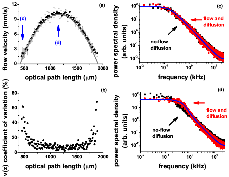
Figure 5 shows results for the dependency of the velocity uncertainty from Gaussian beam waist. Figure 5(a) shows a plot of the beam radius for three focusing lenses measured with a knife edge [17]. The squares correspond to a lens with a focal length of $30$ mm, the circles for a lens with a focal length of $40$ mm, and the triangles for a lens with a focal length of $100$ mm. The dashed lines show the corresponding Gaussian beam models. The measured waist values are $8.5\pm 0.5$ µm, $10.8\pm 0.5$ µm, and $26.3\pm 1$ µm, respectively. Figure 5(b) shows the flow velocity’s coefficient of variation measured in three different experiments with the three lenses. For each experiment the maximum reference flow velocity is $10$ mm/s. As can be observed, the coefficient of variation monotonically decreases for increasing flow velocity for all three lenses. For a particular flow velocity, the choice of a smaller waist results in a lower value for the coefficient of variation compared to the values measured with a larger waist.

Figure 6 shows plots of the power spectral density for an optical path-length near the edge of the channel (Fig. 6 (a)) and for an optical path-length corresponding to the center of the channel (Fig. 6 (b)). The circles show the data and the blue line shows the fitted model. The red line shows only the contribution of the flow term and the green line shows only the contribution of the diffusion term. It can be seen that at optical path-lengths with relatively low flow velocity values the decay of the power spectral density is well described by a Lorentzian (diffusion) decay. However, for relatively larger flow velocities, the decay of the power spectral density at low frequencies is well described by a Gaussian (flow) decay and at high frequencies it converges towards a Lorentzian decay.

Figure 7 shows results for the simultaneous measurement of the diffusion coefficient and the flow velocity based on data similar to the one shown in the previous figure. Figure 7(a) shows the path-length resolved flow velocities for a set of three varying reference velocities. The markers show the measured velocities and the lines show the reference velocities. As can be seen, the measured velocity values are well in agreement with the expected reference values. Figure 7(b) shows the corresponding coefficient of variation for the fitted velocities. For optical path-lengths close to the walls of the channel an increase in the coefficient of variation is observed similar to the case for a fit with fixed diffusion (cf. Fig. 4). Figure 7(c) shows the path-length resolved diffusion coefficient corresponding to the flow velocities shown in Fig. 7(a). The markers show the measured diffusion coefficient and the line shows the diffusion coefficient measured in the no-flow case which have has used here as a reference. As can be observed, the diffusion coefficient measured at relatively low flow velocities is in good agreement with the reference values. For the relatively large flow velocities at the center of the flow channel, a path-length dependency of the measured diffusion coefficient is observed where the diffusion coefficient at the center of the channel is larger than the diffusion coefficient measured near the wall of the channel. As the maximum flow velocity through the center of the channel increases, the overestimation of the diffusion coefficient increases as well. Figure 7(d) shows the coefficient of variation for the fitted diffusion coefficient. For optical path-lengths close to the center of the channel an increase in the coefficient of variation is observed.

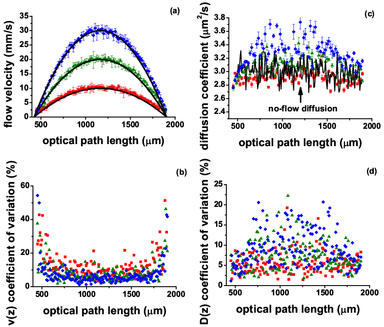
Figure 8 shows results for the simultaneous measurement of the diffusion coefficient and the flow velocity at high flow rates measured with two lenses resulting in a waist of $26.3$ µm and a waist of $10.8$ µm. Figure 8(a) shows the path-length resolved flow velocity and Fig. 8(b) shows the corresponding diffusion coefficient. As can be seen, the flow velocity measured with both lenses and the diffusion coefficient measured with the largest waist are in good agreement with the reference values. However, the diffusion coefficient measured with the smallest waist is overestimated in the center of the channel (cf. Fig. 7). Figure 8(c) and (d) show the coefficient of variation for the measured flow velocity and the diffusion coefficient, respectively. As can be seen, the coefficient of variation for the flow velocity measured with the smallest waist results in a reduced coefficient of variation for the low velocities when compared to the measurement with the largest waist. The coefficient of variation for the diffusion coefficient measured with the largest waist shows a reduced value for the high velocity range when compared to the measurements with the smallest waist.

References

- [1] H. Orihara, Y. Takikawa, “Brownian motion in shear flow: Direct observation of anomalous diffusion,” Physical Review E 84, 061120 (2011).
- [2] R. Weber, R. Rambau, G. Schweiger, K. Lucas, “Analysis of a flowing aerosol by correlation spectroscopy: concentration, aperture, velocity and particle size effects,” Journal of Aerosol Science 24, 485-499 (1993).
- [3] D. Di Carlo, D. Irimia, R.G. Tompkins, M. Toner, “Continuous inertial focusing, ordering, and separation of particles in microchannels,” Proceedings of the National Academy of Sciences of the United States of America 104, 18892-18897 (2007).
- [4] C. Joo, C.L. Evans, T. Stepinac, T. Hasan, J.F. de Boer, “Diffusive and directional intracellular dynamics measured by field-based dynamic light scattering,” Optics Express 18, 2858-2871 (2010).
- [5] K. Drescher, Y. Shen, B.L. Bassler, H.A. Stone, “Biofilm streamers cause catastrophic disruption of flow with consequences for environmental and medical systems,” Proceedings of the National Academy of Sciences 110, 4345-4350 (2013).
- [6] J. Lee, H. Radharishnan, W. Wu, A. Daneshmand, M. Climov, C. Ayata, D.A. Boas, “Quantitative imaging of cerebral blood flow velocity and intracellular motility using dynamic light scattering–optical coherence tomography,” Journal of Cerebral Blood Flow & Metabolism, 33, 819-825 (2013).
- [7] D. Huang, E.A. Swanson, C.P. Lin, J.S. Schuman, W. G. Stinson, W. Chang, M.R. Hee, T. Flotte, K. Gregory, C.A. Puliafito, J.G. Fujimoto, “Optical coherence tomography,” Science 254, 1178-1181 (1991).
- [8] K.K. Bizheva, A.M. Siegel, D.A. Boas, “Path-length-resolved dynamic light scattering in highly random media: The transition to diffusing wave spectroscopy,” Physical Review E 58, 7664-7667 (1998).
- [9] J. Kalkman, R. Sprik, T.G. van Leeuwen, “Path-length-resolved diffusive particle dynamics in spectral-domain optical coherence tomography,” Physical Review Letters 105, 198302 (2010).
- [10] K. Ishii, T. Iwai, H. Xia, “Hydrodynamic measurement of Brownian particles at a liquid-solid interface by low-coherence dynamic light scattering,” Optics Express 18, 7390-7396 (2010).
- [11] R.K. Chhetri , K.A. Kozek, A.C. Johnston-Peck, J.B. Tracy, A.L. Oldenburg, “Imaging three-dimensional rotational diffusion of plasmon resonant gold nanorods using polarization-sensitive optical coherence tomography,” Physical Review E 83, 040903 (2011).
- [12] B.K. Huang, M.A. Choma, “Resolving directional ambiguity in dynamic light scattering-based transverse motion velocimetry in optical coherence tomography,” Optics Letters 39, 521-524 (2014).
- [13] N. Uribe-Patarroyo, M. Villiger, B.E. Bouma, “Quantitative technique for robust and noise-tolerant speed measurements based on speckle decorrelation in optical coherence tomography,” Optics Express 22, 24411-24429 (2014).
- [14] J. Lee, W. Wu, J.Y. Jiang, B. Zhu, D.A. Boas, “Dynamic lights scattering optical coherence tomography,” Optics Express 20, 22262-22277 (2012).
- [15] N. Weiss, T.G. van Leeuwen, J. Kalkman, “Localized measurement of longitudinal and transverse flow velocities in colloidal suspensions using optical coherence tomography,” Physical Review E 88, 042312 (2013).
- [16] H.C. Hendargo, R.P. McNabb, A.H. Dhalla, N. Shepherd, J. A. Izatt, “Doppler velocity limitations spectrometer-based versus swept source optical coherence tomography,” Biomedical Optics Express 2, 2175-2188 (2011).
- [17] A. Arnaud, W.M. Hubbard, G.D. Mandeville, B. de la Clavière, E.A. Franke, J.M. Franke, “Technique for fast measurement of Gaussian laser beam parameters,” Applied Optics 10, 2775-2776 (1971).
- [18] T.W. Taylor and C.M. Sorensen, “Gaussian beam effects on the photon correlation spectrum from a flowing Brownian motion system,” Applied Optics 25, 2421-2426 (1986).
- [19] D.A. Ross, “Focused laser beam effects in optical particle sizing by dynamic light scattering,” Applied Optics 30, 4882-4888 (1991).
- [20] A.J. Pine, D.A. Weitz, P.M. Chaikin, E. Herbolzheimer, “Diffusing-Wave spectroscopy,” Physical Review Letters 60, 1134-1137 (1988).