On the signature of the baryon-dark matter relative velocity in the two and three-point galaxy correlation functions
Abstract
We develop a configuration-space picture of the relative velocity between baryons and dark matter that clearly explains how it can shift the BAO scale in the galaxy-galaxy correlation function. The shift occurs because the relative velocity is non-zero only within the sound horizon and thus adds to the correlation function asymmetrically about the BAO peak. We further show that in configuration space the relative velocity has a localized, distinctive signature in the three-point galaxy correlation function (3PCF). In particular, we find that a multipole decomposition is a favorable way to isolate the relative velocity in the 3PCF, and that there is a strong signature in the multipole for triangles with 2 sides around the BAO scale. Finally, we investigate a further compression of the 3PCF to a function of only one triangle side that preserves the localized nature of the relative velocity signature while also nicely separating linear from non-linear bias. We expect that this scheme will substantially lessen the computational burden of finding the relative velocity in the 3PCF. The relative velocity’s 3PCF signature can be used to correct the shift induced in the galaxy-galaxy correlation function so that no systematic error due to this effect is introduced into the BAO as used for precision cosmology.
1 Introduction
The baryon acoustic oscillation (BAO) method uses the imprint of sound waves in the early Universe on the clustering of galaxies today as a sensitive probe of the Universe’s expansion history (see Weinberg et al. 2013 for a recent review). This in turn constrains the dark energy equation of state, which offers insight into dark energy’s fundamental nature (Albrecht et al. 2006 for a review; Copeland et al. 2006; Li et al. 2011 for model compendia; for recent work on specific models, see e.g. Dutta & Scherrer 2008; Chiba 2009; Chiba et al. 2009; Gott & Slepian 2011; De Boni et al. 2011; Chiba et al. 2013; Slepian et al. 2014). The BAO method’s accuracy depends on precisely modeling how the sound waves frozen in at high redshift imprint on galaxy clustering today, and hence how baryons and DM combine to form these galaxies.
A potentially important effect on early generations of galaxies is the supersonic relative velocity between baryons and DM at decoupling (, recently presented by Tseliakhovich & Hirata (2010). The relative velocity is sourced by the difference in the behavior of baryons and dark matter before decoupling. Prior to decoupling, the baryons and photons form a tightly coupled fluid, locked together by Thomson scattering (linking electrons to photons) and the Coulomb force (linking protons to electrons). This fluid undergoes acoustic oscillations, or sound waves, that propagate to roughly 150 Mpc comoving before halting as electron-photon scattering drops precipitously and decoupling occurs (Peebles & Yu 1970; Sunyaev & Zel’dovich 1970; Bond & Efstathiou 1984, 1987; Holtzmann 1989; Hu & Sugiyama 1996; Eisenstein & Hu 1998). The scale at which these waves halt is termed the sound horizon.
Given an isolated overdense region, baryons nearer to it than the sound horizon are kept in rough hydrostatic equilibrium by the radiation pressure and so do not infall. In contrast, baryons more distant than the sound horizon fall towards the overdensity. Meanwhile, DM on all scales infalls gravitationally. Consequently, the baryons and DM differ in behavior below the sound horizon, resulting in a relative velocity at decoupling on these scales.
It is believed that the relative velocity can modulate the formation of the first galaxies in the Universe on scales similar to the sound horizon (we describe this more below). Since these galaxies are the progenitors of those we observe today, galaxy clustering today may retain a memory of this effect. Yoo et al. (2011) analyze how such a memory might cause a shift in the galaxy-galaxy correlation function by which the sound horizon scale today is measured, an idea also hinted at in Tseliakhovich & Hirata 2010 and Dalal et al. 2010. Given the high precision of current and impending BAO surveys such as BOSS, even a modest, order systematic source of error could significantly bias the inferred cosmological parameters. Therefore it is essential to understand how the relative velocity can induce this shift and how, if the shift is indeed present, it can be corrected. While Yoo et al. (2011) state that the correlation function can shift, their analysis presents results in Fourier space, showing the power spectrum and, importantly, finding that the bispectrum can be used to remove the relative velocity effect from the power spectrum.
Here, we focus on configuration space, for several reasons. First, complicated behavior in the power spectrum and bispectrum often has a simple interpretation in configuration space (Bashinsky & Bertschinger 2001, 2002). Our work shows that the relative velocity is indeed simple in configuration space: it is non-zero only within the sound horizon. Our work therefore makes it clear that any effect on the correlation function is primarily on sub-horizon scales. It is adding or subtracting from the correlation function only inward of the BAO peak that shifts the peak in or out in scale.
Our configuration space approach also offers the new result that, for extracting the relative velocity from the three-point galaxy correlation function (3PCF), Legendre polynomials are an excellent angular basis (Szapudi 2004 and Pan & Szapudi 2005 first suggested such a basis for general measurements of the bispectrum). Because the relative velocity has compact support in configuration space, we can additionally integrate over one side-length of the triangles entering the 3PCF for lengths where the relative velocity has support. This produces a novel compression scheme that improves the chances for detecting the relative velocity in the 3PCF while easing the computational demands of such an effort.
Indeed, this compression scheme is not the only practical advantage of a configuration space approach. The bispectrum is challenging to measure accurately on a cut sky, because survey boundaries break the translational symmetry implicit in a Fourier decomposition. They also impose some miminum wavenumber below which the Fourier representation is truncated, leading to Gibbs phenomenon ringing in the bispectrum. In contrast, in configuration space, the 3PCF can be measured straightforwardly and cut-sky effects corrected by use of an estimator (see e.g. Kayo et al. 2004; Szapudi 2004; Szapudi and Szalay 1998), though at some computational cost (McBride et al. 2011; Marin et al. 2013). Indeed, Pan and Szapudi (2005) have already measured the monopole moment of the 3PCF in Two-degree-Field Galaxy Redshift Survey (2dFGRS), showing the feasibility of this approach.
In the remainder of the Introduction, we give greater detail on the physical mechanisms by which the relative velocity may affect galaxy clustering today: how does the relative velocity effect the first galaxies to form, and how might galaxies today retain a memory of these distant progenitors? The relative velocity affects the formation of early, low-mass haloes, but precisely how remains an open question. In their initial paper presenting the relative velocity, Tseliakhovich & Hirata (2010) predict suppression of halos with due to the relative velocity. Naoz et al. (2012) find this in simulations as well, though simulations by Richardson et al. (2013) find only a small effect in halo number density by . In those halos that do form, the gas content is lowered (Dalal et al. 2010; Tseliakhovich et al. 2011; Fialkov et al. 2012; Naoz et al. 2013). In simulations, Maio et al. (2011) find that star formation in low mass halos is suppressed, though Stacy et al. (2011) argue that the later-time star formation is not strongly affected. The minimum cooling mass for star formation via molecular hydrogen lines also may be raised in simulations (Greif et al. 2011, though Stacy et al.’s earlier work argues it is not). O’Leary and McQuinn (2012) simulate structure formation to show that the relative velocity has a substantial effect on the first mini-halos’ accretion history. Barkana (2013) points out that there may be additional dynamical effects, such as asymmetric disruption of accreting gas filaments and formation of supersonic wakes by halos moving in regions of high relative velocity. Bovy & Dvorkin (2013) suggest that for reasons such as these, star formation in small DM halos may be suppressed enough to resolve the over-prediction of small halos in simulations.
It is believed that the modulation of early, low-mass halos by the relative velocity as discussed above will affect the subsequent formation of the higher-mass halos we observe today, perhaps through feedback channels such as altering the metal abundance or supernovae rate (Yoo et al. 2011). Since these links are not known in detail, it is simply assumed that the relative velocity biases the galaxy overdensity with some amplitude , to be fit from the data. This will be our approach here as well.
Finally, numerous studies have also developed rich small-scale consequences of the relative velocity, though that will not be our focus here. To give only a few examples, Naoz & Narayan (2013) show that the relative velocity modifies the Biermann battery picture of magnetogenesis, while Tanaka et al. (2013), Tanaka & Li (2014), and Latif et al. (2014) consider the impact on primordial supermassive black hole formation. Much work has also investigated the consequences of the relative velocity for the 21 cm radiation field, e.g. Visbal et al. (2012); McQuinn & O’Leary (2012). A detailed recent review of work on the relative velocity is Fialkov (2014).
This paper is structured as follows. In §2, we lay out our approach and assumptions. In §3, we present the structure of the relative velocity due to a point perturbation (the Green’s function), and in §4 we compute the shift the relative velocity induces in the correlation function. §5 discusses this shift and shows how it can be traced back to the compact support of the Green’s function. §6 presents the 3PCF at one vertex of a triangle of galaxies, and §7 connects this with the sum over all vertices that we observe and shows how the 3PCF may be compressed to maximize the signal. §8 concludes. An Appendix presents mathematical results that we use in the paper to accelerate the numerical calculations of §4.
2 Approach and assumptions
We begin by presenting our bias model and then outline how the spatial structure of the relative velocity (which this model requires as an input) can be found using a Green’s function approach.
Throughout this paper, we use linear perturbation theory in configuration space and neglect redshift-space distortions. We model the low-redshift galaxy overdensity, denoted by , as being biased by the square of the relative velocity normalized by its mean value, following Yoo et al. (2011). We then use perturbation theory to compute the correlation function and 3PCF (§4 & §6 respectively).
Writing the relative velocity as (baryon velocity minus dark matter velocity) and (the root mean square value), we define the dimensionless and expand the galaxy overdensity in to ensure . Mathematically, this is
| (1) |
where
| (2) |
captures the standard perturbation theory linear and non-linear bias in the galaxy overdensity.11 1 Often the non-linear bias coefficient is written as (e.g. Yoo et al. 2011; Yoo & Seljak 2013), so care must be exercised in comparing values across different works. in equation (1) is an unknown bias coefficient that, as discussed in , encodes how strongly the relative velocity affects galaxy formation. is the matter overdensity.
We next outline how we compute the spatial structure of the relative velocity, a required input in our bias model (1). Since the true primordial density field at a given location is not known , we need to be able to compute the generated by an arbitrary density field.22 2 We do require linear perturbation theory to be valid, so the field cannot be completely arbitrary. We therefore find the relative velocity due to a point perturbation and then integrate it against the true density field. Though this latter is not known , its statistical properties are. As we will only be considering expectation values over , and thus over the density field, this is sufficient.
Since the response to an impulse is called the Green’s function, we denote the relative velocity due to a point perturbation by . By symmetry, it must always point radially outward from the density point sourcing it. It points outward because DM infalls under gravity and baryons are static or pushed outwards by radiation pressure.
We now define the Green’s function implicitly:
| (3) |
To linear order, the relative velocity at redshift due to a primordial density field is found by integrating against the Green’s function. Isotropy demands that . Notice that represents the dipole moment of the density field weighted by , suggesting that multipole expansions will be natural moving forwards. Figure 1 portrays schematically the use of the Green’s function to compute the relative velocity (and its square) due to an arbitary density field.
The Green’s function formalism above makes it evident that in our bias model, the square of the relative velocity contributes to the correlation function only beginning at fourth order in the perturbed quantities. One overdensity is required to source a relative velocity field, as shown in the lefthand panel of Figure 1, and to produce (equivalently, two overdensities are needed, as shown in the righthand panel of Figure 1. For a Gaussian random field, all odd moments vanish, meaning the velocity contributes to the correlation function beginning only at fourth order. To obtain all of the fourth order contributions to the correlation function, we must expand to second order in equation (2):
| (4) |
Here and throughout, is the linear density field while is the second-order density field, which is .


Finally, we close this section with four further points about our perturbation theory framework. First, we note a subtlety of our bias model. and so if we carried through the expansion of the galaxy overdensity to higher orders in we would expect these terms to contribute to the correlation function at order unity times some combinatoric factor. For instance, in the limit that (a 3-D Dirac delta function) one can compute explicitly that a term appears in if equation (1) is taken out to . Since there are potentially an arbitrary number of these terms, one might ask if our expansion converges.
However, physically, it is likely that the dimensionless parameter of importance for galaxy formation is where is some unknown, redshift-dependent circular velocity or velocity dispersion for a typical galaxy. We expect that so that an expansion in powers of this quantity would converge. Our expansion, now with the coefficient of labeled by , may be rewritten in terms of by taking
| (5) |
The are coefficients of an expansion in terms of powers of and are assumed to be all intrinsically on the same order of magnitude. Solving for shows that it must fall rapidly with and our expansion converges.
Second, we justify the use of linear perturbation theory. Though perturbation theory does not provide highly accurate fits to simulation results on small scales (), the large scales () relevant for the BAO have remained roughly linear down to the present day (for discussion of non-linear effects, see Smith et al. 2003; Seo et al. 2008; Sherwin & Zaldarriaga 2012, though see also Roukema et al. 2014). The primary effect of what non-linear evolution has occurred is to broaden the BAO peak in the galaxy-galaxy correlation function, not to shift its center. As Eisenstein et al. (2007a) show, the peak position is robust in configuration space. Further, modern BAO surveys (e.g. Anderson et al. 2014) use reconstruction to compute the peculiar velocity field implied by a given density field and reverse it, thus allowing analysis to be performed on a density field that is linear to even better approximation (Eisenstein et al. 2007b; Seo et al. 2008). These considerations justify our use of linear perturbation theory to compute how the relative velocity effect shifts the BAO peak. It is unambiguous to calculate the lowest order change in the correlation function and 3PCF the velocity produces. As we discuss above, higher order corrections should quickly become negligible. One can debate the precise details of the no-velocity correlation function, but the addition from the velocity to any model chosen can be accurately computed in perturbation theory.
Third, when computing the expansion of the density field to second order, we only consider effects generated by gravity. For example, we neglect effects due to couplings of radiation and matter. Naoz & Barkana (2005) point out that on small scales, the sound speed varies spatially after recombination due to density-dependent Compton heating (see also Naoz et al. (2011)). This will not affect our conclusions because the BAO scale is dominated by the relativistic sound speed prior to decoupling. Another effect generated by coupling of radiation and matter is the impact of inhomogeneities in the intergalactic medium on the Lyman- emission observed from galaxies (Wyithe & Djikstra 2011). This can create an additional clustering signal on large scales that would need to be properly accounted for if one wished to use the techniques in this work on a Lyman- selected galaxy sample such as might be found using the Hobby-Eberly Telescope Dark Energy Experiment (HETDEX).
Finally, we consider the effects of redshift-space distortions (see Hamilton 1998 for a review). Peculiar velocities systematically alter galaxy clustering even on large scales (Kaiser 1987; Bernardeau et al. 2002), introducing a strong directional dependence. These distortions do not substantially alter the Green’s function picture, because galaxy positions in redshift space are shifted by much less than the acoustic scale. However, the distortions can alter the resulting correlations because the true large-scale correlations are also small. These effects can be accurately treated in cosmological simulations, and we expect that studies of observational data would want to compare to full simulations. However, we note that our analysis will average over triangles irrespective of their orientation to the line of sight. While not optimal as regards information content, such averages do tend to reduce the effects of redshift distortions on large scales. For example, the redshift-space spherically averaged two-point correlation function on large scales is primarily a rescaling of the real-space result, with a mild extra broadening of the acoustic peak. We similarly expect that our orientation-averaged 3PCF results will be only mildly changed by redshift-space distortions. Furthermore, the reconstruction of the linear density field discussed above can also correct redshift-space distortions on the scales relevant for this work by introducing a factor , where , is the linear growth function, and is the scale factor. This factor represents the additional squashing along the line-of-sight (Eisenstein et al. 2007b). This technique should allow removal of the redshift-space distortions on the large scales most significant for the signature presented here.
3 Deriving the Green’s function
We now seek to obtain an explicit expression for the Green’s function. We begin with the linear theory continuity equation in configuration space. is the scale factor and we use comoving positions and velocities. An overdot denotes a derivative with respect to time. We have
| (6) |
which Fourier transforms to
| (7) |
where a tilde denotes a 3-D Fourier transform given by
| (8) |
with inverse transform
| (9) |
For growing modes, is parallel to so
| (10) |
This means
| (11) |
where subscript c is for CDM, b for baryons, vbc for relative velocity, and we define the relative velocity transfer function
| (12) |
and are the baryon and CDM transfer functions, which give the evolution of each mode with redshift via
| (13) |
is the primordial density perturbation related to the primordial power spectrum by , with .33 3 is fixed by the value of today. We emphasize that the relative velocity transfer function maps the primordial density field to a velocity field at some redshift so always acts on .
We now obtain the configuration space Green’s function, defined implicitly by equation (3). Using the Fourier representation of (11) we have
| (14) | ||||
We then rewrite to find
| (15) | ||||
Changing variables on the left-hand side via and then equating the resulting integrands over , we have
| (16) |
which, projecting onto , results in
| (17) | ||||
Above, and is the spherical Bessel function of order one. We now have the desired velocity Green’s function. Noting that its Fourier transform is closely related to the velocity transfer function, for notational consistency we define
| (18) |
and use going forward.
In practice, we compute by transforming using equation (17). Thus we must first compute . Using a flat cosmology with , , , and , we output transfer functions and from CAMB (Lewis 2000) on a grid equally spaced in with 5,000 divisions per decade from to . To approximate and (cf. equation (12)), we discretize the derivative at each redshift with . To avoid ringing due to the finiteness of our grid in Fourier space, we use a smoothing to evaluate the integral (17) (and all analogous integrals over in what follows).
Figure 2 shows the Green’s functions for and at . We have multiplied each by for two reasons. First, for a random distribution of densities, a spherical shell of radius will contribute as when integrated over volume. Second, this weighting renders the fine structure more apparent. The most striking feature of Figure 2 is the compact support of the Green’s function. This occurs because for , , as radiation pressure cannot support the baryons against gravitational infall. Also salient is that for : baryons are in hydrostatic equilibrium with . There is a bump in the baryon velocity at due to the outgoing baryon-photon overdensity from the BAO. Meanwhile, the DM infalls.
Inside the DM infalls as roughly rather than because the baryon-photon fluid’s contribution to the potential, which, during radiation domination, overshadows that of the DM overdensity at the origin, is diluted. For a test particle at , some of the baryon-photon overdensity is outside a Gaussian sphere of radius , and hence does not contribute to the gravitational force felt by the particle. This is equivalent to the fact that modes inside the horizon grow less quickly than those outside the horizon during radiation domination, and is why the DM transfer function turns over for the wavenumber entering the horizon at matter-radiation equality. Using the continuity equation in Fourier space (equation (7)), slower growth of a given mode implies a lower velocity field for that mode, so modes inside the horizon indeed have a lower velocity field than those outside the horizon.

4 Analysis of the two-point correlation function
4.1 The shift in
We now wish to compute , the relative velocity contribution to the correlation function. We define as the full galaxy-galaxy correlation function including and denote the late-time linear matter correlation function . To compute , we use the galaxy overdensity bias model of . Numerical subscripts denote spatial positions: . For more compact notation, we also define ; note this is second-order in . We have the velocity contributions to the product :
| (19) | ||||
Defining and noting that terms in vanish because we assume a Gaussian random field, we have
| (20) | ||||
The factors of 2 come from invoking homogeneity so that and Moving forward we will often denote the term proportional to by and analogously for the terms in and , as indicated above. We have also dropped terms above fourth order.
Using the definition of , we can simplify the three terms in to:
| (21) |
| (22) |
| (23) |
For equation (22), we have replaced by . These three terms (ignoring the constant offsets) are shown schematically in Figure 3. Spheres indicate a velocity squared, while the solid square shows the density field squared and the solid triangle represents the second-order density field . The dotted lines show the correlations that remain after the constants above are subtracted off.
Note that these expectation values involve products of four values of the linear density field at different locations. Since the linear density field is a Gaussian Random Field, we can use Wick’s theorem to simplify. The constants subtracted above are just generated by the presence of in our model for , and ultimately cancel when Wick’s theorem is applied.
Finally, we need to compute since it enters equations (21)-(23). We have
| (24) | ||||
with given by equation (17). See the right panel of Figure 1 for a visual reminder of how is calculated from the Green’s function. For , we in turn require , which can be found by writing in the Fourier basis using equations (14) and (15), squaring, and taking expectation values. One then uses the relation between and given in §3 to simplify the integrals and finds
| (25) |
in agreement with Dalal et al. (2010).
Note that after decoupling, the relative velocity is no longer sourced and will therefore decay as , as will Hence after decoupling is redshift-independent.


4.2 as convolutions
We now show that can be expressed as convolutions of various functions of the linear density field with a 6-dimensional velocity kernel we define below. This latter preserves the radial structure of the Green’s function, and this insight will support our analysis in §5 of why the BAO peak shifts.
We begin with (equation (22)) because it is the simplest. The disconnected part of is and so cancels off. Focusing on the remaining terms from Wick’s theorem, represented by the dotted lines in Figure 3, we find
| (26) |
where the factor of relative to equation (22) comes from Wick’s theorem. To connect with Figure 3, note that we have put the origin at the black dot (i.e. used homogeneity to set in equation (22)). We have defined the 6-dimensional velocity kernel
| (27) |
This kernel generates from integrals over and for all and within roughly of the origin. Note that it is redshift-independent. We have also defined : a heterosynchronous correlation of the low-redshift linear theory matter density field with the primordial density field:
| (28) |
where
| (29) |
The matter transfer function is . Note that is not the standard power spectrum, which would use the square of the transfer function. Rather, is is a cross power spectrum between the low-redshift linear theory matter field (we use ) and the primordial density field.
We define the 6-D convolution as
| (30) |
where is a 6-D vector and and are 3-D vectors. With this definition, it is immediate to write
| (31) |
We now show that (equation (23)) can also be expressed as a convolution. Canceling the disconnected part and then evaluating (see Figure 3), we find
| (32) |
where again the factor of relative to equation (23) is from Wick’s theorem. Note that for we are correlating a velocity field with a velocity field, and so we must use only , leading to in the expression above. Let us first consider the integrals over above. Flipping the signs of and which leaves the Jacobian unchanged, and applying the definition (30), we obtain
| (33) |
Inserting this in equation (32), we have
| (34) |
Applying again the definition (30), we find
| (35) |
Finally, we turn to (equation (21)), the most difficult term to evaluate because it involves the second-order density field . Using the same procedure as for and , we have
| (36) |
where the factor of relative to equation (21) is again from Wick’s theorem. Again, Figure 3 illustrates the relevant correlations. is the Fourier transform of the second-order kernel
| (37) | ||||
(Goroff et al. 1986; Jain & Bertschinger 1994; Bernardeau et al. 2002 [equation (45)]). Analogously to , an integral of two density fields and against generates a second-order density field . The s are Legendre polynomials.
Working now in Fourier space, we see that equation (36) becomes
| (38) | ||||
Note that the integral over in equation (36) is the 6-D convolution , which we have rewritten as a product in Fourier space using the Convolution Theorem to obtain equation (38). In equation (38), the integral in square brackets becomes a function of and when evaluated; this in turn is convolved with . For convenience, we define the integral in square brackets as
| (39) | ||||
It is more convenient to work with this representation than to directly consider , since (the Fourier transform of ) is divergent without the regularization multiplication of by the smoothed cross power spectrum provides. With this notation, we now have
| (40) |
Thus, from equations (31), (35), and (40), we see that all three terms in are just convolutions of various functions built from the correlation function with the 6-D velocity kernel (27) we have defined. This latter ultimately encodes the radial structure of the Green’s function, shown in Figure 2.
We now pause to examine the limit that , as this will offer strong physical intuition for the behavior we should see once we have numerically evaluated the equations above. In this limit, , while (unfortunately is divergent in this limit).
The approximate form that for (see Figure 2) means that inside each radial bin of volume will give an equal contribution to . We thus expect that will be approximately a step function, constant for and zero otherwise. Meanwhile, is an autocorrelation, so will peak at A second, lesser peak in the autocorrelation occurs at , which becomes the most prominent one when we consider the volume-weighted . Therefore should have a well-defined peak that encodes the acoustic scale, and have support out to . These behaviors are displayed in the lower panel of Figure 5, magenta dashed and orange X-ed curves.
4.3 Evaluating the convolutions
We now give details on how the convolutions of the previous section can be quickly evaluated. Formally, the convolutions are multidimensional integrals, and so could be computed directly via Monte Carlo methods. We avoid this by showing that in principle all of the convolutions can be analytically reduced to one-dimensional radial integrals, because the angular dependences of all functions involved are known. This is highly desirable and may be done using results we prove in the Appendix.
First, we explicitly obtain ; since this is also useful in computing the 3PCF, we write it down here. We have
| (41) | ||||
where the , defined in the Appendix (equations (61) and (62)), are 2-D transforms composed of 1-D integrals against spherical Bessel functions (these latter integrals are closely related to Hankel transforms). Simplifying (see Appendix for formulae used to do so), we have
| (42) | ||||
with
| (43) |
and
| (44) |
This reduces the terms in to
| (45) | ||||
| (46) |
and
| (47) | ||||
Note that the right-hand side of each equation is a function of , as and (equations (18) and (29)) are functions of , and the s bring them to functions of (cf. equation (62)). The equations above allow efficient numerical evaluation of . Finally, it should be noted that Wick’s theorem yields immediately that (cf. equation (23)). Taking this limit of equation (47) explicitly cross-checks our use of the convolutional formalism:
| (48) |
with the last equality using equation (25).
5 Explaining the BAO peak shift
We begin with a descriptive sketch of why the BAO peak shifts and then move to more detailed discussion of our numerical results. First: the key aspect of that allows it to shift the BAO peak in the correlation function is the sharp drop to zero for greater than roughly . This can be traced back to the same feature in the relative velocity Green’s function (see Figure 2). Thus adds or subtracts probability density from asymmetrically, doing so primarily inwards of . It is this asymmetric alteration that pulls the BAO peak in or out in scale. Fundamentally, then, the shift is due to the presence of an acoustic horizon: the relative velocity is at root a pressure effect, and as such can alter correlations roughly only within the sound horizon.
In greater mathematical detail, the 6-D velocity kernel has support only for . Convolving and with it act as smoothing operations that simply broaden its peak. Since the smoothing functions are so narrow, the convolutions are only non-zero essentially where the velocity kernel is non-zero. For this adds probability density inwards of , while for , this subtracts probability density inwards of . Figure 4 shows the two smoothing functions, and (built on transforms of ), and the Green’s function they smooth. The behavior of the contribution from is complex, as it is a double convolution, but as we learned from the limit, it has support out to . However, around the BAO peak location is roughly symmetric, so it does not contribute much to shifting the peak (Figure 5).
We now move to discuss each term in more extensively; each term is shown in Figure 5. Two of the terms are fairly simple in structure, and can be understood by recalling the limit of §4.2. is roughly constant for , and drops quickly to zero outside the sound horizon. It extends slightly beyond the sound horizon; this may be traced back to the smooth drop of the velocity Green’s function (Figure 2) produced by the neutrinos and Silk damping. The small bump near the sound horizon is due to the baryons’ velocity there; this has its origin in the baryon velocity’s contribution to the Green’s function (see Figure 2). This is confirmed by the bottom panel of Figure 5, plotting the limit. Here, a bump is still present near the acoustic scale, meaning that the bump is due to structure in the velocity Green’s function and not due to any structure in . Since is non-zero essentially solely inside , it adds asymmetrically to the correlation function and hence can pull the BAO bump inwards () or outwards ().
is also fairly simple and can also be understood by recalling the limit of §4.2. From equation (35), we see that it is a double convolution, and that the first convolution produces a function identical, up to amplitude, to . However, this is then convolved with an additional velocity kernel, which is, unlike and , rather broad. Thus there is overlap between the velocity kernel and the first convolution until nearly twice the sound horizon. However, is roughly symmetric around the acoustic scale out to on either side of it; this means that in the region of the BAO peak, is adding symmetrically to and hence will contribute minimally to shifting the peak.
We now discuss the last remaining term in , . This term has the most complicated structure, a consequence of its generation by the second-order density field. This latter is non-local: computing requires integrating over all space (see Figure 3, top panel, and equation (36)). Hence this term requires correlating the entire linear density field with the velocity field. Nonetheless, its behavior can be understood qualitatively. The second-order density field (or the kernel) represents non-linear gravitational evolution, which, in our Green’s function approach, pulls mass towards the origin. Thus it is not surprising that is rather narrow. Since is so narrow, it will only have non-zero overlap with where the latter is non-zero. This explains the compact support of . is able to become negative because does. Note that (Figure 4) is positive very close to the origin; this is what permits to become positive at intermediate scales, . Overall, for , mostly adds to inwards of the BAO bump and subtracts from it directly outside the sound horizon; this asymmetric effect can shift the BAO peak.
In summary, then, we have seen that of the three terms entering , only two make significant contributions to a peak shift. In both cases, the shift is due to the compact support of these terms, which in turn results from the narrowness of the smoothing functions combined with the compact support of the velocity Green’s function. We now consider the relative importance of these two terms when they are added together with plausible values of the linear and non-linear bias. Note that both of these terms are proportional to , so different values of will not alter their relative weights. is a factor of larger than , and so it dominates the total velocity contribution to for . The total velocity contribution to in Figure 6 thus looks very similar to . Note however that the effects of are perceptible. In particular, inside , the addition for is greater in magnitude than that for . This is because for and are both mostly positive within , while for , flips sign but does not (compare and curves in Figure 6). Outside , the case is reversed. For , as is , while for , these two terms have opposite signs and thus interfere destructively. This point explains why the curve for is larger in magnitude than that for outside . Finally, the convergence of the curves to those with at large is because the term is the only contribution for and it is symmetric in . Note also that the curves are nearly anti-symmetric under sign flip in , not surprising since two of the terms manifestly have this symmetry. They are not perfectly anti-symmetric under this transformation due to the term.
It is significant that the term dominates the velocity addition to because this means one need not measure as well as one measures to obtain a good correction to the correlation function. Fortunately observationally is indeed measured better than .


6 Isolating from the 3PCF: pre-cyclic computation
The three-point galaxy correlation function (3PCF) describes the excess probability over random of finding three galaxies with positions , , and ; that is, in a given triangle configuration. We compute it at fourth order using our bias model ((1), (2), and (4)) as
| (49) | ||||
We now rewrite the pre-cyclic piece (subscript “pc”) as a function of two side lengths and their enclosed angle (so that numerical subscripts denote sides of the triangle rather than spatial positions):
| (50) | ||||
Here, the phrase “pre-cyclic” means that we choose one vertex of the triangle of galaxies at which to define and the two sides enclosing it, and . Note that in the product of three copies of needed to form the 3PCF, each of the three galaxies can contribute a a and a . The pre-cyclic term is written by choosing one galaxy to contribute each of these (it may be the same one). We have chosen the third galaxy to contribute all of these more complicated terms. Since we can then take this galaxy to be at the origin, this approach simplifies the calculation. However, to connect with observations, where there is no “preferred” vertex (galaxy), we eventually must sum cyclically, giving each galaxy in the survey the chance to contribute and . This procedure and its results are described in §7.
We now may calculate explicitly from perturbation theory.44 4 Notice that , and (equations (40), (31), and (35)) are in fact just convolutions of with the three terms of . Unfortunately, the weights with which these convolutions enter (respectively , , and ) differ from those with which the three terms of enter (equal weights), so is not quite the convolution of with . Motivated by the fact that is a weighted dipole moment of the density field, we expand the angular dependence of using Legendre polynomials as a basis.55 5 In the more general context of discussing a new set of estimators for 3-point statistics, many years before the discovery of the relative velocity effect, Szapudi (2004) suggested decomposing the bispectrum’s angular dependence in Legendre polynomials. Our work here differs because we are interested in the configuration-space behavior as it is there that the acoustic structure of the relative velocity will be distinctive. Importantly, subsequent work of Pan and Szapudi (2005) exploits this basis in configuration space (a measurement of the monopole moment of the 3PCF in 2dFGRS), illustrating the utility of this decomposition in both Fourier and configuration space. We find
| (51) |
with the coefficients as
| (52) |
| (53) | ||||
and
| (54) |
is the linear theory matter correlation function at ; and are defined analogously to the earlier and (equations (43) and (44)) as:
| (55) |
and
| (56) |
Recall that numerical subscripts on and indicate spatial position. Factors of 2 enter all terms above (e.g. ) due to Wick’s theorem, which reduces the four linear fields implict in each expectation value of equation (50) to a sum of products of three expectation values over two linear fields each, one of which cancels off due to the subtractions in equation (50). The two that remain are the same by homogeneity. The coefficients, in equation (52), in equation (53), and in equation (54) can be traced back to equation (37) for the kernel generating the second-order density field, multiplied by the from Wick’s theorem. The negative sign in equation (53) relative to this kernel is because the term in equation (53) comes from a Legendre polynomial of odd order in equation (37) and so picks up a factor of when transformed according to equation (60).
The functions appearing in the pre-cyclic term, and the products of these functions evaluated on isosceles triangles, are shown in Figure 7. In both plots the structure around should particularly be noted, as it is ultimately why the 3PCF will have signatures of both the standard BAO and the relative velocity. Finally, in the pre-cyclic 3PCF, enters only at , the dipole term. Given that it is this term that generates in the first place, this result is not surprising.


Figure 8 shows the behavior of the coefficients that enter into the Legendre polynomial expansion of the pre-cyclic term at (equation (53)), the relevant multipole for the velocity. receives an increment from the velocity for roughly isosceles triangles with two sides of length This can also be seen in the bottom panel fo Figure 7, which is a trace along the diagonals of the three panels in Figure 8. The relative velocity effect also produces a very modest decrement for triangles with one side of length and one side of length . The part of due to the usual (no relative velocity) terms also has acoustic structure, with an increment for triangles with one or more side of length . Adding the velocity (for ) and non-velocity contibutions to together produces a sharp increment for isosceles triangles with two side lengths , while the decrement from the relative velocity for triangles with one side is so modest as to be washed out by the no-velocity contribution.


7 Isolating from the 3PCF: cyclic summing and compression
In §6, we discussed the effect of the relative velocity on the 3PCF with the simplification that we had chosen to evaluate and at the origin. This corresponds to our knowing which galaxy is contributing these terms to the 3PCF; in practice, we do not know this. Therefore, to give each of the three galaxies in a given triplet a chance to contribute these terms, we must cyclically sum the pre-cyclic 3PCF equation (50) around the triangle specified by and We verify our prescription for this sum by calculating the reduced 3PCF in a power-law case and comparing with Bernardeau et al. (2002)’s result (their equation (159) and Figure 10). After cyclically summing, we re-project onto the basis of Legendre polynomials to find the radial coefficients for a multipole expansion of our 3PCF (the analog of equation (51)). These are
| (57) | ||||
with . Note that and are all functions of and , easily found using the law of cosines. The factor of is necessary because ; that is, the Legendre polynomials are an orthogonal but not orthonormal basis. Where in the pre-cyclic terms, we only found terms up to , cyclically summing introduces higher orders. Indeed, generically the cyclic sum projects onto an arbitrary number of Legendre polynomials. We present the first few modes, split by bias coefficient, in Figure 9.
In Figure 9 we must apply a more complicated weighting than our usual weighting to the 3PCF. The 3PCF projections become very large in magnitude for isosceles triangles. This is because when , the Legendre polynomial being projected onto becomes very large. This heavily weights squeezed triangles with zero opening angle. When these triangles are also isosceles, their third side is zero, causing rapid increase in the functions of side length entering the pre-cyclic terms as these functions go roughly as . These triangles are precisely those we must exclude, since for one side length we expect perturbation theory to be invalid. We have therefore suppressed the diagonal by multiplying by a Gaussian weighting .66 6 Several choices of width for the Gaussian weighting were considered before choosing as the best numerical factor above. We also weight by to make the fine structure more apparent and to capture the expected contribution of each spherical shell with volume .
As we might expect, the velocity signature is strongest in but has echoes in and additional structure in In particular, the velocity bias produces in an increment for triangles with two sides and a decrement for triangles with one side and one side . This is consistent with what we might expect from the pre-cyclic term, which also has an increment and decrement for these respective configurations. Indeed, this can be roughly interpreted as a blurring of the structure present in the pre-cyclic velocity plot (compare Figure 8, bottom panel, with the , panel in Figure 9). Neither of the other bias coefficients contribute such an effect to . The velocity bias produces in a decrement for triangles with one side and one side . Neither of the other bias coefficients contribute such an effect to . The results for and are very similar to those for . This is because the higher-order Legendre polynomials are more sharply peaked at , and so the triangles with (zero opening angle) and are weighted heavily.77 7 One can see this by noting that around the s have series expansion and so the drop in weight as decreases from 1 is more severe for higher . Thus as for large , the same small subset of triangles is dominating the projection integral (57), meaning the projections will be similar for and .
The 3PCF decomposition we have presented thus far has two independent variables: the two triangle sides and . It is worthwhile to consider whether this information can be compressed into a function of one independent variable. By reducing the dimensionality of the problem, such a compression would ease handling of the covariance matrix associated with an eventual measurement, for example by accelerating the computations required in analyzing a large number of mock catalogs. Further, a clever compression might allow us to avoid entirely the squeezed limit (isosceles triangles with small opening angle so that the third side approaches zero), in which perturbation theory is not expected to be valid because two of the galaxies are very close to each other. Finally, a compression might allow us to focus on the set of triangles where the relative velocity is most pronounced: as Figure 9 and our previous discussion indicate, the relative velocity is localized to specific triangles in all . In particular, on the scales expected to be better controlled observationally (i.e. those with and ), the relative velocity is in a fairly condensed region of the multipole.
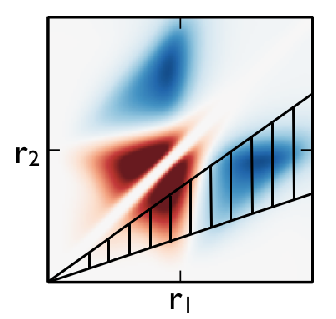
With these desiderata in mind, we integrate the 3PCF’s multipole moments (displayed with weighting in Figure 9) over one triangle side, but constrain this side to be within some fraction of the side that remains a free variable. We term this approach “compression.” If we integrate over and constrain , we can avoid any triangle side’s nearing zero. The minimum of will be , and by the Triangle Inequality the minimum of the third side, , will be . Thus all three triangle sides remain sufficiently large that perturbation theory should be valid. This compression scheme is shown in two different ways in Figure 10; the top panel portrays its effect in configuration space, while the bottom panel shows the region of each panel in Figure 9 integrated over. Notice that the region of integraton captures much of the area where the relative velocity is important in . Several intervals for were considered before choosing ; in an observational study the exact interval chosen might differ as optimality will somewhat depend on the signal-to-noise at different scales, an issue we do not treat in detail here.
Summarizing mathematically, to obtain the compressions at each split out by bias coefficient, denoted and , we compute
| (58) |
where ranges over and is the volume of the shell being integrated over.
Figure 11 shows that each we study can be used to detect the relative velocity effect, with the strongest constraint coming from as might be expected given that this is the only mode where the velocity contributes in the pre-cyclic 3PCF. It is encouraging that through even show differences between the effect and no-effect models at scales as this smaller side length increases the number of triangles available in a given survey volume relative to triangles with side length where the effect is most pronounced in . Interestingly, the effect in all ’s studied at scales is substantial, though survey volume limitations may not permit strong constraints to be derived from such large scales. We have weighted the compressions by to display the finer structure as well as to simulate shot noise-limited measurements. Shot noise is inversely proportional to , the number of galaxies in a given spherical shell, so it scales as . Meanwhile the signal is proportional to the number of galaxies, so .
8 Discussion and conclusions
Previous work by Yoo et al. (2011) has argued that the relative velocity effect can shift the scale at which the BAO peak appears in the galaxy correlation function . In this work, we have shown that the relative velocity’s shift to is generated because the relative velocity itself is non-zero only within the sound horizon at decoupling (Figure 2). More precisely, we have explicitly calculated that the velocity corrections to the correlation function are all generated by convolving relatively narrow functions with a kernel that shares the radial structure of the velocity Green’s function. Hence the spatial structure, in particular the compact support, of the Green’s function is inherited by the velocity corrections to . Thus, these corrections can alter the correlation function only below roughly the sound horizon.88 8 has support out to , but since this term scales as it is less important than and , which drop nearly to zero outside . Adding or subtracting from the correlation function only below this scale can change the radius at which the BAO peak occurs; a negative velocity bias pushes it outwards while a positive bias pulls it inwards.
To correct this shift and ensure that the BAO remain an accurate cosmological ruler, the relative velocity bias must be measured. Motivated by the previous work in Fourier space of Yoo et al. (2011), we have presented a configuration-space template for fitting the three-point function to isolate We have shown that the full 3PCF has robust radial signatures of the relative velocity effect that are unique and cannot come from any other bias term at the order in perturbation theory to which we work, in agreement with Yoo et al. (2011). Furthermore, we have offered a useful basis for measuring the full 3PCF and then suggested a further scheme for processing these results. This scheme should unambiguously expose the relative velocity’s signature while avoiding the regimes in which perturbation theory is expected to be inadequate. It will also likely ease handling of the covariance matrix if large numbers of mock catalogs are to be used for computing error bars.
Previous attempts to constrain the relative velocity observationally have focused on Fourier space. We have already alluded to the advantages of configuration space in §1, and we revisit these points here. On the theory side, our configuration space approach has exposed the relatively simple spatial structure of the relative velocity. Fourier-space work on the bispectrum does not render transparent which triangle configurations are optimal for velocity bias constraints. Our configuration space approach immediately shows that, on scales small enough to measure with current surveys, the velocity signature is localized to a small region of triangle side lengths and a single multipole (). This localized signature (see Figure 9) naturally suggests that an integral over the desirable region would enhance the velocity signal-to-noise, an intuition borne out by our compression scheme results (Figure 11), which, it should be noted, are weighted to reflect shot noise.
On the practical side, there are also considerable advantages to working in configuration space. As we have already discussed in §1, edge-correction is much simpler in configuration space. Further, Pan & Szapudi’s (2005) measurement of the monopole moment of the 3PCF shows it is possible in practice to extract information from a multipole decomposition of the 3PCF. Looking forward, in forthcoming work we will present a fast algorithm for computing the multipole moments of the 3PCF while accounting for edge correction. This work will also address in more detail the covariance matrix of the 3PCF.
Thus far, the bispectrum technique of Yoo et al. (2011) has not been used to constrain the relative velocity. Therefore three-point statistics remain an entirely unexploited means of gaining traction on the relative velocity, a situation we hope the configuration space signatures of this work will improve. Nonetheless, recent work by Yoo & Seljak (2013) has used measurements of the power spectrum in the Constant Mass (CMASS) sample of the Sloan Digital Sky Survey (SDSS) DR9 (260,000 galaxies) to compute a root-mean square shift of in the BAO peak position, showing this shift can potentially be of order the entire error budget for the BAO distance measurement. It should be noted that Yoo & Seljak’s best-fit parameter values imply no relative velocity at all (the root-mean square shift is from integrating over the probability distribution of the linear, non-linear, and velocity biases). On the other hand, a velocity bias of as large as (in our units; they use different values of and from our fiducial case so must be rescaled for comparison) is consistent with their measurement at one sigma.99 9 They find , so we rescale such that . Their definition of differs from ours by a factor of and is having accounted for this. This has also been done where we quote in the best-fit case from their work.
A limiting factor in their analysis is the growth of the error bars at smaller wavenumber (large scales; see their Figure 6); as our analysis shows (see our Figure 6), large scales are important for the relative velocity’s addition to the correlation function. In this context two points should be made. First, even when restricted to measurements of the power spectrum (or correlation function), controlling the error bars on large scales should have significant rewards, meaning increasing the number of galaxies used for the measurement is highly desirable. Thus use of the full sample of million galaxies in the most recent SDSS data should offer compelling new constraints. Second, the distinctiveness of the 3PCF signature, where obtaining the dipole moment already begins to isolate the velocity signature, should render the large-scale error bars less problematic even at fixed number of galaxies.
Finally, a separate issue our work clarifies is how to constrain the non-linear bias. Our compressions show that the higher multipoles are extremely insensitive to the non-linear bias, while for and it contributes much more strongly than the linear bias for a given magnitude of both (see Figure 12). Given that the non-linear bias enters only at in our pre-cyclic calculation (equation (52)), we indeed expect its projection onto and close-by multipoles to be strongest. This suggests that measuring different multipoles of the 3PCF, compressed as we outline, should offer a robust way to separate the linear bias from the non-linear bias. As the Yoo & Seljak (2013) best-fit measurement from CMASS shows, the non-linear bias may be in our units (their Figure 6), in which case Figure 11 shows it would contribute of what the linear bias does at scales in but negligibly in and up. We hope the compression scheme presented here will, independent of its utility for relative velocity measurements, provide a new method to extract the non-linear bias from 3PCF measurements.
Robustly separating the non-linear bias from other effects may also prove helpful in correcting the BAO peak shift if one is found. Yoo & Seljak (2013) find that non-linear bias can also shift the BAO peak. Historically has been constrained using the 3PCF or bispectrum (Scoccimarro et al. 2001; Verde et al. 2002; Wang et al. 2004; Gaztañaga et al. 2005; Gaztañaga et al. 2009; McBride et al. 2011b; Marin 2011; Marin et al. 2013; Guo et al. 2014), and our compressions offer a particularly clear way to isolate from the linear bias and from the velocity bias . This separation should aid accurate measurements of both and and ensure the peak shift can be corrected.
With the percent-level constraints on the cosmic distance scale the BAO method offers through surveys such as BOSS (Anderson et al. 2014) and the concomitant limits on dark energy’s equation of state (Aubourg et al. 2014), understanding any sources of bias is essential. In future work, we will implement the strategy discussed here to measure using data from SDSS-III and assess whether the imprint of the relative velocity between baryons and dark matter might be present at a level relevant to modern BAO surveys.




Acknowledgements
ZS thanks Neta Bahcall, Jo Bovy, Pierre Christian, Cora Dvorkin, Anastasia Fialkov, Doug Finkbeiner, Margaret Geller, JR Gott III, Laura Kulowski, Avi Loeb, Chung-Pei Ma, Robert Marsland, Cameron McBride, Philip Mocz, Jim Moran, Stephen Portillo, Matthew Reece, Mohammadtaher Safarzadeh, David Spergel, and Harvey Tananbaum for useful discussions during this work. ZS especially thanks Harry Desmond, Meredith MacGregor, Smadar Naoz, Yuan-Sen Ting, and Anjali Tripathi for comments on the manuscript. We also thank the anonymous referee for comments that considerably improved the scientific content and presentation of this work. This material is based upon work supported by the National Science Foundation Graduate Research Fellowship under Grant No. DGE-1144152.
References
Adams JC, 1878, Proceedings of the Royal Society of London, 27, 63-71.
Albrecht A et al., 2006, Report of the Dark Energy Task Force, preprint (astro-ph/0609591).
Anderson L et al., 2014, MNRAS, 441, 24.
Aubourg É et al., 2014, preprint (arXiv:1411.1074).
Barkana R, 2013, Pub. of the Astron. Soc. of Australia, 30.
Bashinksy S & Bertschinger E, 2001, PRL 87, 8.
Bashinsky S & Bertschinger E, 2002, PRD 65, 12.
Bernardeau F, Colombi S, Gaztañaga E & Scoccimarro R, 2002, Physics Reports, 367, 1-3, 1-248.
Bond JR & Efstathiou G, 1984, ApJ 285, L45.
Bond JR & Efstathiou G, 1987, MNRAS, 226, 655.
Bovy J & Dvorkin C, 2013, ApJ 768, 1.
Chiba T, 2009, Phys. Rev. D, 79, 083517.
Chiba T, Dutta S & Scherrer R, 2009, Phys. Rev. D, 80, 043517.
Chiba T, De Felice A & Tsujikawa S, 2013, Phys. Rev. D, 87, 083505.
Copeland E, Sami M & Tsujikawa S, 2006, Int. J. Mod. Phys. D, 15, 1753.
Dalal N, Pen U-L & Seljak U, 2010, JCAP, 11, 7.
De Boni C, Dolag K, Ettori S, Moscardini L, Pettorino V & Baccigalupi C., 2011, MNRAS, 415, 2758.
Dutta S & Scherrer R, 2008, Phys. Rev. D, 78, 123525.
Eisenstein DJ & Hu W, 1997, ApJ 511, 5.
Eisenstein DJ & Hu W, 1998, ApJ 496:605.
Eisenstein DJ et al., 2005, ApJ 633:560-574.
Eisenstein DJ, Seo H-J, Sirko E & Spergel D, 2007b, ApJ 664:675-679.
Eisenstein DJ, Seo H-J & White M, 2007a, ApJ 664:660-674.
Fialkov A, 2014, International Journal of Modern Physics D, 23, 8.
Fialkov A, Barkana R, Tseliakhovich D & Hirata CM, 2012, MNRAS 424, 2.
Gaztañaga E, Cabré A, Castander A, Crocce M & Fosalba P, 2009, MNRAS 399, 2, 801-811.
Gaztañaga E, Norberg P, Baugh CM & Croton DJ, 2005, MNRAS 364, 620-634.
Goroff MH, Grinstein B, Rey S-J & Wise MB, 1986, ApJ 311, 6-14.
Greif TH, White SDM, Klessen RS & Springel V, 2011, ApJ 736, 2.
Guo H, Li C, Jing YP & Börner G, 2014, ApJ 780, 139.
Hamilton AJS, 1998, “The Evolving Universe” ed. Hamilton D, Kluwer Academic, p. 185-275.
Holtzmann JA, 1989, ApJS, 71, 1.
Hu W & Sugiyama N, 1996, ApJ 471:542-570.
Jain B & Bertschinger E, 1994, ApJ 431: 495-505.
Kaiser N, 1987, MNRAS 227, 1-21.
Latif M, Niemeyer J & Schleicher D, 2014, MNRAS 440, 4.
Li M, Li X & Zhang X, 2011, Sci. China Phys. Mech. Astron., 53, 1631.
Kayo I et al., 2004, PASJ 56, 3.
Lewis A, 2000, ApJ 538:473-476.
Maio U, Koopmans LVE & Ciardi B, 2011, MNRAS Letters, 412, 1, L40-44.
Marin F, 2011, ApJ 737:97.
Marin F et al., 2013, MNRAS 432, 4:2654-2668.
McBride C, Connolly AJ, Gardner JP, Scranton R, Newman J, Scoccimarro R, Zehavi I, & Schneider DP, 2011a, ApJ 726:13.
McBride K, Connolly AJ, Gardner JP, Scranton R, Scoccimarro R, Berlind A, Marin F & Schneider DP, 2011b, ApJ 739:85.
McQuinn M & O’Leary RM, 2012, ApJ 760, 1.
Naoz S & Barkana R, 2005, MNRAS 362, 3, 1047-1053.
Naoz S & Narayan R, 2013, PRL 111, 5.
Naoz S, Yoshida N & Barkana R, 2011, MNRAS 416, 1.
Naoz S, Yoshida N & Gnedin NY, 2012, ApJ 747, 2.
Naoz S, Yoshida N & Gnedin NY, 2013, ApJ 763, 1.
O’Leary RM & McQuinn M, 2012, ApJ 760, 1.
Pan J & Szapudi I, 2005, MNRAS 362, 4, 1363-1370.
Peebles PJE & Yu JT, 1970, ApJ 162, 815.
Richardson M, Scannapieco E & Thacker R, 2013, ApJ 771:81.
Roukema BF, Buchert T, Ostrowski JJ & France MJ, 2015, MNRAS, 448, 2, 1660-1673.
Scoccimarro R, Feldman HA, Fry JN & Frieman JA, 2001, ApJ 546, 2, 652-664.
Seo HJ, Siegel ER, Eisenstein DJ, White M, 2008, ApJ 636:13-24.
Sherwin BD and Zaldarriaga M, 2012, Phys. Rev. D 85, 103523.
Silk J, 1968, ApJ 151:459-471.
Gott JR & Slepian Z, 2011, MNRAS 416, 2, 907-916.
Slepian Z, Gott JR & Zinn J, 2014, MNRAS 438, 3, 1948-1970.
Smith RE, Peacock JA, Jenkins A, White SDM, Frenk CS, Pearce FR, Thomas PA, Efstathiou G, Couchman HMP, 2003, MNRAS 341, 1311.
Stacy A, Bromm V & Loeb A, 2011, ApJ 730, 1.
Sunyaev RA & Zel’dovich Ya.B, 1970, Ap&SS 7, 3.
Szapudi I & Szalay A, 1998, ApJ 494, 1, L41-L44.
Tanaka T, Miao L & Haiman Z, 2013, MNRAS 435, 4.
Tanaka TL & Li M, 2014, MNRAS 439, 1, 1092-1100.
Szapudi I, 2004, ApJ 605:L89-92.
Tseliakhovich D & Hirata CM, 2010, PRD 82, 083520.
Tseliakhovich D, Barkana R & Hirata CM, 2011, MNRAS 418, 906.
Yoo J & Seljak U, 2013, PRD 88:103520.
Yoo J, Dalal N & Seljak U, 2011, JCAP 1107:018.
Verde L et al., 2002, MNRAS 335:432.
Visbal E, Barkana R, Fialkov A, Tseliakhovich D & Hirata C, 2012, Nature, 487, 7405, 70-73.
Wang Y, Yang X, Mo HJ, van den Bosch FC & Chu Y, 2004, MNRAS 353, 287-300.
Weinberg DH, Mortonson MJ, Eisenstein DJ, Hirata C, Riess AG & Rozo E, 2013, Physics Reports 530, 2, 87-255.
Wyithe JSB & Djikstra M, 2011, MNRAS 415:3929-3950.
Appendix
We begin by proving two theorems on the Fourier transform of a function that can be represented as a Legendre polynomial of times a function of and , i.e. of the form
| (59) | ||||
where in the last equality we additionally assume that the radial piece can be split into a product of two functions with the same form.
We first show that the Fourier transform of a function of this form will have the same angular dependence as the original function. We define where denotes a 6-D Fourier transform. We prove that
| (60) | ||||
is a 2-D transform defined as
| (61) |
is defined analogously in terms of , given by1010 10 Note that , and that the inverse’s definition can be easily verified using equation (61) and the orthogonality relation for spherical Bessel functions.
| (62) |
With this notation in place, we now prove equation (60). We will need the following two identities. First, the spherical harmonic addition theorem is
| (63) |
where the are spherical harmonics and star means conjugate. Second, the expansion of the plane wave in spherical harmonics is
| (64) |
The 6-D Fourier transform of is
| (65) |
Using the spherical harmonic addition theorem (63) to replace and applying the plane wave expansion (64) to replace the plane waves we have
| (66) | ||||
Using the orthogonality of the spherical harmonics integrated over solid angle we have
| (67) |
We then have the desired equation (60) using in sequence equations (63), (62), and (61).
We now prove a useful result on the convolution of two functions of the form given in equation (59). The second function is
| (68) |
with FT
using equation (60). By the Convolution Theorem, is the inverse FT of the product of the two functions’ FTs, and using Adams’ (1878) identity for the product of 2 Legendre polynomials
| (69) |
this product is
| (70) | ||||
where the matrix is a Wigner 3j-symbol. Using the same approach as for equation (60) to find the inverse FT we have
| (73) | ||||