Matter Power Spectra in Viable $f(R)$ Gravity Models with Massive Neutrinos

The action of $f(R)$ gravity is given by

where $\kappa^{2}\equiv 8\pi G$, $g$ is the determinant of metric tensor, $f(R)$ is an arbitrary function of Ricci scalar and $\mathcal{L}_{M}$ denotes the matter Lagrangian density. By varying the action (1) with respect to the metric $g_{\mu\nu}$, we obtain

where the subscript “R” denotes the derivative of R, $i.e.$ $f_{R}\equiv\partial f/\partial R$, $\Box=g^{\mu\nu}\nabla_{\mu}\nabla_{\nu}$ is the d’Alembertian operator, and $T_{\mu\nu}$ is the energy-momentum tensor, defined by

To deal with the dark energy problem, we must check whether $f(R)$ gravity satisfies the following viable conditions: (i) $f_{R}>0$ for $R>R_{0}\equiv R(z=0)$, which keeps the positivity of the modified Newton constant and avoids the attractive gravitational force; (ii) $f_{RR}>0$ for $R>R_{0}$, which guarantees that the mass of the scalaron is real defined; (iii) $f(R)\rightarrow R-2\Lambda$ in the high redshift region ($R\gg R_{0}$), which reproduces the $\Lambda$CDM behavior in the early universe; (iv) a late-time stable solution exists, which eliminates the appearance of singularity in the future; and (v) it should pass the local gravity tests, including those from the equivalence principle and solar system. Several viable $f(R)$ models with these conditions have been proposed, such as Hu-Sawicki [25], Starobinsky [26], Tsujikawa [27], exponential [28, 29, 30, 31], and Appleby-Battye [32, 33] gravity models. These models can be grouped into power law and exponential types, denoted as Type-I and II, respectively [34]. In the following discussion, in order to investigate the behaviors of these two types of models, we concentrate on the Starobinsky and exponential models, given by

respectively, where $R_{c}$ represents the characteristic curvature.

We review the perturbation equations of $f(R)$ gravity in the Newtonian gauge and study the effect of $f(R)$ gravity on the matter power spectrum with the parametrization used in MGCAMB [17, 18].

The perturbed FLRW metric in the Newtonian gauge is given by

where $a(\eta)$ is the scale factor, $\eta$ is the conformal time, and $\Psi$ and $\Phi$ are the scalar perturbations.

It is worth noting that the viable $f(R)$ gravity theory is indistinguishable from the $\Lambda$CDM model at the high-redshift stage. Although the specific distinction between $f(R)$ and $\Lambda$CDM depends on the forms of $f(R)$, it always happened later than $z=10$, at which the non-relativistic matter dominated our universe. Therefore, we only consider the perturbation equations in the matter dominated region. The perturbed energy-momentum tensor is

where $v_{m}$ is the velocity field. By following the similar procedure in Ref. [35] with the energy-momentum conservation, $\delta T^{\mu}_{\nu;\mu}=0$, we can derive the perturbation equations in $f(R)$ theory:

where the “dot” denotes the time derivative and $k$ is a comoving wavenumber under the Fourier transform. Besides, it is convenient to use the gauge-invariant matter density perturbation $\delta_{m}$, defined by

From Eqs. (9) - (14) with the sub-horizon limit ($k^{2}\gg a^{2}H^{2}$), the relations between the metric potential and the perturbation of the matter density are given by

where

Eqs. (15) and (16) are the parametrizations used in MGCAMB to incorporate $f(R)$ gravity. In other words, MGCAMB modifies the linear perturbation to include the effect of $f(R)$ that has the $\Lambda$CDM limit.

In MGCAMB, the $f(R)$ gravity effect is introduced by Bertschinger and Zukin (BZ) in Ref. [36] through the form

where $\lambda_{1}$ is defined by the Compton wavelength in units of the Hubble scale [18, 36],

where

However, comparing Eq. (17) to (19), the BZ approach describes the $f(R)$ effect as a function of time, indicating $f_{RR}\propto a^{6}$ in the high redshift regime ($f_{R}\sim 1$). This approach can only be used in the Starobinsky model with $n=1$ in the matter dominated era, but not in the Starobinsky ($n\neq 1$) and exponential models since they deviate from the $\Lambda$CDM model as $f_{RR}\propto(R_{c}/R)^{2n}$ and $e^{-R/R_{c}}$, respectively. Instead of the BZ approach used in Refs. [15, 18], we further modify MGCAMB and take the exact $f(R)$ form in Eq. (17) to represent the matter power spectrum in $f(R)$ gravity. Note that in Refs. [14, 16] the authors have done the analysis by using the full linear perturbation equations of $f(R)$ gravity [37]. Through the viable condition (iii), the characteristic curvature $R_{c}$ is defined by the dark energy density $\rho_{\Lambda}$ and the parameter $\lambda$ ($\beta$), in the Starobinsky (exponential) model, given by

Within this framework, we conduct the program of the CosmoMC package with MGCAMB to perform our calculations.

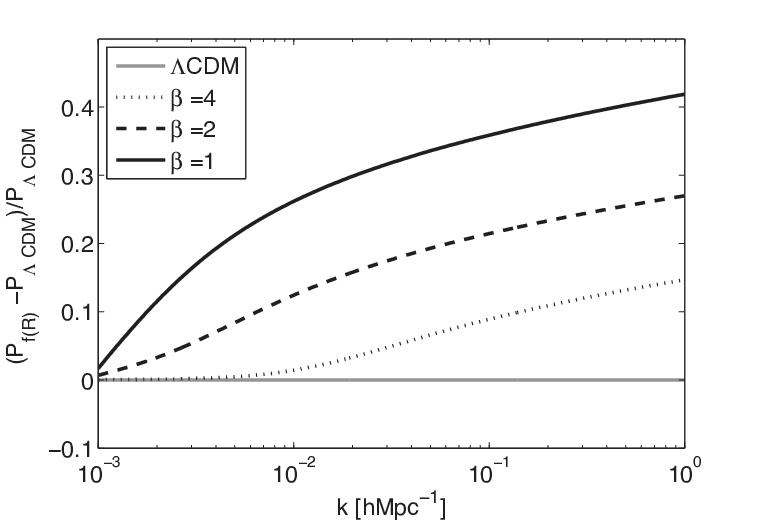
Instead of investigating the numerical result from MGCAMB directly, we can figure out the effect of $f(R)$ gravity on the matter power spectrum, $P(k)\sim\langle\delta_{m}^{2}\rangle$, based on the equation,

derived from Eqs. (9) - (14). If we set $f(R)=R-2\Lambda$ and $G_{eff}=G$, we recover the $\Lambda$CDM case. According to Eq. (23) and the definition of $G_{eff}$ in Eq. (17), the deviation of $\delta_{m}$ from the $\Lambda$CDM model can be estimated by the separation of variables,

where $\mu_{1}=f_{R}^{-1}$ and $\mu_{2}=\left(1+4k^{2}\,f_{RR}/a^{2}\,f_{R}\right)/\left(1+3k^{2}\,f_{RR}/a^{2}\,f_{R}\right)$. For the Starobinsky and exponential models, their first-order derivatives,

are both smaller than unity, so that $\mu_{1,2}$ are greater than unity. The first two viable conditions, $f_{R}>0$ and $f_{RR}>0$, guarantee that the numerator of $\mu_{2}$ is larger than its denominator. Furthermore, $\mu_{2}$ is enhanced by a large wavenumber $k$, corresponding to the matter power spectrum in the small scale. In all, the matter power spectra of the viable $f(R)$ gravity theories are always larger than that of the $\Lambda$CDM model as explicitly shown in Fig. 1, where the density of dark energy is fixed to be $\Omega_{DE}\sim 73\%$ and neutrino masses are taken to be zero.

The deviation between the Starobinsky (exponential) and $\Lambda$CDM models is proportional to $(R_{c}/R)^{2n}$ ($e^{-R/R_{c}}$). If the dark energy density $\rho_{\Lambda}$ is fixed at the present time ($z=0$), the characteristic curvature $R_{c}$ is inverse proportional to the model parameter, $R_{c}\sim 2\Lambda/\lambda(\beta)$, denoting that a smaller model parameter corresponds to a larger deviation for the matter power spectrum. As a result, we consider the model parameter space close to the lower bound of the viable condition ($\lambda,\beta\geq 1$ and $n\geq 2$) in the following calculations. In Fig. 2, we show the matter power spectra in the Starobinsky $(n=2)$ and exponential models, where the $\Lambda$CDM result is also given. As indicated above, a large enhancement of $f(R)$ gravity occurs at the large wavenumber $k$. There is an interesting phenomenon: the magnification of $P(k)$ in the Starobinsky model is more greater than that in the exponential one within the same allowed viable model parameter (e.g., $\lambda=\beta$ and $R_{c}^{\mathrm{star}}=R_{c}^{\mathrm{exp}}$). Since there is an exponential decay in the Type-II models, it converges toward the $\Lambda$CDM result much faster than that in the Type-I ones as the curvature increases. Accordingly, it is possible to exist a much larger enhancement the Type-I model than that in the Type-II one.

To study the effect of massive neutrinos on the matter power spectrum, we first use the relation between the contributions of massive neutrinos to the total energy density, $\Omega_{\nu}$, and the total mass, $\Sigma m_{\nu}$, in unit of eV, given by

where $h$ is the reduced Hubble constant. The upper value at $95\%$ C.L. for the total neutrino mass constrained by the Planck data in the $\Lambda$CDM model [5], $\Sigma m_{\nu}<0.23\ \mathrm{eV}$, leads to $\Omega_{\nu}\leq 5\times 10^{-3}$. Although it is a rather small ratio to the total energy density, its effect on the matter power spectrum is still detectable, as mentioned in Sec. 1. As demonstrated in Fig 3, we see that the free streaming massive neutrino suppresses the growth of $P(k)$ in the subhorizon scale [11]. This effect of massive neutrinos on the matter power spectrum is opposite to that of $f(R)$ models [12]. As a result, the Type-I $f(R)$ models would allow a higher scale for the total neutrino mass than Type-II.