跳到论文正文
W Papers独立论文阅读器 arXiv:1411.3810 论文正文 计算阅读时间 · 0%
引用这篇论文根据当前论文元数据生成,正式投稿前建议核对。


License: arXiv.org perpetual non-exclusive license
arXiv:1411.3810v1 [cs.IT] 14 Nov 2014

Fundamental Limits of Blind Deconvolution
Part I: Ambiguity Kernel

Sunav Choudhary    and Urbashi Mitra ††thanks: This work has been funded in part by the following grants and organizations:˜ONR˜N00014-09-1-0700, AFOSR˜FA9550-12-1-0215, NSF˜CNS-0832186, NSF˜CNS-1213128 and NSF˜CCF-1117896. Parts of this paper were presented at the IEEE International Symposium on Information Theory (ISIT), Honolulu, Hawai’i, June 29 - July 4, 2014˜[1] and at the IEEE Global Conference on Signal and Information Processing (GlobalSIP), Atlanta, Georgia, Dec. 3-5, 2014˜[2].††thanks: S.˜Choudhary and U.˜Mitra are with the Ming Hsieh Department of Electrical Engineering, Viterbi School of Engineering, University of Southern California, Los Angeles CA 90089, USA (email: sunavcho@usc.edu, ubli@usc.edu).
Abstract

Blind deconvolution is an ubiquitous non-linear inverse problem in applications like wireless communications and image processing. This problem is generally ill-posed, and there have been efforts to use sparse models for regularizing blind deconvolution to promote signal identifiability. Part I of this two-part paper characterizes the ambiguity space of blind deconvolution and shows unidentifiability of this inverse problem for almost every pair of unconstrained input signals. The approach involves lifting the deconvolution problem to a rank one matrix recovery problem and analyzing the rank two null space of the resultant linear operator. A measure theoretically tight (parametric and recursive) representation of the key rank two null space is stated and proved. This representation is a novel foundational result for signal and code design strategies promoting identifiability under convolutive observation models. Part II of this paper analyzes the identifiability of sparsity constrained blind deconvolution and establishes surprisingly strong negative results on scaling laws for the sparsity-ambiguity trade-off.

Index Terms: 
Identifiability, rank one matrix recovery, blind deconvolution, parametric representation, rank two null space

Section I Introduction

Blind deconvolution is a challenging inverse problem that is ubiquitous in applications of signal processing, control theory and wireless communications like blind image restoration [3, 4], blind system identification [5, 6] and, blind channel estimation and equalization [7, 8, 9, 10, 11]. In the absence of additional constraints, blind deconvolution is known to be ill-posed and each application mentioned above imposes some form of prior knowledge on the underlying signal structures to render the inverse problem better behaved. Sparsity based models have been used extensively in the past decade to capture hidden signal structures in many applications of interest. Prominent examples of the exploitation of sparsity include natural images admitting sparse wavelet domain representations [12, 13], ultra wide band communication channels exhibiting sparsity in Doppler-delay domain representations [14, 15], and user preferences and topic models displaying low-rank structures [16, 17] (sparsity in eigenvalue domain). While there have been a few attempts at exploiting sparsity priors for blind deconvolution and related problems [18, 19, 20, 21, 22, 23], there does not appear to be a general characterization of identifiability of such sparse models, except with very restrictive constraints. For example, [18] assumes a single random subspace signal model as opposed to the more commonly used union of subspaces signal model in compressed sensing [24]. In this two-part paper, we prove some surprising negative results for signal identifiability in the non-sparse and sparsity constrained blind deconvolution problems, even for the single subspace model. For a principled approach to studying these negative results, the first part of the paper develops a measure theoretically tight characterization of the ambiguity space of blind deconvolution. Because of the simplicity of the linear convolution map, its (non-linear) kernel can be partially parametrized to yield an analytically useful representation that is instrumental in the derivation of our results. To the best of our knowledge, this is a novel parameterization that has not appeared elsewhere in literature. The second part [25] of this paper shows that the unfavorable sparsity-ambiguity trade-off results on identifiability are a consequence of the kernel of the linear convolution map being of large dimension (of the order of the signal dimension).

Subsection I-A Numerical Examples and Intuition

We present some constructive numerical examples illustrating the nature and source of unidentifiability for blind linear deconvolution. The discrete-time blind linear deconvolution problem can be stated as the task of recovering (up to scalar multiplicative ambiguities) the unknown signal pair (𝒙∗,𝒚∗)∈ℝm×ℝn\left(\bm{x}_{\ast},\bm{y}_{\ast}\right)\in\mathbb{R}^{m}\times\mathbb{R}^{n} from the observation of their noise free linear convolution 𝒛∗=𝒙∗⋆𝒚∗∈ℝm+n−1\bm{z}_{\ast}=\bm{x}_{\ast}\star\bm{y}_{\ast}\in\mathbb{R}^{m+n-1}. It is intuitive to see that if there exists another pair (𝒙,𝒚)∈ℝm×ℝn\left(\bm{x},\bm{y}\right)\in\mathbb{R}^{m}\times\mathbb{R}^{n} such that 𝒙⋆𝒚=𝒙∗⋆𝒚∗\bm{x}\star\bm{y}=\bm{x}_{\ast}\star\bm{y}_{\ast} but 𝒙\bm{x} and 𝒙∗\bm{x}_{\ast} are not collinear then (𝒙∗,𝒚∗)\left(\bm{x}_{\ast},\bm{y}_{\ast}\right) is unidentifiable (information theoretically impossible to recover uniquely). Below, we illustrate what can go wrong with blind deconvolution for 𝒦=ℝ11×ℝ7\mathcal{K}=\mathbb{R}^{11}\times\mathbb{R}^{7} (beside scalar multiplicative ambiguities).

Consider the vectors 𝒙1,𝒙2∈ℝ11\bm{x}_{1},\bm{x}_{2}\in\mathbb{R}^{11} and 𝒚1,𝒚2∈ℝ7\bm{y}_{1},\bm{y}_{2}\in\mathbb{R}^{7} assigned as

𝒙1\displaystyle\bm{x}_{1} =(1,0,1,0,0,0,0,0,1,0,1)T,\displaystyle=\left(1,0,1,0,0,0,0,0,1,0,1\right)^{\mathrm{T}}, 𝒚1\displaystyle\quad\bm{y}_{1} =(1,0,0,0,1,0,0)T,\displaystyle=\left(1,0,0,0,1,0,0\right)^{\mathrm{T}}, (1a)
𝒙2\displaystyle\bm{x}_{2} =(1,0,0,0,0,0,0,0,1,0,0)T,\displaystyle=\left(1,0,0,0,0,0,0,0,1,0,0\right)^{\mathrm{T}}, 𝒚2\displaystyle\quad\bm{y}_{2} =(1,0,1,0,1,0,1)T.\displaystyle=\left(1,0,1,0,1,0,1\right)^{\mathrm{T}}. (1b)

Clearly, 𝒙1\bm{x}_{1} and 𝒙2\bm{x}_{2} are linearly independent and a simple calculation reveals that

𝒙1⋆𝒚1=𝒙2⋆𝒚2=(1,0,1,0,1,0,1,0,1,0,1,0,1,0,1,0,0)T\bm{x}_{1}\star\bm{y}_{1}=\bm{x}_{2}\star\bm{y}_{2}=\left(1,0,1,0,1,0,1,0,1,0,1,0,1,0,1,0,0\right)^{\mathrm{T}} (2)

implying unidentifiability of both (𝒙1,𝒚1)\left(\bm{x}_{1},\bm{y}_{1}\right) and (𝒙2,𝒚2)\left(\bm{x}_{2},\bm{y}_{2}\right) within 𝒦=ℝ11×ℝ7\mathcal{K}=\mathbb{R}^{11}\times\mathbb{R}^{7}. A more non-trivial numerical example can be constructed using the vectors 𝒙3\bm{x}_{3}, 𝒙4\bm{x}_{4}, 𝒚3\bm{y}_{3} and 𝒚4\bm{y}_{4} (which are functions of 𝒙1\bm{x}_{1}, 𝒙2\bm{x}_{2}, 𝒚1\bm{y}_{1} and 𝒚2\bm{y}_{2} above), defined as

𝒙3=𝒙1​cos⁡π3−𝒙2​sin⁡π3=(−0.366,0,0.5,0,0,0,0,0,−0.366,0,0.5)T,\displaystyle\begin{split}\bm{x}_{3}&=\bm{x}_{1}\cos\frac{\pi}{3}-\bm{x}_{2}\sin\frac{\pi}{3}\\ &=\left(-0.366,0,0.5,0,0,0,0,0,-0.366,0,0.5\right)^{\mathrm{T}},\end{split} (3a)
𝒚3=𝒚1​sin⁡π6−𝒚2​cos⁡π6=(−0.366,0,−0.866,0,−0.366,0,−0.866)T,\displaystyle\begin{split}\bm{y}_{3}&=\bm{y}_{1}\sin\frac{\pi}{6}-\bm{y}_{2}\cos\frac{\pi}{6}\\ &=\left(-0.366,0,-0.866,0,-0.366,0,-0.866\right)^{\mathrm{T}},\end{split} (3b)
𝒙4=𝒙1​cos⁡π6−𝒙2​sin⁡π6=(0.366,0,0.866,0,0,0,0,0,0.366,0,0.866)T,\displaystyle\begin{split}\bm{x}_{4}&=\bm{x}_{1}\cos\frac{\pi}{6}-\bm{x}_{2}\sin\frac{\pi}{6}\\ &=\left(0.366,0,0.866,0,0,0,0,0,0.366,0,0.866\right)^{\mathrm{T}},\end{split} (3c)
𝒚4=𝒚1​sin⁡π3−𝒚2​cos⁡π3=(0.366,0,−0.5,0,0.366,0,−0.5)T.\displaystyle\begin{split}\bm{y}_{4}&=\bm{y}_{1}\sin\frac{\pi}{3}-\bm{y}_{2}\cos\frac{\pi}{3}\\ &=\left(0.366,0,-0.5,0,0.366,0,-0.5\right)^{\mathrm{T}}.\end{split} (3d)

Clearly, 𝒙3\bm{x}_{3} and 𝒙4\bm{x}_{4} are linearly independent and we observe that

𝒙3⋆𝒚3=(0.134,0,0.134,0,−0.299,0,0.134,0,OPEN−0.299,0,0.134,0,−0.299,0,0.134,0,−0.433)T=𝒙4⋆𝒚4\begin{split}\bm{x}_{3}\star\bm{y}_{3}&=\left(0.134,0,0.134,0,-0.299,0,0.134,0,\right.\\ &\quad\left.-0.299,0,0.134,0,-0.299,0,0.134,0,-0.433\right)^{\mathrm{T}}\\ &=\bm{x}_{4}\star\bm{y}_{4}\end{split} (4)

implying unidentifiability of both pairs (𝒙3,𝒚3)\left(\bm{x}_{3},\bm{y}_{3}\right) and (𝒙4,𝒚4)\left(\bm{x}_{4},\bm{y}_{4}\right) within 𝒦=ℝ11×ℝ7\mathcal{K}=\mathbb{R}^{11}\times\mathbb{R}^{7}.

Fig. 1: An illustration of rotational ambiguity in blind linear deconvolution. Assuming 𝒙1⟂𝒙2\bm{x}_{1}\perp\bm{x}_{2} and 𝒚1⟂𝒚2\bm{y}_{1}\perp\bm{y}_{2} in the figure, 𝒙1⋆𝒚1=𝒙2⋆𝒚2\bm{x}_{1}\star\bm{y}_{1}=\bm{x}_{2}\star\bm{y}_{2} implies 𝒙1′⋆𝒚1′=𝒙2′⋆𝒚2′\bm{x}_{1}^{\prime}\star\bm{y}_{1}^{\prime}=\bm{x}_{2}^{\prime}\star\bm{y}_{2}^{\prime} for any θ≠ϕ\theta\neq\phi.

The construction used in (3) illustrates a form of rotational ambiguity that generalizes to produce a family of unidentifiable pairs in 𝒦\mathcal{K}. Fig. 1 represents a pictorial depiction of the following construction. Let 𝒛0=𝒙1⋆𝒚1=𝒙2⋆𝒚2\bm{z}_{0}=\bm{x}_{1}\star\bm{y}_{1}=\bm{x}_{2}\star\bm{y}_{2} denote the common convolved output in (2). Consider the parameterized vectors 𝒙1′,𝒙2′∈ℝ11\bm{x}_{1}^{\prime},\bm{x}_{2}^{\prime}\in\mathbb{R}^{11} and 𝒚1′,𝒚2′∈ℝ7\bm{y}_{1}^{\prime},\bm{y}_{2}^{\prime}\in\mathbb{R}^{7} defined by

𝒙1′\displaystyle\bm{x}_{1}^{\prime} =𝒙1​cos⁡θ−𝒙2​sin⁡θ,\displaystyle=\bm{x}_{1}\cos\theta-\bm{x}_{2}\sin\theta, 𝒚1′\displaystyle\quad\bm{y}_{1}^{\prime} =𝒚1​sin⁡ϕ−𝒚2​cos⁡ϕ,\displaystyle=\bm{y}_{1}\sin\phi-\bm{y}_{2}\cos\phi, (5a)
𝒙2′\displaystyle\bm{x}_{2}^{\prime} =𝒙1​cos⁡ϕ−𝒙2​sin⁡ϕ,\displaystyle=\bm{x}_{1}\cos\phi-\bm{x}_{2}\sin\phi, 𝒚2′\displaystyle\quad\bm{y}_{2}^{\prime} =𝒚1​sin⁡θ−𝒚2​cos⁡θ,\displaystyle=\bm{y}_{1}\sin\theta-\bm{y}_{2}\cos\theta, (5b)

where θ≠ϕ\theta\neq\phi are the parameters, and {𝒙1,𝒙2,𝒚1,𝒚2}\left\{\bm{x}_{1},\bm{x}_{2},\bm{y}_{1},\bm{y}_{2}\right\} acts as the set of seed vectors driving the above transformation. Clearly, linear independence of 𝒙1\bm{x}_{1} and 𝒙2\bm{x}_{2} and θ≠ϕ\theta\neq\phi imply that 𝒙1′\bm{x}_{1}^{\prime} and 𝒙2′\bm{x}_{2}^{\prime} are linearly independent. Simple algebraic manipulations reveal that

𝒙1′⋆𝒚1′=𝒙1⋆𝒚1​cos⁡θ​sin⁡ϕ+𝒙2⋆𝒚2​sin⁡θ​cos⁡ϕ−𝒙2⋆𝒚1sinθsinϕ−𝒙1⋆𝒚2cosθcosϕ=𝒛0​sin⁡(θ+ϕ)−𝒙2⋆𝒚1sinθsinϕ−𝒙1⋆𝒚2cosθcosϕ\displaystyle\begin{split}\bm{x}_{1}^{\prime}\star\bm{y}_{1}^{\prime}&=\bm{x}_{1}\star\bm{y}_{1}\cos\theta\sin\phi+\bm{x}_{2}\star\bm{y}_{2}\sin\theta\cos\phi\\ &\quad-\bm{x}_{2}\star\bm{y}_{1}\sin\theta\sin\phi-\bm{x}_{1}\star\bm{y}_{2}\cos\theta\cos\phi\\ &=\bm{z}_{0}\sin\left(\theta+\phi\right)\\ &\quad-\bm{x}_{2}\star\bm{y}_{1}\sin\theta\sin\phi-\bm{x}_{1}\star\bm{y}_{2}\cos\theta\cos\phi\end{split} (6a)
and,
𝒙2′⋆𝒚2′=𝒙1⋆𝒚1​cos⁡ϕ​sin⁡θ+𝒙2⋆𝒚2​sin⁡ϕ​cos⁡θ−𝒙2⋆𝒚1sinϕsinθ−𝒙1⋆𝒚2cosϕcosθ=𝒛0​sin⁡(θ+ϕ)−𝒙2⋆𝒚1sinθsinϕ−𝒙1⋆𝒚2cosθcosϕ.\displaystyle\begin{split}\bm{x}_{2}^{\prime}\star\bm{y}_{2}^{\prime}&=\bm{x}_{1}\star\bm{y}_{1}\cos\phi\sin\theta+\bm{x}_{2}\star\bm{y}_{2}\sin\phi\cos\theta\\ &\quad-\bm{x}_{2}\star\bm{y}_{1}\sin\phi\sin\theta-\bm{x}_{1}\star\bm{y}_{2}\cos\phi\cos\theta\\ &=\bm{z}_{0}\sin\left(\theta+\phi\right)\\ &\quad-\bm{x}_{2}\star\bm{y}_{1}\sin\theta\sin\phi-\bm{x}_{1}\star\bm{y}_{2}\cos\theta\cos\phi.\end{split} (6b)

Since (6a) and (6b) have the same r.h.s., both (𝒙1′,𝒚1′)\left(\bm{x}_{1}^{\prime},\bm{y}_{1}^{\prime}\right) and (𝒙2′,𝒚2′)\left(\bm{x}_{2}^{\prime},\bm{y}_{2}^{\prime}\right) are unidentifiable within 𝒦=ℝ11×ℝ7\mathcal{K}=\mathbb{R}^{11}\times\mathbb{R}^{7}. Since (θ,ϕ)∈[0,π)2\left(\theta,\phi\right)\in[0,\pi)^{2} describes a two dimensional parameter space, (6) implies that the unidentifiable subset of 𝒦\mathcal{K} is at least two dimensional. Notice that the aforementioned construction for unidentifiable signal pairs (i.e. the rotational ambiguity) remains true, even if the domain of the vectors 𝒙1′\bm{x}_{1}^{\prime} and 𝒙2′\bm{x}_{2}^{\prime} is restricted to an annulus 𝒙1′,𝒙2′∈{𝒘∈ℝ11|γ≤‖𝒘‖2≤δ}\bm{x}_{1}^{\prime},\bm{x}_{2}^{\prime}\in\left\{\bm{w}\in\mathbb{R}^{11}\mathrel{}\middle|\mathrel{}\gamma\leq\left\lVert\bm{w}\right\rVert_{2}\leq\delta\right\} for some γ≠δ\gamma\neq\delta.

Subsection I-B Related Work

Prior research on blind system and channel identification [5, 7, 11] has mainly focused on single-in-multiple-out (SIMO) and multiple-in-multiple-out (MIMO) systems, also known as the blind multi-channel finite-impulse-response (FIR) estimation problem. These systems have multiple output channels that need to be estimated from the observed outputs when the channels are driven by either a single source (SIMO system) or multiple sources (MIMO system). A key property necessary for successful identifiability and recovery of the multiple channel vectors is that the channels should display sufficient diversity or richness either stochastically (cyclostationary second order statistics) [26, 27, 7] or deterministically (no common zero across all channels) [28, 29, 11, 30, 31]. As pointed out in [26, 10], such diversity is generally unavailable in the single-in-single-out (SISO) systems thus making them extremely challenging. However, SISO systems are our primary concern due to their equivalence to blind deconvolution problems. In this paper, we shall not be concerned with stochastic formulations where multiple realizations of the channel are observed to infer empirical statistics. Instead, we shall consider non-sparse (here, in Part I) and sparse (in Part II) channel instances and characterize their instance identifiabilities. When blind deconvolution is treated as a channel estimation problem, [32] shows that guard intervals of sufficient length between blocks of transmitted symbols enable successful blind channel identification, even for the deterministic SISO system type. More specifically, for an nn length channel impulse response (CIR) a guard interval of length n−1n-1 is needed between consecutive blocks of transmitted source symbols, resulting in an absence of any inter-block or inter-symbol interference (ISI) in the convolved output of the channel. We consider scenarios involving ISI and show unidentifiability w.r.t. a wide variety of domain restrictions. Although our definition of identifiability is similar to that in [32], our results are substantially different in nature. Firstly, we deal with real fields (not algebraically closed) and with sparse subsets of real vector spaces (induced by measures that are not absolutely continuous w.r.t. the Lebesgue measure) as opposed to the algebraically closed complex fields and vector spaces considered in [32]. This requires different proof techniques. Secondly, we focus on unidentifiability results and characterize the dimension of the unidentifiable subsets in addition to showing existence results. Furthermore, our proofs constructively show unidentifiable subsets as opposed to non-constructive existence proofs.

To the best of our knowledge, blind deconvolution was cast as a rank one matrix recovery problem first in [33]; we adopted this framework in our earlier works [34, 35, 36] on characterization of identifiability in general bilinear inverse problems. Herein, we specifically consider the blind deconvolution problem and characterize its inherent unidentifiability under some application-motivated sparsity and subspace constraints. Further, [33] focused on developing heuristic algorithms for the deconvolution problem and did not explicitly address identifiability. The subsequent paper [18], by the authors of [33], does (implicitly) address identifiability (through a study of recoverability by convex programming) but assumes the knowledge of the support of the sparse signal. Although blind deconvolution is an instance of a bilinear inverse problem, the present work differs significantly from our earlier work [36] in two ways. Firstly, [36] focused on identifiability results (analogous to achievability results in information theory) whereas the present paper derives unidentifiability results (akin to converse/impossibility results in information theory). Secondly, Part II of this paper [25] explores more explicit sparsity priors motivated by applications like cooperative communication [37, 38], channel estimation for wide-band communication [15] and musical source separation [21], whereas [36] developed the theory of regularized bilinear inverse problems more abstractly, making assumptions no more specific than non-convex cone constrained priors. A consequence of focusing specifically on blind deconvolution is that we are able to develop tight converse bounds that match our achievability bounds in [36]. The tractability of this analysis hinges on the structural simplicity of the convolution operator after lifting.

To rigorously justify the dimension related results in both parts of the paper, we call upon the theoretical framework of the Hausdorff dimension of sets in metric spaces. A moderately detailed introduction to the topic can be found in [39]. For the sake of readability, we provide a short review of the concept and some of the useful properties in Part II, Section II-C of the paper.

Subsection I-C Contributions and Organization

In this work, we quantify unidentifiability for certain families of noiseless sparse and non-sparse blind deconvolution problems under a non-asymptotic and non-statistical setup. Specifically, given model orders m,n∈ℤ+m,n\in\mathbb{Z}^{+}, Part I of the paper develops a parameterization of the ambiguity kernel for blind linear deconvolution and shows that almost every input (𝒙∗,𝒚∗)⊆ℝm×ℝn\left(\bm{x}_{\ast},\bm{y}_{\ast}\right)\subseteq\mathbb{R}^{m}\times\mathbb{R}^{n} is unidentifiable under blind deconvolution in the absence of further constraints. Furthermore, the characterization developed herein is used in Part II of the paper to investigate some application driven choices of the separable domain restriction (𝒙∗,𝒚∗)∈𝒦⊆ℝm×ℝn\left(\bm{x}_{\ast},\bm{y}_{\ast}\right)\in\mathcal{K}\subseteq\mathbb{R}^{m}\times\mathbb{R}^{n} and establish that these restrictions are insufficient to guarantee identifiability of the vectors 𝒙∗\bm{x}_{\ast} and 𝒚∗\bm{y}_{\ast} from their linearly convolved resultant vector 𝒛∗=𝒙∗⋆𝒚∗\bm{z}_{\ast}=\bm{x}_{\ast}\star\bm{y}_{\ast}. Our approach leads to the following novelties for Part I (refer to [25] for contributions of Part II of the paper).

  1. 1.

    We are able to analyze unidentifiability in blind deconvolution by studying the rank constrained null space of a linear operator on matrices. We explicitly demonstrate the almost everywhere unidentifiable nature of unconstrained blind deconvolution by constructing families of adversarial signal pairs for even model orders mm and nn. This is a much stronger unidentifiability result than any counterparts in the literature.

  2. 2.

    We state and prove a measure theoretically tight, non-linear, partially parametric and partially recursive characterization of the rank two null space of the lifted linear convolution map. To the best of our knowledge, this is a new result. Characterizing the rank two null space is useful for a variety of applications, including the study of scaling laws in bilinear inverse problems [36]. Our proofs are constructive and demonstrate a rotational ambiguity phenomenon in general bilinear inverse problems which is the cause of existence of a large dimensional set of unidentifiable input pairs in blind deconvolution.

The rest of the paper is organized as follows. Section II describes the system model, sets up the notion of identifiability up to a suitably defined equivalence class, and presents the lifted reformulation of the blind deconvolution problem as a rank one matrix recovery problem. Section III develops a novel, measure theoretically tight characterization of the rank two null space of the lifted linear convolution map, exploiting both parametric as well as recursive definitions. Section IV presents the key unidentifiability result for non-sparse blind deconvolution, exploiting the parametric representation of the rank two null space of the lifted linear convolution map developed in Section III. Section V concludes the paper. Detailed proofs of all the results in the paper appear in the Appendices A-E.

Subsection I-D Notational Conventions

All vectors are assumed to be column vectors unless stated otherwise. We shall use lowercase boldface alphabets to denote column vectors (e.g. 𝒂\bm{a}) and uppercase boldface alphabets to denote matrices (e.g. 𝑨\bm{A}). The MATLAB® indexing rules will be used to denote parts of a vector/matrix (e.g. 𝑨(2:3,4:6)\bm{A}\left(2:3,4:6\right) denotes the sub-matrix of 𝑨\bm{A} formed by the rows {2,3}\left\{2,3\right\} and columns {4,5,6}\left\{4,5,6\right\}). The all zero vector/matrix shall be denoted by 𝟎\bm{0} and its dimension would be clear from the usage context. For matrices, (⋅)T\left(\cdot\right)^{\mathrm{T}} and rank(⋅)\mathop{\mathrm{rank}}\left(\cdot\right) respectively return the transpose and rank of their argument. Special sets are denoted by uppercase blackboard bold font (e.g. ℝ\mathbb{R} for real numbers). Other sets are denoted by uppercase calligraphic font (e.g. 𝒮\mathcal{S}). Linear operators on matrices are denoted by uppercase script font (e.g. 𝒮\mathscr{S}). For any matrix 𝑴\bm{M}, we denote its column space by 𝒞⁡(𝑴)\mathcal{C}\left(\bm{M}\right). The standard Euclidean inner product on a vector space will be denoted by ⟨⋅,⋅⟩\left\langle\cdot,\cdot\right\rangle and the underlying vector space will be clear from the usage context.

When we refer to the ‘dimension’ of a set, we shall mean the Hausdorff dimension of the set. To avoid unnecessarily heavy notation, we shall adopt the following convention: The use of both vector variables (like 𝒙\bm{x}, 𝒚\bm{y}, 𝒖\bm{u}, 𝒗\bm{v}, etc.) as well as matrix variables (like 𝑿\bm{X}, 𝒀\bm{Y}, etc.) is allowed to differ across theorems and proofs (and even across different subparts of the same proof) with the understanding that their meanings are restricted to the scope of the individual theorems (and proofs). This facilitates the reuse of the same variable names across different theorems with distinct meanings without confusion.

Section II System Model

Subsection II-A The Blind Deconvolution Problem

We shall consider the noiseless linear convolution system model

𝒛=𝒙⋆𝒚,\bm{z}=\bm{x}\star\bm{y}, (7)

where (𝒙,𝒚)\left(\bm{x},\bm{y}\right) denotes the pair of unknown signals with a given domain restriction (𝒙,𝒚)∈𝒦⊆ℝm×ℝn\left(\bm{x},\bm{y}\right)\in\mathcal{K}\subseteq\mathbb{R}^{m}\times\mathbb{R}^{n}, ⋆:ℝm×ℝn→ℝm+n−1\star\colon\mathbb{R}^{m}\times\mathbb{R}^{n}\to\mathbb{R}^{m+n-1} denotes the linear convolution map, and 𝒛∈ℝm+n−1\bm{z}\in\mathbb{R}^{m+n-1} is the vector of observations given by

𝒛⁡(l)={∑j=1min⁡(l,m)𝒙⁡(j)​𝒚​(l+1−j),1≤l≤n,∑j=l+1−nmin⁡(l,m)𝒙⁡(j)​𝒚​(l+1−j),1≤l−n≤m−1.\bm{z}\left(l\right)=\begin{cases}{\displaystyle\sum_{j=1}^{\min\left(l,m\right)}\bm{x}\left(j\right)\bm{y}\left(l+1-j\right)},&1\leq l\leq n,\\ {\displaystyle\sum_{j=l+1-n}^{\min\left(l,m\right)}\bm{x}\left(j\right)\bm{y}\left(l+1-j\right)},&1\leq l-n\leq m-1.\end{cases} (8)

We are interested in solving for the vectors 𝒙\bm{x} and 𝒚\bm{y} from the noiseless observation 𝒛\bm{z} in (7). The blind linear deconvolution problem corresponding to (7) is represented by the feasibility problem

find\displaystyle\text{find} (𝒙,𝒚)\displaystyle\left(\bm{x},\bm{y}\right) (P1)
subject to\displaystyle\text{subject to} 𝒙⋆𝒚=𝒛,\displaystyle\bm{x}\star\bm{y}=\bm{z},
(𝒙,𝒚)∈𝒦.\displaystyle\left(\bm{x},\bm{y}\right)\in\mathcal{K}.

We are interested in whether the pair (𝒙,𝒚)\left(\bm{x},\bm{y}\right) can be uniquely identified in a meaningful sense. We assume that the lengths (or model orders) mm and nn, respectively, of vectors 𝒙\bm{x} and 𝒚\bm{y} are fixed and known a priori. Notice that the deconvolution problem (P1) has an inherent scaling ambiguity due to the identity

𝒙⋆𝒚=α​𝒙⋆1α​𝒚,∀α≠0,\bm{x}\star\bm{y}=\alpha\bm{x}\star\frac{1}{\alpha}\bm{y},\quad\forall\alpha\neq 0, (9)

stemming from the bi-linearity of the convolution operator. Thus, any meaningful definition of identifiability for blind deconvolution must disregard this type of scaling ambiguity. This leads us to the following definition of identifiability.

Definition 1 (Identifiability).

A vector pair (𝐱,𝐲)∈𝒦⊆ℝm×ℝn\left(\bm{x},\bm{y}\right)\in\mathcal{K}\subseteq\mathbb{R}^{m}\times\mathbb{R}^{n} is identifiable with respect to the linear convolution map ⋆\star, if ∀(𝐱′,𝐲′)∈𝒦⊆ℝm×ℝn\forall\left(\bm{x}^{\prime},\bm{y}^{\prime}\right)\in\mathcal{K}\subseteq\mathbb{R}^{m}\times\mathbb{R}^{n} satisfying 𝐱⋆𝐲=𝐱′⋆𝐲′\bm{x}\star\bm{y}=\bm{x}^{\prime}\star\bm{y}^{\prime}, ∃α≠0\exists\alpha\neq 0 such that (𝐱′,𝐲′)=(α​𝐱,1α​𝐲)\left(\bm{x}^{\prime},\bm{y}^{\prime}\right)=\left(\alpha\bm{x},\frac{1}{\alpha}\bm{y}\right).

This definition is in the same spirit as the notion of noise free identifiability described in [32], but restricted to a set 𝒦⊆ℝm×ℝn\mathcal{K}\subseteq\mathbb{R}^{m}\times\mathbb{R}^{n}. It is easy to see that Definition 1 induces an equivalence structure on the set of identifiable pairs in 𝒦\mathcal{K}, and identifiability refers to the identification of the equivalence class in 𝒦\mathcal{K} that generated the observation 𝒛\bm{z} in (7).

Subsection II-B Lifting

While Problem (P1) is an accurate representation of a blind deconvolution problem, it is not easily amenable to an identifiability analysis in the sense of Definition 1. We use the lifting technique from optimization [40] to rewrite Problem (P1) as a rank minimization problem subject to linear equality constraints [34, 33]; a form that is better suited for an identifiability analysis,

minimize𝑾\displaystyle\underset{\bm{W}}{\text{minimize}} rank(𝑾)\displaystyle\mathop{\mathrm{rank}}\left(\bm{W}\right) (P2)
subject to\displaystyle\text{subject to} 𝒮⁡(𝑾)=𝒛,\displaystyle\mathscr{S}\left(\bm{W}\right)=\bm{z},
𝑾∈𝒲,\displaystyle\bm{W}\in\mathcal{W},

where 𝒲⊆ℝm×n\mathcal{W}\subseteq\mathbb{R}^{m\times n} is any set satisfying

𝒲​⋂{𝑾∈ℝm×n|rank(𝑾)≤1}={𝒙​𝒚T|(𝒙,𝒚)∈𝒦},\mathcal{W}\bigcap\left\{\bm{W}\in\mathbb{R}^{m\times n}\mathrel{}\middle|\mathrel{}\mathop{\mathrm{rank}}\left(\bm{W}\right)\leq 1\right\}=\left\{\bm{x}\bm{y}^{\mathrm{T}}\mathrel{}\middle|\mathrel{}\left(\bm{x},\bm{y}\right)\in\mathcal{K}\right\}, (10)

and 𝒮:ℝm×n→ℝm+n−1\mathscr{S}\colon\mathbb{R}^{m\times n}\to\mathbb{R}^{m+n-1} is a linear operator which can be deterministically constructed from the linear convolution map. We shall refer to 𝒮\mathscr{S} as the lifted linear convolution map. Specifically, 𝒮⁡(⋅)\mathscr{S}\left(\cdot\right) is the unique linear operator that satisfies

𝒮⁡(𝒙​𝒚T)=𝒙⋆𝒚,∀(𝒙,𝒚)∈ℝm×ℝn.\mathscr{S}\left(\bm{x}\bm{y}^{\mathrm{T}}\right)=\bm{x}\star\bm{y},\quad\forall\left(\bm{x},\bm{y}\right)\in\mathbb{R}^{m}\times\mathbb{R}^{n}. (11)

By construction, the optimal solution to Problem (P2) is a rank one matrix 𝑾opt\bm{W}_{\text{opt}} and its singular value decomposition 𝑾opt=σopt​𝒖opt​𝒗optT\bm{W}_{\text{opt}}=\sigma_{\text{opt}}\bm{u}_{\text{opt}}\bm{v}_{\text{opt}}^{\mathrm{T}} yields a solution (𝒙,𝒚)opt=(σopt​𝒖opt,σopt​𝒗opt)\left(\bm{x},\bm{y}\right)_{\text{opt}}=\left(\sqrt{\sigma_{\text{opt}}}\bm{u}_{\text{opt}},\sqrt{\sigma_{\text{opt}}}\bm{v}_{\text{opt}}\right) to Problem (P1). The exact steps involved in the lifting technique and a proof of equivalence between the lifted and the original problems, in the much broader context of bilinear inverse problems, are available in [36]. Our unidentifiability results in Section IV will be based on an analysis of Problem (P2).

Remark 1.

It is well known from functional analysis [41] that any finite dimensional linear operation can be decomposed into a set of inner product operations that collectively define the linear operation. The lifted linear convolution map 𝒮⁡(⋅)\mathscr{S}\left(\cdot\right) can be decomposed into a functionally equivalent set, comprising of (m+n−1)\left(m+n-1\right) matrices, using coordinate projections. Let 𝐒j∈ℝm×n\bm{S}_{j}\in\mathbb{R}^{m\times n} denote the jthj^{\text{th}} matrix in the decomposition and ϕj:ℝm+n−1→ℝ\phi_{j}\colon\mathbb{R}^{m+n-1}\to\mathbb{R} denote the jthj^{\text{th}} coordinate projection operator of (m+n−1)\left(m+n-1\right) dimensional vectors to scalars, i.e. if 𝐳∈ℝm+n−1\bm{z}\in\mathbb{R}^{m+n-1} then ϕj​(𝐳)=𝐳​(j)\phi_{j}\left(\bm{z}\right)=\bm{z}\left(j\right), for 1≤j≤m+n−11\leq j\leq m+n-1. For all (𝐱,𝐲)∈ℝm×ℝn\left(\bm{x},\bm{y}\right)\in\mathbb{R}^{m}\times\mathbb{R}^{n}, we have the relation

ϕj​(𝒙⋆𝒚)=ϕj∘𝒮⁡(𝒙​𝒚T)=⟨𝑺j,𝒙​𝒚T⟩=𝒙T𝑺j𝒚,∀1≤j≤m+n−1,\begin{split}\phi_{j}\left(\bm{x}\star\bm{y}\right)&=\phi_{j}\circ\mathscr{S}\left(\bm{x}\bm{y}^{\mathrm{T}}\right)=\left\langle\bm{S}_{j},\bm{x}\bm{y}^{\mathrm{T}}\right\rangle\\ &=\bm{x}^{\mathrm{T}}\bm{S}_{j}\bm{y},\quad\forall 1\leq j\leq m+n-1,\end{split} (12)

where ⟨⋅,⋅⟩\left\langle\cdot,\cdot\right\rangle denotes the trace inner product in the space of matrices ℝm×n\mathbb{R}^{m\times n}. By way of exposition, we compute 𝐒3\bm{S}_{3} for (m,n)=(3,4)\left(m,n\right)=\left(3,4\right). Let (𝐱,𝐲)∈ℝ3×ℝ4\left(\bm{x},\bm{y}\right)\in\mathbb{R}^{3}\times\mathbb{R}^{4}. Invoking the expansion in (8), we have

ϕ3​(𝒙⋆𝒚)=∑j=13𝒙⁡(j)​𝒚​(4−j)=[𝒙⁡(1),𝒙⁡(2),𝒙⁡(3)]​[001001001000]​[𝒚⁡(1)𝒚⁡(2)𝒚⁡(3)𝒚⁡(4)]=𝒙T​𝑺3​𝒚.\begin{split}\phi_{3}\left(\bm{x}\star\bm{y}\right)&=\sum_{j=1}^{3}\bm{x}\left(j\right)\bm{y}\left(4-j\right)\\ &=\left[\bm{x}\left(1\right),\bm{x}\left(2\right),\bm{x}\left(3\right)\right]\begin{bmatrix}0&0&1&0\\ 0&1&0&0\\ 1&0&0&0\end{bmatrix}\begin{bmatrix}\bm{y}\left(1\right)\\ \bm{y}\left(2\right)\\ \bm{y}\left(3\right)\\ \bm{y}\left(4\right)\end{bmatrix}\\ &=\bm{x}^{\mathrm{T}}\bm{S}_{3}\bm{y}.\end{split} (13)

The matrix 𝐒3∈ℝ3×4\bm{S}_{3}\in\mathbb{R}^{3\times 4} is given by

𝑺3​(k,l)={1,k+l=4,0,otherwise,\bm{S}_{3}\left(k,l\right)=\begin{cases}1,&k+l=4,\\ 0,&\text{otherwise,}\end{cases} (14)

for 1≤k≤31\leq k\leq 3 and 1≤l≤41\leq l\leq 4. In general, it is not hard to see that the matrices 𝐒j\bm{S}_{j}, 1≤j≤m+n−11\leq j\leq m+n-1, are Hankel matrices in {0,1}m×n⊂ℝm×n\left\{0,1\right\}^{m\times n}\subset\mathbb{R}^{m\times n} specified as

𝑺j​(k,l)={1,k+l=j+1,0,otherwise,\bm{S}_{j}\left(k,l\right)=\begin{cases}1,&k+l=j+1,\\ 0,&\text{otherwise,}\end{cases} (15)

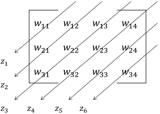
for 1≤k≤m1\leq k\leq m, and 1≤l≤n1\leq l\leq n. Fig. 2 illustrates these matrices forming the decomposition corresponding to the lifted linear convolution operator 𝒮⁡(⋅)\mathscr{S}\left(\cdot\right) for the case of (m,n)=(3,4)\left(m,n\right)=\left(3,4\right).

Refer to caption
Fig. 2: Lifted matrices 𝑺k∈ℝm×n\bm{S}_{k}\in\mathbb{R}^{m\times n} for linear convolution map with m=3m=3, n=4n=4 and 1≤k≤m+n−11\leq k\leq m+n-1.

Subsection II-C Anti-Diagonal Sum Interpretation

We illustrate an interpretation of the lifted linear convolution operator that forms a key step in the proofs of our results in Section III. Let 𝒛∈ℝm+n−1\bm{z}\in\mathbb{R}^{m+n-1} be the result of applying the lifted convolution map 𝒮⁡(⋅)\mathscr{S}\left(\cdot\right) to the matrix 𝑾∈ℝm×n\bm{W}\in\mathbb{R}^{m\times n}, i.e. 𝒮⁡(𝑾)=𝒛\mathscr{S}\left(\bm{W}\right)=\bm{z} and consider the case (m,n)=(3,4)\left(m,n\right)=\left(3,4\right) in Fig. 3 as an example. It is clear that 𝒛⁡(j)\bm{z}\left(j\right) is formed by adding all elements of 𝑾\bm{W} that lie on the jthj^{\text{th}} arrow (the jthj^{\text{th}} anti-diagonal) in Fig. 3. In other words, the linear operator 𝒮⁡(⋅)\mathscr{S}\left(\cdot\right) sums elements of its argument along the anti-diagonals to generate the output. From the definition of linear convolution in (8), it is easy to see that this interpretation of the lifted convolution operator holds regardless of the numerical values of the dimensions mm and nn.

Refer to caption
Fig. 3: Illustration of the anti-diagonal sum interpretation of the lifted linear convolution operator 𝒮⁡(⋅)\mathscr{S}\left(\cdot\right) for (m,n)=(3,4)\left(m,n\right)=\left(3,4\right) satisfying 𝒮⁡(𝑾)=𝒛\mathscr{S}\left(\bm{W}\right)=\bm{z}. The shorthand wk​l=𝑾⁡(k,l)w_{kl}=\bm{W}\left(k,l\right) has been used with 1≤k≤m=31\leq k\leq m=3 and 1≤l≤n=41\leq l\leq n=4.

As an immediate consequence, we make the following observation (also an important part of the proofs to the results in Section III). Let 𝑾′∈ℝ(m−1)×(n−1)\bm{W}^{\prime}\in\mathbb{R}^{\left(m-1\right)\times\left(n-1\right)} be any arbitrary matrix and we consider the matrices 𝑾1,𝑾2∈ℝm×n\bm{W}_{1},\bm{W}_{2}\in\mathbb{R}^{m\times n} constructed as

𝑾1=[𝟎𝑾′0𝟎T],𝑾2=[𝟎T0𝑾′𝟎].\bm{W}_{1}=\begin{bmatrix}\bm{0}&\bm{W}^{\prime}\\ 0&\bm{0}^{\mathrm{T}}\end{bmatrix},\quad\bm{W}_{2}=\begin{bmatrix}\bm{0}^{\mathrm{T}}&0\\ \bm{W}^{\prime}&\bm{0}\end{bmatrix}. (16)

Clearly, the elements of 𝑾2\bm{W}_{2} along the jthj^{\text{th}} anti-diagonal are a circularly shifted copy of the elements of 𝑾1\bm{W}_{1} along the jthj^{\text{th}} anti-diagonal, i.e. 𝑾2\bm{W}_{2} is formed by shifting down the elements of 𝑾1\bm{W}_{1} by one unit along the anti-diagonals. In particular, this implies that the sum of elements along the jthj^{\text{th}} anti-diagonal is the same for both 𝑾1\bm{W}_{1} and 𝑾2\bm{W}_{2}. Using the sum along anti-diagonals interpretation of the lifted linear convolution map 𝒮⁡(⋅)\mathscr{S}\left(\cdot\right), we have

𝒮⁡(𝑾1)=𝒮⁡(𝑾2)=[0𝒮′​(𝑾′)0],\mathscr{S}\left(\bm{W}_{1}\right)=\mathscr{S}\left(\bm{W}_{2}\right)=\begin{bmatrix}0\\ \mathscr{S}^{\prime}\left(\bm{W}^{\prime}\right)\\ 0\end{bmatrix}, (17)

where 𝒮′:ℝ(m−1)×(n−1)→ℝm+n−3\mathscr{S}^{\prime}\mathpunct{:}\mathbb{R}^{(m-1)\times(n-1)}\to\mathbb{R}^{m+n-3} denotes the lifted linear convolution map in one lower dimension than 𝒮⁡(⋅)\mathscr{S}\left(\cdot\right) w.r.t. both rows and columns. Thus, 𝑾1\bm{W}_{1} and 𝑾2\bm{W}_{2} are indistinguishable under the action of the linear operator 𝒮⁡(⋅)\mathscr{S}\left(\cdot\right).

Section III Parameterizing the Rank Two Null Space

Suppose that 𝒮⁡(⋅)\mathscr{S}\left(\cdot\right) is the lifted linear operator corresponding to the linear convolution map. We denote the rank two null space of 𝒮⁡(⋅)\mathscr{S}\left(\cdot\right) by 𝒩⁡(𝒮,2)\mathcal{N}\left(\mathscr{S},2\right) which is defined as [36]

𝒩(𝒮,2)≜{𝑸∈ℝm×n|rank(𝑸)≤2,𝒮(𝑸)=𝟎}.\mathcal{N}\left(\mathscr{S},2\right)\triangleq\left\{\bm{Q}\in\mathbb{R}^{m\times n}\mathrel{}\middle|\mathrel{}\mathop{\mathrm{rank}}\left(\bm{Q}\right)\leq 2,\,\mathscr{S}\left(\bm{Q}\right)=\bm{0}\right\}. (18)

In this section, we establish a partially parametric and partially dimension recursive characterization of 𝒩⁡(𝒮,2)\mathcal{N}\left(\mathscr{S},2\right) that is critical to our subsequent results in Section IV. We first establish Lemma 1 that describes a subset of 𝒩⁡(𝒮,2)\mathcal{N}\left(\mathscr{S},2\right). Proposition 1 shows existence of subsets of 𝒩⁡(𝒮,2)\mathcal{N}\left(\mathscr{S},2\right) not covered by Lemma 1. Theorem 1 then provides an almost everywhere characterization of 𝒩⁡(𝒮,2)\mathcal{N}\left(\mathscr{S},2\right). Finally, Proposition 2 shows existence of subsets of 𝒩⁡(𝒮,2)\mathcal{N}\left(\mathscr{S},2\right) that are not covered by Theorem 1. We shall make use of the fact that the rank one null space of the linear convolution operator is trivial, i.e.

𝒩(𝒮,1)≜{𝑸∈ℝm×n|rank(𝑸)≤1,𝒮(𝑸)=𝟎}={𝟎},\mathcal{N}\left(\mathscr{S},1\right)\triangleq\left\{\bm{Q}\in\mathbb{R}^{m\times n}\mathrel{}\middle|\mathrel{}\mathop{\mathrm{rank}}\left(\bm{Q}\right)\leq 1,\,\mathscr{S}\left(\bm{Q}\right)=\bm{0}\right\}=\left\{\bm{0}\right\}, (19)

which follows from interpreting convolution as polynomial multiplication, since the product of two real polynomials is identically zero if and only if at least one of them is identically zero.

Lemma 1 enables the analysis of the rank two null space of 𝒮⁡(⋅)\mathscr{S}\left(\cdot\right), which is equivalent to the non-linear ambiguity space of blind deconvolution in a transformed domain.

Lemma 1.

Let m,n≥2m,n\geq 2 and 𝐐∈ℝm×n\bm{Q}\in\mathbb{R}^{m\times n} admit a factorization of the form

𝑸=[𝒖00−𝒖]​[0𝒗T𝒗T0],\bm{Q}=\begin{bmatrix}\bm{u}&0\\ 0&-\bm{u}\end{bmatrix}\begin{bmatrix}0&\bm{v}^{\mathrm{T}}\\ \bm{v}^{\mathrm{T}}&0\end{bmatrix}, (20)

for some 𝐯∈ℝn−1\bm{v}\in\mathbb{R}^{n-1} and 𝐮∈ℝm−1\bm{u}\in\mathbb{R}^{m-1}. Then 𝐐∈𝒩⁡(𝒮,2)\bm{Q}\in\mathcal{N}\left(\mathscr{S},2\right).

Remark 2.

In Lemma 1 above, we have used the shorthand representations

[𝒖00−𝒖]=[𝒖⁡(1)0𝒖⁡(2)−𝒖⁡(1)𝒖⁡(m−1)−𝒖⁡(m−2)0−𝒖⁡(m−1)],\begin{bmatrix}\bm{u}&0\\ 0&-\bm{u}\end{bmatrix}=\begin{bmatrix}\bm{u}(1)&0\\ \bm{u}(2)&-\bm{u}(1)\\ \vdots&\vdots\\ \bm{u}\left(m-1\right)&-\bm{u}\left(m-2\right)\\ 0&-\bm{u}\left(m-1\right)\end{bmatrix}, (21)

and

[0𝒗T𝒗T0]=[0𝒗⁡(1)𝒗⁡(2)⋯𝒗⁡(n−1)𝒗⁡(1)𝒗⁡(2)⋯𝒗⁡(n−1)0].\begin{bmatrix}0&\bm{v}^{\mathrm{T}}\\ \bm{v}^{\mathrm{T}}&0\end{bmatrix}=\begin{bmatrix}0&\bm{v}(1)&\bm{v}(2)&\cdots&\bm{v}\left(n-1\right)\\ \bm{v}(1)&\bm{v}(2)&\cdots&\bm{v}\left(n-1\right)&0\\ \end{bmatrix}. (22)

For brevity, we shall continue to use analogous shorthand representations for matrices in the rest of the paper, with the understanding that these symbolic shorthands are dimension-wise consistent upon element-wise expansion.

Proof:

Let 𝑸\bm{Q} admit a factorization as in (20). Then,

𝑸=[𝟎𝒖​𝒗T0𝟎T]⏟𝑸1+[𝟎T0−𝒖​𝒗T𝟎]⏟𝑸2\bm{Q}=\underbrace{\begin{bmatrix}\bm{0}&\bm{u}\bm{v}^{\mathrm{T}}\\ 0&\bm{0}^{\mathrm{T}}\end{bmatrix}}_{\bm{Q}_{1}}+\underbrace{\begin{bmatrix}\bm{0}^{\mathrm{T}}&0\\ -\bm{u}\bm{v}^{\mathrm{T}}&\bm{0}\end{bmatrix}}_{\bm{Q}_{2}} (23)

Clearly, 𝑸2\bm{Q}_{2} in (23) is obtained by shifting down the elements of 𝑸1\bm{Q}_{1} by one unit along the anti-diagonals and then flipping the sign of each element. Since the convolution operator 𝒮⁡(⋅)\mathscr{S}\left(\cdot\right) sums elements along the anti-diagonals (see Fig. 3 for illustration and Section II-C for details), the representation of 𝑸\bm{Q} as in (23) immediately implies that 𝒮⁡(𝑸)=𝟎\mathscr{S}\left(\bm{Q}\right)=\bm{0}. Since (20) implies that rank(𝑸)≤2\mathop{\mathrm{rank}}\left(\bm{Q}\right)\leq 2 so we have 𝑸∈𝒩⁡(𝒮,2)\bm{Q}\in\mathcal{N}\left(\mathscr{S},2\right). ∎

We notice that 𝒮⁡(⋅)\mathscr{S}\left(\cdot\right) maps ℝm×n\mathbb{R}^{m\times n} to ℝm+n−1\mathbb{R}^{m+n-1}. An m×nm\times n dimensional rank two matrix has 2​(m+n−2)2(m+n-2) degrees of freedom (DoF), so that 𝒩⁡(𝒮,2)\mathcal{N}\left(\mathscr{S},2\right) has at most (2​m+2​n−4)−(m+n−1)=(m+n−3)(2m+2n-4)-(m+n-1)=(m+n-3) DoF. Since the representation on the r.h.s. of (20) also has (m+n−3)(m+n-3) DoF and 𝒩⁡(𝒮,1)={𝟎}\mathcal{N}\left(\mathscr{S},1\right)=\left\{\bm{0}\right\}, our parametrization is tight up to DoF. However, the converse of Lemma 1 is false in general, as we show in Proposition 1 below. This implies that while unidentifiability results for blind deconvolution can be shown by proving existence of matrices satisfying (20), proof of identifiability results for deterministic input signals, on the other hand, requires substantially more mathematical effort and careful analysis on the subset of 𝒩⁡(𝒮,2)\mathcal{N}\left(\mathscr{S},2\right) that is not element-wise representable in the form of (20).

Proposition 1.

For m,n≥3m,n\geq 3, there exists a (m+n−3)(m+n-3) dimensional set ℳ\mathcal{M} such that ℳ⊂𝒩⁡(𝒮,2)⊂ℝm×n\mathcal{M}\subset\mathcal{N}\left(\mathscr{S},2\right)\subset\mathbb{R}^{m\times n} and for every 𝐌∈ℳ\bm{M}\in\mathcal{M}, 𝐌\bm{M} is not representable in the form of (20).

Proof:

Appendix A. ∎

Proposition 1 shows that Lemma 1 only provides a partial characterization of 𝒩⁡(𝒮,2)\mathcal{N}\left(\mathscr{S},2\right). In particular, the elements of 𝒩⁡(𝒮,2)\mathcal{N}\left(\mathscr{S},2\right) that are not representable by (20) form an equally large set.

We are ready to state an almost everywhere description of 𝒩⁡(𝒮,2)\mathcal{N}\left(\mathscr{S},2\right) for the lifted linear convolution map 𝒮:ℝm×n→ℝm+n−1\mathscr{S}\mathpunct{:}\mathbb{R}^{m\times n}\to\mathbb{R}^{m+n-1}. Our description will involve a recursion over dimension. To avoid any confusion, we shall explicitly augment the dimension to the symbolic representation of the lifted operator. Thus, the lifted linear convolution map 𝒮:ℝm×n→ℝm+n−1\mathscr{S}\mathpunct{:}\mathbb{R}^{m\times n}\to\mathbb{R}^{m+n-1} will be denoted by 𝒮(m,n)\mathscr{S}_{\left(m,n\right)} and the associated rank two null space will be denoted by 𝒩⁡(𝒮(m,n),2)\mathcal{N}\left(\mathscr{S}_{\left(m,n\right)},2\right). For m,n≥2m,n\geq 2, we define the following sets

ℳ⁡(m,n)≜{𝑸∈𝒩⁡(𝒮(m,n),2)|𝑸⁡(m,1)=𝑸⁡(1,n)=0},\mathcal{M}(m,n)\triangleq\left\{\bm{Q}\in\mathcal{N}\left(\mathscr{S}_{\left(m,n\right)},2\right)\mathrel{}\middle|\mathrel{}\bm{Q}\left(m,1\right)=\bm{Q}\left(1,n\right)=0\right\}, (24)
𝒩0(m,n)≜{[𝒖00−𝒖][0𝒗T𝒗T0]|𝒖∈ℝm−1,𝒗∈ℝn−1},\mathcal{N}_{0}\left(m,n\right)\triangleq\left\{\begin{bmatrix}\bm{u}&0\\ 0&-\bm{u}\end{bmatrix}\begin{bmatrix}0&\bm{v}^{\mathrm{T}}\\ \bm{v}^{\mathrm{T}}&0\end{bmatrix}\mathrel{}\middle|\mathrel{}\bm{u}\in\mathbb{R}^{m-1},\bm{v}\in\mathbb{R}^{n-1}\right\}, (25)
𝒩2​(m,n)≜{[𝒖00𝒖∗][0𝒗T𝒗∗T0]|𝒖𝒗T+𝒖∗𝒗∗T∈𝒩(𝒮(m−1,n−1),2)∖{𝟎}}.\begin{split}\mathcal{N}_{2}\left(m,n\right)&\triangleq\left\{\begin{bmatrix}\bm{u}&0\\ 0&\bm{u}_{\ast}\end{bmatrix}\begin{bmatrix}0&\bm{v}^{\mathrm{T}}\\ \bm{v}_{\ast}^{\mathrm{T}}&0\end{bmatrix}\,\middle|\right.\\ &\qquad\left.\vphantom{\begin{bmatrix}\bm{u}&0\\ 0&\bm{u}_{\ast}\end{bmatrix}}\bm{u}\bm{v}^{\mathrm{T}}+\bm{u}_{\ast}\bm{v}_{\ast}^{\mathrm{T}}\in\mathcal{N}\left(\mathscr{S}_{\left(m-1,n-1\right)},2\right)\setminus\left\{\bm{0}\right\}\right\}.\end{split} (26)
Theorem 1.

The following relationships hold.

  1. 1.

    𝒩⁡(𝒮(1,n),2)={𝟎}\mathcal{N}\left(\mathscr{S}_{\left(1,n\right)},2\right)=\left\{\bm{0}\right\} and 𝒩⁡(𝒮(m,1),2)={𝟎}\mathcal{N}\left(\mathscr{S}_{\left(m,1\right)},2\right)=\left\{\bm{0}\right\} for all positive integers m,nm,n.

  2. 2.

    𝒩⁡(𝒮(m,2),2)=𝒩0​(m,2)\mathcal{N}\left(\mathscr{S}_{\left(m,2\right)},2\right)=\mathcal{N}_{0}\left(m,2\right) and 𝒩⁡(𝒮(2,n),2)=𝒩0​(2,n)\mathcal{N}\left(\mathscr{S}_{\left(2,n\right)},2\right)=\mathcal{N}_{0}\left(2,n\right) for integers m,n≥2m,n\geq 2.

  3. 3.

    𝒩⁡(𝒮(m,n),2)⊇𝒩0​(m,n)​⋃𝒩2​(m,n)\mathcal{N}\left(\mathscr{S}_{\left(m,n\right)},2\right)\supseteq\mathcal{N}_{0}\left(m,n\right)\bigcup\mathcal{N}_{2}\left(m,n\right) for integers m,n≥3m,n\geq 3.

  4. 4.

    𝒩⁡(𝒮(m,n),2)∖ℳ⁡(m,n)=(𝒩0​(m,n)​⋃𝒩2​(m,n))∖ℳ⁡(m,n)\mathcal{N}\left(\mathscr{S}_{\left(m,n\right)},2\right)\setminus\mathcal{M}(m,n)=\mathopen{\big(}\mathcal{N}_{0}\left(m,n\right)\bigcup\mathcal{N}_{2}\left(m,n\right)\mathclose{\big)}\setminus\mathcal{M}(m,n) for integers m,n≥3m,n\geq 3.

Proof:

Appendix B. ∎

Theorem 1 provides an almost full characterization of the ambiguity set for blind deconvolution, i.e. beside the constructions used in Lemma 1 and Proposition 1, this ambiguity space contains (measure theoretically) very few elements. In fact, for m=2m=2 or n=2n=2, the characterization provided by Lemma 1 is complete. Another interpretation of Theorem 1 is that it provides a converse characterization of 𝒩⁡(𝒮,2)\mathcal{N}\left(\mathscr{S},2\right) while Lemma 1 and Proposition 1 provide achievability/existence characterizations for 𝒩⁡(𝒮,2)\mathcal{N}\left(\mathscr{S},2\right).

Fig. 4: Venn diagram displaying the subset/superset relationships between 𝒩⁡(𝒮(m,n),2)\mathcal{N}\left(\mathscr{S}_{\left(m,n\right)},2\right), 𝒩0​(m,n)\mathcal{N}_{0}\left(m,n\right), 𝒩2​(m,n)\mathcal{N}_{2}\left(m,n\right) and ℳ⁡(m,n)\mathcal{M}\left(m,n\right) as indicated by Theorem 1 for m,n≥3m,n\geq 3.

The sets 𝒩⁡(𝒮(2,n),2)=𝒩0​(2,n)\mathcal{N}\left(\mathscr{S}_{\left(2,n\right)},2\right)=\mathcal{N}_{0}\left(2,n\right) and 𝒩⁡(𝒮(m,2),2)=𝒩0​(m,2)\mathcal{N}\left(\mathscr{S}_{\left(m,2\right)},2\right)=\mathcal{N}_{0}\left(m,2\right) are explicitly parametrized ∀m,n≥2\forall m,n\geq 2. In principle, to construct elements from 𝒩2​(m,n)\mathcal{N}_{2}\left(m,n\right) for arbitrary m,n≥3m,n\geq 3 with n≥mn\geq m, we can start from the explicitly parameterized set 𝒩⁡(𝒮(2,n−m+2),2)=𝒩0​(2,n−m+2)\mathcal{N}\left(\mathscr{S}_{\left(2,n-m+2\right)},2\right)=\mathcal{N}_{0}\left(2,n-m+2\right) and apply (26) recursively (m−2)\left(m-2\right) times. Fig. 4 shows a Venn diagram displaying relationships among the different sets in Theorem 1. We note that Theorem 1 proves equality of the sets 𝒩⁡(𝒮(m,n),2)\mathcal{N}\left(\mathscr{S}_{\left(m,n\right)},2\right) and 𝒩0​(m,n)​⋃𝒩2​(m,n)\mathcal{N}_{0}\left(m,n\right)\bigcup\mathcal{N}_{2}\left(m,n\right) when restricted to ℳ​(m,n)c\mathcal{M}\left(m,n\right)^{\mathrm{c}}. In Proposition 2 below, we show that this restriction is necessary when m=n≥3m=n\geq 3. For m,n≥3m,n\geq 3 and m≠nm\neq n, it is presently unclear whether ℳ⁡(m,n)\mathcal{M}\left(m,n\right) is a non-empty set. We leave this as an open question. Thus, Proposition 2 characterizes the gap left by the converse characterization in Theorem 1 for m=n≥3m=n\geq 3.

Proposition 2.

For n≥3n\geq 3, 𝒩⁡(𝒮(n,n),2)​⋂ℳ⁡(n,n)∖(𝒩0​(n,n)​⋃𝒩2​(n,n))\mathcal{N}\left(\mathscr{S}_{\left(n,n\right)},2\right)\bigcap\mathcal{M}\left(n,n\right)\setminus\mathopen{\big(}\mathcal{N}_{0}\left(n,n\right)\bigcup\mathcal{N}_{2}\left(n,n\right)\mathclose{\big)} is a non-empty set of dimension at least (n−1)(n-1).

Proof:

Appendix C. ∎

While we shall only use Lemma 1 in the sequel, we briefly emphasize the importance of the other results in this section. Proposition 1 and Theorem 1 supply the intuition that the rank two null space of the linear convolution map is a substantially complex geometrical object. Roughly speaking, the rank two null space 𝒩⁡(𝒮(m,n),2)\mathcal{N}\left(\mathscr{S}_{\left(m,n\right)},2\right) can be divided into exactly two measure theoretically significant (dimension-wise significant) disjoint parts, viz. 𝒩0​(m,n)\mathcal{N}_{0}\left(m,n\right) and 𝒩2​(m,n)\mathcal{N}_{2}\left(m,n\right), and a measure theoretically insignificant (not necessarily disjoint from 𝒩0​(m,n)​⋃𝒩2​(m,n)\mathcal{N}_{0}\left(m,n\right)\bigcup\mathcal{N}_{2}\left(m,n\right)) part ℳ⁡(m,n)\mathcal{M}\left(m,n\right). Both these parts are equally significant since they are of the same dimension, and whatever part of 𝒩⁡(𝒮(m,n),2)\mathcal{N}\left(\mathscr{S}_{\left(m,n\right)},2\right) is outside 𝒩0​(m,n)​⋃𝒩2​(m,n)\mathcal{N}_{0}\left(m,n\right)\bigcup\mathcal{N}_{2}\left(m,n\right), is contained within ℳ⁡(m,n)\mathcal{M}\left(m,n\right) (see Fig. 4 for illustration) and is therefore measure theoretically insignificant. Hence, we claim that Theorem 1 provides an almost everywhere characterization of 𝒩⁡(𝒮,2)\mathcal{N}\left(\mathscr{S},2\right).

Of the two measure theoretically significant parts, Lemma 1 gives an analytically simple parametrization for one part, namely 𝒩0​(m,n)\mathcal{N}_{0}\left(m,n\right). The other part, namely 𝒩2​(m,n)\mathcal{N}_{2}\left(m,n\right), admits a dimension recursive definition and despite our best efforts, we could not construct an analytically simple parametrization of 𝒩2​(m,n)\mathcal{N}_{2}\left(m,n\right) akin to Lemma 1. These results hint that development of provably correct non-randomized coding strategies that promote signal identifiability under blind deconvolution would need to be quite sophisticated. In particular, the codes must disallow ambiguities arising from the recursive definition of 𝒩2​(m,n)\mathcal{N}_{2}\left(m,n\right). For provably correct simple randomized linear coding strategies like [18], Proposition 1 hints that a coding redundancy of Θ⁡(m+n)\Theta\left(m+n\right) is intuitively necessary to prevent bad realizations of random codes with high probability.

Proposition 2 lower bounds the dimension of the insignificant set ℳ⁡(m,n)\mathcal{M}\left(m,n\right) in the special case of m=nm=n. This might be interpreted as the additional ambiguity arising from having to distinguish between equi-dimensional vectors 𝒙,𝒚∈ℝn\bm{x},\bm{y}\in\mathbb{R}^{n} under a bilinear operator like linear convolution; since (𝒙,𝒚)\left(\bm{x},\bm{y}\right) being a solution to the unconstrained blind deconvolution problem also implies (𝒚,𝒙)\left(\bm{y},\bm{x}\right) as a solution. This ambiguity does not arise when 𝒙∈ℝm\bm{x}\in\mathbb{R}^{m}, 𝒚∈ℝn\bm{y}\in\mathbb{R}^{n} and m≠nm\neq n.

Section IV An Unidentifiability Result

We shall use identifiability in the sense of Definition 1. After disregarding some pathological scenarios in Section IV-A we show a strong unidentifiability result (Theorem 2) for non-sparse blind deconvolution in Section IV-B. The proof strategy yields valuable insight for the sparsity constrained blind deconvolution identifiability results that we present in Part II of the paper [25]. Throughout this section, we assume that 𝒦\mathcal{K} represents the (not necessarily convex) feasible cone in Problem (P1), i.e. ∀(𝒙,𝒚)∈𝒦\forall\left(\bm{x},\bm{y}\right)\in\mathcal{K} one has (α​𝒙,α​𝒚)∈𝒦\left(\alpha\bm{x},\alpha\bm{y}\right)\in\mathcal{K} for every α≠0\alpha\neq 0. To prove Theorem 2, Lemma 1 suffices and we do not need the full power of Theorem 1.

Lemma 2 states a non-linear re-parameterization cum decomposition result to serve as a building block for constructing adversarial instances of input signals for which deconvolution fails the identifiability test. This is used in the proof of Theorem 2 below and also to prove the results in Part II of the paper, and is motivated by the nonlinear parameterization of the blind deconvolution ambiguity space in Lemma 1 and the rotational ambiguity phenomenon discussed in Section I-A of the introduction. The astute reader would notice the symbolic connection to the transformation in (5) and the representation in (20).

Lemma 2.

Let d≥2d\geq 2 be an arbitrary integer and 𝐰∈{𝐰′∈ℝd|𝐰′(1)≠0,𝐰′(d)≠0}\bm{w}\in\left\{\bm{w}^{\prime}\in\mathbb{R}^{d}\mathrel{}\middle|\mathrel{}\bm{w}^{\prime}(1)\neq 0,\bm{w}^{\prime}(d)\neq 0\right\} be an arbitrary vector. The quotient set 𝒬∼​(𝐰,d)\mathcal{Q}_{\sim}\left(\bm{w},d\right) defined as

𝒬∼​(𝒘,d)≜{(𝒘∗,γ)∈ℝd−1×[0,2π)|𝒘=[𝒘∗00−𝒘∗][cos⁡γsin⁡γ]},\begin{split}\mathcal{Q}_{\sim}\left(\bm{w},d\right)&\triangleq\left\{\left(\bm{w}_{\ast},\gamma\right)\in\mathbb{R}^{d-1}\times\left[0,2\pi\right)\,\middle|\vphantom{\begin{bmatrix}\cos\gamma\\ \sin\gamma\end{bmatrix}}\right.\\ &\qquad\quad\left.\bm{w}=\begin{bmatrix}\bm{w}_{\ast}&0\\ 0&-\bm{w}_{\ast}\end{bmatrix}\begin{bmatrix}\cos\gamma\\ \sin\gamma\end{bmatrix}\right\},\end{split} (27)

is finite (possibly empty) with cardinality at most (2​d−2)\left(2d-2\right). If dd is an even integer then 𝒬∼​(𝐰,d)\mathcal{Q}_{\sim}\left(\bm{w},d\right) is non-empty.

Proof:

Appendix D. ∎

Subsection IV-A Pathological Cases

Let 𝒙∗∈ℝm\bm{x}_{\ast}\in\mathbb{R}^{m}, 𝒚∗∈ℝn\bm{y}_{\ast}\in\mathbb{R}^{n}, and 𝒦=ℝm×ℝn\mathcal{K}=\mathbb{R}^{m}\times\mathbb{R}^{n}. If 𝒙∗​(m)=𝒚∗​(1)=0\bm{x}_{\ast}(m)=\bm{y}_{\ast}(1)=0, then 𝒙∗T=(𝒖T,0)\bm{x}_{\ast}^{\mathrm{T}}=\left(\bm{u}^{\mathrm{T}},0\right) and 𝒚∗T=(0,𝒗T)\bm{y}_{\ast}^{\mathrm{T}}=\left(0,\bm{v}^{\mathrm{T}}\right) for 𝒖=𝒙∗​(1:m−1)\bm{u}=\bm{x}_{\ast}(1:m-1) and 𝒗=𝒚∗​(2:n)\bm{v}=\bm{y}_{\ast}(2:n). Lemma 1 and the representation in (20) imply that under the linear convolution map, (𝒙∗,𝒚∗)\left(\bm{x}_{\ast},\bm{y}_{\ast}\right) is indistinguishable from (𝒙′,𝒚′)\left(\bm{x}^{\prime},\bm{y}^{\prime}\right) where (𝒙′)T=(0,𝒖T)\left(\bm{x}^{\prime}\right)^{\mathrm{T}}=\left(0,\bm{u}^{\mathrm{T}}\right) and (𝒚′)T=(𝒗T,0)\left(\bm{y}^{\prime}\right)^{\mathrm{T}}=\left(\bm{v}^{\mathrm{T}},0\right), since 𝑸=[𝒙∗,−𝒙′]​[𝒚∗,𝒚′]T\bm{Q}=\left[\bm{x}_{\ast},-\bm{x}^{\prime}\right]\left[\bm{y}_{\ast},\bm{y}^{\prime}\right]^{\mathrm{T}} is in 𝒩⁡(𝒮,2)\mathcal{N}\left(\mathscr{S},2\right). As 𝒙∗\bm{x}_{\ast} and 𝒙′\bm{x}^{\prime} are linearly independent, (𝒙∗,𝒚∗)\left(\bm{x}_{\ast},\bm{y}_{\ast}\right) is unidentifiable by Definition 1. Thus, for identifiability of (𝒙∗,𝒚∗)\left(\bm{x}_{\ast},\bm{y}_{\ast}\right) it is necessary that at least one of 𝒙∗​(m)\bm{x}_{\ast}(m) or 𝒚∗​(1)\bm{y}_{\ast}(1) is non-zero.

Similarly, if 𝒙∗​(1)=𝒚∗​(n)=0\bm{x}_{\ast}(1)=\bm{y}_{\ast}(n)=0 then invoking Lemma 1 and representation (20) implies that (𝒙∗,𝒚∗)\left(\bm{x}_{\ast},\bm{y}_{\ast}\right) is indistinguishable (under the convolution map) from (𝒙′,𝒚′)\left(\bm{x}^{\prime},\bm{y}^{\prime}\right) where (𝒙′)T=(𝒙∗​(2:m)T,0)\left(\bm{x}^{\prime}\right)^{\mathrm{T}}=\left(\bm{x}_{\ast}(2:m)^{\mathrm{T}},0\right) and (𝒚′)T=(0,𝒚∗​(1:n−1)T)\left(\bm{y}^{\prime}\right)^{\mathrm{T}}=\left(0,\bm{y}_{\ast}(1:n-1)^{\mathrm{T}}\right). By linear independence of 𝒙∗\bm{x}_{\ast} and 𝒙′\bm{x}^{\prime}, (𝒙∗,𝒚∗)\left(\bm{x}_{\ast},\bm{y}_{\ast}\right) is unidentifiable. Thus, for identifiability it is necessary that at least one of 𝒙∗​(1)\bm{x}_{\ast}(1) or 𝒚∗​(n)\bm{y}_{\ast}(n) is non-zero.

The examples above highlight that model orders mm and nn play a critical role for identifiability (and unidentifiability) for SISO systems, i.e. overestimating the model orders is fatal for blind deconvolution. This is a well known fact for SIMO systems [42].

Subsection IV-B Non-sparse Blind Deconvolution

Let (𝒙,𝒚)∈𝒦⊂ℝm×ℝn\left(\bm{x},\bm{y}\right)\in\mathcal{K}\subset\mathbb{R}^{m}\times\mathbb{R}^{n} be an arbitrary vector pair in the feasible set 𝒦\mathcal{K}. To examine non-pathological examples (see Section IV-A), we will assume that 𝒙⁡(1)≠0\bm{x}(1)\neq 0; the treatment of the other case, viz. 𝒚⁡(n)≠0\bm{y}(n)\neq 0, is ideologically identical.

Theorem 2.

Let m,n≥4m,n\geq 4 be even integers and 𝐱∈ℝm\bm{x}\in\mathbb{R}^{m} be an arbitrary vector with 𝐱⁡(1)≠0\bm{x}(1)\neq 0. Let the feasible set 𝒦\mathcal{K} be defined as

𝒦≜{𝒘∈ℝm|𝒘⁡(1)≠0}×ℝn.\mathcal{K}\triangleq\left\{\bm{w}\in\mathbb{R}^{m}\mathrel{}\middle|\mathrel{}\bm{w}(1)\neq 0\right\}\times\mathbb{R}^{n}. (28)

Then (𝐱,𝐲)∈𝒦\left(\bm{x},\bm{y}\right)\in\mathcal{K} is unidentifiable almost everywhere w.r.t. any measure over 𝐲\bm{y} that is absolutely continuous w.r.t. the nn dimensional Lebesgue measure.

Proof:

Appendix E. ∎

Theorem 2 shows that unidentifiability is the norm rather than the exception. In fact, the number of identifiable pairs is insignificant over continuous distributions.

Proposition 1 (and the discussion leading to it) intuitively suggests that Θ⁡(m)\Theta\left(m\right) additional constraints on 𝒙\bm{x} in Problem (P1) are almost necessary for identifiability w.r.t. 𝒦\mathcal{K} (defined by (28)), from a heuristic DoF argument. If these additional constraints on 𝒙∈ℝm\bm{x}\in\mathbb{R}^{m} are allowed, then it would turn Problem (P1) into a semi-blind deconvolution problem. Theorem 2 provides somewhat more concrete evidence towards the same intuition. Our prior work [43] discusses an example for multi-hop channel estimation, where m−1m-1 additional subspace constraints are imposed on 𝒙∈ℝm\bm{x}\in\mathbb{R}^{m} by system design, and this not only leads to identifiability but also to efficient and provably correct recovery algorithms. A philosophically similar situation is discussed in [32, 44] using a guard interval based system for blind channel identification.

We note that Theorem 2 states a much stronger (almost everywhere w.r.t. Lebesgue measure) unidentifiability result than any counterparts in the literature (e.g. [19]) which only assert existence of some unidentifiable input. The requirement of the model orders mm and nn being even positive integers is because ℝ\mathbb{R} is not algebraically closed. A slightly weaker version of Theorem 2, asserting the existence of a (m+n)\left(m+n\right) dimensional set of unidentifiable signal pairs in 𝒦\mathcal{K} (given by (28)), follows readily from Theorem 2 in Part II of the paper (a result on unidentifiability of blind deconvolution under canonical sparsity constraints), and indeed does not require mm or nn to be even integers. This observation agrees with the absence of any conditions on the model orders in [19]. For completeness, we state an adapted version of Part II, Theorem 2 below (which follows from setting the sparse index subsets therein to empty sets) while deferring the proof to Part II of the paper.

Theorem 3 (adapted from [25]).

Let m,n≥5m,n\geq 5 be arbitrary integers and 𝒦\mathcal{K} be as defined in (28). Then there exists a set 𝒢⊆𝒦\mathcal{G}\subseteq\mathcal{K} of dimension (m+n)\left(m+n\right) such that every (𝐱,𝐲)∈𝒢\left(\bm{x},\bm{y}\right)\in\mathcal{G} is unidentifiable.

We mention in passing that the statement of Theorem 2 is asymmetric w.r.t. 𝒙\bm{x} and 𝒚\bm{y} since it applies to every 𝒙\bm{x} but not to every 𝒚\bm{y} (only almost every 𝒚\bm{y}). This is slightly stronger than the measure theoretically symmetric version of Theorem 2 that asserts unidentifiability almost everywhere w.r.t. the (m+n)\left(m+n\right) dimensional Lebesgue product measure over the pair (𝒙,𝒚)\left(\bm{x},\bm{y}\right). We further note that Theorem 2 cannot be strengthened to assert unidentifiability for every pair (𝒙,𝒚)∈𝒦\left(\bm{x},\bm{y}\right)\in\mathcal{K} as a result of a simple thought experiment. If such a statement were true, then reinterpreting convolution as polynomial multiplication implies that there cannot exist any polynomials over the real field that admit exactly two polynomial factors over the reals; which is clearly a false statement.

Through the unidentifiability results in this section, we have attempted to quantify the ill-posedness of non-sparse blind deconvolution. The main message is that if an application exhibits a bilinear observation model of linear convolution and no additional application specific structure can be imposed on the unknown variables then it is necessary to drastically revise the system design specifications. Such revision may incorporate some form of randomized precoding of the unknowns, so that the effective bilinear operator governing the observation model looks substantially different from the convolution operator (e.g. the Gaussian random precoding used in [18]). Alternatively, sparsity in non-canonical bases could also be helpful (e.g. Rademacher random vector signal model used in [36]), as canonical-sparsity constraints are shown to be insufficient for identifiability in Part II of the paper.

Section V Conclusions

Blind deconvolution is an important non-linear inverse problem routinely encountered in signal processing applications. Natively, blind deconvolution is ill-posed from the viewpoint of signal identifiability and it is assumed that application specific additional constraints (like sparsity) would suffice to guarantee identifiability for this inverse problem. In the current work, we proved Lebesgue almost everywhere unidentifiability in non-sparse blind deconvolution for even model orders; a much stronger impossibility result than any counterparts in existing literature. Our approach built on the lifting technique from optimization to reformulate blind deconvolution into a rank one matrix recovery problem, and analyzed the rank two null space of the resultant linear operator. While this approach is philosophically applicable to other bilinear inverse problems (like dictionary learning), it is the simplicity of the convolution operator in the lifted domain that made our analysis tractable. More specifically, we explicitly demonstrated a form of rotational ambiguity in bilinear functions that generates a dimension-wise large set of unidentifiable inputs. To establish our results, we developed a measure theoretically tight, non-linear, partially parametric and partially recursive characterization of the rank two null space of the linear convolution map. Our proofs are constructive, dimensions of key sets are explicitly computed, and results hold over the real field which is not algebraically closed. This result is a precursor to non-randomized code design strategies for guaranteeing signal identifiability under the bilinear observation model of linear convolution. The design of such codes is a topic of ongoing research. Finally, an unanswered question that ensues from our analysis is whether the dimension-wise insignificant part ℳ⁡(m,n)\mathcal{M}(m,n), of the ambiguity kernel of blind deconvolution 𝒩⁡(𝒮(m,n),2)\mathcal{N}\left(\mathscr{S}_{\left(m,n\right)},2\right), is empty for m,n≥3m,n\geq 3 and m≠nm\neq n.

References

  • [1] S. Choudhary and U. Mitra, “Sparse Blind Deconvolution: What Cannot Be Done,” in 2014 IEEE International Symposium on Information Theory (ISIT), Jun. 2014, pp. 3002–3006.
  • [2] ——, “On The Impossibility of Blind Deconvolution for Geometrically Decaying Subspace Sparse Signals,” in 2nd IEEE Global Conference on Signal and Information Processing (GlobalSIP), Atlanta, USA, Dec. 2014, to appear.
  • [3] D. Kundur and D. Hatzinakos, “Blind Image Deconvolution,” IEEE Signal Process. Mag., vol. 13, no. 3, pp. 43–64, May 1996.
  • [4] A. Levin, Y. Weiss, F. Durand, and W. T. Freeman, “Understanding Blind Deconvolution Algorithms,” IEEE Trans. Pattern Anal. Mach. Intell., vol. 33, no. 12, pp. 2354–2367, Dec. 2011.
  • [5] K. Abed-Meraim, W. Qiu, and Y. Hua, “Blind System Identification,” Proc. IEEE, vol. 85, no. 8, pp. 1310–1322, Aug. 1997.
  • [6] E. Bai and M. Fu, “Blind system identification and channel equalization of IIR systems without statistical information,” IEEE Trans. Signal Process., vol. 47, no. 7, pp. 1910–1921, 1999.
  • [7] C. R. Johnson, Jr., P. Schniter, T. J. Endres, J. D. Behm, D. R. Brown, and R. A. Casas, “Blind Equalization Using the Constant Modulus Criterion: A Review,” Proc. IEEE, vol. 86, no. 10, pp. 1927–1950, Oct. 1998.
  • [8] K. Diamantaras, “Blind channel identification based on the geometry of the received signal constellation,” IEEE Trans. Signal Process., vol. 50, no. 5, pp. 1133–1143, 2002.
  • [9] M. Vanderveen and A. Paulraj, “Improved blind channel identification using a parametric approach,” Communications Letters, IEEE, vol. 2, no. 8, pp. 226–228, 1998.
  • [10] J. Hopgood and P. J. W. Rayner, “Blind single channel deconvolution using nonstationary signal processing,” Speech and Audio Processing, IEEE Transactions on, vol. 11, no. 5, pp. 476–488, 2003.
  • [11] H. Liu, G. Xu, L. Tong, and T. Kailath, “Recent developments in blind channel equalization: From cyclostationarity to subspaces,” Signal Processing, vol. 50, no. 1, pp. 83–99, 1996, special Issue on Subspace Methods, Part I: Array Signal Processing and Subspace Computations.
  • [12] D. L. Donoho, “Sparse components of images and optimal atomic decompositions,” Constr. Approx., vol. 17, no. 3, pp. 353–382, 2001.
  • [13] M. Lustig, D. Donoho, and J. M. Pauly, “Sparse MRI: The application of compressed sensing for rapid MR imaging,” Magnetic Resonance in Medicine, vol. 58, no. 6, pp. 1182–1195, 2007.
  • [14] W. Li and J. Preisig, “Estimation of Rapidly Time-Varying Sparse Channels,” Oceanic Engineering, IEEE Journal of, vol. 32, no. 4, pp. 927–939, 2007.
  • [15] C. R. Berger, S. Zhou, J. C. Preisig, and P. Willett, “Sparse Channel Estimation for Multicarrier Underwater Acoustic Communication: From Subspace Methods to Compressed Sensing,” IEEE Trans. Signal Process., vol. 58, no. 3, pp. 1708–1721, Mar. 2010.
  • [16] Y. Zhou, D. Wilkinson, R. Schreiber, and R. Pan, “Large-Scale Parallel Collaborative Filtering for the Netflix Prize,” in Algorithmic Aspects in Information and Management, ser. Lecture Notes in Computer Science, R. Fleischer and J. Xu, Eds. Springer Berlin Heidelberg, 2008, vol. 5034, pp. 337–348.
  • [17] C. H. Papadimitriou, H. Tamaki, P. Raghavan, and S. Vempala, “Latent semantic indexing: a probabilistic analysis,” in Proceedings of the seventeenth ACM SIGACT-SIGMOD-SIGART symposium on Principles of database systems, ser. PODS ’98. New York, NY, USA: ACM, 1998, pp. 159–168.
  • [18] A. Ahmed, B. Recht, and J. Romberg, “Blind deconvolution using convex programming,” IEEE Trans. Inform. Theory, vol. 60, no. 3, pp. 1711–1732, 2014.
  • [19] A. Kammoun, A. Aissa El Bey, K. Abed-Meraim, and S. Affes, “Robustness of blind subspace based techniques using ℓp\ell_{p} quasi-norms,” in Signal Processing Advances in Wireless Communications (SPAWC), 2010 IEEE Eleventh International Workshop on, 2010, pp. 1–5.
  • [20] K. Herrity, R. Raich, and A. O. Hero, III, “Blind Reconstruction of Sparse Images with Unknown Point Spread Function,” Computational Imaging VI, vol. 6814, no. 1, p. 68140K, 2008.
  • [21] D. Barchiesi and M. D. Plumbley, “Dictionary Learning of Convolved Signals,” in IEEE International Conference on Acoustics, Speech and Signal Processing (ICASSP), 2011, May 2011, pp. 5812–5815.
  • [22] C. Hegde and R. G. Baraniuk, “Sampling and Recovery of Pulse Streams,” IEEE Trans. Signal Process., vol. 59, no. 4, pp. 1505–1517, 2011.
  • [23] P. D. O’grady, B. A. Pearlmutter, and S. T. Rickard, “Survey of sparse and non-sparse methods in source separation,” International Journal of Imaging Systems and Technology, vol. 15, no. 1, pp. 18–33, 2005.
  • [24] D. L. Donoho, “Compressed Sensing,” IEEE Trans. Inf. Theory, vol. 52, no. 4, pp. 1289–1306, 2006.
  • [25] S. Choudhary and U. Mitra, “Fundamental Limits of Blind Deconvolution Part II: Sparsity-Ambiguity Trade-offs,” 2014, in preparation.
  • [26] O. Grellier, P. Comon, B. Mourrain, and P. Trébuchet, “Analytical blind channel identification,” IEEE Trans. Signal Process., vol. 50, no. 9, pp. 2196–2207, 2002.
  • [27] G. Giannakis and C. Tepedelenlioglu, “Basis expansion models and diversity techniques for blind identification and equalization of time-varying channels,” Proc. IEEE, vol. 86, no. 10, pp. 1969–1986, 1998.
  • [28] C. Shin, R. Heath, and E. Powers, “Blind Channel Estimation for MIMO-OFDM Systems,” Vehicular Technology, IEEE Transactions on, vol. 56, no. 2, pp. 670–685, 2007.
  • [29] G. Xu, H. Liu, L. Tong, and T. Kailath, “A least-squares approach to blind channel identification,” IEEE Trans. Signal Process., vol. 43, no. 12, pp. 2982–2993, 1995.
  • [30] E. de Carvalho and D. T. M. Slock, “Blind and semi-blind FIR multichannel estimation: (global) identifiability conditions,” IEEE Trans. Signal Process., vol. 52, no. 4, pp. 1053–1064, 2004.
  • [31] P. Vaidyanathan and B. Vrcelj, “Transmultiplexers as precoders in modern digital communication: a tutorial review,” in Circuits and Systems, 2004. ISCAS ’04. Proceedings of the 2004 International Symposium on, vol. 5, 2004, pp. V–405–V–412 Vol.5.
  • [32] J. H. Manton and W. D. Neumann, “Totally blind channel identification by exploiting guard intervals,” Systems & Control Letters, vol. 48, no. 2, pp. 113–119, 2003.
  • [33] M. S. Asif, W. Mantzel, and J. K. Romberg, “Random Channel Coding and Blind Deconvolution,” in 47th Annual Allerton Conference on Communication, Control, and Computing, 2009. Allerton 2009., Oct. 2009, pp. 1021–1025.
  • [34] S. Choudhary and U. Mitra, “On Identifiability in Bilinear Inverse Problems,” in 2013 IEEE International Conference on Acoustics, Speech and Signal Processing (ICASSP), May 2013, pp. 4325–4329.
  • [35] ——, “Identifiability Bounds for Bilinear Inverse Problems,” in 47th Asilomar Conference on Signals, Systems and Computers, Nov. 2013, pp. 1677–1681.
  • [36] ——, “Identifiability Scaling Laws in Bilinear Inverse Problems,” ArXiv e-prints, vol. abs/1402.2637, Feb. 2014. [Online]. Available: http://arxiv.org/abs/1402.2637
  • [37] M. Vajapeyam, S. Vedantam, U. Mitra, J. C. Preisig, and M. Stojanovic, “Distributed Space–Time Cooperative Schemes for Underwater Acoustic Communications,” IEEE J. Ocean. Eng., vol. 33, no. 4, pp. 489–501, 2008.
  • [38] N. Richard and U. Mitra, “Sparse Channel Estimation for Cooperative Underwater Communications: A Structured Multichannel Approach,” in IEEE International Conference on Acoustics, Speech and Signal Processing, 2008., 2008, pp. 5300–5303.
  • [39] P. Mattila, Geometry of sets and measures in Euclidean spaces, ser. Cambridge Studies in Advanced Mathematics. Cambridge University Press, Cambridge, 1995, vol. 44, fractals and rectifiability.
  • [40] E. Balas, “Projection, lifting and extended formulation in integer and combinatorial optimization,” Ann. Oper. Res., vol. 140, pp. 125–161, 2005.
  • [41] G. Helmberg, Introduction to Spectral Theory in Hilbert Space (Dover Books on Mathematics). Dover Publications, 6 2008.
  • [42] A. Liavas, P. Regalia, and J.-P. Delmas, “Blind channel approximation: effective channel order determination,” IEEE Trans. Signal Process., vol. 47, no. 12, pp. 3336–3344, 1999.
  • [43] S. Choudhary and U. Mitra, “Sparse recovery from convolved output in underwater acoustic relay networks,” in 2012 Asia-Pacific Signal Information Processing Association Annual Summit and Conference (APSIPA ASC), Dec. 2012, pp. 1–8.
  • [44] J. H. Manton, “An improved least squares blind channel identification algorithm for linearly and affinely precoded communication systems,” IEEE Signal Process. Lett., vol. 9, no. 9, pp. 282–285, Sep. 2002.

Appendix A Proof of Proposition 1

The proof involves contradiction by an explicit dimension recursive construction. Let m,n≥3m,n\geq 3 be arbitrary integers and let 𝒮′:ℝ(m−1)×(n−1)→ℝm+n−3\mathscr{S}^{\prime}\mathpunct{:}\mathbb{R}^{(m-1)\times(n-1)}\to\mathbb{R}^{m+n-3} denote the lifted linear convolution map in one lower dimension than 𝒮⁡(⋅)\mathscr{S}\left(\cdot\right) w.r.t. both rows and columns. Further, let 𝒖∗∈ℝm−2∖{𝟎}\bm{u}_{\ast}\in\mathbb{R}^{m-2}\setminus\left\{\bm{0}\right\}, 𝒗∗∈ℝn−2∖{𝟎}\bm{v}_{\ast}\in\mathbb{R}^{n-2}\setminus\left\{\bm{0}\right\} be arbitrary vectors and define 𝑿∈ℝ(m−1)×(n−1)\bm{X}\in\mathbb{R}^{(m-1)\times(n-1)} as

𝑿=[𝒖∗00−𝒖∗]​[0𝒗∗T𝒗∗T0].\bm{X}=\begin{bmatrix}\bm{u}_{\ast}&0\\ 0&-\bm{u}_{\ast}\end{bmatrix}\begin{bmatrix}0&\bm{v}_{\ast}^{\mathrm{T}}\\ \bm{v}_{\ast}^{\mathrm{T}}&0\end{bmatrix}. (29)

Since (m−1)≥2(m-1)\geq 2 and (n−1)≥2(n-1)\geq 2, using Lemma 1 on 𝑿\bm{X} implies 𝑿∈𝒩⁡(𝒮′,2)\bm{X}\in\mathcal{N}\left(\mathscr{S}^{\prime},2\right). For any invertible matrix 𝑨∈ℝ2×2\bm{A}\in\mathbb{R}^{2\times 2}, let us designate

[𝒖∗00−𝒖∗]​𝑨\displaystyle\begin{bmatrix}\bm{u}_{\ast}&0\\ 0&-\bm{u}_{\ast}\end{bmatrix}\bm{A} =[𝒖1𝒖2],\displaystyle=\begin{bmatrix}\bm{u}_{1}&\bm{u}_{2}\end{bmatrix}, 𝑨−1​[0𝒗∗T𝒗∗T0]\displaystyle\quad\bm{A}^{-1}\begin{bmatrix}0&\bm{v}_{\ast}^{\mathrm{T}}\\ \bm{v}_{\ast}^{\mathrm{T}}&0\end{bmatrix} =[𝒗1T𝒗2T]\displaystyle=\begin{bmatrix}\bm{v}_{1}^{\mathrm{T}}\\ \bm{v}_{2}^{\mathrm{T}}\end{bmatrix} (30)

for some 𝒖1,𝒖2∈ℝm−1\bm{u}_{1},\bm{u}_{2}\in\mathbb{R}^{m-1} and 𝒗1,𝒗2∈ℝn−1\bm{v}_{1},\bm{v}_{2}\in\mathbb{R}^{n-1}. Clearly, 𝑿=𝒖1​𝒗1T+𝒖2​𝒗2T\bm{X}=\bm{u}_{1}\bm{v}_{1}^{\mathrm{T}}+\bm{u}_{2}\bm{v}_{2}^{\mathrm{T}}. Furthermore, the vectors {𝒖1,𝒖2}\left\{\bm{u}_{1},\bm{u}_{2}\right\} are linearly independent, owing to the invertibility of 𝑨\bm{A}. Consider the matrix 𝒀∈ℝm×n\bm{Y}\in\mathbb{R}^{m\times n} constructed as

𝒀=[𝒖100𝒖2]​[0𝒗1T𝒗2T0]=[𝟎𝒖1​𝒗1T0𝟎T]⏟𝒀1+[𝟎T0𝒖2​𝒗2T𝟎]⏟𝒀2.\bm{Y}=\begin{bmatrix}\bm{u}_{1}&0\\ 0&\bm{u}_{2}\end{bmatrix}\begin{bmatrix}0&\bm{v}_{1}^{\mathrm{T}}\\ \bm{v}_{2}^{\mathrm{T}}&0\end{bmatrix}=\underbrace{\begin{bmatrix}\bm{0}&\bm{u}_{1}\bm{v}_{1}^{\mathrm{T}}\\ 0&\bm{0}^{\mathrm{T}}\end{bmatrix}}_{\bm{Y}_{1}}+\underbrace{\begin{bmatrix}\bm{0}^{\mathrm{T}}&0\\ \bm{u}_{2}\bm{v}_{2}^{\mathrm{T}}&\bm{0}\end{bmatrix}}_{\bm{Y}_{2}}. (31)

From (16) and (17) in Section II-C, 𝒮⁡(𝒀1)\mathscr{S}\left(\bm{Y}_{1}\right) does not change if elements of 𝒀1\bm{Y}_{1} are shifted down by one unit along the anti-diagonals. This implies

𝒮⁡(𝒀j)=[0𝒮′​(𝒖j​𝒗jT)0]\mathscr{S}\left(\bm{Y}_{j}\right)=\begin{bmatrix}0\\ \mathscr{S}^{\prime}\left(\bm{u}_{j}\bm{v}_{j}^{\mathrm{T}}\right)\\ 0\end{bmatrix} (32)

for j=1,2j=1,2 and thus,

𝒮⁡(𝒀)=[0𝒮′​(𝒖1​𝒗1T+𝒖2​𝒗2T)0]=[0𝒮′​(𝑿)0]=𝟎\mathscr{S}\left(\bm{Y}\right)=\begin{bmatrix}0\\ \mathscr{S}^{\prime}\left(\bm{u}_{1}\bm{v}_{1}^{\mathrm{T}}+\bm{u}_{2}\bm{v}_{2}^{\mathrm{T}}\right)\\ 0\end{bmatrix}=\begin{bmatrix}0\\ \mathscr{S}^{\prime}\left(\bm{X}\right)\\ 0\end{bmatrix}=\bm{0} (33)

using (31) and 𝒖1​𝒗1T+𝒖2​𝒗2T=𝑿∈𝒩⁡(𝒮′,2)\bm{u}_{1}\bm{v}_{1}^{\mathrm{T}}+\bm{u}_{2}\bm{v}_{2}^{\mathrm{T}}=\bm{X}\in\mathcal{N}\left(\mathscr{S}^{\prime},2\right). Therefore, 𝒀∈𝒩⁡(𝒮,2)\bm{Y}\in\mathcal{N}\left(\mathscr{S},2\right) since (31) implies rank(𝒀)≤2\mathop{\mathrm{rank}}\left(\bm{Y}\right)\leq 2, but 𝒀\bm{Y} as represented in (31) is not convertible to the form in (20) because of linear independence of 𝒖1\bm{u}_{1} and 𝒖2\bm{u}_{2}.

To finish the proof, we need to show that the parametric family of matrices 𝒀\bm{Y} as defined by (31) is of dimension (m+n−3)(m+n-3). We denote this set by ℳ\mathcal{M}. Consider ‖𝒖∗‖2=‖𝒗∗‖2=1\left\lVert\bm{u}_{\ast}\right\rVert_{2}=\left\lVert\bm{v}_{\ast}\right\rVert_{2}=1 so that 𝒖∗∈ℝm−2\bm{u}_{\ast}\in\mathbb{R}^{m-2} is (m−3)(m-3) dimensional and 𝒗∗∈ℝn−2\bm{v}_{\ast}\in\mathbb{R}^{n-2} is (n−3)(n-3) dimensional. 𝑨\bm{A} represents two independently chosen directions of linear combination to generate 𝒖1\bm{u}_{1} and 𝒖2\bm{u}_{2}, so 𝑨\bm{A} is two dimensional. Finally, given our calculations, we need to add one dimension for a scalar multiplicative parameter to account for all matrices 𝒀∈ℳ\bm{Y}\in\mathcal{M}. Thus, ℳ\mathcal{M} is (m−3)+(n−3)+2+1=(m+n−3)(m-3)+(n-3)+2+1=(m+n-3) dimensional.

Appendix B Proof of Theorem 1

Throughout this proof, we shall let ϕj\phi_{j} denote the jthj^{\text{th}} coordinate projection operator, i.e. ϕj​(𝒙)=𝒙​(j)\phi_{j}\left(\bm{x}\right)=\bm{x}(j).

Subsection B-A Proof of Part 1

We argue that 𝒩⁡(𝒮(1,n),2)={𝟎}\mathcal{N}\left(\mathscr{S}_{\left(1,n\right)},2\right)=\left\{\bm{0}\right\}. The proof for 𝒩⁡(𝒮(m,1),2)={𝟎}\mathcal{N}\left(\mathscr{S}_{\left(m,1\right)},2\right)=\left\{\bm{0}\right\} is similar. Since linear convolution with a scalar is equivalent to multiplication by the same scalar, by definition of 𝒮(1,n):ℝn→ℝn\mathscr{S}_{\left(1,n\right)}\mathpunct{:}\mathbb{R}^{n}\to\mathbb{R}^{n}, the lifted operator 𝒮(1,n)​(⋅)\mathscr{S}_{\left(1,n\right)}\left(\cdot\right) is an identity operator on ℝn\mathbb{R}^{n}. This immediately implies 𝒩⁡(𝒮(1,n),2)={𝟎}\mathcal{N}\left(\mathscr{S}_{\left(1,n\right)},2\right)=\left\{\bm{0}\right\} since the identity operator has a trivial null space.

Subsection B-B Proof of Part 2

Let n≥2n\geq 2 be an arbitrary integer. We show that 𝒩⁡(𝒮(2,n),2)=𝒩0​(2,n)\mathcal{N}\left(\mathscr{S}_{\left(2,n\right)},2\right)=\mathcal{N}_{0}\left(2,n\right). The proof of 𝒩⁡(𝒮(m,2),2)=𝒩0​(m,2)\mathcal{N}\left(\mathscr{S}_{\left(m,2\right)},2\right)=\mathcal{N}_{0}\left(m,2\right) for m≥2m\geq 2 is similar. Setting m=2m=2 in Lemma 1, we have 𝒩0​(2,n)⊆𝒩⁡(𝒮(2,n),2)\mathcal{N}_{0}\left(2,n\right)\subseteq\mathcal{N}\left(\mathscr{S}_{\left(2,n\right)},2\right). To complete the proof, we need to show 𝒩⁡(𝒮(2,n),2)⊆𝒩0​(2,n)\mathcal{N}\left(\mathscr{S}_{\left(2,n\right)},2\right)\subseteq\mathcal{N}_{0}\left(2,n\right). Let 𝑿∈𝒩⁡(𝒮(2,n),2)⊂ℝ2×n\bm{X}\in\mathcal{N}\left(\mathscr{S}_{\left(2,n\right)},2\right)\subset\mathbb{R}^{2\times n}. We have ϕ1∘𝒮(2,n)​(𝑿)=0\phi_{1}\circ\mathscr{S}_{\left(2,n\right)}\left(\bm{X}\right)=0 and by definition of 𝒮(2,n)​(⋅)\mathscr{S}_{\left(2,n\right)}\left(\cdot\right), we have 𝑿⁡(1,1)=ϕ1∘𝒮(2,n)​(𝑿)\bm{X}\left(1,1\right)=\phi_{1}\circ\mathscr{S}_{\left(2,n\right)}\left(\bm{X}\right) (see Fig. 3 for illustration), implying that 𝑿⁡(1,1)=0\bm{X}\left(1,1\right)=0. By a similar argument, 𝑿⁡(2,n)=ϕn+1∘𝒮(2,n)​(𝑿)=0\bm{X}\left(2,n\right)=\phi_{n+1}\circ\mathscr{S}_{\left(2,n\right)}\left(\bm{X}\right)=0. By definition of 𝒮(2,n)​(⋅)\mathscr{S}_{\left(2,n\right)}\left(\cdot\right) we have,

𝒮(2,n)(𝑿)=[0𝑿(1,2:n)+𝑿(2,1:n−1)0]=𝟎\mathscr{S}_{\left(2,n\right)}\left(\bm{X}\right)=\begin{bmatrix}0\\ \bm{X}(1,2:n)+\bm{X}(2,1:n-1)\\ 0\end{bmatrix}=\bm{0} (34)

implying that 𝑿(1,2:n)=−𝑿(2,1:n−1)\bm{X}(1,2:n)=-\bm{X}(2,1:n-1). Letting 𝒗T=𝑿(1,2:n)\bm{v}^{\mathrm{T}}=\bm{X}(1,2:n) we get

𝑿=[100−1]​[0𝒗T𝒗T0]∈𝒩0​(2,n).\bm{X}=\begin{bmatrix}1&0\\ 0&-1\end{bmatrix}\begin{bmatrix}0&\bm{v}^{\mathrm{T}}\\ \bm{v}^{\mathrm{T}}&0\end{bmatrix}\in\mathcal{N}_{0}\left(2,n\right). (35)

Since 𝑿∈𝒩⁡(𝒮(2,n),2)\bm{X}\in\mathcal{N}\left(\mathscr{S}_{\left(2,n\right)},2\right) is arbitrary, we have 𝒩⁡(𝒮(2,n),2)⊆𝒩0​(2,n)\mathcal{N}\left(\mathscr{S}_{\left(2,n\right)},2\right)\subseteq\mathcal{N}_{0}\left(2,n\right).

Subsection B-C Proof of Part 3

Let m,n≥3m,n\geq 3 be arbitrary integers. We’ll show that 𝒩0​(m,n)​⋃𝒩2​(m,n)⊆𝒩⁡(𝒮(m,n),2)\mathcal{N}_{0}\left(m,n\right)\bigcup\mathcal{N}_{2}\left(m,n\right)\subseteq\mathcal{N}\left(\mathscr{S}_{\left(m,n\right)},2\right). From Lemma 1, we have 𝒩0​(m,n)⊆𝒩⁡(𝒮(m,n),2)\mathcal{N}_{0}\left(m,n\right)\subseteq\mathcal{N}\left(\mathscr{S}_{\left(m,n\right)},2\right). It remains to show that 𝒩2​(m,n)⊆𝒩⁡(𝒮(m,n),2)\mathcal{N}_{2}\left(m,n\right)\subseteq\mathcal{N}\left(\mathscr{S}_{\left(m,n\right)},2\right). To this end, we borrow constructions from the proof of Proposition 1. Let 𝑿=𝒖1​𝒗1T+𝒖2​𝒗2T∈𝒩⁡(𝒮(m−1,n−1),2)∖{𝟎}\bm{X}=\bm{u}_{1}\bm{v}_{1}^{\mathrm{T}}+\bm{u}_{2}\bm{v}_{2}^{\mathrm{T}}\in\mathcal{N}\left(\mathscr{S}_{\left(m-1,n-1\right)},2\right)\setminus\left\{\bm{0}\right\} for some 𝒖1,𝒖2∈ℝm−1\bm{u}_{1},\bm{u}_{2}\in\mathbb{R}^{m-1} and 𝒗1,𝒗2∈ℝn−1\bm{v}_{1},\bm{v}_{2}\in\mathbb{R}^{n-1}. We construct 𝒀∈𝒩2​(m,n)⊂ℝm×n\bm{Y}\in\mathcal{N}_{2}\left(m,n\right)\subset\mathbb{R}^{m\times n} as in (31) and following the chain of arguments (31) →\rightarrow (33) using the anti-diagonal sum interpretation of Section II-C, we have

𝒮(m,n)​(𝒀)=[0𝒮(m−1,n−1)​(𝒖1​𝒗1T+𝒖2​𝒗2T)0]=[0𝒮(m−1,n−1)​(𝑿)0]=𝟎\begin{split}\mathscr{S}_{\left(m,n\right)}\left(\bm{Y}\right)&=\begin{bmatrix}0\\ \mathscr{S}_{\left(m-1,n-1\right)}\left(\bm{u}_{1}\bm{v}_{1}^{\mathrm{T}}+\bm{u}_{2}\bm{v}_{2}^{\mathrm{T}}\right)\\ 0\end{bmatrix}\\ &=\begin{bmatrix}0\\ \mathscr{S}_{\left(m-1,n-1\right)}\left(\bm{X}\right)\\ 0\end{bmatrix}=\bm{0}\end{split} (36)

since 𝑿∈𝒩⁡(𝒮(m−1,n−1),2)\bm{X}\in\mathcal{N}\left(\mathscr{S}_{\left(m-1,n-1\right)},2\right). Further, (31) implies that rank(𝒀)≤2\mathop{\mathrm{rank}}\left(\bm{Y}\right)\leq 2 and therefore 𝒀∈𝒩⁡(𝒮(m,n),2)\bm{Y}\in\mathcal{N}\left(\mathscr{S}_{\left(m,n\right)},2\right). Since 𝑿∈𝒩⁡(𝒮(m−1,n−1),2)∖{𝟎}\bm{X}\in\mathcal{N}\left(\mathscr{S}_{\left(m-1,n-1\right)},2\right)\setminus\left\{\bm{0}\right\} is arbitrary, we have 𝒩2​(m,n)⊆𝒩⁡(𝒮(m,n),2)\mathcal{N}_{2}\left(m,n\right)\subseteq\mathcal{N}\left(\mathscr{S}_{\left(m,n\right)},2\right).

Subsection B-D Proof of Part 4

Let m,n≥3m,n\geq 3 be arbitrary integers. From the preceding part, we have 𝒩0​(m,n)​⋃𝒩2​(m,n)⊆𝒩⁡(𝒮(m,n),2)\mathcal{N}_{0}\left(m,n\right)\bigcup\mathcal{N}_{2}\left(m,n\right)\subseteq\mathcal{N}\left(\mathscr{S}_{\left(m,n\right)},2\right) implying that (𝒩0​(m,n)​⋃𝒩2​(m,n))∖ℳ⁡(m,n)⊆𝒩⁡(𝒮(m,n),2)∖ℳ⁡(m,n)\mathopen{\big(}\mathcal{N}_{0}\left(m,n\right)\bigcup\mathcal{N}_{2}\left(m,n\right)\mathclose{\big)}\setminus\mathcal{M}(m,n)\subseteq\mathcal{N}\left(\mathscr{S}_{\left(m,n\right)},2\right)\setminus\mathcal{M}(m,n). It remains to show that 𝒩⁡(𝒮(m,n),2)∖ℳ⁡(m,n)⊆(𝒩0​(m,n)​⋃𝒩2​(m,n))∖ℳ⁡(m,n)\mathcal{N}\left(\mathscr{S}_{\left(m,n\right)},2\right)\setminus\mathcal{M}(m,n)\subseteq\mathopen{\big(}\mathcal{N}_{0}\left(m,n\right)\bigcup\mathcal{N}_{2}\left(m,n\right)\mathclose{\big)}\setminus\mathcal{M}(m,n). Let 𝑿∈𝒩⁡(𝒮(m,n),2)∖ℳ⁡(m,n)⊂ℝm×n\bm{X}\in\mathcal{N}\left(\mathscr{S}_{\left(m,n\right)},2\right)\setminus\mathcal{M}(m,n)\subset\mathbb{R}^{m\times n}. We have ϕ1∘𝒮(m,n)​(𝑿)=0\phi_{1}\circ\mathscr{S}_{\left(m,n\right)}\left(\bm{X}\right)=0 and by definition of 𝒮(m,n)​(⋅)\mathscr{S}_{\left(m,n\right)}\left(\cdot\right), we have 𝑿⁡(1,1)=ϕ1∘𝒮(m,n)​(𝑿)\bm{X}\left(1,1\right)=\phi_{1}\circ\mathscr{S}_{\left(m,n\right)}\left(\bm{X}\right) (see Fig. 3 for illustration), implying that 𝑿⁡(1,1)=0\bm{X}\left(1,1\right)=0. By a similar argument, 𝑿⁡(m,n)=ϕm+n−1∘𝒮(m,n)​(𝑿)=0\bm{X}(m,n)=\phi_{m+n-1}\circ\mathscr{S}_{\left(m,n\right)}\left(\bm{X}\right)=0.

Our proof strategy will be to show that 𝐗\bm{X} always admits a factorization like (31) and then deduce that this necessarily implies our result. Since 𝑿∉ℳ⁡(m,n)\bm{X}\not\in\mathcal{M}\left(m,n\right), either 𝑿⁡(m,1)≠0\bm{X}(m,1)\neq 0 or 𝑿⁡(1,n)≠0\bm{X}(1,n)\neq 0 is true. Let us first assume that 𝑿⁡(m,1)≠0\bm{X}(m,1)\neq 0 implying that 𝑿(:,1)≠𝟎\bm{X}(:,1)\neq\bm{0}. We have two further possibilities, viz. 𝑿(1,:)≠𝟎T\bm{X}(1,:)\neq\bm{0}^{\mathrm{T}} and 𝑿(1,:)=𝟎T\bm{X}(1,:)=\bm{0}^{\mathrm{T}}.

B-D1 First Case

Suppose that 𝑿(1,:)≠𝟎T\bm{X}(1,:)\neq\bm{0}^{\mathrm{T}}. We set 𝒖2=𝑿(2:m,1)∈ℝm−1\bm{u}_{2}=\bm{X}\left(2:m,1\right)\in\mathbb{R}^{m-1} so that [0,𝒖2T]=𝑿(:,1)T\left[0,\bm{u}_{2}^{\mathrm{T}}\right]=\bm{X}\left(:,1\right)^{\mathrm{T}}. Since 𝒩⁡(𝒮(m,n),1)={𝟎}\mathcal{N}\left(\mathscr{S}_{\left(m,n\right)},1\right)=\left\{\bm{0}\right\}, we have rank(𝑿)=2\mathop{\mathrm{rank}}\left(\bm{X}\right)=2 and since 𝑿(:,1)≠𝟎\bm{X}(:,1)\neq\bm{0} we conclude that ∃j0∈{2,3,…,n}\exists j_{0}\in\left\{2,3,\dots,n\right\} such that 𝑿(:,1)\bm{X}\left(:,1\right) and 𝑿(:,j0)\bm{X}\left(:,j_{0}\right) are linearly independent. We choose 𝒖1∈ℝm−1\bm{u}_{1}\in\mathbb{R}^{m-1} as follows. If 𝑿⁡(m,j0)=0\bm{X}\left(m,j_{0}\right)=0 (e.g. 𝑿⁡(m,n)=0\bm{X}\left(m,n\right)=0 for j0=nj_{0}=n), then we set 𝒖1=𝑿(1:m−1,j0)\bm{u}_{1}=\bm{X}\left(1:m-1,j_{0}\right), else we set

𝒖1=𝑿⁡(m,1)𝑿⁡(m,j0)𝑿(1:m−1,j0)−𝑿(1:m−1,1).\bm{u}_{1}=\frac{\bm{X}\left(m,1\right)}{\bm{X}\left(m,j_{0}\right)}\bm{X}\left(1:m-1,j_{0}\right)-\bm{X}\left(1:m-1,1\right). (37)

We claim that the vectors [𝒖1T,0]\left[\bm{u}_{1}^{\mathrm{T}},0\right] and [0,𝒖2T]\left[0,\bm{u}_{2}^{\mathrm{T}}\right] are linearly independent and span 𝒞⁡(𝑿)\mathcal{C}\left(\bm{X}\right), which would imply that 𝑿\bm{X} admits a factorization of the form

𝑿=[𝒖100𝒖2]​[𝒗T𝒗∗T]\bm{X}=\begin{bmatrix}\bm{u}_{1}&0\\ 0&\bm{u}_{2}\end{bmatrix}\begin{bmatrix}\bm{v}^{\mathrm{T}}\\ \bm{v}_{\ast}^{\mathrm{T}}\end{bmatrix} (38)

for some vectors 𝒗,𝒗∗∈ℝn\bm{v},\bm{v}_{\ast}\in\mathbb{R}^{n}. Indeed, if 𝑿⁡(m,j0)=0\bm{X}\left(m,j_{0}\right)=0 then [𝒖1T,0]=𝑿(:,j0)T\left[\bm{u}_{1}^{\mathrm{T}},0\right]=\bm{X}\left(:,j_{0}\right)^{\mathrm{T}} and 𝑿(:,1)T=[0,𝒖2T]\bm{X}\left(:,1\right)^{\mathrm{T}}=\left[0,\bm{u}_{2}^{\mathrm{T}}\right] are linearly independent and span 𝒞⁡(𝑿)\mathcal{C}\left(\bm{X}\right) since rank(𝑿)=2\mathop{\mathrm{rank}}\left(\bm{X}\right)=2. In case 𝑿⁡(m,j0)≠0\bm{X}\left(m,j_{0}\right)\neq 0, setting α=𝑿⁡(m,1)/𝑿⁡(m,j0)\alpha=\bm{X}\left(m,1\right)/\bm{X}\left(m,j_{0}\right) we observe that

[𝒖100𝒖2]=[𝑿(:,1)𝑿(:,j0)][−11α0].\begin{bmatrix}\bm{u}_{1}&0\\ 0&\bm{u}_{2}\end{bmatrix}=\begin{bmatrix}\bm{X}\left(:,1\right)&\bm{X}\left(:,j_{0}\right)\end{bmatrix}\begin{bmatrix}-1&1\\ \alpha&0\end{bmatrix}. (39)

Since 𝑿⁡(m,1)≠0\bm{X}(m,1)\neq 0 and 𝑿⁡(m,j0)≠0\bm{X}(m,j_{0})\neq 0, α∈ℝ∖{𝟎}\alpha\in\mathbb{R}\setminus\left\{\bm{0}\right\} and (39) imply that [𝒖1T,0]\left[\bm{u}_{1}^{\mathrm{T}},0\right] and [0,𝒖2T]\left[0,\bm{u}_{2}^{\mathrm{T}}\right] are linearly independent and span 𝒞⁡(𝑿)\mathcal{C}\left(\bm{X}\right) owing to the linear independence of 𝑿(:,1)\bm{X}(:,1) and 𝑿(:,j0)\bm{X}(:,j_{0}) and rank(𝑿)\mathop{\mathrm{rank}}\left(\bm{X}\right) being equal to two. Thus, (38) holds implying that 𝒖1​(1)​𝒗​(1)=𝑿⁡(1,1)=0\bm{u}_{1}(1)\bm{v}(1)=\bm{X}(1,1)=0 and 𝒖2​(m−1)​𝒗∗​(n)=𝑿⁡(m,n)=0\bm{u}_{2}(m-1)\bm{v}_{\ast}(n)=\bm{X}(m,n)=0. We have 𝒖2​(m−1)=𝑿⁡(m,1)≠0\bm{u}_{2}(m-1)=\bm{X}(m,1)\neq 0 by construction so 𝒗∗​(n)=0\bm{v}_{\ast}(n)=0. Further, if 𝒖1​(1)=0\bm{u}_{1}(1)=0 were true then (38) would imply 𝑿(1,:)=𝟎T\bm{X}(1,:)=\bm{0}^{\mathrm{T}} contradicting our assumption of 𝑿(1,:)≠𝟎T\bm{X}(1,:)\neq\bm{0}^{\mathrm{T}}. Thus, 𝒖1​(1)≠0\bm{u}_{1}(1)\neq 0 which implies 𝒗⁡(1)=𝑿⁡(1,1)/𝒖1​(1)=0\bm{v}(1)=\bm{X}(1,1)/\bm{u}_{1}(1)=0. Letting 𝒗1=𝒗⁡(2:n)\bm{v}_{1}=\bm{v}(2:n) and 𝒗2=𝒗∗​(1:n−1)\bm{v}_{2}=\bm{v}_{\ast}(1:n-1), (38) implies

𝑿=[𝒖100𝒖2]​[0𝒗1T𝒗2T0]=[𝟎𝒖1​𝒗1T0𝟎T]⏟𝑿1+[𝟎T0𝒖2​𝒗2T𝟎]⏟𝑿2.\bm{X}=\begin{bmatrix}\bm{u}_{1}&0\\ 0&\bm{u}_{2}\end{bmatrix}\begin{bmatrix}0&\bm{v}_{1}^{\mathrm{T}}\\ \bm{v}_{2}^{\mathrm{T}}&0\end{bmatrix}=\underbrace{\begin{bmatrix}\bm{0}&\bm{u}_{1}\bm{v}_{1}^{\mathrm{T}}\\ 0&\bm{0}^{\mathrm{T}}\end{bmatrix}}_{\bm{X}_{1}}+\underbrace{\begin{bmatrix}\bm{0}^{\mathrm{T}}&0\\ \bm{u}_{2}\bm{v}_{2}^{\mathrm{T}}&\bm{0}\end{bmatrix}}_{\bm{X}_{2}}. (40)

Following the same chain of arguments as (31) →\rightarrow (33) with the anti-diagonal sum interpretation, (40) implies

[0𝒮(m−1,n−1)​(𝒖1​𝒗1T+𝒖2​𝒗2T)0]=𝒮(m,n)​(𝑿1)+𝒮(m,n)​(𝑿2)=𝟎\begin{split}&\begin{bmatrix}0\\ \mathscr{S}_{\left(m-1,n-1\right)}\left(\bm{u}_{1}\bm{v}_{1}^{\mathrm{T}}+\bm{u}_{2}\bm{v}_{2}^{\mathrm{T}}\right)\\ 0\end{bmatrix}\\ &=\mathscr{S}_{\left(m,n\right)}\left(\bm{X}_{1}\right)+\mathscr{S}_{\left(m,n\right)}\left(\bm{X}_{2}\right)=\bm{0}\end{split} (41)

since 𝑿∈𝒩⁡(𝒮(m,n),2)\bm{X}\in\mathcal{N}\left(\mathscr{S}_{\left(m,n\right)},2\right). Therefore, 𝒖1​𝒗1T+𝒖2​𝒗2T∈𝒩⁡(𝒮(m−1,n−1),2)\bm{u}_{1}\bm{v}_{1}^{\mathrm{T}}+\bm{u}_{2}\bm{v}_{2}^{\mathrm{T}}\in\mathcal{N}\left(\mathscr{S}_{\left(m-1,n-1\right)},2\right). If 𝒖1​𝒗1T+𝒖2​𝒗2T≠𝟎\bm{u}_{1}\bm{v}_{1}^{\mathrm{T}}+\bm{u}_{2}\bm{v}_{2}^{\mathrm{T}}\neq\bm{0} then (40) and (26) imply that 𝑿∈𝒩2​(m,n)\bm{X}\in\mathcal{N}_{2}\left(m,n\right). Instead, if 𝒖1​𝒗1T+𝒖2​𝒗2T=𝟎\bm{u}_{1}\bm{v}_{1}^{\mathrm{T}}+\bm{u}_{2}\bm{v}_{2}^{\mathrm{T}}=\bm{0} then 𝒖2​𝒗2T=−𝒖1​𝒗1T\bm{u}_{2}\bm{v}_{2}^{\mathrm{T}}=-\bm{u}_{1}\bm{v}_{1}^{\mathrm{T}} and (40) implies

𝑿=𝑿1+𝑿2=[𝟎𝒖1​𝒗1T0𝟎T]+[𝟎T0−𝒖1​𝒗1T𝟎]=[𝒖100−𝒖1]​[0𝒗1T𝒗1T0]\begin{split}\bm{X}&=\bm{X}_{1}+\bm{X}_{2}=\begin{bmatrix}\bm{0}&\bm{u}_{1}\bm{v}_{1}^{\mathrm{T}}\\ 0&\bm{0}^{\mathrm{T}}\end{bmatrix}+\begin{bmatrix}\bm{0}^{\mathrm{T}}&0\\ -\bm{u}_{1}\bm{v}_{1}^{\mathrm{T}}&\bm{0}\end{bmatrix}\\ &=\begin{bmatrix}\bm{u}_{1}&0\\ 0&-\bm{u}_{1}\end{bmatrix}\begin{bmatrix}0&\bm{v}_{1}^{\mathrm{T}}\\ \bm{v}_{1}^{\mathrm{T}}&0\end{bmatrix}\end{split} (42)

and thus 𝑿∈𝒩0​(m,n)\bm{X}\in\mathcal{N}_{0}\left(m,n\right) by (25). Since 𝑿∉ℳ⁡(m,n)\bm{X}\not\in\mathcal{M}\left(m,n\right) by assumption, we get 𝑿∈(𝒩0​(m,n)​⋃𝒩2​(m,n))∖ℳ⁡(m,n)\bm{X}\in\mathopen{\big(}\mathcal{N}_{0}\left(m,n\right)\bigcup\mathcal{N}_{2}\left(m,n\right)\mathclose{\big)}\setminus\mathcal{M}(m,n).

B-D2 Second Case

Now suppose that 𝑿(1,:)=𝟎T\bm{X}(1,:)=\bm{0}^{\mathrm{T}} so that

𝑿=[𝟎T𝒀]\bm{X}=\begin{bmatrix}\bm{0}^{\mathrm{T}}\\ \bm{Y}\end{bmatrix} (43)

for some matrix 𝒀∈ℝ(m−1)×n\bm{Y}\in\mathbb{R}^{\left(m-1\right)\times n}. We will use mathematical induction on mm to settle this case.

Induction Step: Let 𝒩⁡(𝒮(m′,n),2)∖ℳ⁡(m′,n)⊆(𝒩0​(m′,n)​⋃𝒩2​(m′,n))∖ℳ⁡(m′,n)\mathcal{N}\left(\mathscr{S}_{\left(m^{\prime},n\right)},2\right)\setminus\mathcal{M}(m^{\prime},n)\subseteq\mathopen{\big(}\mathcal{N}_{0}\left(m^{\prime},n\right)\bigcup\mathcal{N}_{2}\left(m^{\prime},n\right)\mathclose{\big)}\setminus\mathcal{M}(m^{\prime},n) be true for m′=m−1≥3m^{\prime}=m-1\geq 3. Since 𝒮(m,n)​(⋅)\mathscr{S}_{\left(m,n\right)}\left(\cdot\right) sums elements along the anti-diagonals (see Fig. 3 for illustration) and 𝑿∈𝒩⁡(𝒮(m,n),2)\bm{X}\in\mathcal{N}\left(\mathscr{S}_{\left(m,n\right)},2\right), we have

[0𝒮(m′,n)​(𝒀)]=𝒮(m,n)​(𝑿)=𝟎\begin{bmatrix}0\\ \mathscr{S}_{\left(m^{\prime},n\right)}\left(\bm{Y}\right)\end{bmatrix}=\mathscr{S}_{\left(m,n\right)}\left(\bm{X}\right)=\bm{0} (44)

implying that 𝒀∈𝒩⁡(𝒮(m′,n),2)\bm{Y}\in\mathcal{N}\left(\mathscr{S}_{\left(m^{\prime},n\right)},2\right). Further, 𝑿⁡(m,1)≠0\bm{X}(m,1)\neq 0 by assumption and 𝒀⁡(m′,1)=𝑿⁡(m,1)\bm{Y}(m^{\prime},1)=\bm{X}(m,1) by (43) implying that 𝒀∉ℳ⁡(m′,n)\bm{Y}\not\in\mathcal{M}(m^{\prime},n) by definition. Thus, 𝒀∈𝒩⁡(𝒮(m′,n),2)∖ℳ⁡(m′,n)\bm{Y}\in\mathcal{N}\left(\mathscr{S}_{\left(m^{\prime},n\right)},2\right)\setminus\mathcal{M}(m^{\prime},n) and by the induction hypothesis either 𝒀∈𝒩2​(m′,n)\bm{Y}\in\mathcal{N}_{2}\left(m^{\prime},n\right) or 𝒀∈𝒩0​(m′,n)\bm{Y}\in\mathcal{N}_{0}\left(m^{\prime},n\right). We separate the analysis for each of these cases below.

  1. 1.

    Suppose that 𝒀∈𝒩2​(m′,n)\bm{Y}\in\mathcal{N}_{2}\left(m^{\prime},n\right). Then there exist vectors 𝒖1,𝒖2∈ℝm′−1\bm{u}_{1},\bm{u}_{2}\in\mathbb{R}^{m^{\prime}-1} and 𝒗1,𝒗2∈ℝn−1\bm{v}_{1},\bm{v}_{2}\in\mathbb{R}^{n-1} such that

    𝒀=[𝒖100𝒖2]​[0𝒗1T𝒗2T0]\bm{Y}=\begin{bmatrix}\bm{u}_{1}&0\\ 0&\bm{u}_{2}\end{bmatrix}\begin{bmatrix}0&\bm{v}_{1}^{\mathrm{T}}\\ \bm{v}_{2}^{\mathrm{T}}&0\end{bmatrix} (45)

    and 𝒖1​𝒗1T+𝒖2​𝒗2T∈𝒩⁡(𝒮(m′−1,n−1),2)∖{𝟎}\bm{u}_{1}\bm{v}_{1}^{\mathrm{T}}+\bm{u}_{2}\bm{v}_{2}^{\mathrm{T}}\in\mathcal{N}\left(\mathscr{S}_{\left(m^{\prime}-1,n-1\right)},2\right)\setminus\left\{\bm{0}\right\}. Now using (43) we get

    𝑿=[00𝒖100𝒖2]​[0𝒗1T𝒗2T0]=[𝒖300𝒖4]​[0𝒗1T𝒗2T0]\bm{X}=\begin{bmatrix}0&0\\ \bm{u}_{1}&0\\ 0&\bm{u}_{2}\end{bmatrix}\begin{bmatrix}0&\bm{v}_{1}^{\mathrm{T}}\\ \bm{v}_{2}^{\mathrm{T}}&0\end{bmatrix}=\begin{bmatrix}\bm{u}_{3}&0\\ 0&\bm{u}_{4}\end{bmatrix}\begin{bmatrix}0&\bm{v}_{1}^{\mathrm{T}}\\ \bm{v}_{2}^{\mathrm{T}}&0\end{bmatrix} (46)

    where we have set 𝒖3T=[0,𝒖1T]\bm{u}_{3}^{\mathrm{T}}=\left[0,\bm{u}_{1}^{\mathrm{T}}\right] and 𝒖4T=[0,𝒖2T]\bm{u}_{4}^{\mathrm{T}}=\left[0,\bm{u}_{2}^{\mathrm{T}}\right]. Clearly, 𝒖3,𝒖4∈ℝm−1\bm{u}_{3},\bm{u}_{4}\in\mathbb{R}^{m-1}. To conclude that 𝑿∈𝒩2​(m,n)\bm{X}\in\mathcal{N}_{2}\left(m,n\right) we need to show that 𝒖3​𝒗1T+𝒖4​𝒗2T∈𝒩⁡(𝒮(m−1,n−1),2)∖{𝟎}\bm{u}_{3}\bm{v}_{1}^{\mathrm{T}}+\bm{u}_{4}\bm{v}_{2}^{\mathrm{T}}\in\mathcal{N}\left(\mathscr{S}_{\left(m-1,n-1\right)},2\right)\setminus\left\{\bm{0}\right\}. We have,

    𝒖3​𝒗1T+𝒖4​𝒗2T=[0𝒖1]​𝒗1T+[0𝒖2]​𝒗2T=[𝟎T𝒖1​𝒗1T+𝒖2​𝒗2T]\bm{u}_{3}\bm{v}_{1}^{\mathrm{T}}+\bm{u}_{4}\bm{v}_{2}^{\mathrm{T}}=\begin{bmatrix}0\\ \bm{u}_{1}\end{bmatrix}\bm{v}_{1}^{\mathrm{T}}+\begin{bmatrix}0\\ \bm{u}_{2}\end{bmatrix}\bm{v}_{2}^{\mathrm{T}}=\begin{bmatrix}\bm{0}^{\mathrm{T}}\\ \bm{u}_{1}\bm{v}_{1}^{\mathrm{T}}+\bm{u}_{2}\bm{v}_{2}^{\mathrm{T}}\end{bmatrix} (47)

    and therefore

    𝒮(m−1,n−1)​(𝒖3​𝒗1T+𝒖4​𝒗2T)=[0𝒮(m−2,n−1)​(𝒖1​𝒗1T+𝒖2​𝒗2T)]=𝟎\begin{split}&\mathscr{S}_{\left(m-1,n-1\right)}\left(\bm{u}_{3}\bm{v}_{1}^{\mathrm{T}}+\bm{u}_{4}\bm{v}_{2}^{\mathrm{T}}\right)\\ &=\begin{bmatrix}0\\ \mathscr{S}_{\left(m-2,n-1\right)}\left(\bm{u}_{1}\bm{v}_{1}^{\mathrm{T}}+\bm{u}_{2}\bm{v}_{2}^{\mathrm{T}}\right)\end{bmatrix}=\bm{0}\end{split} (48)

    where the first equality is because 𝒮(m−1,n−1)​(⋅)\mathscr{S}_{\left(m-1,n-1\right)}\left(\cdot\right) sums elements along the anti-diagonals and the second equality follows from the fact that 𝒖1​𝒗1T+𝒖2​𝒗2T∈𝒩⁡(𝒮(m′−1,n−1),2)∖{𝟎}\bm{u}_{1}\bm{v}_{1}^{\mathrm{T}}+\bm{u}_{2}\bm{v}_{2}^{\mathrm{T}}\in\mathcal{N}\left(\mathscr{S}_{\left(m^{\prime}-1,n-1\right)},2\right)\setminus\left\{\bm{0}\right\} and m′=m−1m^{\prime}=m-1. Since 𝒖1​𝒗1T+𝒖2​𝒗2T≠𝟎\bm{u}_{1}\bm{v}_{1}^{\mathrm{T}}+\bm{u}_{2}\bm{v}_{2}^{\mathrm{T}}\neq\bm{0}, (47) implies that 𝒖3​𝒗1T+𝒖4​𝒗2T≠𝟎\bm{u}_{3}\bm{v}_{1}^{\mathrm{T}}+\bm{u}_{4}\bm{v}_{2}^{\mathrm{T}}\neq\bm{0}. Further, rank(𝒖3​𝒗1T+𝒖4​𝒗2T)≤2\mathop{\mathrm{rank}}\left(\bm{u}_{3}\bm{v}_{1}^{\mathrm{T}}+\bm{u}_{4}\bm{v}_{2}^{\mathrm{T}}\right)\leq 2 and thus, (48) implies that 𝒖3​𝒗1T+𝒖4​𝒗2T∈𝒩⁡(𝒮(m−1,n−1),2)∖{𝟎}\bm{u}_{3}\bm{v}_{1}^{\mathrm{T}}+\bm{u}_{4}\bm{v}_{2}^{\mathrm{T}}\in\mathcal{N}\left(\mathscr{S}_{\left(m-1,n-1\right)},2\right)\setminus\left\{\bm{0}\right\} and hence 𝑿∈𝒩2​(m,n)\bm{X}\in\mathcal{N}_{2}\left(m,n\right). By assumption, 𝑿∉ℳ⁡(m,n)\bm{X}\not\in\mathcal{M}\left(m,n\right) and therefore 𝑿∈𝒩2​(m,n)∖ℳ⁡(m,n)\bm{X}\in\mathcal{N}_{2}\left(m,n\right)\setminus\mathcal{M}\left(m,n\right).

  2. 2.

    Assume that 𝒀∈𝒩0​(m′,n)\bm{Y}\in\mathcal{N}_{0}\left(m^{\prime},n\right). Then there exist vectors 𝒖∈ℝm′−1\bm{u}\in\mathbb{R}^{m^{\prime}-1} and 𝒗∈ℝn−1\bm{v}\in\mathbb{R}^{n-1} such that

    𝒀=[𝒖00−𝒖]​[0𝒗T𝒗T0]\bm{Y}=\begin{bmatrix}\bm{u}&0\\ 0&-\bm{u}\end{bmatrix}\begin{bmatrix}0&\bm{v}^{\mathrm{T}}\\ \bm{v}^{\mathrm{T}}&0\end{bmatrix} (49)

    and (43) gives

    𝑿=[00𝒖00−𝒖]​[0𝒗T𝒗T0]=[𝒖∗00−𝒖∗]​[0𝒗T𝒗T0]\bm{X}=\begin{bmatrix}0&0\\ \bm{u}&0\\ 0&-\bm{u}\end{bmatrix}\begin{bmatrix}0&\bm{v}^{\mathrm{T}}\\ \bm{v}^{\mathrm{T}}&0\end{bmatrix}=\begin{bmatrix}\bm{u}_{\ast}&0\\ 0&-\bm{u}_{\ast}\end{bmatrix}\begin{bmatrix}0&\bm{v}^{\mathrm{T}}\\ \bm{v}^{\mathrm{T}}&0\end{bmatrix} (50)

    where we have set 𝒖∗T=[0,𝒖T]\bm{u}_{\ast}^{\mathrm{T}}=\left[0,\bm{u}^{\mathrm{T}}\right]. Clearly, 𝒖∗∈ℝm−1\bm{u}_{\ast}\in\mathbb{R}^{m-1} and (50) implies 𝑿∈𝒩0​(m,n)\bm{X}\in\mathcal{N}_{0}\left(m,n\right) by definition. By assumption, 𝑿∉ℳ⁡(m,n)\bm{X}\not\in\mathcal{M}\left(m,n\right) and therefore 𝑿∈𝒩0​(m,n)∖ℳ⁡(m,n)\bm{X}\in\mathcal{N}_{0}\left(m,n\right)\setminus\mathcal{M}\left(m,n\right).

Induction Basis: We need to show that 𝒩⁡(𝒮(3,n),2)∖ℳ⁡(3,n)⊆(𝒩0​(3,n)​⋃𝒩2​(3,n))∖ℳ⁡(3,n)\mathcal{N}\left(\mathscr{S}_{\left(3,n\right)},2\right)\setminus\mathcal{M}\left(3,n\right)\subseteq\mathopen{\big(}\mathcal{N}_{0}\left(3,n\right)\bigcup\mathcal{N}_{2}\left(3,n\right)\mathclose{\big)}\setminus\mathcal{M}\left(3,n\right). Let 𝒁∈𝒩⁡(𝒮(3,n),2)∖ℳ⁡(3,n)\bm{Z}\in\mathcal{N}\left(\mathscr{S}_{\left(3,n\right)},2\right)\setminus\mathcal{M}\left(3,n\right). If 𝒁(1,:)≠𝟎T\bm{Z}\left(1,:\right)\neq\bm{0}^{\mathrm{T}} then it follows from Part B-D1 of the proof that 𝒁∈(𝒩0​(3,n)​⋃𝒩2​(3,n))∖ℳ⁡(3,n)\bm{Z}\in\mathopen{\big(}\mathcal{N}_{0}\left(3,n\right)\bigcup\mathcal{N}_{2}\left(3,n\right)\mathclose{\big)}\setminus\mathcal{M}\left(3,n\right). Instead, if 𝒁(1,:)=𝟎T\bm{Z}\left(1,:\right)=\bm{0}^{\mathrm{T}} then we have

[0𝒮(2,n)(𝒁(2:3,:))]=𝒮(2,n)(𝒁)=𝟎\begin{bmatrix}0\\ \mathscr{S}_{\left(2,n\right)}\mathopen{\big(}\bm{Z}\left(2:3,:\right)\mathclose{\big)}\end{bmatrix}=\mathscr{S}_{\left(2,n\right)}\left(\bm{Z}\right)=\bm{0} (51)

where the first equality is due to 𝒮(2,n)​(⋅)\mathscr{S}_{\left(2,n\right)}\left(\cdot\right) summing elements along the anti-diagonals and the second equality follows from 𝒁∈𝒩⁡(𝒮(3,n),2)\bm{Z}\in\mathcal{N}\left(\mathscr{S}_{\left(3,n\right)},2\right). Therefore, 𝒁(2:3,:)∈𝒩(𝒮(2,n),2)\bm{Z}\left(2:3,:\right)\in\mathcal{N}\left(\mathscr{S}_{\left(2,n\right)},2\right) implying that 𝒁(2:3,:)∈𝒩0(2,n)\bm{Z}\left(2:3,:\right)\in\mathcal{N}_{0}\left(2,n\right) from Part B-B of the proof. Thus, there exist u∈ℝu\in\mathbb{R} and 𝒗∈ℝn−1\bm{v}\in\mathbb{R}^{n-1} such that

𝒁(2:3,:)=[u00−u][0𝒗T𝒗T0]\bm{Z}\left(2:3,:\right)=\begin{bmatrix}u&0\\ 0&-u\end{bmatrix}\begin{bmatrix}0&\bm{v}^{\mathrm{T}}\\ \bm{v}^{\mathrm{T}}&0\end{bmatrix} (52)

implying that

𝒁=[𝟎T𝒁(2:3,:)]=[00u00−u][0𝒗T𝒗T0]=[𝒖∗00−𝒖∗]​[0𝒗T𝒗T0]\begin{split}\bm{Z}&=\begin{bmatrix}\bm{0}^{\mathrm{T}}\\ \bm{Z}\left(2:3,:\right)\end{bmatrix}=\begin{bmatrix}0&0\\ u&0\\ 0&-u\end{bmatrix}\begin{bmatrix}0&\bm{v}^{\mathrm{T}}\\ \bm{v}^{\mathrm{T}}&0\end{bmatrix}\\ &=\begin{bmatrix}\bm{u}_{\ast}&0\\ 0&-\bm{u}_{\ast}\end{bmatrix}\begin{bmatrix}0&\bm{v}^{\mathrm{T}}\\ \bm{v}^{\mathrm{T}}&0\end{bmatrix}\end{split} (53)

where 𝒖∗T=[0,u]\bm{u}_{\ast}^{\mathrm{T}}=\left[0,u\right]. Thus, (53) implies that 𝒁∈𝒩0​(3,n)\bm{Z}\in\mathcal{N}_{0}\left(3,n\right). Since 𝒁∉ℳ⁡(3,n)\bm{Z}\not\in\mathcal{M}\left(3,n\right) we have 𝒁∈𝒩0​(3,n)∖ℳ⁡(3,n)\bm{Z}\in\mathcal{N}_{0}\left(3,n\right)\setminus\mathcal{M}\left(3,n\right).

We have proved that if 𝑿⁡(m,1)≠0\bm{X}\left(m,1\right)\neq 0 and 𝑿∈𝒩⁡(𝒮(m,n),2)\bm{X}\in\mathcal{N}\left(\mathscr{S}_{\left(m,n\right)},2\right) then 𝑿∈𝒩0​(m,n)​⋃𝒩2​(m,n)\bm{X}\in\mathcal{N}_{0}\left(m,n\right)\bigcup\mathcal{N}_{2}\left(m,n\right). To finish the proof we need to consider the other scenario for 𝑿∉ℳ⁡(m,n)\bm{X}\not\in\mathcal{M}\left(m,n\right), i.e. show that 𝑿⁡(1,n)≠0\bm{X}\left(1,n\right)\neq 0 and 𝑿∈𝒩⁡(𝒮(m,n),2)\bm{X}\in\mathcal{N}\left(\mathscr{S}_{\left(m,n\right)},2\right) imply 𝑿∈𝒩0​(m,n)​⋃𝒩2​(m,n)\bm{X}\in\mathcal{N}_{0}\left(m,n\right)\bigcup\mathcal{N}_{2}\left(m,n\right). The arguments for this case are ideologically similar to our approach for 𝑿⁡(m,1)≠0\bm{X}\left(m,1\right)\neq 0 and hence we omit it.

Appendix C Proof of Proposition 2

We explicitly define an n−1n-1 dimensional parameterized set of matrices ℳ2​(n)⊂ℝn×n\mathcal{M}_{2}\left(n\right)\subset\mathbb{R}^{n\times n} as follows,

ℳ2​(n)≜{[0−𝒖T0𝒖𝟎λ​𝒖0−λ​𝒖T0]|𝒖∈ℝn−2∖{𝟎},λ∈ℝ∖{0}}\begin{split}\mathcal{M}_{2}\left(n\right)&\triangleq\left\{\begin{bmatrix}0&-\bm{u}^{\mathrm{T}}&0\\ \bm{u}&\bm{0}&\lambda\bm{u}\\ 0&-\lambda\bm{u}^{\mathrm{T}}&0\end{bmatrix}\,\middle|\right.\\ &\qquad\quad\left.\vphantom{\begin{bmatrix}0&-\bm{u}^{\mathrm{T}}&0\\ \bm{u}&\bm{0}&\lambda\bm{u}\\ 0&-\lambda\bm{u}^{\mathrm{T}}&0\end{bmatrix}}\bm{u}\in\mathbb{R}^{n-2}\setminus\left\{\bm{0}\right\},\lambda\in\mathbb{R}\setminus\left\{0\right\}\right\}\end{split} (54)

and show that ℳ2​(n)⊆𝒩⁡(𝒮(n,n),2)​⋂ℳ⁡(n,n)∖(𝒩0​(n,n)​⋃𝒩2​(n,n))\mathcal{M}_{2}\left(n\right)\subseteq\mathcal{N}\left(\mathscr{S}_{\left(n,n\right)},2\right)\bigcap\mathcal{M}\left(n,n\right)\setminus\mathopen{\big(}\mathcal{N}_{0}\left(n,n\right)\bigcup\mathcal{N}_{2}\left(n,n\right)\mathclose{\big)}. Let 𝑿\bm{X} be an arbitrary element of ℳ2​(n)\mathcal{M}_{2}\left(n\right) and let (𝒖∈ℝn−2∖{𝟎},λ∈ℝ∖{0})\left(\bm{u}\in\mathbb{R}^{n-2}\setminus\left\{\bm{0}\right\},\lambda\in\mathbb{R}\setminus\left\{0\right\}\right) denote some representative parameters certifying that 𝑿∈ℳ2​(n)\bm{X}\in\mathcal{M}_{2}\left(n\right) according to (54). It can be easily verified that 𝑿\bm{X} is skew-symmetric. Since 𝒮(n,n)​(⋅)\mathscr{S}_{\left(n,n\right)}\left(\cdot\right) sums elements along anti-diagonals (see Fig. 3 for illustration), skew-symmetry of 𝑿\bm{X} implies that 𝑿\bm{X} is in the null space of 𝒮(n,n)​(⋅)\mathscr{S}_{\left(n,n\right)}\left(\cdot\right). Further, 𝑿\bm{X} admits the factorization

𝑿=[0−𝒖T0𝒖𝟎λ​𝒖0−λ​𝒖T0]=[01𝒖𝟎0λ]​[1𝟎Tλ0−𝒖T0]\bm{X}=\begin{bmatrix}0&-\bm{u}^{\mathrm{T}}&0\\ \bm{u}&\bm{0}&\lambda\bm{u}\\ 0&-\lambda\bm{u}^{\mathrm{T}}&0\end{bmatrix}=\begin{bmatrix}0&1\\ \bm{u}&\bm{0}\\ 0&\lambda\end{bmatrix}\begin{bmatrix}1&\bm{0}^{\mathrm{T}}&\lambda\\ 0&-\bm{u}^{\mathrm{T}}&0\end{bmatrix} (55)

implying that rank(𝑿)≤2\mathop{\mathrm{rank}}\left(\bm{X}\right)\leq 2 and therefore 𝑿∈𝒩⁡(𝒮(n,n),2)\bm{X}\in\mathcal{N}\left(\mathscr{S}_{\left(n,n\right)},2\right). Since 𝑿⁡(n,1)=𝑿⁡(1,n)=0\bm{X}(n,1)=\bm{X}(1,n)=0 we can also conclude that 𝑿∈𝒩⁡(𝒮(n,n),2)​⋂ℳ⁡(n,n)\bm{X}\in\mathcal{N}\left(\mathscr{S}_{\left(n,n\right)},2\right)\bigcap\mathcal{M}\left(n,n\right).

To finish the proof, we need to show that 𝑿∉𝒩0​(n,n)​⋃𝒩2​(n,n)\bm{X}\not\in\mathcal{N}_{0}\left(n,n\right)\bigcup\mathcal{N}_{2}\left(n,n\right). We proceed for a proof by contradiction. First, assume that 𝑿∈𝒩2​(n,n)\bm{X}\in\mathcal{N}_{2}\left(n,n\right). Then there exist vectors 𝒖1,𝒖2,𝒗1,𝒗2∈ℝn−1\bm{u}_{1},\bm{u}_{2},\bm{v}_{1},\bm{v}_{2}\in\mathbb{R}^{n-1} such that

𝑿=[𝒖100𝒖2]​[0𝒗1T𝒗2T0].\bm{X}=\begin{bmatrix}\bm{u}_{1}&0\\ 0&\bm{u}_{2}\end{bmatrix}\begin{bmatrix}0&\bm{v}_{1}^{\mathrm{T}}\\ \bm{v}_{2}^{\mathrm{T}}&0\end{bmatrix}. (56)

Since 𝒖≠𝟎\bm{u}\neq\bm{0} and λ≠0\lambda\neq 0, (55) implies 𝑿(1,:)≠𝟎T\bm{X}(1,:)\neq\bm{0}^{\mathrm{T}} and 𝑿(n,:)≠𝟎T\bm{X}(n,:)\neq\bm{0}^{\mathrm{T}}. Now (56) implies that 𝑿(1,:)=[0,𝒖1(1)𝒗1T]\bm{X}(1,:)=\left[0,\bm{u}_{1}(1)\bm{v}_{1}^{\mathrm{T}}\right] and 𝑿(n,:)=[𝒖2(n−1)𝒗2T,0]\bm{X}(n,:)=\left[\bm{u}_{2}(n-1)\bm{v}_{2}^{\mathrm{T}},0\right]. Therefore, 𝒖1​(1)≠0\bm{u}_{1}(1)\neq 0 and 𝒖2​(n−1)≠0\bm{u}_{2}(n-1)\neq 0. Using the two different representations for 𝒞⁡(𝑿)\mathcal{C}\left(\bm{X}\right) in (55) and (56) we must have

[0,𝒖T,0]=γ⁡[𝒖1T,0]+β⁡[0,𝒖2T]\left[0,\bm{u}^{\mathrm{T}},0\right]=\gamma\left[\bm{u}_{1}^{\mathrm{T}},0\right]+\beta\left[0,\bm{u}_{2}^{\mathrm{T}}\right] (57)

for some [γ,β]T∈ℝ2∖{𝟎}\left[\gamma,\beta\right]^{\mathrm{T}}\in\mathbb{R}^{2}\setminus\left\{\bm{0}\right\}. However, (57) implies 0=γ​𝒖1​(1)0=\gamma\bm{u}_{1}(1) and 0=β​𝒖2​(n−1)0=\beta\bm{u}_{2}(n-1) and thus, γ=β=0\gamma=\beta=0 since 𝒖1​(1)≠0\bm{u}_{1}(1)\neq 0 and 𝒖2​(n−1)≠0\bm{u}_{2}(n-1)\neq 0. This leads to a contradiction and therefore 𝑿∉𝒩2​(n,n)\bm{X}\not\in\mathcal{N}_{2}\left(n,n\right). Next, we assume 𝑿∈𝒩0​(n,n)\bm{X}\in\mathcal{N}_{0}\left(n,n\right). All of our arguments from the preceding case of 𝑿∈𝒩2​(n,n)\bm{X}\in\mathcal{N}_{2}\left(n,n\right) are still valid if we set 𝒖2=−𝒖1\bm{u}_{2}=-\bm{u}_{1}. Therefore, once again we reach a contradiction and 𝑿∉𝒩0​(n,n)\bm{X}\not\in\mathcal{N}_{0}\left(n,n\right). So, we have 𝑿∉𝒩0​(n,n)​⋃𝒩2​(n,n)\bm{X}\not\in\mathcal{N}_{0}\left(n,n\right)\bigcup\mathcal{N}_{2}\left(n,n\right) and the proof is complete.

Appendix D Proof of Lemma 2

If 𝒬∼​(𝒘,d)=∅\mathcal{Q}_{\sim}\left(\bm{w},d\right)=\emptyset then its cardinality is trivially upper bounded by (2​d−2)≥2\left(2d-2\right)\geq 2. So, for the purpose of proving the cardinality upper bound, we assume that 𝒬∼​(𝒘,d)\mathcal{Q}_{\sim}\left(\bm{w},d\right) is non-empty. Let (𝒘∗′,γ′)∈𝒬∼​(𝒘,d)\left(\bm{w}^{\prime}_{\ast},\gamma^{\prime}\right)\in\mathcal{Q}_{\sim}\left(\bm{w},d\right) be arbitrarily selected. Since 0∉{𝒘⁡(1),𝒘⁡(d)}0\not\in\left\{\bm{w}(1),\bm{w}(d)\right\} by assumption, we have 0∉{𝒘∗′​(1),𝒘∗′​(d−1),sin⁡γ′,cos⁡γ′}0\not\in\left\{\bm{w}^{\prime}_{\ast}(1),\bm{w}^{\prime}_{\ast}(d-1),\sin\gamma^{\prime},\cos\gamma^{\prime}\right\} by definition of 𝒬∼​(𝒘,d)\mathcal{Q}_{\sim}\left(\bm{w},d\right), and therefore division by any element of the set {𝒘⁡(1),𝒘⁡(d),𝒘∗′​(1),𝒘∗′​(d−1),sin⁡γ′,cos⁡γ′}\left\{\bm{w}(1),\bm{w}(d),\bm{w}^{\prime}_{\ast}(1),\bm{w}^{\prime}_{\ast}(d-1),\sin\gamma^{\prime},\cos\gamma^{\prime}\right\} is well defined. We provide a construction for (𝒘∗′,γ′)\left(\bm{w}^{\prime}_{\ast},\gamma^{\prime}\right) as follows. We have,

cosγ′=𝒘(1)/𝒘∗′(1),sinγ′=−𝒘(d)/𝒘∗′(d−1),\cos\gamma^{\prime}=\bm{w}(1)/\bm{w}^{\prime}_{\ast}(1),\quad\sin\gamma^{\prime}=-\bm{w}(d)/\bm{w}^{\prime}_{\ast}(d-1), (58)

and for every 2≤j≤d−12\leq j\leq d-1,

𝒘(j)=𝒘∗′(j)cosγ′−𝒘∗′(j−1)sinγ′.\bm{w}(j)=\bm{w}^{\prime}_{\ast}(j)\cos\gamma^{\prime}-\bm{w}^{\prime}_{\ast}(j-1)\sin\gamma^{\prime}. (59)

We define the vectors 𝒘/𝒘⁡(d)=𝒄∈ℝd\bm{w}/\bm{w}(d)=\bm{c}\in\mathbb{R}^{d} and 𝒘∗′/𝒘∗′​(d−1)=𝒔∈ℝd−1\bm{w}^{\prime}_{\ast}/\bm{w}^{\prime}_{\ast}(d-1)=\bm{s}\in\mathbb{R}^{d-1}. For j=2,3,…,d−1j=2,3,\dots,d-1, we have

𝒔⁡(j−1)\displaystyle\bm{s}(j-1) =𝒘∗′​(j−1)𝒘∗′​(d−1)\displaystyle=\frac{\bm{w}^{\prime}_{\ast}(j-1)}{\bm{w}^{\prime}_{\ast}(d-1)}
=1𝒘∗′​(d−1)[𝒘∗′(j)cotγ′−𝒘(j)cscγ′]\displaystyle=\frac{1}{\bm{w}^{\prime}_{\ast}(d-1)}\left[\bm{w}^{\prime}_{\ast}(j)\cot\gamma^{\prime}-\bm{w}(j)\csc\gamma^{\prime}\right] (60a)
=1𝒘∗′​(d−1)[−𝒘∗′(j)𝒘⁡(1)𝒘⁡(d)𝒘∗′​(d−1)𝒘∗′​(1)\displaystyle=\frac{1}{\bm{w}^{\prime}_{\ast}(d-1)}\left[-\bm{w}^{\prime}_{\ast}(j)\frac{\bm{w}(1)}{\bm{w}(d)}\frac{\bm{w}^{\prime}_{\ast}(d-1)}{\bm{w}^{\prime}_{\ast}(1)}\right.
1w’∗​(d-1)+𝒘(j)𝒘∗′​(d−1)𝒘⁡(d)]\displaystyle\hphantom{\frac{1}{\bm{w}'_{\ast}(d-1)}}\qquad+\left.\bm{w}(j)\frac{\bm{w}^{\prime}_{\ast}(d-1)}{\bm{w}(d)}\right] (60b)
=𝒘⁡(j)𝒘⁡(d)−𝒘⁡(1)𝒘⁡(d)​𝒘∗′​(j)𝒘∗′​(d−1)​𝒘∗′​(d−1)𝒘∗′​(1)\displaystyle=\frac{\bm{w}(j)}{\bm{w}(d)}-\frac{\bm{w}(1)}{\bm{w}(d)}\frac{\bm{w}^{\prime}_{\ast}(j)}{\bm{w}^{\prime}_{\ast}(d-1)}\frac{\bm{w}^{\prime}_{\ast}(d-1)}{\bm{w}^{\prime}_{\ast}(1)}
=𝒄⁡(j)−𝒄⁡(1)​𝒔⁡(j)𝒔⁡(1)\displaystyle=\bm{c}(j)-\bm{c}(1)\frac{\bm{s}(j)}{\bm{s}(1)} (60c)

where (60a) follows from (59), (60b) follows from (58) using basic trigonometric relationships, and (60c) follows from the definitions for vectors 𝒄\bm{c} and 𝒔\bm{s}. Equation (60) represents a set of constraints on the vector variable 𝒔\bm{s} with 𝒄\bm{c} known. Since 𝒔⁡(d−1)=1\bm{s}(d-1)=1 by definition, (60) can be solved recursively for 𝒔⁡(d−2),𝒔⁡(d−3),…,𝒔⁡(1)\bm{s}(d-2),\bm{s}(d-3),\dots,\bm{s}(1) (in that order) as polynomial expressions in the variable 1/𝒔⁡(1)1/\bm{s}(1). Specifically, for j=2j=2, (60) leads to an expression of 𝒔⁡(1)\bm{s}(1) as a (d−2)(d-2) degree polynomial of the variable 1/𝒔⁡(1)1/\bm{s}(1) and therefore, represents a consistency equation that must be satisfied by every solution to (60) (i.e. by every element of the set 𝒬∼​(𝒘,d)\mathcal{Q}_{\sim}\left(\bm{w},d\right)). Furthermore, dividing the consistency equation by 𝒔⁡(1)\bm{s}(1) on both l.h.s. and r.h.s. results in a polynomial equation of degree (d−1)(d-1) in the variable 1/𝒔⁡(1)1/\bm{s}(1) and therefore 𝒔⁡(1)\bm{s}(1) can admit at most (d−1)(d-1) distinct values. If 𝒮\mathcal{S} denotes the set of admissible values of 𝒔⁡(1)\bm{s}(1) then |𝒮|≤(d−1)\left\lvert\mathcal{S}\right\rvert\leq\left(d-1\right). For a given value of 𝒔⁡(1)∈𝒮\bm{s}(1)\in\mathcal{S}, (60) uniquely determines 𝒔\bm{s} since it gives a recepie to compute 𝒔⁡(j)\bm{s}(j) for every 2≤j≤d−22\leq j\leq d-2 and we have 𝒔⁡(d−1)=1\bm{s}(d-1)=1 by definition. From (58), we get

tan⁡γ′=−𝒘⁡(d)𝒘⁡(1)​𝒘∗′​(1)𝒘∗′​(d−1)=−𝒔⁡(1)𝒄⁡(1)\tan\gamma^{\prime}=-\frac{\bm{w}(d)}{\bm{w}(1)}\frac{\bm{w}^{\prime}_{\ast}(1)}{\bm{w}^{\prime}_{\ast}(d-1)}=-\frac{\bm{s}(1)}{\bm{c}(1)} (61)

implying that given a value of 𝒔⁡(1)∈𝒮\bm{s}(1)\in\mathcal{S}, tan⁡γ′\tan\gamma^{\prime} is uniquely determined, and csc⁡γ′∈{±1+tan−2⁡γ′}\csc\gamma^{\prime}\in\left\{\pm\sqrt{1+\tan^{-2}\gamma^{\prime}}\right\} and γ′∈[0,2​π)\gamma^{\prime}\in\left[0,2\pi\right) each admits at most two distinct values. Therefore, the pair of scalars (𝒔⁡(1),γ′)\left(\bm{s}(1),\gamma^{\prime}\right) admits at most 2​|𝒮|2\left\lvert\mathcal{S}\right\rvert distinct values. Using (58) and the definition of 𝒔\bm{s}, we have 𝒘∗′=𝒘∗′(d−1)⋅𝒔=−𝒔⋅𝒘(d)⋅cscγ′\bm{w}^{\prime}_{\ast}=\bm{w}^{\prime}_{\ast}(d-1)\cdot\bm{s}=-\bm{s}\cdot\bm{w}(d)\cdot\csc\gamma^{\prime} implying that 𝒘∗′\bm{w}^{\prime}_{\ast} is uniquely determined by (𝒔⁡(1),γ′)\left(\bm{s}(1),\gamma^{\prime}\right). Therefore, (𝒘∗′,γ′)\left(\bm{w}^{\prime}_{\ast},\gamma^{\prime}\right) admits at most 2​|𝒮|≤(2​d−2)2\left\lvert\mathcal{S}\right\rvert\leq\left(2d-2\right) distinct values. Since (𝒘∗′,γ′)\left(\bm{w}^{\prime}_{\ast},\gamma^{\prime}\right) represents an arbitrary element of 𝒬∼​(𝒘,d)\mathcal{Q}_{\sim}\left(\bm{w},d\right), we conclude that 𝒬∼​(𝒘,d)\mathcal{Q}_{\sim}\left(\bm{w},d\right) is finite with cardinality at most (2​d−2)\left(2d-2\right). As a boundary case, notice that when d=2d=2, (59) and (60) are vacuous and (58) suffices to prove the result since it implies the existence of exactly two elements in 𝒬∼​(𝒘,2)\mathcal{Q}_{\sim}\left(\bm{w},2\right), viz. (𝒘∗′,γ′)\left(\bm{w}^{\prime}_{\ast},\gamma^{\prime}\right) and (−𝒘∗′,2​π−γ′)\left(-\bm{w}^{\prime}_{\ast},2\pi-\gamma^{\prime}\right).

To prove that 𝒬∼​(𝒘,d)\mathcal{Q}_{\sim}\left(\bm{w},d\right) is non-empty when dd is an even integer, we proceed as follows. Given 𝒘∈ℝd\bm{w}\in\mathbb{R}^{d} with 0∉{𝒘⁡(1),𝒘⁡(d)}0\not\in\left\{\bm{w}(1),\bm{w}(d)\right\}, 𝒘/𝒘⁡(d)=𝒄∈ℝd\bm{w}/\bm{w}(d)=\bm{c}\in\mathbb{R}^{d} is well defined, admits 𝒄⁡(1)=𝒘⁡(1)/𝒘⁡(d)≠0\bm{c}(1)=\bm{w}(1)/\bm{w}(d)\neq 0 and is completely known. Let 𝒔∈ℝd−1\bm{s}\in\mathbb{R}^{d-1} be a vector variable such that it satisfies (60c) for j=2,3,…,d−1j=2,3,\dots,d-1 and admits 𝒔⁡(d−1)=1\bm{s}(d-1)=1. If such a vector 𝒔\bm{s} could be found with 𝒔⁡(1)≠0\bm{s}(1)\neq 0, then using (61) to choose γ′∈[0,2​π)\gamma^{\prime}\in\left[0,2\pi\right) and setting 𝒘∗′=−𝒔⋅𝒘(d)⋅cscγ′\bm{w}^{\prime}_{\ast}=-\bm{s}\cdot\bm{w}(d)\cdot\csc\gamma^{\prime} yields and element (𝒘∗′,γ′)∈𝒬∼​(𝒘,d)\left(\bm{w}^{\prime}_{\ast},\gamma^{\prime}\right)\in\mathcal{Q}_{\sim}\left(\bm{w},d\right), since

  1. 1.

    (59) follows from being able to reverse the sequence of implications in the preceding part of the proof, i.e. (60c)⟹(60b)⟹(60a)⟹(59)\eqref{eqn:by definition}\implies\eqref{eqn:by substitution 2}\implies\eqref{eqn:by substitution 1}\implies\eqref{eqn:inverse mapping constraint} for every 2≤j≤d−12\leq j\leq d-1,

  2. 2.

    (58) follows directly from (61), 𝒘∗′=−𝒔⋅𝒘(d)⋅cscγ′\bm{w}^{\prime}_{\ast}=-\bm{s}\cdot\bm{w}(d)\cdot\csc\gamma^{\prime} and 𝒔⁡(d−1)=1\bm{s}(d-1)=1, and

  3. 3.

    0∉{𝒘⁡(1),𝒘⁡(d)}0\not\in\left\{\bm{w}(1),\bm{w}(d)\right\} is satisfied since 0∉{𝒔⁡(1),𝒄⁡(1)}0\not\in\left\{\bm{s}(1),\bm{c}(1)\right\} and tan⁡γ′∉{0,±∞}\tan\gamma^{\prime}\not\in\left\{0,\pm\infty\right\}.

For the boundary case of d=2d=2, (59) is vacuous and 𝒘∗′​(1)=𝒘2​(1)+𝒘2​(2)\bm{w}^{\prime}_{\ast}(1)=\sqrt{\bm{w}^{2}(1)+\bm{w}^{2}(2)} satisfies (58) for γ′=arccos⁡(𝒘⁡(1)/𝒘∗′​(1))\gamma^{\prime}=\arccos\left(\bm{w}(1)/\bm{w}^{\prime}_{\ast}(1)\right), thus yielding an element in 𝒬∼​(𝒘,2)\mathcal{Q}_{\sim}\left(\bm{w},2\right) and proving the result. For d≥3d\geq 3, we follow the recursive solution process for (60c) to arrive at a consistency equation for 𝒔⁡(1)\bm{s}(1) as previously described, i.e. we recursively express 𝒔⁡(d−2),𝒔⁡(d−3),…,𝒔⁡(1)\bm{s}(d-2),\bm{s}(d-3),\dots,\bm{s}(1) (in that order) as polynomials in the variable 1/𝒔⁡(1)1/\bm{s}(1) leading to a polynomial expression for 𝒔⁡(1)\bm{s}(1) of degree (d−2)(d-2) in the variable 1/𝒔⁡(1)1/\bm{s}(1). This further leads to a polynomial equation of degree (d−1)(d-1) in the variable 1/𝒔⁡(1)1/\bm{s}(1) with a non-zero constant term and hence admits at least one non-zero real root whenever (d−1)\left(d-1\right) is an odd integer (equivalently, if dd is even). Using this value of 1/𝒔⁡(1)1/\bm{s}(1), (60c) uniquely determines the vector 𝒔\bm{s} since it provides a recepie to recursively compute 𝒔⁡(j)\bm{s}(j) for every 2≤j≤d−22\leq j\leq d-2 and we have 𝒔⁡(d−1)=1\bm{s}(d-1)=1 by definition. This demonstrates the existence of the vector 𝒔∈ℝd−1\bm{s}\in\mathbb{R}^{d-1} with the desired characteristics and completes the proof.

Appendix E Proof of Theorem 2

As in the statement of the theorem, let (𝒙,𝒚)∈𝒦\left(\bm{x},\bm{y}\right)\in\mathcal{K} be an arbitrary vector pair with 𝒦\mathcal{K} defined by (28). Since m,n≥4m,n\geq 4 are even integers, invoking Lemma 2 once each for 𝒙\bm{x} and 𝒚\bm{y}, we can construct vectors 𝒖∈ℝm−1\bm{u}\in\mathbb{R}^{m-1}, 𝒗∈ℝn−1\bm{v}\in\mathbb{R}^{n-1} and scalars θ,ϕ∈ℝ\theta,\phi\in\mathbb{R} such that

𝒙=[𝒖00−𝒖]​[cos⁡θsin⁡θ],𝒚=[0𝒗𝒗0]​[sin⁡ϕ−cos⁡ϕ].\bm{x}=\begin{bmatrix}\bm{u}&0\\ 0&-\bm{u}\end{bmatrix}\begin{bmatrix}\cos\theta\\ \sin\theta\end{bmatrix},\quad\bm{y}=\begin{bmatrix}0&\bm{v}\\ \bm{v}&0\end{bmatrix}\begin{bmatrix}\sin\phi\\ -\cos\phi\end{bmatrix}. (62)

Equation (62) implies that the dependence of 𝒚\bm{y} is uniformly continuous on the nn real numbers (ϕ,𝒗⁡(1),𝒗⁡(2),…,𝒗⁡(n−1))\left(\phi,\bm{v}(1),\bm{v}(2),\dots,\bm{v}(n-1)\right) (with a non-singular Jacobian matrix) and these nn real numbers completely parametrize 𝒚\bm{y}. Further, since the measure over 𝒚\bm{y} is absolutely continuous w.r.t. the nn dimensional Lebesgue measure, it is possible to choose a measure over ϕ\phi that is absolutely continuous w.r.t. the one dimensional Lebesgue measure, and therefore ϕ∉{(l+1/2)​π|l∈ℤ}\phi\not\in\left\{\left(l+1/2\right)\pi\mathrel{}\middle|\mathrel{}l\in\mathbb{Z}\right\} is true almost everywhere w.r.t. the measure over ϕ\phi. Finally, since 𝒙\bm{x} and 𝒚\bm{y} have disjoint parameterizations, ϕ−θ∉{l​π|l∈ℤ}\phi-\theta\not\in\left\{l\pi\mathrel{}\middle|\mathrel{}l\in\mathbb{Z}\right\} is true almost everywhere w.r.t. the measure over ϕ\phi (owing to absolute continuity w.r.t. one dimensional Lebesgue measure). Thus, ϕ∉{(l+1/2)π,θ+lπ|l∈ℤ}\phi\not\in\left\{\left(l+1/2\right)\pi,\theta+l\pi\mathrel{}\middle|\mathrel{}l\in\mathbb{Z}\right\} is true almost everywhere w.r.t. the measure over ϕ\phi and therefore also w.r.t. the measure over 𝒚\bm{y}.

Once we have vectors 𝒖\bm{u} and 𝒗\bm{v}, we consider the decomposition

𝑿=[𝒖00−𝒖]​[cos⁡θsin⁡θ]​[sin⁡ϕ−cos⁡ϕ]​[0𝒗T𝒗T0]+[𝒖00−𝒖]​[cos⁡ϕsin⁡ϕ]​[−sin⁡θcos⁡θ]​[0𝒗T𝒗T0]=sin⁡(ϕ−θ)​[𝒖00−𝒖]​[0𝒗T𝒗T0]\begin{split}\bm{X}&=\begin{bmatrix}\bm{u}&0\\ 0&-\bm{u}\end{bmatrix}\begin{bmatrix}\cos\theta\\ \sin\theta\end{bmatrix}\begin{bmatrix}\sin\phi&-\cos\phi\end{bmatrix}\begin{bmatrix}0&\bm{v}^{\mathrm{T}}\\ \bm{v}^{\mathrm{T}}&0\end{bmatrix}\\ &{}+\begin{bmatrix}\bm{u}&0\\ 0&-\bm{u}\end{bmatrix}\begin{bmatrix}\cos\phi\\ \sin\phi\end{bmatrix}\begin{bmatrix}-\sin\theta&\cos\theta\end{bmatrix}\begin{bmatrix}0&\bm{v}^{\mathrm{T}}\\ \bm{v}^{\mathrm{T}}&0\end{bmatrix}\\ &=\sin\left(\phi-\theta\right)\begin{bmatrix}\bm{u}&0\\ 0&-\bm{u}\end{bmatrix}\begin{bmatrix}0&\bm{v}^{\mathrm{T}}\\ \bm{v}^{\mathrm{T}}&0\end{bmatrix}\end{split} (63)

for 𝑿∈𝒩⁡(𝒮,2)\bm{X}\in\mathcal{N}\left(\mathscr{S},2\right), as in (20). Setting

𝒙′\displaystyle\bm{x}^{\prime} =[𝒖00−𝒖]​[cos⁡ϕsin⁡ϕ],\displaystyle=\begin{bmatrix}\bm{u}&0\\ 0&-\bm{u}\end{bmatrix}\begin{bmatrix}\cos\phi\\ \sin\phi\end{bmatrix}, 𝒚′\displaystyle\quad\bm{y}^{\prime} =[0𝒗𝒗0]​[sin⁡θ−cos⁡θ]\displaystyle=\begin{bmatrix}0&\bm{v}\\ \bm{v}&0\end{bmatrix}\begin{bmatrix}\sin\theta\\ -\cos\theta\end{bmatrix} (64)

and observing (62) and (63) we conclude that 𝒙​𝒚T−𝒙′​(𝒚′)T=𝑿∈𝒩⁡(𝒮,2)\bm{x}\bm{y}^{\mathrm{T}}-\bm{x}^{\prime}\left(\bm{y}^{\prime}\right)^{\mathrm{T}}=\bm{X}\in\mathcal{N}\left(\mathscr{S},2\right) and therefore the pairs (𝒙,𝒚)\left(\bm{x},\bm{y}\right) and (𝒙′,𝒚′)\left(\bm{x}^{\prime},\bm{y}^{\prime}\right) produce the same convolved output. Since 𝒙⁡(1)≠0\bm{x}(1)\neq 0, (62) implies that 𝒖⁡(1)≠0\bm{u}(1)\neq 0 and therefore (64) implies 𝒙′​(1)≠0\bm{x}^{\prime}(1)\neq 0 for ϕ∉{(l+1/2)​π|l∈ℤ}\phi\not\in\left\{\left(l+1/2\right)\pi\mathrel{}\middle|\mathrel{}l\in\mathbb{Z}\right\}. So, assuming ϕ∉{(l+1/2)​π|l∈ℤ}\phi\not\in\left\{\left(l+1/2\right)\pi\mathrel{}\middle|\mathrel{}l\in\mathbb{Z}\right\} implies that (𝒙′,𝒚′)∈𝒦\left(\bm{x}^{\prime},\bm{y}^{\prime}\right)\in\mathcal{K}. Further, 𝒙\bm{x} and 𝒙′\bm{x}^{\prime} are linearly independent if ϕ−θ∉{l​π|l∈ℤ}\phi-\theta\not\in\left\{l\pi\mathrel{}\middle|\mathrel{}l\in\mathbb{Z}\right\}, implying that (𝒙,𝒚)\left(\bm{x},\bm{y}\right) is unidentifiable by Definition 1 with (𝒙′,𝒚′)\left(\bm{x}^{\prime},\bm{y}^{\prime}\right) as the certificate. The proof is complete since ϕ∉{(l+1/2)π,θ+lπ|l∈ℤ}\phi\not\in\left\{\left(l+1/2\right)\pi,\theta+l\pi\mathrel{}\middle|\mathrel{}l\in\mathbb{Z}\right\} is true almost everywhere w.r.t. the measure over 𝒚\bm{y}.