Stochastic Efficiency for Effusion as a Thermal Engine
Abstract
The stochastic efficiency of effusion as a thermal engine is investigated within the framework of stochastic thermodynamics. Explicit results are obtained for the probability distribution of the efficiency both at finite times and in the asymptotic regime of large deviations. The universal features, derived in Verley et al., Nature Communications 5, 4721 (2014), are reproduced. The effusion engine is a good candidate for both the numerical and experimental verification of these predictions.
pacs
05.70.Ln, 05.70.Fh, 88.05.BcEffusion is the escape of particles through a narrow aperture. The phenomenon has been used for many applications such as to enrich uranium, to coat light bulbs and as a cooling device. Effusion between two compartments, cf. Fig. 1, can also operate as a thermal engine, namely when there is a net flow of particles from the hot compartment, temperature , with low chemical potential , to the cold compartment, temperature , with high chemical potential . The work produced is (). If we denote by the net heat leaving the hot reservoir, the resulting thermodynamic efficiency reads:
| (1) |
When operating for long times , the quantities and converge to the average particle and heat flux. Concomitantly, the efficiency converges to its most probable value , which corresponds to the standard ”macroscopic” efficiency. It is reproduced in Fig. 1 for the case of an ideal gas. As required by the second law of thermodynamics, this long-time efficiency is always below the Carnot efficiency .

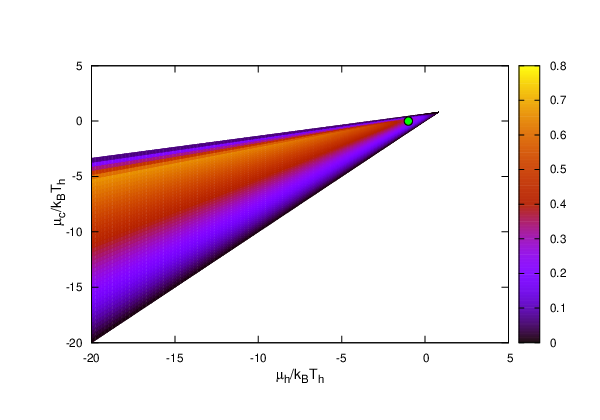
When operating for a finite time, the quantities and , and hence also the stochastic efficiency , are different from one run to another [1]. One may wonder about thermodynamic implications for the probability distribution of . In a recent paper [2] (see also [3, 4]), the following remarkable result was derived: in a non-macroscopic machine running for long but finite times, the reversible efficiency is least probable (in the sense of large deviations [5]). This property is based on the generalisation of the second law of thermodynamics for small systems, the so-called fluctuation theorem, and parallels the derivation of Carnot or reversible efficiency of macroscopic machines. The simplest illustration is the work to work transformation by a Brownian particle subjected to competing external forces [2]. The reversible efficiency is here . Both work components are Gaussian and the explicit analytic result is available for the probability distribution of the stochastic efficiency [6] and its large deviation function [2]. In this letter, we calculate the stochastic efficiency for the effusion engine, which is, as we argue below, the simplest possible construction of a thermal machine. The analytic expression for the large deviation properties of work and heat can be obtained, as well as that for the efficiency apart from a final step involving a parametric elimination. Furthermore, the finite time regime with the approach to the large deviation limit and the deviations from the Gaussian regime can be studied in detail. All the results are of course in agreement with the universal predictions from [2].
The simplicity of the effusion engine stems from the fact that there is no auxiliary engine part that transfers the energy. Furthermore, the crossing of the particles is described by basic Poisson statistics. To illustrate the calculations and to incidentally show how the Carnot efficiency can be recovered, we first consider effusion operating with a filter, such that only particles with energies in a small window are allowed to cross. The number of particles leaving the hot reservoir during a time is described by a Poisson distribution:
| (2) |
with the crossing rate prescribed by kinetic theory:
| (3) |
Here we introduced the average escape time for a particle in the absence of an energy filter:
| (4) |
and is the surface area of the effusion hole. A similar result holds for the crossing of particles coming from the cold reservoir by formally replacing the subscript by and by . Since the crossings are independent from each other, we find by convolution that the probability to have a net transfer of particles, is given by:
| (5) |
This is nothing but the probability distribution for a biased continuous-time random walk with stepping rates and . The so-called large deviation function describes the asymptotic probability for observing an empirical particle flux :
| (6) |
It is found from Eq. (5) by Stirling’s formula:
| (7) |
Note that in the presence of a single energy filter, the net energy transfer and net particle transfer become ”strongly coupled”: . Also work and heat are proportional to each other. Hence, even while both and fluctuate through their dependence on , the efficiency, , remains constant. Since in this case , the second law requires . It is revealing to show how Carnot efficiency can be reached in this case [7, 8]. The crucial condition is that one operates under equilibrium conditions, i.e., the Maxwell-Boltzmann density of particles of energy has to be the same in both compartments: . This indeed yields for an ideal gas ( apart from an additive constant): (see Supplemental Material). Note that equilibrium is reached even though density, chemical potential and temperature need not be the same in both compartments.
To obtain a nontrivial result for the probability distribution of the efficiency, we consider next effusion through two separate windows, selective for energies and , respectively. The discrete amounts of work and heat, produced upon a net transfer (from hot to cold) of particles through window and particles through window , are obviously given by:
| (8) |
with and the transported heat per particle leaving the hot reservoir via filter and , respectively :
| (9) |
Since the transport through both filters is statistically independent, the joint probability for work and heat is given by the following convolution:
| (10) | |||||
being the probability for a net transfer of particles through the -th filter after a time , . It is given by Eq. (5) with and replaced by the corresponding values for filter (we used the same for both filters). Considering the large time limit, the heat and work fluxes and are characterised by the following large deviation function:
where is the large deviation function of the net particle flux through the -th filter, , given by (7) with the appropriate values of the rates and .
Turning to the efficiency , we note that its probability distribution:
| (12) | |||||
can be obtained for any finite time by combination with Eq.(10), cf. Fig. 2. For the corresponding large deviation function , one finds:


| (13) | |||||
with
| (14) |
We have used the contraction principle [5], expressing the fact that a given value of is realised by the most likely values of and for which . The above minimization involves a transcendental equation (see Supplemental Material), requiring a numerical solution. The resulting large deviation function has the familiar shape [2], with a zero in , a maximum at Carnot efficiency, and equal asymptotes for , cf. Fig. 2.


One can repeat the above calculation for effusion without energy filters (see Supplemental Material). Results are shown in Fig. 3. Note in Fig. 3 the ”fine structure” appearing for small times around , due to the fact that very few particles will cross. The observed minimum of around zero is for example due to the very unlikely single particle crossing with high energy, the latter being required to obtain a small value of .
We turn to a discussion of the salient features and implications of our analysis. The first conclusion is that all the predictions of the general theory [2] are verified, and in particular the generic properties of the large deviation function . Second, both the Gaussian regime and the strongly non-Gaussian regime can be easily observed, as well as other special limits such as the ”strong coupling” limit or the limit to ”reversibility”. Third, the minimum of the probability or the maximum of the large deviation function at Carnot efficiency can be made very pronounced, rendering the most striking feature, the minimum at Carnot efficiency, easy to observe. Fourth, an accurate estimation of the large deviation function is possible by extrapolating the results from finite time, as is shown in the insets of Figs. 2 and 3. Fifth, even for relatively short times (less than sec) and with rather small statistics ( samples), the minimum of the the probability can clearly be identified, as can be seen in Fig. 4. Sixth, the probability distribution for the efficiency of effusion displays long tails, similar to the one observed in the Gaussian scenario [6]. This appears to be a generic result. Indeed it follows from (12) that:
| (15) |
provided has a smooth behavior around and the integral converges.

Last but not least, we discuss the experimental setting for an effusion engine displaying the salient features of stochastic efficiency. To obtain a sharp minimum of at Carnot efficiency, a large value of is required. One way to do so in the two filter effusion engine is by considering and . This region is described by (see Supplemental Material). With this condition in mind, we have performed simulations for the stochastic efficiency of an effusion engine operating with Helium gas. In Fig. 4, we represent (window ) obtained by , and samplings. The minimum in the vicinity of Carnot efficiency is clearly visible, even at these very short times.
In conclusion, effusion as a thermal engine displays all the key features of stochastic efficiency. The model combines conceptual simplicity with analytic tractability and experimental relevance. It is generic for the case in which transitions are ruled by Poisson statistics, such as in Kramers’ escape over a potential barrier, or for transitions ruled by a chemical reaction.
References
- [1] B. Cleuren, C. Van den Broeck, and R. Kawai, Physical Review E 74, 021117 (2006).
- [2] G. Verley, T. Willaert, C. Van den Broeck, and M. Esposito, Nature Communications 5 (2014a).
- [3] T. R. Gingrich, G. M. Rotskoff, S. Vaikuntanathan, and P. L. Geissler, New Journal of Physics 16, 102003 (2014).
- [4] G. Verley, T. Willaert, C. Van den Broeck, and M. Esposito, arXiv:1409.3514 (2014b).
- [5] H. Touchette, Physics Reports 478, 1 (2009).
- [6] M. Polettini, G. Verley, and M. Esposito, arXiv:1409.4716 (2014).
- [7] T. Humphrey and H. Linke, Physical Review Letters 94, 096601 (2005).
- [8] C. Van den Broeck, Advances in Chemical Physics 135, 189 (2007).