Probing short-lived fluctuations in hadrons and nuclei
Abstract
We develop a picture of dipole-nucleus (namely dilute-dense) and dipole-dipole (dilute-dilute) scattering in the high-energy regime based on the analysis of the fluctuations in the quantum evolution. We emphasize the difference in the nature of the fluctuations probed in these two processes respectively, which, interestingly enough, leads to observable differences in the scattering amplitude profiles.
Keywords:
Quantum chromodynamics, high-energy scattering, hadronic cross sections, parton evolution, color dipole model, fluctuationsClassification:
12.38.-t,13.85.-tThis paper introduces and summarizes the results recently published in Ref. Mueller and Munier (2014a), from a less technical viewpoint (see Ref. Munier (2014) for a complementary presentation), and with illustrations from numerical simulations (see Figs. 2 and 3 below). Our goal is to understand the qualitative properties of the short-lived and short-distance (with respect to ) quantum fluctuations, namely the ones that are probed most efficiently in deep-inelastic scattering experiments in the small- regime, or in observables in proton-proton and proton-nucleus scattering whose cross sections may be related to dipole amplitudes (see e.g. Ref. Mueller and Munier (2012)). (A recent general review of high-energy QCD can be found in Ref. Kovchegov and Levin (2012)).
We shall first describe qualitatively the scattering of two color dipoles and of a dipole off a nucleus, before turning to an analysis of the quantum fluctuations. We shall eventually review the most striking quantitative prediction derived from our discussion.
Our picture relies on the well-known color dipole model Mueller (1994), which describes, in the framework of perturbative quantum chromodynamics, how the quantum state of a hadron builds up from a cascade of dipole splittings.
1 Picture of the interaction of a small dipole with QCD matter
1.1 Scattering of a dipole off a dilute target and off a dense target
We start with the scattering of two color dipoles (concretely, e.g. two quark-antiquark pairs) of respective transverse sizes and with the ordering .
At low energy, the forward elastic scattering amplitude of the dipoles consists in the exchange of a pair of gluons. Since the dipoles are colorless, this exchange can take place only if their sizes are comparable (on a logarithmic scale), and if the scattering occurs at coinciding impact parameters. Once these conditions are fulfilled, the cross section is parametrically proportional to .
Let us go to larger center-of-mass
energies
by boosting the small dipole to the
rapidity .
The most probable Fock state at the time
of the interaction is then a dense state of gluons, which
may be represented by a set of dipoles Mueller (1994)
(see the sketch in Fig. 1a).
The amplitude is now enhanced by the number of
these dipoles which have a size of the order of .
We may define a “one-event amplitude” ,
which is related to
the probability that gluons are exchanged between one given realization
of the dipole evolution and the target dipole.
If denotes the number of dipoles in a given realization
of the evolution up to rapidity of size , starting with
a dipole of size , then
,
where it is understood that the impact parameters
of the dipoles which scatter
need to coincide
(up to a distance of order of the smallest size).
Of course, the dipole number fluctuates from event to event,
and so does
.
The physical amplitude measured in an experiment is proportional to
the average of the latter over events, namely over
realizations of the dipole evolution.
We conclude that the scattering of two dipoles of respective sizes
and probes the
density of gluons of transverse size , at a given
impact parameter, in typical quantum
fluctuations of a source dipole of size
appearing in the quantum evolution over the rapidity .

|

|
|---|---|
| (a) | (b) |
We turn to the case in which instead of the dipole of size , the target consists in a large nucleus. At low energy, the dipole now scatters through multiple gluon exchanges since the nucleus is dense. The Glauber-Mueller summation of the latter implemented in the McLerran-Venugopalan model McLerran and Venugopalan (1994) gives the scattering amplitude in the form . A new momentum scale is generated: It is the saturation momentum of the nucleus, and grows with the nucleus mass number like . This amplitude may actually be approximated by a Heaviside function:11 1 This statement relies on the fact that the exponential in the McLerran-Venugopalan formula is “steep”, in some sense. The full argument specifies what “steep” means, which is not completely straightforward, see the discussion in Ref. Mueller and Munier (2014a). . This has the advantage of simplifying the interpretation of the scattering of the evolved dipole with the nucleus.
If one increases the center-of-mass energy by boosting the dipole, then at the time of the interaction, in each event, the nucleus “sees” a set of dipoles. The interaction takes place if and only if at least one dipole in this set has a size larger than the inverse saturation momentum. Hence if at least one of the dipoles in the evolution is larger than , or 0 else. The cross section that is measured in an experiment by counting events (which technically is an averaging of over the events) is thus the probability that at least one dipole in the Fock state of the source dipole evolved to the time of the interaction has a size larger than (see Fig. 1b). Hence, while dipole-dipole scattering probes the bulk of the quantum state, the scattering of a dipole of size with a nucleus is sensitive to the probability distribution of the size of the largest fluctuation generated in the quantum evolution of the dipole, namely, in a mathematical language, to the statistics of extremes.
1.2 Rapidity evolution of a dipole
We have just argued that scattering amplitudes can be thought of as probes of the quantum fluctuations of the dipole. The latter are best pictured with the help of the color dipole model. We shall now describe the way how these fluctuations build up (see Ref. Mueller and Munier (2014b) for an extensive discussion), in order to arrive at a model that leads to quantitative predictions for the scattering amplitudes.
In these matters, useful intuition can be gained from numerical
implementations of the dipole model in the
form of a Monte Carlo event generator Salam (1997).
Therefore, we shall illustrate our arguments with the help
of simulations of the toy model constructed
in Ref. Munier et al. (2008).
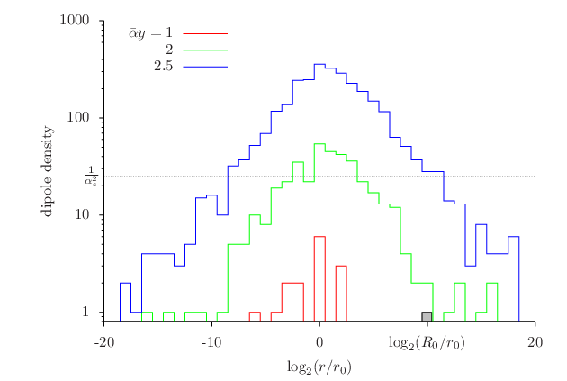
The quantum evolution of the dipole proceeds through successive independent splittings , with rate per unit rapidity given by the probability distribution , where is the size vector of the initial dipole, and are the size vectors of the offspring, and . The stochastic process of dipole evolution is a branching diffusion. Indeed, if one looks at the distribution of the log of the dipole sizes at a given impact parameter, it has a Gaussian-like shape growing exponentially with the rapidity, see Fig. 2a. The stochasticity has a strong effect wherever the number of dipoles is of order unity, namely either in the beginning of the evolution (for low rapidities), or at the edges of the distribution. Elsewhere, in the bulk of the distribution, the law of large numbers applies, and therefore, the rapidity evolution of the dipole density is nearly deterministic.
According to these observations,
in Ref. Mueller and Munier (2014a), we conjectured that there are
essentially two types of fluctuations: The “front fluctuations” that
come from the early stages of the evolution,
and the “tip fluctuations” occurring throughout the
evolution in the regions in which the dipole density is low.
Both kinds of fluctuations shift the distribution
of dipoles towards larger sizes,
by say and respectively, in logarithmic scale.
We conjectured that the latter random variables are distributed exponentially,
and ,
where is a number determined by the eigenvalues of
the BFKL kernel.
|

|
|---|---|
| (a) | (b) |
The way how the scattering probes the quantum evolution is represented in
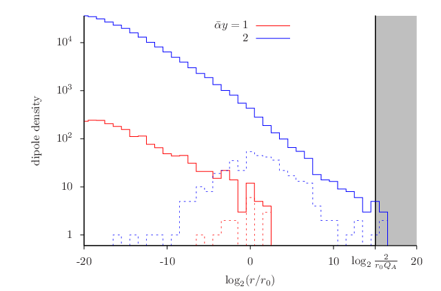
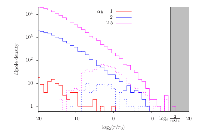
Figs. 2 and 3.
Since the number of dipoles grows exponentially with the rapidity,
would at some point violate unitarity if the formula for
applied without restrictions. But we know that saturation effects (for example
rescatterings, gluon recombination…) may occur in the course of the evolution
so that the effective number of dipoles does never grow
larger than
(see Fig. 2b).
These saturation effects are crucial in the dipole case, since
the scattering is sensitive to the shape of the bulk
of the distribution of the quantum fluctuations.
They make the averaging over events nontrivial.22
2
In the dipole case, only the front fluctuations have a
significant effect on the amplitude.
This holds true
for low enough rapidities, namely ;
see e.g. Munier (2009) for a discussion
of how this scale comes about.
|
|
|---|---|
| (a) | (b) |
In the nucleus case (Fig. 3),
it is the size of the largest dipole
which determines the shape of the amplitude. Therefore, both front and
tip fluctuations must be taken into account. On the other hand, the shape
of the amplitude is less sensitive to saturation effects
in the dipole evolution, at variance
with the dipole case, at least for rapidities parametrically
less than .
In the regions in which the dipole distribution is deterministic, the latter essentially has the shape near the large-size tip of the distribution, where is the saturation momentum. Here, may be thought of as the smallest dipole size for which, in a typical event, there is an overlap of the dipole number distribution with the target. The expression of is given in Ref. Mueller and Munier (2014a).
2 Phenomenological predictions
From our model for the fluctuations, an elementary calculation leads to the shape of the scattering amplitudes in the dipole-dipole and dipole-nucleus cases:
The calculation simply averages the amplitude over events, assuming that the stochasticity is fully captured by the distribution of the random variables and , see again Ref. Mueller and Munier (2014a) for all details and more results.
The fact that the power of the logarithmic prefactor be different in the dipole-dipole and dipole-nucleus cases is our main result.
References
- Mueller and Munier (2014a) A. Mueller, and S. Munier, Phys.Lett. B737, 303–310 (2014a), 1405.3131.
- Munier (2014) S. Munier, Proceedings of the PANIC2014 conference (2014), 1410.5656.
- Mueller and Munier (2012) A. Mueller, and S. Munier, Nucl.Phys. A893, 43–86 (2012), 1206.1333.
- Kovchegov and Levin (2012) Y. Kovchegov, and E. Levin, Quantum Chromodynamics at High Energy, Cambridge Monographs on Particle Physics, Nuclear Physics and Cosmology, Cambridge University Press, 2012, ISBN 9780521112574, URL http://books.google.fr/books?id=f2nHp-NeW6UC.
- Mueller (1994) A. H. Mueller, Nucl.Phys. B415, 373–385 (1994).
- McLerran and Venugopalan (1994) L. D. McLerran, and R. Venugopalan, Phys.Rev. D49, 2233–2241 (1994), hep-ph/9309289.
- Mueller and Munier (2014b) A. Mueller, and S. Munier, Phys.Rev. E90, 042143 (2014b), 1404.5500.
- Salam (1997) G. Salam, Comput.Phys.Commun. 105, 62–76 (1997), hep-ph/9601220.
- Munier et al. (2008) S. Munier, G. Salam, and G. Soyez, Phys.Rev. D78, 054009 (2008), 0807.2870.
- Munier (2009) S. Munier, Phys.Rept. 473, 1–49 (2009), 0901.2823.