Dark Energy and Equation of State Oscillations with Collisional Matter Fluid in Exponential Modified Gravity

In principle an $F(R)$ gravity model has to pass a series of serious tests in order it can be considered a viable model. The constraints put by these tests are coming both from local astrophysical data and also from global, at a cosmological level, considerations, see for example [7, 8, 9, 10, 11, 14, 15, 16, 17, 18, 19, 20, 21, 22, 23, 24, 25, 26] and related references therein. In this paper we shall consider a viable exponential model, firstly studied in [23] by Cognola, Elizalde et al., which passes all the viability tests and also provides a very elegant theoretical framework for explaining late time acceleration and also inflation, at the early stages of the universe’s evolution, mimicking the $\Lambda$CDM model at large curvature values. For studies on exponential models, the reader is referred to [23, 24, 45, 46, 47, 48]. The model is described by the following $F(R)$ function,

$$F(R)=R-2\Lambda\left(1-e^{\frac{R}{b\Lambda}}\right)$$

(8)

with $\Lambda$ being the cosmological constant corresponding to present time, which is equal to $\Lambda\simeq 11.89$eV² and $b$ is a free positive parameter which is assumed to be $b\simeq 1$ (we adopt the numerical values of reference [45]). Regardless the good viability properties of the model (8), there are some complications that arise in the process of the cosmological evolution and particularly during the matter domination era. Particularly, the higher derivatives of the Hubble parameter diverge, an issue that originates from the dark energy oscillations during the matter phase [44, 45, 47]. In fact for large values of the redshift, there occur high frequency dark energy oscillations, and also the derivatives of the dark energy density, denoted as $\rho_{DE}$, take large values, which leave this imprint in the dark energy equation of state parameter $\omega_{DE}$. Actually, the dark energy oscillations become more pronounced (higher frequency) in $F(R)$ modified gravity models that mimic more the $\Lambda$CDM model, which practically speaking occurs when $F^{\prime\prime}(R)$ is close to zero. Thus our fundamental function of the exponential model (8) to correct Einstein’s gravity in the small curvature regime, causes undesirable features in the high curvature regime. A way out of this is offered by directly modifying the $F(R)$ gravity Lagrangian, in order to stabilize dark energy oscillations, in such a way so that the frequency of the oscillations becomes constant [45, 47]. A consistent modification was proposed in [45], so that the curvature corrected $F(R)$ Lagrangian reads,

$$F(R)=R-2\Lambda\left(1-e^{\frac{R}{b\Lambda}}\right)-\tilde{\gamma}\Lambda\left(\frac{R}{3\tilde{m}^{2}}\right)^{1/3}$$

(9)

with $\Lambda=7.93\tilde{m}^{2}$ and $\tilde{\gamma}=1/1000$ [45]. The addition of the curvature correction stabilizes the dark energy oscillations while keeping all the viability features of the model intact. For example the Minkowski spacetime still is the flat space solution and the effects of the curvature correction vanish in the de-Sitter epoch, provided $\tilde{\gamma}\ll(\tilde{m}^{2}/\Lambda)^{1/3}$, which obviously is satisfied for the adopted value of $\tilde{\gamma}$.

The detailed description of a perfect matter fluid with interactions was given in [42, 43] and reference therein (see also [41]). It worths recalling in brief, the basic features which we shall use in this article. The basic assumption to be made is that the collisional matter has a total mass-energy density, denoted as $\varepsilon_{m}$, which receives two contributions in it’s functional form and reads,

$$\varepsilon_{m}=\rho_{m}+\rho_{m}\Pi$$

(10)

In the expression above, $\rho_{m}$ stands for the rest mass density which remains unaffected by the internal motions of the gravitational cosmic fluid and the part containing the potential energy $\Pi$, is what renders the matter fluid collisional [42, 43]. The collisional matter is considered to be a prefect fluid with equation of state,

$$p_{m}=w\rho_{m}$$

(11)

with the equation of state parameter taking values $0<w<1$. The potential energy density is assumed to be of the form [42, 43],

$$\Pi=\Pi_{0}+w\ln(\frac{\rho_{m}}{\rho_{m}^{(0)}})$$

(12)

with $\rho_{m}^{(0)}$ and $\Pi_{0}$ denoting the present values of the motion invariant mass energy density and of the potential energy, respectively. Hence, the total energy density of the gravitational fluid is equal to,

$$\varepsilon_{m}=\rho_{m}\Big[1+\Pi_{0}+w\ln(\frac{\rho_{m}}{\rho_{m}^{(0)}})\Big]$$

(13)

In addition and due to the continuity equation for the collisional matter fluid (see the book of Fock [43], pages 90-93), the continuity equation of the gravitational fluid in a spatially flat FRW metric takes the following form,

$$\dot{\varepsilon}_{m}+3\frac{\dot{a}}{a}(\varepsilon_{m}+p_{m})=0$$

(14)

which leads to [42],

$$\rho_{m}=\rho_{m}^{(0)}\big(\frac{a_{0}}{a}\big)^{3}$$

(15)

with $a$ and $a_{0}$ denoting the scale factor and it’s present value respectively. Finally the value of $\Pi_{0}$ is equal to [42],

$$\Pi_{0}=\Big(\frac{1}{\Omega_{M}}-1\Big)$$

(16)

which we shall use in our numerical calculations. In the next section we shall go through the equations of cosmological evolution and see in detail how these are modified in the presence of a collisional matter fluid with total mass-energy density given by relation (13).

Our basic intention and core subject of this section, is to study the cosmological evolution of a universe filled with collisional matter and radiation, with special emphasis in the redshift region which corresponds to matter domination and later. This is in order to study the dark energy oscillations during this era, which as we already mentioned in the previous sections, can have a significant value during this era and at low redshifts in general. We shall express the quantities entering the FRW equations in terms of the redshift parameter $z=1/a-1$ and also use new variables, appropriate for the study of dark energy oscillations. We shall perform a numerical analysis of the modified FRW equations for the type of collisional matter described in the previous section, and thoroughly study the behavior of the dark energy density $\Omega_{DE}(z)$, the modified Hubble parameter, $H(z)$ and of the effective equation of state parameter $\omega_{eff}$, which we re-express later in terms of the new variables we shall introduce. For the numerical analysis, we shall take into account values of the redshift $z\leq 10$, which covers the last stages of the matter domination era, which started at approximately $z\sim 3000$ and is considered to end at $z\simeq 3$ (this can vary from model to model). After that the late time acceleration era starts. The motivation for us to use the redshift as our central parameter of our analysis comes from the fact that, the cosmological distances in standard cosmology are determined by using standard candles as references, such as TypeIa supernovae or Gamma Ray Bursts (GRB hereafter wherever used). The TypeIa supernovae correspond to a redshift with values between $0<z<1.7$. In addition, GRBs are visible in much more higher redshifts, up to $z=6$, which corresponds to the late stages of the matter domination era. This is why we shall use values of the redshift with $0\leq z\leq 10$, in order to take into account future observational data coming from GRBs corresponding to high redshifts with $z\geq 6$.

In order to proceed in the description of the cosmological evolution, we rewrite the cosmological equations in a specific form. Particularly, the FRW equations of motion (4) can be written in the following form,

		$\displaystyle 3F^{\prime}H^{2}=k^{2}\rho_{matt}+\frac{1}{2}(F^{\prime}R-F)-3H\dot{F^{\prime}}$		(17)
		$\displaystyle-2F^{\prime}\dot{H}=k^{2}\left(\rho_{matt}+P_{matt}\right)+\ddot{F}-H\dot{F}$

with $\rho_{matt}$ being the total mass-energy density containing all the matter fluids. In the present case the matter fluids we shall take into account consist of collisional matter and relativistic matter (radiation), so $\rho_{matt}$ is in our case,

$$\rho_{matt}=\varepsilon_{m}+\rho_{r}^{(0)}a^{-4}$$

(18)

and by taking into account relations (13) and (15), equation (18) becomes,

$$\rho_{matt}=\rho_{m}^{(0)}a^{-3}\Big[1+\Pi_{0}+3w\ln(a)\Big]+\rho_{r}^{(0)}a^{-4}$$

(19)

In addition, $P_{matt}$ is the corresponding total pressure corresponding to all the matter fluids. The first equation of the FRW equations in relation (17) can be written as,

$$H^{2}-(F^{\prime}-1)\left(H\frac{\mathrm{d}H}{\mathrm{d}\ln{a}}+H^{2}\right)+\frac{1}{6}(F-R)+H^{2}F^{\prime\prime}\frac{\mathrm{d}R}{\mathrm{d}\ln{a}}=\frac{\rho_{matt}}{3},$$

(20)

where $R$ is the Ricci scalar which for the purposes of this paper, can be written as,

$$R=12H^{2}+6H\frac{\mathrm{d}H}{\mathrm{d}\ln{a}},$$

(21)

In order to provide general formulas that hold true for any type of collisional matter, we shall assume that the total matter-energy density takes the following general form,

$$\rho_{matt}=\rho_{m}^{(0)}g(a)+\rho_{r}^{(0)}a^{-4}=\rho_{m}^{(0)}\left(g(a)+\chi a^{-4}\right),$$

(22)

with $\rho_{m}^{(0)}$ and $\rho_{r}^{(0)}=\chi\rho_{m}^{(0)}$ being the present values of the mass-energy densities of matter and radiation respectively, and $\chi\simeq 3.1\times 10^{-4}$ being defined as the ratio $\rho_{r}^{(0)}/\rho_{m}^{(0)}$. So practically, the collisional nature of the non-relativistic matter is described by the function $g(a)$, which in the case of collisional matter described in the previous section, this is equal to,

$$g(a)=a^{-3}\Big[1+\Pi_{0}-3w\ln(a)\Big]$$

(23)

In order to consistently describe the dark energy oscillations, we re-express the cosmological equations (20) in terms of new parameters which have vanishing values at the high redshift limits, where the $F(R)$ modifications are negligible [17],

	$\displaystyle y_{H}$	$\displaystyle\equiv\frac{\rho_{DE}}{\rho_{m}^{(0)}}\frac{H^{2}}{\tilde{m}^{2}}-g(a)-\chi a^{-4}$		(24a)
	$\displaystyle y_{R}$	$\displaystyle\equiv\frac{R}{\tilde{m}^{2}}-\frac{\mathrm{d}g(a)}{\mathrm{d}\ln{a}}$		(24b)

with $\rho_{DE}$ the energy density of dark energy. So the new quantity which quantifies the cosmological evolution is, $y_{H}(z)$, which is the scaled dark energy density, and scaled by the factor $\rho_{m}^{(0)}$. Dividing the equations (20) by $\tilde{m}^{2}$, and upon using,

$$\frac{H^{2}}{\tilde{m}^{2}}-\frac{\rho_{M}}{2\tilde{m}^{2}}=\frac{H^{2}}{\tilde{m}^{2}}-g(a)-\chi a^{-4}=y_{H}$$

(25)

from (24a), we solve the resulting expression with respect to $\frac{1}{\tilde{m}^{2}}\frac{dR}{d\ln{a}}$. The final result is,

$$\frac{1}{\tilde{m}^{2}}\frac{\mathrm{d}R}{\mathrm{d}\ln{a}}=\left[-y_{H}+(F^{\prime}-1)(\frac{H}{\tilde{m}^{2}}\frac{\mathrm{d}H}{\mathrm{d}\ln{a}}+\frac{H^{2}}{\tilde{m}^{2}})-\frac{1}{6\tilde{m}^{2}}(F-R)\right]\frac{1}{H^{2}F^{\prime\prime}}$$

(26)

Upon differentiation of relation (24b), with respect to $\ln{a}$ we get,

$$\frac{\mathrm{d}R}{\mathrm{d}\ln{a}}=\frac{1}{\tilde{m}^{2}}\frac{\mathrm{d}R}{\mathrm{d}\ln{a}}-\frac{\mathrm{d}^{2}g(a)}{\mathrm{d}\ln{a}^{2}},$$

(27)

in which we substitute (26),

$$\frac{\mathrm{d}y_{R}}{\mathrm{d}\ln{a}}=-\frac{\mathrm{d}^{2}g(a)}{\mathrm{d}\ln{a}^{2}}+\left[-y_{H}+(F^{\prime}-1)(\frac{H}{\tilde{m}^{2}}\frac{\mathrm{d}H}{\mathrm{d}\ln{a}}+\frac{H^{2}}{\tilde{m}^{2}})-\frac{1}{6\tilde{m}^{2}}(F-R)\right]\frac{1}{H^{2}F^{\prime\prime}}$$

(28)

Upon differentiation of (24a) with respect to $\ln{a}$, we get,

	$\displaystyle\frac{\mathrm{d}y_{H}}{\mathrm{d}\ln{a}}$	$\displaystyle=$	$\displaystyle 2\frac{H}{\tilde{m}^{2}}\frac{\mathrm{d}H}{\mathrm{d}\ln{a}}-\frac{\mathrm{d}g(a)}{\mathrm{d}\ln{a}}+4\chi a^{-4}$
	$\displaystyle\Rightarrow\frac{H}{\tilde{m}^{2}}\frac{\mathrm{d}H}{\mathrm{d}\ln{a}}$	$\displaystyle=$	$\displaystyle\frac{1}{2}\frac{\mathrm{d}y_{H}}{\mathrm{d}\ln{a}}+\frac{1}{2}\frac{\mathrm{d}g(a)}{\mathrm{d}\ln{a}}-2\chi a^{-4}$
	$\displaystyle\Rightarrow\frac{H}{\tilde{m}^{2}}\frac{\mathrm{d}H}{\mathrm{d}\ln{a}}+\frac{H^{2}}{\tilde{m}^{2}}$	$\displaystyle=$	$\displaystyle\frac{1}{2}\frac{\mathrm{d}y_{H}}{\mathrm{d}\ln{a}}+\frac{1}{2}\frac{\mathrm{d}g(a)}{\mathrm{d}\ln{a}}+y_{H}+g(a)-\chi a^{-4},$		(29)

where we made use of relation (24a). Combining equations (29) and (28), we get the following expression,

	$\displaystyle\frac{\mathrm{d}y_{R}}{\mathrm{d}\ln{a}}$	$\displaystyle=$	$\displaystyle-\frac{\mathrm{d}^{2}g(a)}{\mathrm{d}\ln{a}^{2}}+\left[-y_{H}+(F^{\prime}-1)\left(\frac{1}{2}\frac{\mathrm{d}y_{H}}{\mathrm{d}\ln{a}}+\frac{1}{2}\frac{\mathrm{d}g(a)}{\mathrm{d}\ln{a}}+y_{H}+g(a)-\chi a^{-4}\right)\right.$		(30)
			$\displaystyle\left.-\frac{1}{6\tilde{m}^{2}}(F-R)\right]\frac{1}{\tilde{m}^{2}F^{\prime\prime}(y_{H}+g(a)+\chi a^{-4})}.$

Differentiating relation (26) with respect to $\ln{a}$, results to,

$$\frac{\mathrm{d}y_{H}}{\ln{a}}=\frac{2H}{\tilde{m}^{2}}\frac{\mathrm{d}H}{\mathrm{d}\ln{a}}-\frac{\mathrm{d}g(a)}{\mathrm{d}\ln{a}}+4\chi a^{-4}.$$

(31)

From (21) and (24a) we get,

$$\frac{2H}{\tilde{m}^{2}}\frac{\mathrm{d}H}{\ln{a}}=\frac{R}{3\tilde{m}^{2}}-\frac{4H^{2}}{\tilde{m}^{2}}=\frac{R}{3\tilde{m}^{2}}-4y_{H}-4g(a)-4\chi a^{-4},$$

(32)

so relation (31) becomes,

	$\displaystyle\frac{\mathrm{d}y_{H}}{\mathrm{d}\ln{a}}$	$\displaystyle=$	$\displaystyle\frac{R}{3\tilde{m}^{2}}-\frac{\mathrm{d}g(a)}{\mathrm{d}\ln{a}}-4y_{H}-4g(a)$		(33)
		$\displaystyle=$	$\displaystyle\frac{y_{R}}{3}-4y_{H}-\frac{2\mathrm{d}g(a)}{3\mathrm{d}\ln{a}}-4g(a)$

and in addition the Ricci scalar can be written as,

$$R=3\tilde{m}^{2}\left(4y_{H}+4g(a)+\frac{\mathrm{d}y_{H}}{\mathrm{d}\ln{a}}+\frac{\mathrm{d}g(a)}{\mathrm{d}\ln{a}}\right)$$

(34)

Upon differentiation of relation (33) with respect to $\ln{a}$,

$$\frac{\mathrm{d}^{2}y_{H}}{\mathrm{d}\ln{a}^{2}}=\frac{\mathrm{d}y_{R}}{3\mathrm{d}\ln{a}}-\frac{4\mathrm{d}y_{H}}{\mathrm{d}\ln{a}}-\frac{2}{3}\frac{\mathrm{d}^{2}g(a)}{\mathrm{d}\ln{a}^{2}}-4\frac{\mathrm{d}g(a)}{\mathrm{d}\ln{a}}$$

and by making use of relation (30), we obtain,

	$\displaystyle\frac{\mathrm{d}^{2}y_{H}}{\mathrm{d}\ln{a}^{2}}+\left(4+\frac{1-F^{\prime}}{6\tilde{m}^{2}F^{\prime\prime}(y_{H}+g(a)+\chi a^{-4})}\right)\frac{\mathrm{d}y_{H}}{\mathrm{d}\ln{a}}+\left(\frac{2-F^{\prime}}{3\tilde{m}^{2}F^{\prime\prime}(y_{H}+g(a)+\chi a^{-4})}\right)y_{H}$
	$\displaystyle+\left(\frac{\mathrm{d}^{2}g(a)}{\mathrm{d}\ln{a}^{2}}+4\frac{\mathrm{d}g(a)}{\mathrm{d}\ln{a}}+\frac{(1-F^{\prime})\left(3\frac{\mathrm{d}g(a)}{\mathrm{d}\ln{a}}+6g(a)-6\chi a^{-4}\right)+\frac{F-R}{\tilde{m}^{2}}}{18\tilde{m}^{2}F^{\prime\prime}(y_{H}+g(a)+\chi a^{-4})}\right)=0$		(35)

Finally we express all quantities as functions of the redshift $z$, and order to do that, we shall make use of the following expressions,

	$\displaystyle\frac{\mathrm{d}}{\mathrm{d}\ln{a}}$	$\displaystyle=-(z+1)\frac{\mathrm{d}}{\mathrm{d}z},$		(36a)
	$\displaystyle\frac{\mathrm{d}^{2}}{\mathrm{d}\ln{a}^{2}}$	$\displaystyle=(z+1)\frac{\mathrm{d}}{\mathrm{d}z}+(z+1)^{2}\frac{\mathrm{d}^{2}}{\mathrm{d}z^{2}}.$		(36b)

Then, by applying the above formulas in relation (35), we obtain the following final form of the differential equation that describes the cosmological evolution of the universe filled with radiation and collisional matter,

	$\displaystyle\frac{\mathrm{d}^{2}y_{H}}{\mathrm{d}z^{2}}+\frac{1}{(z+1)}\left(-3-\frac{F^{\prime}(R)}{6\tilde{m}^{2}F^{\prime\prime}(R)(y_{H}+g(z)+\chi(z+1)^{4})}\right)\frac{\mathrm{d}y_{H}}{\mathrm{d}z}$
	$\displaystyle+\frac{1}{(z+1)^{2}}\frac{1-F^{\prime}(R)}{3\tilde{m}^{2}F^{\prime\prime}(R)(y_{H}+g(Z)+\chi(z+1)^{4})}y_{H}+\left(\frac{\mathrm{d}^{2}g(z)}{\mathrm{d}z^{2}}-\frac{3}{(z+1)}\frac{\mathrm{d}g(z)}{\mathrm{d}z}\right.$
	$\displaystyle\left.-\frac{1}{(z+1)}\frac{F^{\prime}(R)\left(-(z+1)\frac{\mathrm{d}g(z)}{\mathrm{d}z}+2g(z)-2\chi(z+1)^{4}\right)+\frac{F}{3\tilde{m}^{2}}}{6\tilde{m}^{2}F^{\prime\prime}(R)(y_{H}-g(z)+\chi(z+1)^{4})}\right)=0$		(37)

which is a second order differential equation in terms of the scaled dark energy $y_{H}$. In the rest of this section we solve numerically this equation for the matter profile $g(a)$ given in relation (23) and compare the dark energy oscillations and the cosmological evolutions of collisional matter in comparison to the non-collisional one. It worths to present briefly the set of initial conditions and also the values of the various parameters we shall use. Specifically, the present value of the matter density is $\Omega_{M}=0.279$, the equation of state parameter of collisional matter shall be assumed to have two different values, $w=0.1$ and $w=0.7$, and the initial conditions are taken to be identical to those used in reference [45],

$$y_{H}(z)\mid_{z=z_{f}}=\frac{\Lambda}{3\tilde{m}^{2}}\left(1+\frac{z_{f}+1}{1000}\right),{\,}{\,}{\,}y_{H}^{\prime}(z)\mid_{z=z_{f}}=\frac{\Lambda}{3\tilde{m}^{2}}\frac{1}{1000}$$

(38)

with $z_{f}=10$ and $\Lambda$, $\tilde{m}^{2}$ being defined in the previous sections.

We start off with the comparison of the function $y_{H}(z)$ for collisional and non-collisional matter and in Fig. 1 we present of the numerical analysis we performed, for $w=0.1$ (left) and $w=0.7$ (right) with the blue line corresponding to collisional matter with $g(a)$ given in (23) and the red line corresponding to non-collisional matter ($g(a)=a^{-3}$).

As we can see, the behavior of the scaled dark energy density $y_{H}(z)=\frac{\rho_{DE}}{\rho_{m}^{(0)}}$ for collisional matter is more oscillatory in reference to non-collisional matter, and this phenomenon gets more pronounced as $w$ increases. The latter is rather normal, because the more $w$ approaches the value zero, the collisional nature of matter disappears. In reference to dark energy oscillations, we shall compare the dark energy equation of state parameter $\omega_{DE}=P_{DE}/\rho_{DE}$ for collisional and non-collisional matter for various $w$ values. It worths providing the formula from which the dark energy density is given, which is the following,

$$\omega_{DE}(z)=-1+\frac{1}{3}(z+1)\frac{1}{y_{H}(z)}\frac{\mathrm{d}y_{H}(z)}{\mathrm{d}z}$$

(39)

In Fig. 2 we present the comparison plots for the behavior of the dark energy equation of state parameter for collisional matter (blue) and for non-collisional matter (red) with $w=0.1$ (left) and $w=0.7$ (right).

As we can see, the oscillatory behavior of dark energy is highly pronounced as $w$ increases and also it is more oscillatory in comparison to non-collisional matter.

Let us now turn our focus to the cosmological evolution of the universe filled with matter and radiation and study the parameters involved in the cosmological evolution, namely the Hubble parameter $H(z)$, the scalar curvature $R(z)$ and the effective (total) equation of state corresponding to all the perfect fluids of the universe, namely radiation, matter (collisional or not) and dark energy. We start off with the Hubble parameter, which can be expressed as a function of the scaled dark energy density $y_{H}(z)$. Indeed, using equation (24a), the Hubble parameter is,

$$H(z)=\sqrt{\tilde{m}^{2}y_{H}(z)+g(a(z))+\chi(z+1)^{4}}$$

(40)

and by using the numerical solution for $y_{H}(z)$ in the left plot of Fig. 3 we present the evolution of the Hubble parameter as a function of $z$ for $w=0.7$. As we can see, the evolution of a universe filled with collisional matter is almost identical to the evolution of a universe filled with non-collisional matter. The same result can be reached if we compare the plots of the Ricci scalar as a function of $z$. The Ricci scalar can be expressed as a function of $y_{H}(z)$ as follows,

$$R=3\tilde{m}^{2}\left(4y_{H}+4g(z)-(z+1)\frac{\mathrm{d}y_{H}}{\mathrm{d}z}-(z+1)\frac{\mathrm{d}g(z)}{\mathrm{d}z}\right).$$

(41)

and in the right plot of Fig. 3 we compare it’s evolution for collisional (blue) and non-collisional matter (red).

Finally a similar behavior to the aforementioned two parameters appears if we consider the effective equation of state parameter. In Fig. (4) we compare the effective equation of state parameters $\omega_{eff}=P_{tot}/\rho_{tot}$ for collisional (blue) and non-collisional (red) matter, for $w=0.1$ (left) and $w=0.7$ (right). The effective equation of state parameter is written in terms of the Hubble parameter $H(z)$ as follows,

$$\omega_{eff}(z)=-1+\frac{2(z+1)}{3H(z)}\frac{\mathrm{d}H(z)}{\mathrm{d}z}$$

(42)

Notice that the total equation of state parameter never crosses the phantom divide line, while the dark energy equation of state parameter has strong oscillations around the phantom divide line, between the quintessence and phantom region. Recall that the value $w=-1$ [7], corresponds to a cosmological constant perfect fluid equation of state, and the $-1<w<0$, corresponds to quintessence energy. Also the values $w<-1$ correspond to the phantom energy region.

It worths making some contact with some experimental values of the physical quantities we studied in this section. In Table 1 we present the present time ($z=0$) observational data for the dark energy density $\Omega_{DE}(z)$ and the dark energy equation of state parameter $\omega_{DE}(z)$ and also their obtained values for a universe filled with collisional and non-collisional matter fluids.

Observational Quantities for $z=0$	$\Omega_{DE}(z)$	$\omega_{DE}(z)$
Collisional Matter Fluid for $w=0.01$	$0.743501$	$-1.00259$
Collisional Matter Fluid for $w=0.1$	$0.744645$	$-0.998188$
Collisional Matter Fluid for $w=0.7$	$0.754478$	$-0.960615$
Non-Collisional Matter Fluid	$0.734581$	$-0.938451$
Observational Values	$0.721\pm 0.015$	$-0.972\pm 0.06$

Table 1: Values of $\Omega_{DE}(z)$ and $\omega_{DE}(z)$, corresponding to collisional and non-collisional matter fluids and also current observed values.

We have to notice two things, which we shall discuss further on in a later section. Firstly notice that there exist values of $w$ for which the dark energy equation of state parameter crosses the phantom divide line. Secondly, the $w=0.7$ collisional model gives better estimation with respect to $\omega_{DE}(z)$, but a bit worse for $\Omega_{DE}(z)$, in comparison to the non-collisional matter universe and always in reference to the observational data. We come to this point again in a later section in which we shall further discuss the cosmological implications of our numerical analysis results in detail. Before we close this section let us note that apart from the scaled dark energy density and the dark energy equation of state parameters, all the other parameters we examined generated almost indistinguishable cosmological evolution for a universe filled with collisional or non-collisional matter. Therefore, in order to have a consistent description for the evolution of the universe with various matter fluids we need to study other physical quantities that distinguish the evolution of different matter fluids. Such quantities can be provided by studying the matter density perturbations, which is the subject of the following section.

A consistent criterion to distinguish the cosmological evolution of different $F(R)$ gravities is the cosmological perturbation theory, in the context of which, even though two models may cause similar cosmological evolution, they can be distinguished. Practically this happens because cosmological perturbations actually differentiates the evolution of each model from the background evolution so this gives us information for this differentiation from the background evolution [49]. In this paper we shall be interested in matter density perturbations, which are consistently calculated in the sub-horizon approximation, in the context of which the theory is rendered consistent with Newtonian gravity [49]. The sub-horizon approximation qualitatively means that co-moving wavelengths $\lambda=a/k$ with the spacelike hypersurface that describes the evolution, are considered to be much shorter that the Hubble radius $H^{-1}$ corresponding to this hypersurface (notice that, loosely speaking, this condition is reminiscent to the geometric optics approximation in optics). This condition is quantitatively expressed by the following inequality [49],

$$\frac{k^{2}}{a^{2}}\gg H^{2}$$

(43)

where $k$ and $a$ are the wavenumber an the scale factor respectively. Note that the sub-horizon approximation breaks down during the radiation era and earlier in cosmic time. So we focus our interest on the matter era and onwards in cosmic time. In the case of collisional matter, the matter density perturbations are described by the parameter $\delta=\frac{\delta\varepsilon_{m}}{\varepsilon_{m}}$, with $\varepsilon_{m}$ the total mass-energy density of the collisional cosmic fluid under consideration (see relation (13)). The matter energy perturbation $\delta$ satisfies the following equation [45],

$$\ddot{\delta}+2H\dot{\delta}-4\pi G_{eff}(a,k)\varepsilon_{m}\delta=0$$

(44)

with $G_{eff}(a,k)$ standing for the effective gravitational constant of the modified gravity $F(R)$ theory given by [45],

$$G_{eff}(a,k)=\frac{G}{F^{\prime}(R)}\Big[1+\frac{\frac{k^{2}}{a^{2}}\frac{F^{\prime\prime}(R)}{F^{\prime}(R)}}{1+3\frac{k^{2}}{a^{2}}\frac{F^{\prime\prime}(R)}{F^{\prime}(R)}}\Big]$$

(45)

with $G$ the gravitational constant of Newtonian gravity. We shall express every cosmic time dependent quantity appearing in the matter perturbations differential equation (44) as a function of the redshift $z$ and also we re-express the differential equation to describe the quantity $f_{g}(z)=\frac{\mathrm{d}\ln\delta}{\mathrm{d}\ln a}$, which is called growth factor. By doing so, and also taking into account the following relations,

		$\displaystyle\dot{H}=\frac{\mathrm{d}H}{\mathrm{d}z}(z+1)H(z),$		(46)
		$\displaystyle\dot{\delta}=H\dot{f_{g}}\delta$
		$\displaystyle\ddot{\delta}=\dot{H}f_{g}\delta+H\dot{f_{g}}\delta+Hf_{g}\dot{\delta},$

the differential equation (44), in the presence of collisional matter is written as follows,

$$\frac{\mathrm{d}f_{g}(z)}{\mathrm{d}z}+\Big(\frac{1+z}{H(z)}\frac{\mathrm{d}H(z)}{\mathrm{d}z}-2-f_{g}(z)\Big)\frac{f_{g}(z)}{1+z}+\frac{4\pi}{G}\frac{G_{eff}(a(z),k)}{(z+1)H^{2}(z)}\varepsilon_{m}=0$$

(47)

where we normalized the Newton’s constant to the present one as $G_{eff}/G$ and $\varepsilon_{m}$ is given in relation (13). In addition we can see that the collisional nature of matter modifies explicitly the matter perturbations, especially in the matter domination era. Notice that the presence of the term $G_{eff}(a(z),k)$ determines how the $F(R)$ gravity modifies the matter perturbations in an implicit way. Moreover, the effective gravitational constant $G_{eff}(a(z),k)$ has an explicit dependence on the wavenumber $k$, a feature that is absent in general relativity. This $k$-dependence should be taken into account during the computation of the CMB power spectrum, because the current spectrum is computed by using general relativity considerations [45]. We shall numerically solve the differential equation (47), using the same initial conditions adopted in [45], that is, $f_{g}(z_{fin},k)=1$, with the final redshift being equal to $z_{fin}=10$. Before presenting the results, we have to determine the allowed values of the wavenumber $k$ in order we remain within the sub-horizon approximation. From relation (43), using the present epoch’s values for the scale factor and the Hubble parameter, we get that the wavenumber has to be $k>0.000156$, while the corresponding condition for non-collisional matter is $k>0.0001174$. Notice that we used the expression for the Hubble parameter given in relation (40), with $g(a)$ being equal to,

$$g(a)=a^{-3}\Big[1+\Pi_{0}+3w\ln(a)\Big]$$

(48)

corresponding to collisional matter and with,

$$g(a)=a^{-3}$$

(49)

corresponding to non-collisional matter. In addition, we assume that only matter is present, thus disregarding radiation, since matter perturbations correspond to the matter domination era. In Fig. 5 we present the plots of the growth factor $f_{g}(z)$ as a function of $z$, for collisional (blue line) and for non-collisional matter (red line) for $k=0.1$Mpc^-1 and $w=0.7$.

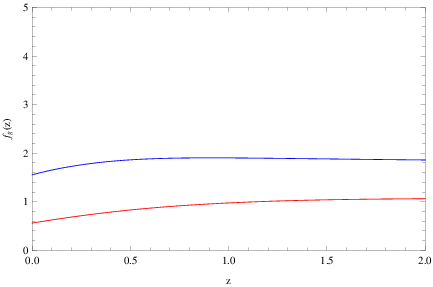
As it can be seen, the collisional matter generates matter perturbations (blue line) that differ significantly, in reference to non-collisional matter perturbations (red line). This behavior is to be contrasted to the behavior of the parameters that describe the cosmological evolution of the two different matter species, like for example the Hubble parameter, which case the evolution of collisional and non-collisional matter is almost identical (see left plot of Fig. 3). Before closing, we have to mention that there is another quantity that characterizes the growth of matter perturbations, related to the growth factor of matter perturbations $f_{g}(z)$ and also to the matter density parameter $\Omega_{m}(z)$, known as growth index $\gamma(z)$. The growth index is related to the aforementioned quantities as follows [45],

$$f_{g}(z)=\Omega_{m}(z)^{\gamma(z)}$$

(50)

The growth index cannot be observed directly but can be determined from the observational data of both $\Omega_{m}(z)$ and $f_{g}(z)$. For a detailed analysis of the growth index for the exponential model (9), see reference [45].

References

- [1] A.G. Riess et al. (High-z Supernova Search Team), Astronom. J. 116, 1009 (1998) [arXiv:astro-ph/9805201]
- [2] P.A.R. Ade et al. [arXiv:1302.5082]
- [3] P. A. R. Ade et al. [arXiv:1403.3985], (2014)
- [4] V. Mukhanov, Physical foundations of cosmology, Cambridge, UK: Univ. Pr. (2005) 421 p; D. S. Gorbunov, V. A. Rubakov, Introduction to the theory of the early universe: Cosmological perturbations and inflationary theory, Hackensack, USA, World Scientific (2011) 489 p
- [5] Yeuk-Kwan E. Cheung, J.D. Vergados, arXiv:1410.5710
- [6] V.K. Oikonomou, J.D. Vergados, Ch.C. Moustakidis, Nucl.Phys. B773 (2007) 19 [hep-ph/0612293]
- [7] S. Nojiri, S. D. Odintsov, Int.J.Geom.Meth.Mod.Phys. 11 (2014) 1460006 [arXiv:1306.4426]; Int. J. Geom. Meth. Mod.Phys. 4 (2007) 115 [hep-th/0601213]
- [8] S. Capozziello, V. Faraoni, Beyond Einstein Gravity, Springer, Berlin 2010
- [9] F. S. N. Lobo, Dark Energy-Current Advances and Ideas, 173-204 (2009) [arXiv:0807.1640]
- [10] S. Nojiri, S. D. Odintsov, Phys.Rept. 505 (2011) 59 [arXiv:1011.0544]
- [11] S. Capozziello, M. De Laurentis, Phys.Rept. 509 (2011) 167 [arXiv:1108.6266]
- [12] K. Bamba, S. Nojiri, S. D. Odintsov, JCAP 0810 (2008) 045 [arXiv:0807.2575]
- [13] S. Nojiri, S. D. Odintsov, Phys.Lett. B657 (2007) 238 [arXiv:0707.1941]
- [14] S. Capozziello, S. Nojiri, S.D. Odintsov, A. Troisi, Phys.Lett. B639 (2006) 135 [astro-ph/0604431]; S. Nojiri, S. D. Odintsov, Phys.Rev. D77 (2008) 026007 [arXiv:0710.1738]
- [15] S. Capozziello, V.F. Cardone, S. Carloni, A. Troisi, Int.J.Mod.Phys. D12 (2003) 1969 [astro-ph/0307018]
- [16] S. Nojiri, S. D. Odintsov, Phys.Rev. D74 (2006) 086005 [hep-th/0608008]; A. de la Cruz-Dombriz, A. Dobado, Phys.Rev. D74 (2006) 087501 [gr-qc/0607118]
- [17] W. Hu, I. Sawicki, Phys.Rev.D76 (2007) 064004 [arXiv:0705.1158]
- [18] S. M. Carroll, V. Duvvuri, M. Trodden, M. S. Turner, Phys.Rev. D70 (2004) 043528 [astro-ph/0306438]; S. Capozziello, Int.J.Mod.Phys.D11, 483 (2002) [gr-qc/0201033]
- [19] R. Myrzakulov, L. Sebastiani, S. Zerbini, Int.J.Mod.Phys. D22 (2013) 1330017 [arXiv:1302.4646]
- [20] O. Bertolami, R. Rosenfeld, Int.J.Mod.Phys. A23 (2008) 4817 [arXiv:0708.1784]
- [21] A. Capolupo, S. Capozziello, G. Vitiello, Int.J.Mod.Phys. A23 (2008) 4979 [arXiv:0705.0319]
- [22] P. K.S. Dunsby, E. Elizalde, R. Goswami, S. Odintsov, D. S. Gomez, Phys.Rev. D82 (2010) 023519 [arXiv:1005.2205]
- [23] G. Cognola, E. Elizalde, S. Nojiri, S.D. Odintsov, L. Sebastiani, S. Zerbini, Phys.Rev. D77 (2008) 046009 [arXiv:0712.4017 ]
- [24] K. Bamba, Chao-Qiang Geng, Chung-Chi Lee, JCAP 1008 (2010) 021 [arXiv:1005.4574]
- [25] S. Nojiri, S. D. Odintsov, D. Saez-Gomez, Phys.Lett. B681 (2009) 74 [arXiv:0908.1269]
- [26] S. Capozziello, V. F. Cardone, A. Troisi, Phys.Rev. D71 (2005) 043503 [astro-ph/0501426]
- [27] J. C.C. de Souza, Valerio Faraoni, Class.Quant.Grav. 24 (2007) 3637 [arXiv:0706.1223]; V. Faraoni, Phys.Rev. D74 (2006) 104017 [astro-ph/0610734];G. J. Olmo, Phys.Rev.Lett. 95 (2005) 261102 [gr-qc/0505101]; G. J. Olmo, Phys.Rev. D75 (2007) 023511 [gr-qc/0612047]
- [28] S. A. Appleby, R. A. Battye, A. A. Starobinsky, JCAP 1006 (2010) 005 [arXiv:0909.1737]
- [29] S. A. Appleby, R. A. Battye, Phys.Lett.B654 (2007) 7 [arXiv:0705.3199]; S. A. Appleby, R. A. Battye, JCAP 0805 (2008) 019 [arXiv:0803.1081]
- [30] A. Silvestri, M. Trodden, Rept. Prog. Phys. 72 (2009) 096901 [arXiv:0904.0024]
- [31] E. Elizalde, E.O. Pozdeeva, S.Yu. Vernov, Phys.Rev. D85 (2012) 044002 [arXiv:1110.5806]
- [32] V. Faraoni, Phys.Rev. D75 (2007) 067302 [gr-qc/0703044]
- [33] S. Nojiri, S. D. Odintsov, Phys.Rev. D68 (2003) 123512 [hep-th/0307288]
- [34] M. Sami, Curr. Sci. 97,887(2009) [arXiv:0904.3445]; Yi-Fu Cai, E. N. Saridakis, M. R. Setare, Jun-Qing Xia, Phys.Rept. 493 (2010) 1 [ arXiv:0909.2776]
- [35] T. Padmanabhan, Phys.Rept. 380 (2003) 235 [hep-th/0212290]; K. Bamba, S. Capozziello, S. Nojiri, S. D. Odintsov, Astrophys. Space Sci. 342, 155 (2012) [arXiv:1205.3421]
- [36] P.J.E. Peebles, Bharat Ratra, Rev.Mod.Phys. 75 (2003) 559 [astro-ph/0207347]; V. Sahni, AIP Conf.Proc. 782 (2005) 166, J.Phys.Conf.Ser. 31 (2006) 115; M. Li, Xiao-Dong Li, S. Wang, Yi Wang, Commun.Theor.Phys. 56 (2011) 525 [arXiv:1103.5870]; A. Joyce, B. Jain, J. Khoury, M. Trodden [arXiv:1407.0059]
- [37] V. Faraoni, Int.J.Mod.Phys. D11 (2002) 471 [astro-ph/0110067]; V.K. Onemli, R.P. Woodard, Class.Quant.Grav. 19 (2002) 4607 [gr-qc/0204065]
- [38] A. Gomez-Valent, J. Sola, S. Basilakos, arXiv:1409.7048; S. Basilakos, S. Nesseris, L. Perivolaropoulos, Phys.Rev. D87 (2013) 12, 123529; J. Khoury, A. Weltman, Phys. Rev. D69, 044026 (2004) [astro-ph/0309411 ]
- [39] Md. Wali Hossain, R. Myrzakulov, M. Sami, E. N. Saridakis, Phys.Rev. D89 (2014) 123513
- [40] Md. Wali Hossain, R. Myrzakulov, M. Sami, Emmanuel N. Saridakis, arXiv:1410.6100
- [41] V.K. Oikonomou, N. Karagiannakis, arXiv:1408.5353
- [42] K. Kleidis, N. K. Spyrou, Astron.Astrophys. 529 (2011) A26
- [43] V. Fock, The theory of space, time and gravitation, Pergamon Press, 1959, London UK
- [44] E. Elizalde, S.D. Odintsov, L. Sebastiani, S. Zerbini, Eur.Phys.J. C72 (2012) 1843 [arXiv:1108.6184]
- [45] K. Bamba, A. Lopez-Revelles, R. Myrzakulov, S.D. Odintsov, L. Sebastiani, Class.Quant.Grav. 30 (2013) 015008 [arXiv:1207.1009]
- [46] E. V. Linder, Phys.Rev. D80 (2009) 123528 [arXiv:0905.2962]
- [47] K. Bamba, A. Lopez-Revelles, R. Myrzakulov, S.D. Odintsov, L. Sebastiani, TSPU Bulletin 13 (2012) 128, 22-27 [arXiv:1301.3049]
- [48] V.K. Oikonomou, Gen.Rel.Grav. 45 (2013) 2467 [arXiv:1304.4089 ]
- [49] J. Matsumoto, Phys.Rev.D83 (2011) 124040 [arXiv:1105.1419]
- [50] S. Capozziello, M. De Laurentis, O. Luongo, arXiv:1411.2822
- [51] A. de la Cruz-Dombriz, A. Dobado, A. L. Maroto, Phys.Rev.D77 (2008) 123515 [arXiv:0802.2999]