Buffer occupancy asymptotics in rate proportional sharing networks with heterogeneous long-tailed inputs

Modern networks carry many different types of traffic streams with widely differing characteristics. The statistical variations that are of primary interest are those which are short lived and those that are long flows. The reason is that these two types of flows have very different impacts in terms of engineering the network in terms of router speeds and buffering requirements. The key issue is that long duration flows must be handled carefully and their statistical characteristics usually are the dominant ones in terms of network queueing performance. On the time-scale of long flows, short flows can be viewed as averaged out and while they can take up bandwidth it is predictable and thus the primary situation of interest is one in which long-lived flows are present. A detailed statistical analysis of such sessions suggests that they are well modelled by ON-OFF type of processes where the ON periods, of random duration, have a tail distribution which decays according to a long-tailed distribution. Different definitions are used in the literature for long and heavy tails. Here we assume that a r.v. $X$ is long-tailed if $\hbox{${\rm I\hskip-2.0ptP}$}\{X>x\}\sim const.\ x^{-\beta}$ with $\beta>0$. If $\beta\in(0,2]$, then $X$ has infinite variance and is said to heavy-tailed. These distributions are said to be sub-exponential. When many independent such sessions arrive randomly, the aggregated input process is long-range dependent.

The performance of networks and their ability to offer Quality of Service (QoS) depend on accurately capturing the parametric dependence of the QoS measures such as the delay or loss distributions. While calculating these distributions exactly is intractable, the asymptotics of the tail distribution are much more manageable.

Numerous studies have shown that the presence of long and heavy-tailed traffic forces us to change the way the buffer dimensioning is done in that much more buffering is necessary to achieve similar buffer overflow characteristics than with conventional or short-range dependent traffic. Indeed, the way buffer overflows occur can be very different. This is essentially due to the way that large excursions of the buffer workload take place. For conventional traffic models, the tail of the stationary workload distribution is exponential while for long-range dependent traffic, it has an asymptotic long-tail or sub-exponential decay.

There are many results available for buffer asymptotics of a single node or server with long-tailed and sub-exponential inputs. These have been obtained under different hypotheses. These hypotheses relate to conditions on the session length distribution decay rates, session transmission rates and session arrival models. All results deal with stationary queues where the average rate is less than capacity. The vast majority of results are for FIFO systems where the source transmission rates are identical, which is referred as the homogeneous case. These can be found, for example, in [11, 19, 22, 17, 26, 27]. An excellent survey for the homogeneous case can be found in [8]. It has however been shown in [21] that assuming the same transmission rates can lead to erroneous conclusions on the asymptotic behavior of the tail distribution of the buffer length when the inputs have long-tailed session lengths. This was obtained for the so-called $M/G/\infty$ model where sessions arrive according to a Poisson process, transmit at different rates and have differing long-tailed random session holding times. Similar results and conclusions have also been obtained for a fixed number of ON-OFF sources in [7]. Since these early papers there have been a number of works on studying the effects of sub-exponential distributions and how they arise in the context of network traffic, see [19] and references therein.

The extension of above results to a general network is quite difficult since the traffic loses its simple parametric structure after passing through its entrance node. Networks with exponentially distributed service times were considered in [3] and [14]. In [23], the author studied the large deviations problem for feedforward networks in heavy traffic. The papers were basically concerned with the computation of the rate functions associated with the tail distributions of the buffer occupancy. This is a difficult variational problem. In general, when the input and output rate functions in queues have the so-called “linear geodesics” an end-to-end analysis is feasible by an iterative procedure. In [15, 24], it was shown that in queues with many inputs the linear geodesic property does not hold and thus calculating the rate functions of the outputs is difficult.

There are very few results available for networks with long-tailed service times. In [6], the authors consider the (max, plus) setting and derive asymptotics of the distributions of total response times for networks which include tandem queues. In [18], a feedforward network is analyzed when a node with sub-exponential service time has upstream nodes with lighter-tailed service times. In spite of these early successes the network case with general long-tailed have been analyzed only for very special cases such as feed-forward, or tandem networks [20]. Most network models assume service times are i.i.d at nodes with sub-exponential distributions. In reality, flows do not change their sizes and thus the analysis must take into account the fact that within the networks the service times are no more independent. A recent issue [1] devoted to network asymptotics does not address the issue of network buffer distributions. Thus, except for special network models that do not correspond to flow type session traffic there are no explicit results available that characterize the stationary buffer distributions.

In this paper we consider the model where sessions arrive independently as Poisson processes and transmit at a fixed rate during their session duration. At a given node when the server capacity is exceeded, the capacity is shared in proportion to the rates of the flows else the source passes through unchanged. This is often referred to as rate proportional sharing and can be viewed as a discriminatory processor sharing discipline (DPS) [2] that approximates a weighted based round-robin service where the weights correspond to the rates of the flows entering the router. The rate multiplied by the number of flows denotes the aggregated required bandwidth of the flows. The session or flow durations are assumed to be long-tailed, having an asymptotic power law or generalized Pareto decay. The sessions are assumed to be heterogeneous so that they have different session duration distributions and different transmission rates. This gives rise to an heterogenous $M/G/\infty$ type of model for the inputs. It is assumed that the types of sessions are defined by the routes that they take through the network and it is assumed that paths are loop-free. Although the path for a single end-to-end route is loop free, the interaction between the flows in the network creates dependence between flows within the network, i.e., the input characterization is changed. In particular the probabilistic characterization of the duration and rates changes due to the sharing of the processors. We obtain the $O$-asymptotics (i.e. we identify the asymptotic power law decay) for the buffer occupancies at each node. In particular it shows that the characterization of the decay rate as the solution an optimal knapsack problem for a single server carries through to the network case with changes in the rates. The utility of this result is that we can identify the sources that are the most problematic and also obtain rough estimates for the loss and delay distributions. These results extend to networks with rate proportional sharing the results that were obtained in  [21] however it is now more complicated due to the fact that output processes are difficult to characterize in non-Markovian settings. In the single node case, exact asymptotics of buffer occupancy and loss obtained in [21] showed that these asymptotics are not only governed by the tail distribution of sources but also depend on their transmission rates that could be obtained from a knapsack problem. This result was also obtained in [28] using the idea of equilibrium service times pioneered by Pakes [25] for tails sub-exponential inputs to a queue.

In this paper we show that a similar characterization also holds in a general loop-free network with rate proportional sharing. However computing the exponents of the buffer tail distributions need us to first solve a fixed point problem. This is because the interaction of traffic inside the network causes transmission rates and average load rates to be modified during long buffer exceedance times. Furthermore, since we do not assume that the network is feedforward, it results in a fixed point equation for computing the “modified” rates. It is difficult to improve these results (e.g. obtain exact asymptotics) since the Poisson arrival structure and independence of sessions are lost for the traffic inside the network.

The organization of this paper is as follows: In Section 2, we formulate the model and present the preliminaries. Section 3 contains the main result with the proofs. An example of a two node network is considered in Section 4. In Section 5, we give a discussion of results and concluding remarks.

We consider a discrete-time fluid DPS model where traffic arrivals and services take place in slots indexed by $t\in\hbox{\rm Z\hskip-4.0ptZ}$ with the convention that arrivals take place at the beginning of a slot and services are completed at the end of the slot. This can be seen as corresponding to a situation in the continuous time where the arriving traffic coming in $(i,i+1]$ are all served at time $i+1$. We refer to $t$ as the time instant in the discrete-time model. There is a finite set $\mathcal{N}$ of traffic types (classes) with $N=card(\mathcal{N})$ which are differentiated according to their transmission rates and their session lengths and different classes are assumed to be mutually independent. Session requests for type $n\in\mathcal{N}$ arrive randomly according to a Poisson process with rate $\lambda_{n}$. Let $\theta^{n}_{t}$ be the number of sessions of class $n$ arriving at time $t$. We assume that $\theta^{n}_{t}$ are i.i.d. for fixed $n$ and

A session of class $n$ then transmits at the rate $r_{n}$ (bits/slot) for a duration $\tau_{n}$ (slots) which is assumed to have a long-tailed distribution. Let $\tau^{n}_{t,j}$ denote the session length of the $j$’th session of class $n$ arriving at time $t.$ The r.v.’s $\tau^{n}_{t,j}$ are assumed to be i.i.d. for fixed $n$ and satisfy

where $\alpha_{n},\beta_{n}>0$ and $A(x)\sim B(x)$ means that $\lim_{x\rightarrow\infty}\frac{A(x)}{B(x)}=1$. Also $A(x)\preceq(\succeq)B(x)$ means $\limsup_{x\rightarrow\infty}\frac{A(x)}{B(x)}\leq 1(\liminf_{x\rightarrow\infty}\frac{A(x)}{B(x)}\geq 1)$, i.e., the inequalities are in an asymptotic sense. This model is a generalization of the $M/G/\infty$ model proposed by Cox [9], which we refer to as the $(M/G/\infty)^{N}$ model and is depicted in Fig. 1.

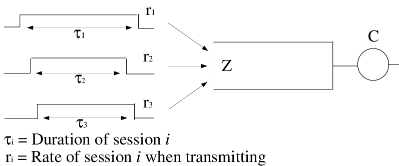
The network is composed of $M$ nodes (see Fig. 2 below). It is assumed that the packets from the sessions are admitted into an infinite buffer and the buffer is served at a rate of $C_{m}$ per unit time at node $m=1,\ldots,M$. The capacity is shared in proportion to the number of sessions and their rates. Type $n\in\mathcal{N}$ traffic has a fixed route without any loops and its path is represented by the vector ${\pi}^{n}=\left[\pi^{n}_{1},\ldots,\pi^{n}_{l_{n}}\right]$ where $\pi_{i}^{n}\in\{1,\ldots,M\}$. Hence, type $n$ traffic traverses the nodes by entering the network at node $\pi^{n}_{1}$ and leaving after node $\pi^{n}_{l_{n}}$ and $\pi_{i}^{n}\neq\pi_{j}^{n}$ for $i\neq j$. We define the set of traffic types which pass through node $m$ by ${\mathcal{N}_{m}}\doteq\{n\in\mathcal{N}:\ \pi_{i}^{n}=m,\ 1\leq i\leq l_{n}\}$.

Let $X^{n}_{t}$ be the input traffic process of class $n$ entering the network. Then,

and average (mean) load of class $n$ is

Let $W^{m,n}_{t}$ denote the workload due to a flow of type $n$ at server $m$ and

denote the total work due to all flows at server $m$.

Let

Under this hypothesis, the queues in the network are stable since the network is loop-free for all classes of flows. condition, by Loynes’ theorem [5], there exists a stationary version of $W^{m}$.

Consider the following splitting of the input process $X^{n}_{t}$ into two processes $X^{n,L}_{t}$ and $X^{n,H}_{t}$ as follows: The process $X^{n,L}_{t}$ is formed by active sessions which have session lengths at most $\varepsilon z$ (will be referred as “short” sessions in the context) with $\varepsilon>0$ and given by

In the sequel, $z$ will be taken as the large buffer occupancy level and $\varepsilon>0$ will be chosen to be a small enough number. The process $X^{n,H}_{t}$ is composed of sessions with lengths greater than $\varepsilon z$ (will be referred as “long” sessions in the sequel) and given by

As it can be seen from the definition, the processes $X^{n,L}_{t},X^{n,H}_{t}$ are mutually independent and $X^{n}_{t}=X^{n,L}_{t}+X^{n,H}_{t}$. The superscript ‘$H$’ indicates that the process is strictly “heavy” (or “long”) and the superscript ‘$L$’ indicates that the process is strictly “light” (or “short”). We will refer to $X^{n,L}$ and $X^{n,H}$ as short and long processes in this context. As $z\rightarrow\infty,$ we have ${\hbox{${\rm I\hskip-2.0ptE}$}}X^{n,L}_{t}\rightarrow{\hbox{${\rm I\hskip-2.0ptE}$}}X^{n}_{t}$ and ${\hbox{${\rm I\hskip-2.0ptE}$}}X_{t}^{n,H}\rightarrow 0$. Despite the fact that ${\hbox{${\rm I\hskip-2.0ptE}$}}X^{n,H}_{t}\rightarrow 0$ as $z\rightarrow\infty$, the process $X^{n,H}_{t}$ will contribute significantly to the large buffer occupancy probability.

Later, we will choose $\varepsilon$ small enough so that the short sessions can be replaced with constant inputs without any effect on the buffer length O-asymptotics.

We define $X^{n}_{k,t}$ ($Y^{n}_{k,t}$) to be the class $n$ input (output) traffic at node $k$ and time $t$. For any process $Z$ with value $Z_{t}$ at time $t$, the cumulative process in the time interval $(t_{1},t_{2}]$ will be denoted by $Z(t_{1},t_{2})$, i.e., $Z(t_{1},t_{2})=\sum_{i=t_{1}+1}^{t_{2}}Z_{t}.$

We also need the following definitions to state the main result. Let $J\in\hbox{\rm Z\hskip-4.0ptZ}_{+}^{N}$ where $\hbox{\rm Z\hskip-4.0ptZ}_{+}=\{0,1,2,\ldots\}$. $J$ will correspond to the combination of long (longer than $\varepsilon z$) sessions; i.e. there are $J_{n}$ long sessions of class $n$. If the transmission rates of active long sessions at a time exceed the difference of total output capacity and average load at a node, a scaling effect would occur. This happens because the service capacity is shared among all these active sessions according to rate proportional scheduling and at times when there is not enough output capacity at a node to serve all the traffic without buffering, the output process of this node will behave as a scaled version of its input process. In particular, the mean load of short sessions (which goes to the average workload as $z\rightarrow\infty$) and the transmission rates of long sessions would change at the output. In order to quantify this, we first define $p^{n}(m)=m^{\prime}$ for $n\in\mathcal{N}_{m}$ if $\pi^{n}_{i}=m$ and $\pi^{n}_{i-1}=m^{\prime}$; i.e. $p^{n}(m)$ is the upstream node of node $m$ for class $n$. Take $p^{n}(m)=0$ if $m=\pi^{n}_{1}$. We define the transmission rate and mean of class $n$ traffic entering node $m$ as follows:

and

where

$S^{J}_{m}$ is just the fraction of the capacity available to each flow at the node $m$ and so $r_{n}S^{J}_{m}$ would be the rate allocated to flow $n$ at node $m$ with configuration of $J$ long flows. Note that the output traffic is no longer $M/G/\infty$ .

The function $S^{J}_{m}$ measures the scaling of sources for the output transmission at node $m$ for a combination of $J$ active long sessions. Note that $0<S^{J}_{m}<1$ when the input rates of the long sessions exceed the difference between the output capacity and the total average loads at node $m$ and $S^{J}_{m}=1$ if this does not happen.

Proof. See Appendix A.

We now define the following for future usage:

The results below, taken from [21] (Lemma 3.3 and Lemma 3.4 therein), provide bounds for the deviations of a short process from its average rate.

Our goal is to obtain the $O$-asymptotics for the probability that the buffer content at node $m$ exceeds a large value $z$. We will use $f(z)=O(g(z))$ to mean $0<\liminf_{z\rightarrow\infty}f(z)/g(z)\leq\limsup_{z\rightarrow\infty}f(z)/g(z)<\infty$ and $f(z)=o(g(z))$ to mean $0<\lim_{z\rightarrow\infty}f(z)/g(z)=0$. It will be shown that the buffer of node $m$ will reach a large value $z$ if there are enough number of long sessions which contribute to this. During this time, the short sessions show average behavior, i.e., produce traffic around their mean load level. Thus, the short processes can be replaced with constant (equal to the mean load) processes in the asymptotic regime without causing a significant change at large occupancy levels of buffers.

We first review the single node result ($M=1$) from [21] (Theorem 2.1 therein) where exact buffer asymptotics were obtained. A form of their result, sufficient for our purposes in this paper, is

It was shown in [21] also that the most likely large buffer occupancy is generated by a busy period when exactly $J^{1}_{0}$ long sessions are active during this busy period. If there is only a single type of flow ($card(\mathcal{N})=1$), then $J^{1}_{0}=\lceil(C_{1}-\rho_{1})/r_{1}\rceil$. Hence the buffer length decay rate $\kappa_{J^{1}_{0}}$ depends not only on the decay rates $\beta_{n}$’s but also on the transmission rates $r_{n}$’s unless $r_{1}>C_{1}-\rho_{1}$ in which case $J^{1}_{0}=1$.

The basic idea of the proof is the following (that is valid at a single buffer with independent short and long processes ):

Let $\{Y_{t}\}$ denote the input process to a buffer that operates at rate $C_{m}$ and $Y^{L}$ and $Y^{H}$ refer to the short and long inputs defined in (2) and (3) and thus:

with $\hbox{${\rm I\hskip-2.0ptE}$}[Y_{t}]=\sum_{n\in\mathcal{N}_{m}}\rho_{n}<C_{m}$. In the following sketch of the ideas for simplicity we set $\sum_{n\in\mathcal{N}_{m}}\rho_{n}=\rho$.

Having defined this decomposition of $\{Y_{t}\}$ the basic idea of the proof is as follows.

References

- [1] Queueing systems (questa): Special issue on stochastic networks: Tail asymptotics for stationary distributions and related topics. volume Volume 74, Issue 2-3, pages 105–368. 2013.
- [2] E. Altman, K. Avrachenkov, and U. Ayesta. A survey on discriminatory processor sharing. Queueing Systems, 53(1-2):53–63, 2006.
- [3] V. Anantharam. Networks of queues with long-range dependent traffic streams. In Stochastic networks, volume 117 of Lecture Notes in Statist., pages 237–256. Springer, New York, 1996.
- [4] S. Asmussen. Applied probability and queues, volume 51 of Applications of Mathematics (New York). Springer-Verlag, New York, second edition, 2003.
- [5] F. Baccelli and P. Brémaud. Elements of Queueing Theory, Series in Applications of Mathematics 26. Springer-Verlag, N.Y., 1994.
- [6] F. Baccelli, S. Schlegel, and V. Schmidt. Asymptotics of stochastic networks with subexponential service times. Queueing Systems, 33, No. 1-3:205–232, 1999.
- [7] S. Borst, O. Boxma, and P. Jelenkovic. Generalized processor sharing with long-tailed traffic sources. In P. Key and D. Smith, editors, Teletraffic Engineering in a Competitive World, pages 345–354. Elsevier, 1999.
- [8] O. J. Boxma and V. Dumas. Fluid queues with long-tailed activity period distributions. Computer Communications, 21:1509–1529, 1998.
- [9] D. R. Cox. Long-range dependence: A review. In H. A. David and H. T. David, editors, Statistics: An appraisal. Iowa State University Press, Ames, Iowa, 1984.
- [10] K. Deimling. Nonlinear functional analysis. Springer-Verlag, Berlin, 1985.
- [11] N. G. Duffield and N. O’Connell. Large deviations and overflow probabilities for the general single-server queue, with applications. Math. Proc. Cambridge Philos. Soc., 118(2):363–374, 1995.
- [12] W. Feller. An introduction to probability theory and its applications, Vol. II. Wiley, N.Y., 1966.
- [13] S. Foss, D. , Korshunov, and S. Zachary. An introduction to heavy-tailed and subexponential distributions. Springer Series in Operations Research and Financial Engineering. Springer, New York, 2011.
- [14] A. Ganesh and V. Anantharam. Stationary tail probabilities in exponential server tandems with renewal arrivals. Queueing Systems, 22:203–248, 1996.
- [15] A. J. Ganesh and N. O’Connell. The linear geodesic property is not generally preserved by a FIFO queue. Annals of Applied Probability, 8(1):98–111, 1998.
- [16] F. R. Gantmacher. The theory of matrices. Vol. 1. AMS Chelsea Publishing, Providence, RI, 1998. Translated from the Russian by K. A. Hirsch, Reprint of the 1959 translation.
- [17] D. Heath, S. Resnick, and G. Samorodnitsky. Heavy tails and long-range dependence in on/off processes and associated fluid models. Mathematics of Operations Research, 23:145–165, 1998.
- [18] T. Huang and K. Sigman. teady-state asymptotics for tandem, split-match and other feedforward queues with heavy-tailed service. Queueing Systems, 33:233–259., 1999.
- [19] P. R. Jelenkovic and A. A. Lazar. Asymptotic results for multiplexing subexponential on-off sources. Advances in Applied Probability, 31:394–421, 1999.
- [20] J-K. Kim. Tail asymptotics of queueing networks with subexponential service times. PhD thesis, Georgia Institute of Technology, 2009.
- [21] N. Likhanov and R. R. Mazumdar. Loss asymptotics in large buffers fed by heterogeneous long-tailed sources. Adv. in Appl. Probab., 32(4):1168–1189, 2000.
- [22] Z. Liu, P. Nain, D. Towsley, and Z-L. Zhang. Asymptotic behavior of a multiplexer fed by long-range dependent process. Journal of Applied Probability, 36(1):105–118, 1999.
- [23] K. Majewski. Large Deviations of Feedforward Queueing Networks. PhD thesis, Ludwig-Maximilian-Universitat, Munchen, 1996.
- [24] N. O’Connell. Large deviations for departures from a shared buffer. J. Appl. Probab., 34(3):753–766, 1997.
- [25] A. G. Pakes. On the tails of waiting-time distributions. J. Appl. Probab., 12:555–564, 1975.
- [26] M. Parulekar and A. M. Makowski. Tail probabilities for input processes. Queueing Systems, 27:271–296, 1997.
- [27] T. Rolski, S. Schlegel, and V. Schmidt. Asymptotics of Palm-stationary buffer content distributions. Advances in Applied Probability, 31:235–253, 1999.
- [28] B. Zwart, S. Borst, and M. Mandjes. Exact asymptotics for uid queues fed by multiple heavy-tailed on-off sources. Annals of Applied Probability, Vol. 14:903–957, 2004.
Appendix A Proof of Lemma 2.1
We will show that and form a unique fixed point of a function for a given set of values of . Let us now describe this function: Let , and define
Here vector corresponds to the transmission rates and average loads of the flows at all nodes. Now for , define the function such that