Acknowledgement

PhD Thesis

Query-driven Data Completeness Management

Author:

Simon Razniewski

Supervisor:
Prof. Werner Nutt

Thesis in part reviewed by:

- Prof. Leopoldo Bertossi, Carleton University, Canada

- Prof. Jan van den Bussche, Universiteit Hasselt, Belgium

- Prof. Floris Geerts, University of Antwerp, Belgium

- Prof. Francesco Ricci, Free University of Bozen-Bolzano, Italy

- Prof. Fabian M. Suchanek, Télécom ParisTech University, France

October 2014

There are two kinds of methodologies:

1. Those that cannot be used to reason about incomplete information

Acknowledgement

First of all I would like to thank my advisor for his advice, guidance and patience. I would also like to thank to my close colleagues and my coauthors, in particular Ognjen Savkovic, Marco Montali, Fariz Darari and Giuseppe Pirró. I would like to thank my collaborators, in particular Divesh Srivastava, Flip Korn, Marios Hadjieleftheriou and Alin Deutsch. I am thankful for the good surrounding and support from my colleagues in the KRDB group and in the Faculty of Computer Science. Thanks to my friends. Thanks to my family. Thanks to Mita.

Abstract

Knowledge about data completeness is essentially in data-supported decision making. In this thesis we present a framework for metadata-based assessment of database completeness. We discuss how to express information about data completeness and how to use such information to draw conclusions about the completeness of query answers. In particular, we introduce formalisms for stating completeness for parts of relational databases. We then present techniques for drawing inferences between such statements and statements about the completeness of query answers, and show how the techniques can be extended to databases that contain null values. We show that the framework for relational databases can be transferred to RDF data, and that a similar framework can also be applied to spatial data. We also discuss how completeness information can be verified over processes, and introduce a data-aware process model that allows this verification.

Publication Overview

Conference Publications

•

Simon Razniewski and Werner Nutt. Adding completeness information to query answers over spatial databases. International Conference on Advances in Geographic Information Systems (SIGSPATIAL), 2014.
•

Simon Razniewski, Marco Montali, and Werner Nutt. Verification of query completeness over processes. International Conference on Business Process Management (BPM), pages 155–170, 2013. Acceptance rate 14,4%.
•

Fariz Darari, Werner Nutt, Giuseppe Pirrò, and Simon Razniewski. Completeness statements about RDF data sources and their use for query answering. International Semantic Web Conference (ISWC), pages 66–83, 2013. Acceptance rate 21,5%.
•

Simon Razniewski and Werner Nutt. Assessing the completeness of geographical data (short paper). British National Conference on Databases (BNCOD), 2013. Acceptance rate 47,6%.
•

Werner Nutt and Simon Razniewski. Completeness of queries over SQL databases. Conference on Information and Knowledge Management (CIKM), pages 902–911, 2012. Acceptance rate 13,4%.
•

Simon Razniewski and Werner Nutt. Completeness of queries over incomplete databases. International Conference on Very Large Databases (VLDB), 2011. Acceptance rate 18,1%.

Other Publications

•

Simon Razniewski, Marco Montali, and Werner Nutt. Verification of query completeness over processes [extended version]. CoRR, abs/1306.1689, 2013.
•

Werner Nutt, Simon Razniewski, and Gil Vegliach. Incomplete databases: Missing records and missing values. DQDI workshop at DASFAA, 2012.
•

Simon Razniewski and Werner Nutt. Checking query completeness over incomplete data. Workshop on Logic and Databases (LID) at ICDT/EDBT, 2011.

^†^†margin: 1 Introduction

Decision processes in businesses and organizations are becoming more and more data-driven. To draw decisions based on data, it is crucial to know about the reliability of the data, in order to correctly assess the trustworthiness of conclusions. A core aspect of this assessment is completeness: If data is incomplete, one may wrongly believe that certain facts do not hold, or wrongly believe that a derived characteristics are valid, while in fact the present data does not represent the complete data set, which may have different characteristics. With the advent of in-memory database systems that merge the traditionally separated transaction processing (OLTP) and decision support (OLAP), data quality and data completeness assessment are also topics that require more timely treatment than in the traditional setting, where transaction data and data warehouses are separate modules.

This work is motivated by a collaboration with the school department of the Province of Bolzano, which faces data completeness problems when monitoring the status of the school system. The administration runs a central database into which all schools should regularly submit core data about pupil enrollments, teacher employment, budgets and similar. However, as there are numerous schools in the province and as there are various paths to submit data (database clients, Excel-sheets, phone calls, …), data for some schools is usually late or data about specific topics is missing. For instance, when assigning teachers to schools for the next school year, it is often the case that the data about the upcoming enrollments is not yet complete for some schools. In practice, decisions are then based on estimates, for instance using figures from the previous year. Completeness information would greatly help the decision makers to know which figures are reliable, and which need further checks and/or estimates.

In this thesis, we discuss a framework for metadata-based data completeness assessment. In particular, we present:

(i)

an investigation into reasoning about the completeness of query answers including decision procedures and analyses of the complexities of the problems,
(ii)

an extension of completeness reasoning to geographical databases and to RDF data,
(iii)

a formalization of data-aware processes and methods to extract completeness statements from such process descriptions.

The rest of this chapter is structured as follows. In Section 1 we give a general introduction to the area of Data Quality and to the problem of data completeness. In Section 2 we illustrate the problem of data completeness management with the example of school data management. Section 3 summarizes the contributions in this thesis and in Section 4 we explain the outline of this thesis.

1 Data Quality and Data Completeness

Quality is a vague term, and this also transfers to data quality. A general definition that most people concerned with data quality could agree with is that data are of high quality “if they are fit for their intended uses in operations, decision making and planning” [39].

Data quality has been a problem since long. With the emergence of electronic databases in the 1960s, creation and storage of larger volumes of data has become easier, leading also to more potential data quality problems. Since the very beginning, data quality has been an issue in relational databases, e.g., keys were introduced in order to avoid duplicates [18]. As an independent research area, data quality has gained prominence in the 1990s. Three areas of data quality have received particular attention:

(i)

The first area is duplicate detection, which is also referred to as entity resolution, and which is one of the most important operations within data cleansing [36, 88]. It seems that this is the most common practical problem that nearly any business that manages customer relations will run into.
(ii)

The second area are guidelines and methodologies for assessing and improving data quality, with a prominent one being the TDQM methodology [86, 53].
(iii)

The third area are approaches for dealing with data quality in data integration settings, which are particularly concerned with integration techniques [54] or methods for identifying data sources that best satisfy certain information needs [61].

Since the very beginning, relational databases have been designed so that they are able to store incomplete data [19]. The theoretical foundations for representing and querying incomplete information were laid by Imielinski and Lipski [47] who captured earlier work on Codd-, c- and v-tables with their conditional tables and introduced the notion of representation system. Later work on incomplete information has focused on the concepts of certain and possible answers, which formalize the facts that certainly hold and that possibly hold over incomplete data [31, 54, 2]. Still, most work on incompleteness focuses on querying incomplete data, not on the assessment of the completeness. A possible reason is that unlike consistency, completeness can hardly be checked by looking at the data itself. If one does not have another complete data source to compare with, then except for missing values, incompleteness is not visible, as one cannot see what is not present. As well, incompleteness can only be fixed if one has a more complete data source at hand that can be used, which is usually not the case as then one could directly use that more complete data source.

In turn, if metadata about completeness is present, an assessment of the completeness of a data source is possible. As queries are the common way to use data, we investigate in particular how such metadata can be used to annotate query answers with completeness information.

In difference to data cleansing, we do not aim to improve data quality, but instead aim to give a usage-specific information about data quality. In difference to the guidelines and methodologies, we do not give hints on how to improve data quality, but instead focus on the algorithmic question of how to logically reason about completeness information. In contrast to the approaches in the area of data integration, we do not investigate source selection optimization or query semantics over incomplete data.

There has been previous work on metadata-based completeness assessment of relational databases. A first approach is by Motro [59], who used information about complete query answers to assess the completeness of other query answers. Later on, Halevy, introduced the idea of using statements about the completeness of parts of a database to assess the completeness of query answers [56]. In both works, the problem of deciding whether a query answer is complete based on completeness metadata could only be answered in a few trivial cases.

In the next section, we see a motivating story for this research.

2 Motivation

Consider the school district administrator Alice. Her job in the administration is to monitor the impacts of new teaching methodologies, special integration programs and socioeconomic situations on learning outcomes of students.

As last year a new, more interactive teaching methodology was introduced for Math courses, Alice is interested to see whether that shows any impact on the performance on the students. So, two weeks after the end of the school year, she uses her cockpit software to find out how many pupils have the grade A in math.

The results show that at high schools, the number changed insignificantly by +0.3%, while at middle schools the tool reports a drop of 37% compared to the last year.

Alice is shocked about this figure, and quickly calls her assistant Frank to investigate this drop.

Frank calls several middle schools and questions them about the performance of their students in Math. All schools that he calls say that the Math results of their students are as usual.

Confused from hearing that the schools report no problems, Frank suspects that something must be wrong with the cockpit software. He therefore sends an email to Tom, the database administrator.

Tom’s answer is immediate:

Dude, forget those figures, we don’t have the data yet.

-tom

As Frank tells this to Alice, she is relieved to hear that the new teaching methodology is not likely to have wrecked the Math performance. Nevertheless she is upset to not know which data in the cockpit she can actually believe in and which not. Maybe the brilliant results of last year’s sport campaign (-80% overweight students) were actually also due to missing data?

Alice orders the IT department to find a solution for telling her which numbers in the cockpit are reliable and which not.

A week later, at a focus group meeting organized by Tom, all participants quickly agree that it is no problem to know which data in the database is complete. They just have to keep track of the batches of data that the schools submit. However, how can they turn this information into something that Alice can interpret? They decide that they need some kind of reasoner, which attaches to each number in Alice’s cockpit a green/red flag telling her whether the number is reliable. Developing this reasoner becomes Tom’s summer project (Chapter 3).

At the end of the summer break, the reasoner seems successfully implemented. However just during the presentation to Alice, the reasoner crashes with the following error message:

java.lang.NullpointerException("Grade is null")

As it turns out, a null value for a grade caused the reasoner to crash. Thus back to coding, Tom gets stuck when thinking of whether to treat such null values as incomplete attributes or as attributes that have no value. As it turns out after consultations with the administration, both cases happen: Some courses are just generally ungraded, while in other cases the grade may not yet be decided. As the reasoner has to know which case applies, Tom finds himself changing the database schema to allow a disambiguation of the meaning of null values (Chapter 4).

In his free time, Tom is also a member of the OpenStreetMap project for creating a free open map of the world. During some pub meeting with other members of OpenStreetMap he mentions his work on database completeness. The others get curious. Don’t they have similar problems when trying to track completeness information in OpenStreetMap? Tom therefore invents reasoning methods for geographical data (Chapter 5).

In the meantime, Alice is very satisfied with the new green and red flags in her cockpit software. She has a chat about this with some colleagues of the provincial administration, which are involved in the ongoing data publishing projects as part of the Open Government initiative in the province. They consult again Tom, who adapts his reasoner to deal also with the RDF data format that is used for data publishing, and the SPARQL query language (Chapter 6).

In their efforts to standardize processes at schools, the administration introduces a workflow engine. It now becomes a question how information about of the states of the workflows of the different schools can be utilized to assess query completeness. Thus, they investigate how business process state information can be used to automatically extract information about completeness (Chapter 7).

3 Contribution

The contributions of this thesis are threefold:

First, we introduce the reasoning problems of TC-TC entailment, TC-QC entailment and QC-QC entailment and show that most variants of these problems can be reduced to the well-studied problem of query containment, thus enabling implementations that can make use of a broad set of existing solutions.

Second, we show that completeness reasoning can also be done over RDF data or over geographical data, and that the additional challenges in this settings are manageable.

Third, we show that in settings where data is generated by formalized and accessible processes, instead of just assuming that given completeness statements are correct, one instead can verify the completeness of query answers by looking at the status of the processes.

4 Structure

This thesis is structured as follows:

In Chapter 2, we introduce relational databases, queries over such databases and formalisms for expressing completeness. In Chapter 3, we introduce the core reasoning problems and discuss their complexity. In Chapter 4, we extend the core framework by allowing null values in databases. In Chapter 5, we discuss completeness reasoning over geographical databases. In Chapter 6, we discuss completeness reasoning over RDF data. In Chapter 7, we show how completeness statements can be verified over data-centric business processes. In Chapter 8, we discuss implications of the presented results, possible limitation, and future directions.

^†^†margin: 2 Preliminaries

In this chapter we discuss concepts and notation that are essential for the subsequent content. In Section 5, we introduce the running example used throughout this thesis. We introduce relational databases and their logical formalization in Section 6. In Section 7, we formalize queries over relational databases, focusing on the positive fragment of SQL. In Section 8 we introduce the model for incompleteness of databases, and in Sections 9 and 10 two important kinds of completeness statements about incomplete databases, namely table completeness and query completeness statements. In Section 11, we recall the problem of query containment, onto which many later problems will be reduced, and review its complexity.

The concepts presented in this chapter were already known in the literature, though our presentation may be different. On the complexity of query containment, we present three new hardness results.

5 Running Example

For the examples throughout this thesis we consider a database about schools. We assume that this database consists of the following tables:

•

$\mathit{student}(\mathit{name},\mathit{class},\mathit{school})$
•

$\mathit{person}(\mathit{name},\mathit{gender})$
•

$\mathit{livesIn}(\mathit{name},\mathit{town})$
•

$\mathit{class}(\mathit{school},\mathit{code},\mathit{formTeacher},\mathit{profile})$
•

$\mathit{result}(\mathit{name},\mathit{subject},\mathit{grade})$
•

$\mathit{request}(\mathit{name},\mathit{school})$

As this is just a toy example, we assume that persons are uniquely identified by their name (in practice one would assign unique IDs or use nearly unique combinations such as birth data and birth place). The $\mathit{student}$ table stores for each student the class and the school that he/she is attending. The $\mathit{person}$ table stores for persons such as students and teachers their gender. The $\mathit{livesIn}$ table stores for persons the town they are living in. The $\mathit{result}$ table stores for students the results they have obtained in different subjects. The $\mathit{request}$ table stores enrollment requests of current or upcoming students at schools.

6 Relational Databases

Relational databases are a very widely used technology for storing and managing structured data. The formal background of relational databases is the relational data model. A database schema consists of a set of relations, where each relation consists of a relation name and a set of attributes. A relation usually represents either an entity type or a logical relation between entity types.

To model relational databases, we assume a set of relation symbols $\Sigma$ , each with a fixed arity. We call $\Sigma$ the signature or the database schema. We also assume a dense ordered domain of constants $\mathit{dom}$ , that is, a domain like the rational numbers or like the set of possible strings over some alphabet.

Definition 2.1.

Given a fixed database schema $\Sigma$ , a database instance $D$ is a finite set of ground atoms over $\mathit{dom}$ with relation symbols from $\Sigma$ .

For a relation symbol $R\in\Sigma$ we write $R(D)$ to denote the interpretation of $R$ in $D$ , that is, the set of atoms in $D$ with relation symbol $R$ .

Example 2.2.

Consider that $\mathit{John}$ is male and a student in class 3a, $\mathit{Mary}$ is female and a student in class 5c, and $\mathit{Bob}$ is male. One of the possible ways to store this information would be to use two database tables, person with the attributes name and gender, and student with the attributes name, class and school, as shown in Figure 2.1. Then this database $D_{\mathit{school}}$ would contain the following set of facts:

		$\displaystyle\{\!\!\!\!\!\!$	$\displaystyle\mathit{student}(\mathit{John},3a,\mathit{HoferSchool}),\mathit{student}(\mathit{Mary},5c,\mathit{HoferSchool}),$
			$\displaystyle\mathit{person}(\mathit{Bob},\mathit{male}),\mathit{person}(\mathit{Mary},\mathit{female}),\mathit{person}(\mathit{Bob},\mathit{male})\}$

Student			Person
name	class	school	name	gender
$\mathit{John}$	3a	$\mathit{HoferSchool}$	$\mathit{John}$	male
$\mathit{Mary}$	5c	$\mathit{HoferSchool}$	$\mathit{Mary}$	female
			$\mathit{Bob}$	male

Table 2.1: Database representation of the information from Example 2.2

There exist several extensions of the core relational model that cannot be captured with the basic model described above. To mention here are especially database constraints, data types, null values and temporal data models:

•

Real-world databases almost always have keys and foreign keys defined, which both are database constraints. A discussion of database constraints and their effects on completeness reasoning can be found in [69, 63].
•

Attributes in relational databases are normally typed, which both can make some techniques easier, because different types need not be compared, or harder e.g., when reasoning about data types with a nondense domain. We do not consider data types in this work.
•

A special value for representing missing or nonexisting information, the null value, has, despite principled concerns about its meaning, entered the standard relational model. A detailed analysis of completeness reasoning with null values is contained in Chapter 4.
•

Facts in a database are often time-stamped with information about their creation in the database or in the real-world or both, and there exists a body of work on such temporal databases. Although some of our results may be transferable, in this work, we do not consider temporal databases.

7 Database Queries

Queries are a structured way of accessing data in databases. For relational databases, the SQL query language is the standard. A basic SQL query specifies a set of attributes, a set of referenced tables and selection conditions.

Example 2.3.

Consider again the database schema from Example 2.2. An SQL query to find the names of all male pupils can be written as:

	SELECT Student.name
	FROM Student, Person
	WHERE Student.name=Person.name AND
	Person.gender=’male’;

While SQL queries may also contain negation and set difference, the positive fragment of SQL, that is, the fragment without negation, set difference, union and disjunction, has a correspondence in (positive) conjunctive queries. Conjunctive queries are a well established logical query language. To formalize conjunctive queries, we need some definitions.

A condition $G$ is a set of atoms using relations from $\Sigma$ and possibly the comparison predicates $=$ , $<$ and $\leq$ . As common, we write a condition as a sequence of atoms, separated by commas.

A condition is safe if each of its variables occurs in a relational atom. A term is either a constant or a variable.

Definition 2.4 (Conjunctive Query).

A safe conjunctive query is an expression of the form $Q(\bar{t}_{1}){:\!-}\,B(\bar{t}_{1},\bar{t}_{2})$ , where $B$ is a safe condition, and $\bar{t}_{1}$ and $\bar{t}_{2}$ are vectors of terms such that every variable in $\bar{t}_{1}$ also occurs in some relational atom in $B$ , or is equal to some constant.

We only consider safe queries and therefore omit this qualification in the future. We often refer to the entire query by the symbol $Q$ . We call $Q(\bar{t}_{1})$ the head, $B$ the body, the variables in $\bar{t}_{1}$ the distinguished variables, and the variables in $\bar{t}_{2}$ the nondistinguished variables of $Q$ . We generically use the symbol $L$ for the subcondition of $B$ containing the relational atoms and $M$ for the subcondition containing the comparisons.

A conjunctive query is called projection free, if $\bar{t}_{2}$ contains no variables. A conjunctive query is called boolean, if $\bar{t}_{1}$ contains no variables.

Remark 2.5 (Notation).

For simplicity, in some following results we will use conjunctive queries whose head contains only variables. We will write such queries as $Q(\bar{x}){:\!-}\,B(\bar{x},\bar{y})$ , where $\bar{y}$ are the nondistinguished variables of $Q$ . Any queries with constants in the head can be transformed into a query with only variables in the head, by adding equality atoms to the body. Therefore, this does not introduce loss of generality.

A conjunctive query is linear, if it contains every relation symbol at most once. A conjunctive query is relational, if it does not contain arithmetic comparisons besides $"="$ .

Classes of Conjunctive Queries

In the following, we will focus on four specific classes of conjunctive queries:

(i)

linear relational queries ( $\mathcal{L}_{{\rm{LRQ}}}$ ): conjunctive queries without repeated relation symbols and without comparisons,
(ii)

relational queries ( $\mathcal{L}_{{\rm{RQ}}}$ ): conjunctive queries without comparisons,
(iii)

linear conjunctive queries ( $\mathcal{L}_{{\rm{LCQ}}}$ ): conjunctive queries without repeated relation symbols,
(iv)

conjunctive queries ( $\mathcal{L}_{{\rm{CQ}}}$ ).

Classes 1-3 as subclasses of class 4 are interesting, because they capture special cases of conjunctive queries for which, as we will show later, reasoning can be computationally easier.

For a query $Q(\bar{x}){:\!-}\,B(\bar{x},\bar{y})$ , a valuation is a mapping from $\{\bar{x}\cup\bar{y}\}$ into $\mathit{dom}$ . Conjunctive queries can be evaluated under set or under bag semantics, respectively returning a set or a bag of tuples as answer. A valuation $v$ satisfies a query $Q{:\!-}\,B$ over a database $D$ , if $vB\subseteq D$ , that is, if the ground atoms in $vB$ are in the database $D$ .

The result of evaluating a query $Q$ under bag semantics over a database instance $D$ is denoted as $Q(D)$ , and is defined as the following bag of tuples:

Q(D)=\{\!\{v\bar{x}\mid\mbox{$v\ $is a valuation that satisfies $B$over $D$}\}\!\}

that is, every $v\bar{x}$ appears as often as there are different valuations $v$ satisfying $B$ over $D$ .

If the query is evaluated under set semantics, all duplicate elements are removed from the result, thus, the query answer contains each tuple at most once and hence is a set of tuples.

Where necessary, we will mark the distinction between bag or set semantics by appropriate superscripts $\cdot^{s}$ or $\cdot^{b}$ .

Example 2.6.

Consider again the query from Example 2.3, that asks for the names of all male students by joining the student and the person table. As a conjunctive query, this query would be written as follows:

Q(g){:\!-}\,\mathit{student}(n,c,s),\mathit{person}(n,\mathit{male})

If we evaluate this query over the database $D_{\mathit{school}}$ defined in Example 2.2, the only valuation $v$ for which it holds that $B(v\bar{x},v\bar{y})\subseteq D$ is the valuation $\{n\rightarrow\mathit{John},c\rightarrow 3a,s\rightarrow\mathit{HoferSchool}\}$ . Thus, the answer to $Q^{s}(D_{\mathit{school}})$ and $Q^{b}(D_{\mathit{school}})$ is $\{\mathit{John}\}$ .

Consider also another query $Q(g){:\!-}\,\mathit{person}(n,g)$ that asks for all the genders of persons. Under bag semantics, the result $Q_{\mathit{gender}}^{b}(D_{\mathit{school}})$ would be $\{\mathit{male},\mathit{male},\mathit{female}\}$ . Under set semantics, the multiplicities of the fact $\mathit{male}$ would collapse and hence the answer to $Q_{\mathit{gender}}^{s}(D_{\mathit{school}})$ would be $\{\mathit{male},\mathit{female}\}$ .

Remark 2.7 (Freezing).

In many technical results that follow we will evaluate queries over atoms that include variables. A technique called freezing has been used in the literature for that purpose, which uses a freeze mapping to replaces variables in atom with fresh constants. Where it is clear from the context which atoms are the frozen ones we will not make the freeze mapping explicit but allow the evaluation of queries directly over atoms that include variables.

Formally, we extend the definition of valuations such that they may also map variables into variables. Then, a valuation $v$ satisfies a query $Q{:\!-}\,B$ over a set of atoms $\mathcal{A}$ , if $vB\subseteq\mathcal{A}$ .

Two queries are equivalent under bag or set semantics, if they return the same result over all possible database instances. A query is minimal under set semantics, if no relational atom can be removed from its body without leading to a non-equivalent query.

A query $Q_{1}$ is contained under set semantics in a query $Q_{2}$ , if for all database instances it holds that the result of $Q_{1}$ is a subset of the result of $Q_{2}$ . All containment techniques used in this thesis are for queries under set semantics, therefore, whenever in the following we talk about query containment, we refer to containment under set semantics. More details on query containment are in Section 11.

Conjunctive queries can also be extended to contain aggregate functions such as COUNT, SUM, MIN or MAX, for which we discuss completeness reasoning in Section 16.

8 Incomplete Databases

A core concept for the following theory is the partially complete database or incomplete database. The concept of incomplete databases was first introduced by Motro in [59].

Incompleteness needs a reference: If an available database is considered to be incomplete, then, at least conceptually, some complete reference must exist. Usually, the complete reference is the state of the real world, of which available databases capture only parts and may therefore be incomplete.

We model an incomplete database as a pair of database instances: one instance that describes the complete state, and another instance that describes the actual, possibly incomplete state.

Definition 2.8.

An incomplete database is a pair $\mathcal{D}=(D^{i},D^{a})$ of two database instances $D^{i}$ and $D^{a}$ such that $D^{a}\subseteq D^{i}$ .

Following the notation introduced by Levy [56], we call $D^{i}$ the ideal database, and $D^{a}$ the available database. The requirement that $D^{a}$ is included in $D^{i}$ implies that all facts in the available database are correct wrt. the ideal database, however, some facts from the ideal database may be missing in the available database.

Example 2.9.

Consider a partial database $\mathcal{D}_{S}=(D^{i}_{S},D^{a}_{S})$ for a school with two students, $\mathit{John}$ and $\mathit{Mary}$ , and one teacher, $\mathit{Bob}$ , as follows:

	$\displaystyle D^{i}_{S}=\$	$\displaystyle\{\textit{student($\mathit{John}$, 3a, $\mathit{HoferSchool}$)},\textit{student($\mathit{Mary}$, 5c, $\mathit{HoferSchool}$)},$
		$\displaystyle\ \textit{\ person($\mathit{John}$, male)},\textit{person($\mathit{Mary}$, female)},$
		$\displaystyle\textit{\ \ person($\mathit{Bob}$, male)}\,\}$
	$\displaystyle D^{a}_{S}=\$	$\displaystyle D^{i}_{S}\setminus\{\textit{person($\mathit{Bob}$, male)},\textit{student($\mathit{Mary}$, 5c, $\mathit{HoferSchool}$)}\},$

that is, the available database misses the facts that $\mathit{Mary}$ is a student and that $\mathit{Bob}$ is a person.

In the next two sections we define statements to express that parts of the information in $D^{a}$ are complete with regard to the ideal database $D^{i}$ . We distinguish query completeness and table completeness statements.

9 Query Completeness

Because an available database may miss information wrt. the ideal database, it is of interest to know whether a query over the available database still gives the same answer as what holds in the ideal database. Query completeness statements allow to express this fact:

Definition 2.10 (Query Completeness).

Let $Q$ be a query. Then $\mathit{Compl}(Q)$ is a query completeness statement.

Query completeness statements refer to incomplete databases:

Definition 2.11.

A query completeness (QC) statement $\mathit{Compl}{(}Q{)}$ for a query $Q$ is satisfied by an incomplete database $\mathcal{D}$ , denoted as $\mathcal{D}\models\mathit{Compl}{(}Q{)}$ , if $Q(D^{a})=Q(D^{i})$ .

Intuitively, a query completeness statement is satisfied if the available database is complete enough to answer the query in the same way as the ideal database would do. In the following chapters, query completeness will be the key property for which we study satisfaction.

Example 2.12.

Consider the above defined incomplete database $D_{S}$ and the query

Q_{1}(n){:\!-}\,\textit{student}(n,c,s),\textit{person}(n,\mathit{male}),

asking for all male students. Over both, the available database $D^{a}_{S}$ and the ideal database $D^{i}_{S}$ , this query returns exactly $\mathit{John}$ . Thus, $D_{S}$ satisfies the query completeness statement for $Q_{1}$ , that is,

\mathcal{D}_{S}\models\mathit{Compl}{(}Q_{1}{)}.\qquad

Remark 2.13 (Terminology).

In contrast to the terminology used by Motro [59], our definition of completeness not only requires that the answer over the ideal database is contained in the available one, also the converse and thus the equivalence of the query answers. In the work of Motro, the equivalence property was called query integrity, and consisted of the query completeness and the symmetric property of query correctness.

In our work, there is no need to separate completeness and integrity: as we do not consider incorrect but only incomplete databases, and as we consider only positive queries, the property of query correctness always holds, and hence any positive query that satisfies the property of query completeness in Motro’s sense also satisfies the property of query integrity in Motro’s sense.

10 Table Completeness

The second important statement for talking about completeness are table completeness (TC) statements. A table completeness statement allows one to say that a certain part of a relation is complete, without requiring the completeness of other parts of the database. Table completeness statements were first introduced by Levy in [56], where they were called local completeness statements.

A table completeness statement has two components, a relation $R$ and a condition $G$ . Intuitively, it says that all tuples of the ideal relation $R$ that satisfy the condition $G$ in the ideal database are also present in the available relation $R$ .

Definition 2.14 (Table Completeness).

Let $\bar{t}$ be a vector of terms, $R(\bar{t})$ be an $R$ -atom and let $G$ be a condition such that $R(\bar{t}),G$ is safe. Then $\mathit{Compl}{(}R(\bar{t});G{)}$ is a table completeness statement.

Observe that $G$ can contain relational and built-in atoms and that we do not make any safety assumptions about $G$ alone.

Each table completeness statement has an associated query, which is defined as $Q_{R(\bar{t});G}(\bar{t}){:\!-}\,R(\bar{t}),G$ . We often refer to $R$ as the head of the statement and $G$ as the condition.

Definition 2.15.

Let $C=\mathit{Compl}{(}R(\bar{t});G{)}$ be a table completeness statement and $\mathcal{D}=(D^{i},D^{a})$ be an incomplete database. Then $C$ is satisfied over $\mathcal{D}$ , written $\mathcal{D}\models\mathit{Compl}{(}R(\bar{t});G{)}$ , if

Q_{R(\bar{t});G}(D^{i})\subseteq R(D^{a}).

That is, the statement is satisfied if all $R$ -facts that satisfy the condition $G$ over the ideal database are also contained in the available database.

The ideal database instance $D^{i}$ is used to determine those tuples in the ideal version $R(D^{i})$ that satisfy $G$ . Then, for satisfaction of the completeness statement, all these facts have to be present also in the available version $R(D^{a})$ . In the following, we will denote a TC statement generically as $C$ and refer to the associated query simply as $Q_{C}$ .

The semantics of TC statements can also be expressed using a rule notation like the one that is used for instance for tuple-generating dependencies (TGDs) (see [31]). As a preparation, we introduce two copies of our signature $\Sigma$ , which we denote as $\Sigma^{i}$ and $\Sigma^{a}$ . The first contains a relation symbol $R^{i}$ for every $R\in\Sigma$ and the second contains a symbol $R^{a}$ . Now, every incomplete database $(D^{i},D^{a})$ can naturally be seen as a $\Sigma^{i}\cup\Sigma^{a}$ -instance. We extend this notation also to conditions $G$ . By replacing every occurrence of a symbol $R$ by $R^{i}$ (resp. $R^{a}$ ), we obtain $G^{i}$ (resp. $G^{a}$ ) from $G$ . Similarly, we define $Q^{i}$ and $Q^{a}$ for a query $Q$ . With this notation, $(D^{i},D^{a})\models\mathit{Compl}(Q)$ iff $Q^{i}(D^{i})=Q^{a}(D^{a})$ . Now, we can associate to each statement $C=\mathit{Compl}(R(\bar{t});G)$ , a corresponding TGD $\rho_{C}$ as

\rho_{C}\colon R^{i}(\bar{t}),G^{i}\rightarrow R^{a}(\bar{t})

from the schema $\Sigma^{i}$ to the schema $\Sigma^{a}$ . Clearly, for every TC statement $C$ , an incomplete database satisfies $C$ in the sense defined above if and only if it satisfies the rule $\rho_{C}$ in the classical sense of rule satisfaction.

Example 2.16.

In the incomplete database $\mathcal{D}_{S}$ defined above, we can observe that in the available relation person, the teacher $\mathit{Bob}$ is missing, while all students are present. Thus, person is complete for all students. The available relation student contains Hans, who is the only male student. Thus, student is complete for all male persons. Formally, these two observations can be written as table completeness statements:

		$\displaystyle C_{1}=\mathit{Compl}{(}\textit{person}(n,g);\textit{student}(n,c,s){)},$
		$\displaystyle C_{2}=\mathit{Compl}{(}\textit{student}(n,c,s);\textit{person}(n,\textit{male}){)},$

which, as seen, are satisfied by the incomplete database $\mathcal{D}_{S}$ . The TGD $\rho_{C_{2}}$ corresponding to the statement $C_{2}$ would be

\mathit{student}^{i}(n,c,s),\mathit{person}^{i}(n,\mathit{male})\longrightarrow\mathit{student}^{a}(n,c,s).

Remark 2.17 (Notation).

Analogous to conjunctive queries, without loss of generality, TC statements that contain constants in their head can be rewritten such that they contain no constants in their head, using additional equality atoms. Thus, whenever in the following we assume that TC statements have only variables in the head, this neither introduces loss of generality.

Example 2.18.

Consider the TC statement $\mathit{Compl}(\mathit{person}(n,\mathit{male});\emptyset)$ . Then this statement is equivalent to the statement $\mathit{Compl}(\mathit{person}(n,g);\allowbreak g=\mathit{male})$ .

Table completeness cannot be expressed by query completeness, because the latter requires completeness of the relevant parts of all the tables that appear in the statement, while the former only talks about the completeness of a single table.

Example 2.19.

As an illustration, consider the table completeness statement $C_{1}$ that states that person is complete for all students. The corresponding query $Q_{C_{1}}$ that asks for all persons that are students is

Q_{C_{1}}(n,g){:\!-}\,\textit{person}(n,g),\textit{student}(n,c,s).

Evaluating $Q_{C_{1}}$ over $D^{i}_{S}$ gives the result $\{\textit{$\mathit{John}$},\,\mathit{Mary}\}$ . However, evaluating it over $D^{a}_{S}$ returns only $\{\mathit{John}\}$ . Thus, $\mathcal{D}_{S}$ does not satisfy the completeness of the query $Q_{C_{1}}$ although it satisfies the table completeness statement $C_{1}$ .

As we will discuss in Chapter 3, query completeness for queries under bag semantics can be expressed using table completeness, while under set semantics generally it cannot be expressed.

11 Complexity of Query Containment

As many complexity results in this thesis will be found by reducing query containment to completeness reasoning or vice versa, in this section we review the problem in detail, list known complexity results and complete the picture by giving hardness results for three asymmetric containment problems.

Remember that a query $Q_{1}$ is contained (under set semantics) in a query $Q_{2}$ , if over all database instances $D$ the set of answers $Q_{1}^{s}(D)$ is contained in the set of answers $Q_{2}^{s}(D)$ .

Definition 2.20.

Given conjunctive query languages $\mathcal{L}_{1}$ and $\mathcal{L}_{2}$ , the problem

•

$\mathit{Cont}(\mathcal{L}_{1,}\mathcal{L}_{2})$ denotes the problem of deciding whether a query from language $\mathcal{L}_{1}$ is contained in a query from language $\mathcal{L}_{2}$ ,
•

$\mathsf{\mathit{UCont}}(\mathcal{L}_{1,}\mathcal{L}_{2})$ denotes the problem of deciding whether a query from language $\mathcal{L}_{1}$ is contained in a union of queries from language $\mathcal{L}_{2}$ .

A commonly used technique for deciding containment between relational queries is checking for the existence of homomorphisms. The NP-completeness of query containment for relational conjunctive queries was first shown by Chandra and Merlin in [16]. Results regarding the $\Pi_{2}^{P}$ -completeness of containment with comparisons were first published by van der Meyden in [84].

To complete the picture for the languages $\{\mathcal{L}_{{\rm{LRQ}}},\mathcal{L}_{{\rm{LCQ}}},\mathcal{L}_{{\rm{RQ}}},\mathcal{L}_{{\rm{CQ}}}\}$ introduced in Section 7, we also need to consider asymmetric containment problems, which have received little attention in the literature so far. To the best of our knowledge, the results that will follow have not been shown in the literature before [72].

We show the hardness of $\mathit{UCont}(\mathcal{L}_{{\rm{LRQ}}},\mathcal{L}_{{\rm{LCQ}}})$ , $\mathit{Cont}(\mathcal{L}_{{\rm{RQ}}},\mathcal{L}_{{\rm{LRQ}}})$ and $\mathit{Cont}(\mathcal{L}_{{\rm{RQ}}},\mathcal{L}_{{\rm{LCQ}}})$ by a reduction of (i) 3-UNSAT, (ii) 3-SAT, and (iii) $\forall\exists$ 3-SAT, respectively.

11.1 $\mathit{UCont}(\mathcal{L}_{{\rm{LRQ}}},\mathcal{L}_{{\rm{LCQ}}})$ is $\mathrm{coNP}$ -hard

Containment checking for a linear conjunctive query in a linear conjunctive query is in PTIME, and the same holds also when considering a union of linear conjunctive queries as container. Thus, the problem $\mathit{UCont}(\mathcal{L}_{{\rm{LRQ}}},\mathcal{L}_{{\rm{LCQ}}})$ is the minimal combination that leads to a jump into coNP.

A well-known coNP-complete problem is 3-UNSAT. A 3-SAT formula is unsatisfiable exactly if its negation is valid.

Let $\phi$ be a negated 3-SAT formula in disjunctive normal form as follows:

\phi=\gamma_{1}\vee\ldots\vee\gamma_{k},

where each clause $\gamma_{i}$ is a conjunction of literals $l_{i1},l_{il2}$ and $l_{i3}$ , and each literal is a positive or negated propositional variable $p_{i1},p_{i2}$ or $p_{i3}$ , respectively.

Using new relation symbols $C_{1}$ to $C_{k}$ , we define queries $Q$ , $Q^{\prime}_{1},\ldots,Q^{\prime}_{k}$ as follows:

Q(){:\!-}\,C_{1}(p_{11},p_{12},p_{13}),\ldots,C_{k}(p_{k1},p_{k2},p_{k3}),

Q^{\prime}_{i}(){:\!-}\,C_{i}(x_{1},x_{2},x_{3}),x_{1}\circ_{1}0,x_{2}\circ_{2}0,x_{3}\circ_{3}0,

where $\circ_{j}=``\geq"$ if $l_{ij}$ is a positive proposition and $\circ_{j}=``<"$ otherwise.

Clearly, $Q$ is a linear relational query and the $Q^{\prime}_{i}$ are linear conjunctive queries.

Lemma 2.21.

Let $\phi$ be a propositional formula in disjunctive normal form with exactly 3 literals per clause, and $Q$ and $Q_{1}$ to $Q_{k}$ be constructed as above. Then

\phi\mbox{ is valid \ \ iff \ \ }Q\subseteq\bigcup_{i=1..k}Q^{\prime}_{i}.

Proof.

Observe first that the comparisons in the $Q^{\prime}_{i}$ correspond to the disambiguation between positive and negated propositions, that is, whenever a variable is interpreted as a constant greater or equal zero, this corresponds to the truth value assignment true, while less zero corresponds to false.

$"\negmedspace\!\Rightarrow\negmedspace\!"\!:$ If $\phi$ is valid, then for every possible truth value assignment of the propositional variables $p_{ij}$ , one of the clauses $C_{i}$ evaluates to true. Whenever $Q$ returns true over some database instance, the query $Q^{\prime}_{i}$ that corresponds to the clause $C_{i}$ that evaluates to true under that assignment, returns true as well.

$"\negmedspace\!\Leftarrow\negmedspace\!"\!:$ If the containment holds, then for every instantiation of $Q$ we find a $Q^{\prime}_{i}$ that evaluates to true as well. This $Q^{\prime}_{i}$ corresponds to the clause $C_{i}$ of $\phi$ that evaluates to true under that variable assignment. ∎

We therefore conclude the following hardness result.

Corollary 2.22.

The problem $\mathit{UCont}(\mathcal{L}_{{\rm{LRQ}}},\mathcal{L}_{{\rm{LCQ}}})$ is $\mathrm{coNP}$ -hard.

The next problem is to find the step into NP.

11.2 $\mathit{Cont}(\mathcal{L}_{{\rm{RQ}}},\mathcal{L}_{{\rm{LRQ}}})$ is $\mathrm{NP}$ -hard

Deciding containment of a linear relational query in a linear relational query is in PTIME, as there is only one possibility to find a homomorphism. The same also holds when checking containment of a relational query in a relational query. As we show below, the complexity becomes NP as soon as repeated relation symbols may occur in the containee query.

Let $\phi$ be a 3-SAT formula in conjunctive normal form as follows:

\phi=\gamma_{1}\wedge\ldots\wedge\gamma_{k},

where each clause $\gamma_{i}$ is a conjunction of literals $l_{i1},l_{i2}$ and $l_{i3}$ , and each literal is a positive or negated propositional variable $p_{i1},p_{i2}$ or $p_{i3}$ , respectively.

Using new relation symbols $F_{1}/3$ to $F_{k}/3$ , we define queries $Q$ and $Q^{\prime}$ as follows:

Q(){:\!-}\,F_{1}^{(7)},\ldots,F_{k}^{(7)},

where $F_{i}^{(7)}$ is a conjunction of seven ground facts that use the relation symbol $F_{i}$ and all those seven combinations of $\{0,1\}$ as arguments, under which, when 0 is considered as the truth value false and 1 as the truth value true, the clause $\gamma_{i}$ evaluates to true, and

Q^{\prime}(){:\!-}\,C_{1}(p_{11},p_{12},p_{13}),\ldots,C_{k}(p_{k1},p_{k2},p_{k3}).

Clearly, $Q$ is a relational query and $Q^{\prime}$ a linear relational query.

Lemma 2.23.

Let $\phi$ be a 3-SAT formula in conjunctive normal form and let $Q$ and $Q^{\prime}$ be constructed as shown above. Then

\phi\mbox{ is satisfiable \ \ iff \ \ }Q\subseteq Q^{\prime}.

Proof.

$"\negmedspace\!\Rightarrow\negmedspace\!"\!:$ If $\phi$ is satisfiable, there exists an assignment of truth values to the propositions, such that each clause evaluates to true. This assignment can be used to show that whenever $Q$ returns a result, every $C_{i}$ in $Q^{\prime}$ can be mapped to one ground instance of that predicate in $Q$ .

$"\negmedspace\!\Leftarrow\negmedspace\!"\!:$ If the containment holds, $Q^{\prime}$ must be satisfiable over a database instance that contains only the ground facts in $Q$ . The mapping from the variables in $Q^{\prime}$ to the constant $\{0,1\}$ gives a satisfying assignment for the truth values of the propositions in $\phi$ . ∎

We therefore conclude the following hardness result.

Corollary 2.24.

The problem $\mathit{Cont}(\mathcal{L}_{{\rm{RQ}}},\mathcal{L}_{{\rm{LRQ}}})$ is $\mathrm{NP}$ -hard.

Next we will discuss when containment reasoning becomes $\Pi_{2}^{P}$ -hard.

11.3 $\mathit{Cont}(\mathcal{L}_{{\rm{RQ}}},\mathcal{L}_{{\rm{LCQ}}})$ is $\Pi_{2}^{P}$ -hard

It is known that containment of conjunctive queries is $\Pi_{2}^{P}$ -hard [84]. As we show below, it is indeed sufficient to have comparisons only in the container query in order to obtain $\Pi_{2}^{P}$ -hardness.

Checking validity of a universally-quantified 3-SAT formula is a $\Pi_{2}^{P}$ -complete problem. A universally-quantified 3-SAT formula $\phi$ is a formula of the form

\forall x_{1},\ldots,x_{m}\exists y_{1},\ldots,y_{n}:\gamma_{1}\wedge\ldots\wedge\gamma_{k},

where each $\gamma_{i}$ is a disjunction of three literals over propositions $p_{i1}$ , $p_{i2}$ and $p_{i3}$ , and $\{x_{1},\ldots,x_{m}\}\cup\{y_{1},\ldots,y_{n}\}$ are propositions.

Let the $C_{i}$ be again ternary relations and let $R_{i}$ and $S_{i}$ be binary relations. We first define conjunctive conditions $G_{j}$ and $G^{\prime}_{j}$ as follows:

		$\displaystyle G_{j}=R_{j}(0,w_{j}),R_{j}(w_{j},1),S_{j}(w_{j},0),S_{j}(1,1),$
		$\displaystyle G^{\prime}_{j}=R_{j}(y_{j},z_{j}),S_{j}(z_{j},x_{j}),y_{j}\leq 0,z_{j}>0.$

Now we define queries $Q$ and $Q^{\prime}$ as follows:

Q(){:\!-}\,G_{1},\ldots,G_{k},F_{1}^{(7)},\ldots,F_{m}^{(7)},

where $F_{i}^{(7)}$ stands for the 7 ground instances of the predicate $C_{i}$ over $\{0,1\}$ , under which, when 0 is considered as the truth value false and 1 as the truth value true, the clause $\gamma_{i}$ evaluates to true, and

Q^{\prime}(){:\!-}\,G^{\prime}_{1},\ldots,G^{\prime}_{m},C_{1}(p_{11},p_{12},p_{13}),\ldots,C_{k}(p_{k1},p_{k2},p_{k3}).

Clearly, $Q$ is a relational query and $Q^{\prime}$ is a linear conjunctive query.

Lemma 2.25.

Let $\phi$ be a universally quantified 3-SAT formula as shown above and let $Q$ and $Q^{\prime}$ be constructed as above. Then

\phi\mbox{ is valid \ \ iff \ \ }Q\subseteq Q^{\prime}.

Proof.

Observe first the function of the conditions $G$ and $G^{\prime}$ : Each condition $G_{j}$ is contained in the condition $G^{\prime}_{j}$ , as whenever a structure corresponding to $G_{j}$ is found in a database instance, $G^{\prime}_{j}$ is also found there. However, there is no homomorphism from $G^{\prime}_{j}$ to $G_{j}$ as $x_{j}$ will either be mapped to 0 or 1, depending on the instantiation of $w_{j}$ (see also Figure 2.1).

Refer to caption — Figure 2.1: Structure of $G_{j}$ and $G_{j}^{\prime}$ . Depending on the value assigned to $w_{j}$ , the value of $x_{j}$ is either $0$ or $1$ .

$"\negmedspace\!\Rightarrow\negmedspace\!"\!:$ If $\phi$ is valid, then for every possible assignment of truth values to the universally quantified propositions, a satisfying assignment for the existentially quantified ones exists.

Whenever a database instance $D$ satisfies $Q$ , each condition $G_{j}$ must be satisfied there, and $w_{j}$ will have a concrete value, that determines which value $x_{j}$ in $G^{\prime}_{j}$ can take. As $\phi$ is valid, however, it does not matter which values the universally quantified variables $x$ take, there always exists a satisfying assignment for the other variables, such that each atom $C_{j}$ can be mapped to one of the ground instances $F_{j}^{(7)}$ that are in $D$ since $Q$ is satisfied over $D$ . Then, $Q^{\prime}$ will be satisfied over $D$ as well and hence $Q\subseteq Q^{\prime}$ holds.

$"\negmedspace\!\Leftarrow\negmedspace\!"\!:$ If $Q$ is contained in $Q^{\prime}$ , for every database $D$ that instantiates $Q$ , we find that $Q^{\prime}$ is satisfied over it. Especially, no matter whether we instantiate the $w_{j}$ by a positive or a negative number, and hence whether the $x_{j}$ will be mapped to 0 or 1, there exists an assignment for the existentially quantified variables such that each $C_{j}$ is mapped to a ground instance from $F_{j}^{(7)}$ . This directly corresponds to the validity of $\phi$ , where for every possible assignment of truth values to the universally quantified variables, a satisfying assignment for the existential quantified variables exists. ∎

We therefore conclude the following hardness result.

Corollary 2.26.

The problem $\mathit{Cont}(\mathcal{L}_{{\rm{RQ}}},\mathcal{L}_{{\rm{LCQ}}})$ is $\Pi_{2}^{P}$ -hard.

We summarize the complexity for containment of unions of conjunctive queries in Table 2.2. Regarding the upper bounds for the cases $\mathsf{\mathit{UCont}}(\mathcal{L}_{{\rm{LCQ}}},\mathcal{L}_{{\rm{RQ}}})$ , $\mathsf{\mathit{UCont}}(\mathcal{L}_{{\rm{LCQ}}},\mathcal{L}_{{\rm{RQ}}})$ , $\mathsf{\mathit{UCont}}(\mathcal{L}_{{\rm{LCQ}}},\mathcal{L}_{{\rm{CQ}}})$ and $\mathsf{\mathit{UCont}}(\mathcal{L}_{{\rm{LCQ}}},\mathcal{L}_{{\rm{LCQ}}})$ , which imply all other upper bounds, observe the following:

•

$\mathsf{\mathit{UCont}}(\mathcal{L}_{{\rm{LCQ}}},\mathcal{L}_{{\rm{RQ}}})$ is in PTIME, because due to the linearity of the containee query, there exists only one homomorphism that needs to be checked.
•

$\mathsf{\mathit{UCont}}(\mathcal{L}_{{\rm{CQ}}},\mathcal{L}_{{\rm{RQ}}})$ is in NP because containment of a relational conjunctive query in a positive relational query (an extension of relational conjunctive queries that allows disjunction) is in NP (see [77]), and comparisons only for the containee query do not change the techniques, besides a check for unsatisfiability of the containee query.
•

$\mathsf{\mathit{UCont}}(\mathcal{L}_{{\rm{LCQ}}},\mathcal{L}_{{\rm{CQ}}})$ is in coNP, because, in order to show non-containment, it suffices to guess some valuation for the containee query such that no homomorphism from the container exists.
•

$\mathsf{\mathit{UCont}}(\mathcal{L}_{{\rm{LCQ}}},\mathcal{L}_{{\rm{LCQ}}})$ is in $\Pi_{2}^{P}$ as shown by van der Meyden [84].

		Containee Query Language $\mathcal{L}_{1}$
		LRQ	LCQ	RQ	CQ
Container Query Language $\mathcal{L}_{2}$	LRQ	polynomial	polynomial	NP-complete	NP-complete
	RQ	polynomial	polynomial	NP-complete	NP-complete
	LCQ	coNP-complete	coNP-complete	$\Pi_{2}^{P}$ -complete	$\Pi_{2}^{P}$ -complete
	CQ	coNP-complete	coNP-complete	$\Pi_{2}^{P}$ -complete	$\Pi_{2}^{P}$ -complete

Table 2.2: Complexity of checking containment of a query from language

\mathcal{L}_{1}

in a union of queries from language

\mathcal{L}_{2}

. Observe the asymmetry of the axes, as the step into coNP appears when allowing comparisons in the container queries, while the step into NP appears when allowing repeated relation symbols in the containee query.

12 Entailment

The next chapter will focus on entailment between completeness statements. We therefore review the notion of entailment here:

A set of table completeness or query completeness statements $S_{1}$ entails a set $S_{2}$ of table completeness or query completeness statements, written $S_{1}\models S_{2}$ , if whenever the statements in $S_{1}$ are satisfied, then also the statements in $S_{2}$ are satisfied. Formally:

S_{1}\models S_{2}\ \ \ \ \ \mbox{iff for all partial databases $\mathcal{D}:$}\ \ \mathcal{D}\models S_{1}\ \mbox{implies}\ \mathcal{D}\models S_{2}

To make a statement about a single incomplete database is hard, as the content of the ideal database is usually hardly or not at all accessible. Because of the universal quantification in this notion of entailment, the content of the ideal database need not be accessed. The entailment guarantees that no matter what the available and the ideal database look like, as long as they satisfy $S_{1}$ , they also satisfy $S_{2}$ .

Example 2.27.

Consider the table completeness statement $C=$ $\mathit{Compl}(\mathit{person}(n,g);\emptyset)$ , which states that the available $\mathit{person}$ table contains all facts from the ideal $\mathit{person}$ table, and consider the query $Q(x){:\!-}\,\mathit{person}(x,y)$ asking for the names of all persons. Clearly, $C$ entails $\mathit{Compl}(Q)$ , because whenever all person tuples are complete, then also the query asking for their names will be complete. This entailment means that no matter how many person tuples are there in the ideal database, as long as all of them are also in the available database, the query $Q$ will return a complete answer.

In the next chapter we look into entailment reasoning between table completeness and table completeness (TC-TC), table completeness and query completeness (TC-QC) and query completeness and query completeness (QC-QC) statements.

^†^†margin: 3 Completeness Reasoning

In the previous chapter we have introduced incomplete databases and table and query completeness statements. In this chapter we focus on the reasoning about the latter two.

As in our view, table completeness statements are a natural way of expressing that parts of a database are complete, and queries are the common means to access data in a database, we will particularly focus on the problem of entailment of query completeness by table completeness statements (TC-QC entailment).

Entailment of table completeness by table completeness is useful when managing sets of completeness statements, and in important cases also for solving TC-QC entailment.

Entailment of query completeness by query completeness (QC-QC entailment) plays a role when completeness guarantees are given in form of query completeness statements, which may be the case for views over databases.

The results in this chapter are as follows: For TC-QC entailment, we develop decision procedures and assess the complexity of TC-QC inferences depending on the languages of the TC and QC statements. We show that for queries under bag semantics and for minimal queries under set semantics, weakest preconditions for query completeness can be expressed in terms of table completeness statements, which allow to reduce TC-QC entailment to TC-TC entailment.

For the problem of TC-TC entailment, we show that it is equivalent to query containment.

For QC-QC entailment, we show that the problem is decidable for queries under bag semantics. For queries under set semantics, we give sufficient conditions in terms of query determinacy.

For aggregate queries, we show that for the aggregate functions SUM and COUNT, TC-QC has the same complexity as TC-QC for nonaggregate queries under bag semantics. For the aggregate functions MIN and MAX, we show that TC-QC has the same complexity as TC-QC for nonaggregate queries under set semantics.

For reasoning wrt. a database instance, we show that TC-QC becomes computationally harder than without an instance, while QC-QC surprisingly becomes solvable, whereas without an instance, decidability is open.

The results on the equivalence between TC-TC entailment and query containment (Section 13), the upper bound for TC-QC entailment for queries under bag semantics (Theorem 3.4) and the combined complexity of TC-QC reasoning wrt. database instances (Theorem 3.36(i)) were already shown in the Diplomarbeit (master thesis) of Razniewski [69]. Also Theorem 3.9 was contained there, although it was erroneously claimed to hold for conjunctive queries, while so far it is only proven to hold for relational queries. As these results are essential foundations for a complete picture of completeness reasoning, we include them in this chapter.

All results besides Section 15 and Theorem 3.5 were published at the VLDB 2011 conference [72].

The results on QC-QC instance reasoning and on TC-QC instance reasoning under bag semantics are unpublished.

This chapter is structured as follows: In Section 13, we discuss TC-TC entailment and in particular its equivalence with query containment. In Section 14 we discuss TC-QC entailment and in Section 15 QC-QC entailment. In Section 16, we discuss completeness reasoning for aggregate queries, in Section 17 reasoning wrt. database instances, and in Section 18 we review related work on completeness entailment.

13 Table Completeness Entailing Table Completeness

Table completeness statements describe parts of relations, which are stated to be complete. Therefore, one set of such statements entails another statement if the part described by the latter is contained in the parts described by the former. Therefore, as we will show, TC-TC entailment checking can be done by checking containment of the parts described by the statements, which in turn can be straightforwardly reduced to query containment.

Example 3.1.

Consider the TC statements $C_{1}$ and $C_{2}$ , stating that the person table is complete for all persons or for all female persons, respectively:

		$\displaystyle C_{1}=\mathit{Compl}{(}\textit{person}(n,g);\emptyset{)},$
		$\displaystyle C_{2}=\mathit{Compl}{(}\textit{person}(n,g);\,g=\textit{female}{)}.$

Obviously, $C_{1}$ entails $C_{2}$ , because having all persons implies also having all female persons. To show that formally, consider the associated queries $Q_{C_{1}}$ and $Q_{C_{2}}$ , that describe the parts that are stated to be complete, which thus ask for all persons or for all female persons, respectively:

		$\displaystyle Q_{C_{1}}(n,g){:\!-}\,\textit{person}(n,g),$
		$\displaystyle Q_{C_{2}}(n,g){:\!-}\,\textit{person}(n,g),g=\textit{female}.$

Again it is clear that $Q_{C_{2}}$ is contained in $Q_{C_{1}}$ , because retrievable female persons are always a subset of retrievable persons. In summary, we can say that $C_{1}$ entails $C_{2}$ because $Q_{C_{2}}$ is contained in $Q_{C_{1}}$ .

The example can be generalized to a linear time reduction under which entailment of a TC statement by other TC statements is translated into containment of a conjunctive query in a union of conjunctive queries. Furthermore, one can also reduce containment of unions of conjunctive queries to TC-TC entailment, as the next theorem states. Recall the four classes of conjunctive queries introduced in Section 7: linear relational queries ( $\mathcal{L}_{{\rm{LRQ}}}$ ), relational queries ( $\mathcal{L}_{{\rm{RQ}}}$ ), linear conjunctive queries ( $\mathcal{L}_{{\rm{LCQ}}}$ ) and conjunctive queries ( $\mathcal{L}_{{\rm{CQ}}}$ ).

Theorem 3.2.

Let $\mathcal{L}_{1}$ and $\mathcal{L}_{2}$ be classes of conjunctive queries among $\{\mathcal{L}_{{\rm{LRQ}}},\mathcal{L}_{{\rm{RQ}}},\mathcal{L}_{{\rm{LCQ}}},\mathcal{L}_{{\rm{CQ}}}\}$ . Then the problems of $\mbox{{TC-TC}}(\mathcal{L}_{1},\mathcal{L}_{2}$ ) and $\mathsf{\mathit{UCont}}(\mathcal{L}_{2},\mathcal{L}_{1}$ ) can be reduced to each other in linear time.

Proof.

Reducing TC-TC to $\mathsf{\mathit{UCont}}$ : Consider a TC-TC entailment problem $"\{C_{1},\ldots,C_{n}\}\stackrel{{\scriptstyle?}}{{\models}}\mathit{Compl}(C_{0})"$ , where $C_{0}$ is a statement for a relation $R$ . Since statements for relations different from $R$ do not influence the entailment, we assume that $C_{1}$ to $C_{n}$ are statements for $R$ as well. Recall that for a TC statement $C=\mathit{Compl}(R(\bar{x});G)$ , the query $Q_{C}$ is defined as $Q_{C}(\bar{x}){:\!-}\,R(\bar{x}),G$ .

Claim: $\{C_{1},\ldots,C_{n}\}\stackrel{{\scriptstyle}}{{\models}}\mathit{Compl}(C_{0})$ if and only if $Q_{C_{0}}\subseteq Q_{C_{1}}\cup\ldots\cup Q_{C_{n}}$

$"\Rightarrow"$ : Suppose the containment does not hold. Then, by definition there exists a database $D$ and a tuple $\bar{c}$ such that $\bar{c}$ is in $Q_{C_{0}}(D)$ but not in the answer of any of the queries $Q_{C_{1}}$ to $Q_{C_{n}}$ over $D$ . Thus, we can construct an incomplete database $\mathcal{D}=(D^{i},D^{a})$ with $D^{i}=D$ and $D^{a}=D\setminus\{R(\bar{c})\}$ . Then, $\mathcal{D}$ satisfies $C_{1}$ to $C_{n}$ , because $R(\bar{c})$ is by assumption not in $Q_{C_{1}}(D^{i})\cup\cdots\cup Q_{C_{n}}(D^{i})$ , and $R(\bar{c})$ is the only difference between $D^{i}$ and $D^{a}$ . But $\mathcal{D}$ does not satisfy $C_{0}$ , because $R(\bar{c})$ is in $Q_{C_{0}}(D^{i})$ and thus $\mathcal{D}$ proves that $C_{1}$ to $C_{n}$ do not entail $C_{0}$ .

$"\Leftarrow"$ : Suppose the entailment does not hold. Then, by definition there exists an incomplete database $\mathcal{D}=(D^{i},D^{a})$ such that there is a tuple $t$ in $Q_{C_{0}}(D^{i})$ which is not in $D^{a}$ . Since $C_{1}$ to $C_{n}$ are satisfied over $\mathcal{D}$ , by definition $t$ may not be in $Q_{C_{i}}(D^{i})$ for $Q_{C_{1}}$ to $Q_{C_{n}}$ and hence $D^{i}$ is a database that shows that $Q_{C_{0}}$ is not contained in the union of the $Q_{C_{i}}$ .

Reducing $\mathsf{\mathit{UCont}}$ to TC-TC: A union containment problem has the form $"Q_{0}\stackrel{{\scriptstyle?}}{{\subseteq}}Q_{1}\cup\cdots\cup Q_{n}"$ , where the $Q_{i}$ are queries of the same arity, and it shall be decided whether over all database instances the answer of $Q_{0}$ is a subset of the union of the answers of $Q_{1}$ to $Q_{n}$ .

Consider now a containment problem $"Q_{0}\stackrel{{\scriptstyle?}}{{\subseteq}}Q_{1}\cup\cdots\cup Q_{n}"$ , where each $Q_{i}$ has the form $Q_{i}(\bar{x}){:\!-}\,B_{i}$ . We construct a TC-TC entailment problem as follows: We introduce a new relation symbol $H$ with the same arity as the $Q_{i}$ , and construct completeness statements $C_{0}$ to $C_{n}$ as $C_{i}=\mathit{Compl}(H(\bar{x});B_{i})$ . Analogous to the reduction in the opposite direction, by contradiction it is now straightforward that $Q_{0}$ is contained in $Q_{1}\cup\cdots\cup Q_{n}$ if and only if $C_{1}$ to $C_{n}$ entail $C_{0}$ . ∎

14 Table Completeness Entailing Query Completeness

In this section we discuss the problem of TC-QC entailment and its complexity. We first show that query completeness for queries under bag semantics can be characterized by so-called canonical TC statements. We then show that for TC-QC entailment for queries under set semantics, for minimal relational queries TC-QC can also be reduced to TC-TC. We then give a characterization for general TC-QC entailment for queries under set semantics, that is, queries that are nonminimal or contain comparisons.

14.1 TC-QC Entailment for Queries under Bag Semantics

In this section we discuss whether and how query completeness can be characterized in terms of table completeness. Suppose we want the answers for a query $Q$ to be complete. An immediate question is which table completeness conditions our database should satisfy so that we can guarantee the completeness of $Q$ .

To answer this question, we introduce canonical completeness statements for a query. Intuitively, the canonical statements require completeness of all parts of relations where tuples can contribute to answers of the query. Consider a query $Q(\bar{s}){:\!-}\,A_{1},\ldots,A_{n},M$ , with relational atoms $A_{i}$ and comparisons $M$ . The canonical completeness statement for the atom $A_{i}$ is the TC statement

C_{i}=\mathit{Compl}{(}A_{i};A_{1},\ldots,A_{i-1},A_{i+1},\ldots,A_{n},M{)}.

We denote by $\mathcal{C}_{Q}=\{C_{1},\ldots,C_{n}\}$ the set of all canonical completeness statements for $Q$ .

Example 3.3.

Consider the query

Q_{2}(n){:\!-}\,\textit{student}(n,c,s),\textit{class}(s,c,f,\mathit{science}),

asking for the names of all students that are in a class with Science profile. Its canonical completeness statements are the table completeness statements

	$\displaystyle C_{1}$	$\displaystyle=\mathit{Compl}{(}\textit{student}(n,c,s);\textit{class}(s,c,f,\mathit{science}){)}$
	$\displaystyle C_{2}$	$\displaystyle=\mathit{Compl}{(}\textit{class}(s,c,f,\mathit{science});\textit{student}(n,s,c){)}.$

As was shown in [69], query completeness can equivalently be expressed by the canonical completeness statements in certain cases.

Theorem 3.4.

Let $Q$ be a conjunctive query. Then for all incomplete databases $\mathcal{D}$ ,

\mathcal{D}\models\mathit{Compl}^{*}(Q)\mbox{\hskip 10.22217ptiff\hskip 10.22217pt}\mathcal{D}\models{\mathcal{C}}_{Q},

holds for

(i)

$*=b$ ,
(ii)

$*=s$ , if $Q$ is a projection-free query.

Proof.

(i) “ $\Rightarrow$ ” Indirect proof: Suppose, one of the completeness assertions in ${\mathcal{C}}_{Q}$ does not hold over $\mathcal{D}$ , for instance, assertion $C_{1}$ for atom $A_{1}$ . Suppose, $R_{1}$ is the relation symbol of $A_{1}$ . Let $C_{1}$ stand for the TC statement $\mathit{Compl}{(}A_{1};\,B_{1}{)}$ where $B_{1}=B\setminus\{A_{1}\}$ and $B$ is the body of $Q$ . Let $Q_{1}$ be the query associated to $C_{1}$ .

Then $Q_{1}(D^{i})\not\subseteq R_{1}(D^{a})$ . Let $\bar{c}$ be a tuple that is in $Q_{1}(D^{i})$ , and therefore in $R_{1}(D^{i})$ , but not in $R_{1}(D^{a})$ . By the fact that $Q_{1}$ has the same body as $Q$ , the valuation $\upsilon$ of $Q_{1}$ over $D^{i}$ that yields $\bar{c}$ is also a satisfying valuation for $Q$ over $D^{i}$ . So we find one occurrence of some tuple $\bar{c}^{\prime}\in Q(D^{i})$ , where $\bar{c}^{\prime}=v\bar{x}_{1}$ , with $\bar{x}_{1}$ being the distinguished variables of $Q$ .

However, $\upsilon$ does not satisfy $Q$ over $D^{a}$ because $\bar{c}$ is not in $R_{1}(D^{a})$ . By the monotonicity of conjunctive queries, we cannot have another valuation yielding $\bar{c}^{\prime}$ over $D^{a}$ but not over $D^{i}$ . Therefore, $Q(D^{a})$ contains at least one occurrence of $\bar{c}^{\prime}$ less than $Q(D^{i})$ , and hence $Q$ is not complete over $D$ .

(i) “ $\Leftarrow$ ” Direct proof: We have to show that if $t$ is $n$ times in $Q(D^{i})$ then $\bar{c}$ is also $n$ times in $Q(D^{a})$ .

For every occurrence of $\bar{c}$ in $Q(D^{i})$ we have a valuation of the variables of $Q$ that is satisfying over $D^{i}$ . We show that if a valuation is satisfying for $Q$ over $D^{i}$ , then it is also satisfying for $Q$ over $D^{a}$ . A valuation $v$ for a conjunctive condition $G$ is satisfying over a database instance if we find all elements of the instantiation $vG$ in that instance. If a valuation satisfies $Q$ over $D^{i}$ , then we will find all instantiated atoms of $vG$ also in $D^{a}$ , because the canonical completeness conditions hold in $D$ by assumption. Satisfaction of the canonical completeness conditions requires that for every satisfying valuation of $v$ of $Q$ , for every atom $A$ in the body of $Q$ , the instantiation atom $vA$ is in $D^{a}$ . Therefore, each satisfying valuation for $Q$ over $D^{i}$ yielding a result tuple $\bar{c}\in Q(D^{i})$ is also a satisfying valuation over $D^{a}$ and hence $Q$ is complete over $\mathcal{D}$ .

(ii) Follows from (i). Since the query is complete under bag semantics, it is also complete under set semantics, because whenever two bags are equal, also the corresponding sets are equal. ∎

While the lower bounds were left open in [69], with the following theorem we show that $\mathsf{\mathit{UCont}}(\mathcal{L}_{1},\mathcal{L}_{2})$ can also be reduced to TC-QC( $\mathcal{L}_{2},\mathcal{L}_{1}$ ), both under bag or set semantics.

Theorem 3.5.

Let $\mathcal{L}_{1}$ and $\mathcal{L}_{2}$ be classes of conjunctive queries among $\{\mathcal{L}_{{\rm{LRQ}}},\mathcal{L}_{{\rm{RQ}}},\mathcal{L}_{{\rm{LCQ}}},\mathcal{L}_{{\rm{CQ}}}\}$ . Then the problem of $\mathsf{\mathit{UCont}}(\mathcal{L}_{1},\mathcal{L}_{2})$ can be reduced to $\mbox{{TC-QC}}^{*}(\mathcal{L}_{2},\mathcal{L}_{1}$ ) for $*\in\{s,b\}$ in linear time.

Proof.

We show how the reduction works in principle. Consider a $\mathsf{\mathit{UCont}}$ problem $"Q_{0}\stackrel{{\scriptstyle?}}{{\models}}Q_{1}\cup Q_{2}"$ for three queries, each of the form $Q_{i}(\bar{d}_{i}){:\!-}\,B_{i}$ . We define a set of TC statements $\mathcal{C}$ and a query $Q$ such that $\mathcal{C}\models\mathit{Compl}^{*}(Q)$ if and only if $Q_{0}\subseteq Q_{1}\cup Q_{2}$ .

Using a new relation symbol $S$ with the same arity as the $Q_{i}$ , we define the new query as $Q(\bar{d}_{0}){:\!-}\,S(\bar{d}_{0}),B_{0}$ . For every relation symbol $R$ in the signature $\Sigma$ of the $Q_{i}$ we introduce the statement $C_{R}=\mathit{Compl}{(}R(\bar{x}_{R});\textit{true}{)}$ , where $\bar{x}_{R}$ is a vector of distinct variables. Furthermore, for each of $Q_{i}$ , $i=1,2$ , we introduce the statement $C_{i}=\mathit{Compl}{(}S(\bar{d}_{i});B_{i}{)}$ . Let $\mathcal{C}=\{C_{1},C_{2}\}\cup\{C_{R}\mid R\in\Sigma\}$ . Then it $\mathcal{C}$ entails $\mathit{Compl}^{*}(Q)$ if and only if $Q_{0}\subseteq Q_{1}\cup Q_{2}$ , because on the one hand, the containment implies that any tuple needed for the completeness of $Q$ is also constrained by the TC statements in $\mathcal{C}$ , and on the other hand, because, if the containment would not hold, there would exist a database instance $D$ and a tuple $\bar{c}$ such that $\bar{c}$ would be in the answer of $Q_{0}$ over $D$ but not in the answer of $Q_{1}$ to $Q_{n}$ , and thus, an incomplete database $(D,D\setminus\{S(\bar{d})\})$ would satisfy $\mathcal{C}$ but not $\mathit{Compl}^{*}(Q)$ , thus showing that the former does not entail the latter. ∎

From the theorem above and Theorem 3.2 we conclude that $\mathsf{\mathit{UCont}}$ and TC-QC for queries under bag semantics can be reduced to each other and therefore have the same complexity. We summarize the complexity results for TC-QC entailment under bag semantics in Table 3.1.

		Query Language
		LRQ	LCQ	RQ	CQ
TC Statement Language	LRQ	polynomial	polynomial	NP-complete	NP-complete
	RQ	polynomial	polynomial	NP-complete	NP-complete
	LCQ	coNP-complete	coNP-complete	$\Pi_{2}^{P}$ -complete	$\Pi_{2}^{P}$ -complete
	CQ	coNP-complete	coNP-complete	$\Pi_{2}^{P}$ -complete	$\Pi_{2}^{P}$ -complete

Table 3.1: Complexity of deciding TC-QC entailment under bag semantics. The entries are equivalent to those for query containment as shown in Table 2.2.

14.2 Characterizations of Query Completeness under Set Semantics

In the previous section we have seen that for queries under bag semantics and for queries under set semantics without projections, query completeness can be characterized by table completeness. For queries under set semantics with projections, this is not generally possible:

Example 3.6.

Consider the query $Q(c){:\!-}\,\mathit{pupil}(n,c,s)$ asking for all the classes of pupils. Its canonical completeness statements are

\{\mathit{Compl}(\mathit{student}(n,c,s);\textit{true})\}

Now, consider an incomplete database $\mathcal{D}=(D^{i},D^{a})$ with

	$\displaystyle D^{i}=\{\mathit{student}(\mathit{John},3a,\mathit{HoferSchool}),\mathit{student}(\mathit{Mary},3a,\mathit{HoferSchool})\}$
	$\displaystyle D^{i}=\{\mathit{student}(\mathit{John},3a,\mathit{HoferSchool})\}$

Clearly, the canonical statement is violated because Mary is missing in the available database. But the query is still complete, as it returns the set $\{3a\}$ over both the ideal and the available database.

As it is easy to see that for any query $Q$ and any incomplete database $\mathcal{D}$ it holds that $\mathcal{D}\models\mathit{Compl^{b}}(Q)$ implies $\mathcal{D}\models\mathit{Compl^{s}}(Q)$ , we can conclude the following corollary.

Corollary 3.7.

Let $Q$ be a conjunctive query. Then for $*\in\{s,b\}$

\mathcal{C}_{Q}\models\mathit{Compl}^{*}(Q).

Proof.

The claim for bag semantics is shown in Theorem 3.4. For set semantics, we consider the projection-free variant $Q^{\prime}$ of $Q$ . Note that $\mathcal{C}_{Q}=\mathcal{C}_{Q^{\prime}}$ . Thus, by the preceding theorem, if $\mathcal{D}\models\mathcal{C}_{Q}$ , then $\mathcal{D}\models\mathit{Compl}{(}Q^{\prime}{)}$ , and hence, $Q^{\prime}(D^{a})=Q^{\prime}(D^{i})$ . Since the answers to $Q$ are obtained from the answers to $Q^{\prime}$ by projection, it follows that $Q(D^{a})=Q(D^{i})$ and hence, $\mathcal{D}\models\mathit{Compl}{(}Q{)}$ . ∎

Let $Q$ be a conjunctive query. We say that a set $\mathcal{C}$ of TC statements is characterizing for $Q$ if for all incomplete databases $\mathcal{D}$ it holds that $\mathcal{D}\models{\mathcal{C}}$ if and only if $\mathcal{D}\models\mathit{Compl}{(}Q{)}$ .

From Corollary 3.7 we know that the canonical completeness statements are a sufficient condition for query completeness under set semantics. However, one can show that they fail to be a necessary condition for queries with projection. One may wonder whether there exist other sets of characterizing TC statements for such queries. The next theorem tells us that this is not the case.

Proposition 3.8.

Let $Q$ be a conjunctive query with at least one non-distinguished variable. Then no set of table completeness statements is characterizing for $\mathit{Compl}{(}Q{)}$ under set semantics.

Proof.

Let $Q{:\!-}\,B$ be a query with at least one nondistinguished variable $y$ . We construct three incomplete databases as follows:

$\displaystyle D_{1}^{i}=\{B[y/a],\,B[y/b]\}$	$\displaystyle D_{3}^{a}$	$\displaystyle=\{B[y/a]\}$
$\displaystyle D_{2}^{i}=\{B[y/a],\,B[y/b]\}$	$\displaystyle D_{3}^{a}$	$\displaystyle=\{B[y/b]\}$
$\displaystyle D_{3}^{i}=\{B[y/a],\,B[y/b]\}$	$\displaystyle D_{3}^{a}$	$\displaystyle=\{\}.$

Suppose now there exists some set $\mathcal{C}$ of TC statements such that $\mathcal{C}$ characterizes $\mathit{Compl}(Q)$ , that is, for any incomplete database $\mathcal{D}$ it holds that $\mathcal{D}\models\mathcal{C}$ iff $\mathcal{D}\models\mathit{Compl}(Q)$ . The incomplete databases $\mathcal{D}_{1}$ and $\mathcal{D}_{2}$ constructed above satisfy $\mathit{Compl}(Q)$ , because $B[y/a]$ and $B[y/b]$ are isomorphic, and the nondistinguished variable does not appear in the output in the output of $Q(\mathcal{D}_{1})$ or $Q(\mathcal{D}_{2})$ . Since the available databases $D^{a}_{1}$ and $D^{a}_{2}$ are however missing the facts $B[y/b]$ and $B[y/a]$ , respectively, it cannot be the case that any tuple from $B[y/b]$ or $B[y/a]$ in the ideal databases $D^{i}_{1}$ and $D^{i}_{2}$ is constrained by a TC statement in $\mathcal{C}$ .

Thus, also the incomplete database $\mathcal{D}_{3}$ satisfies $\mathcal{C}$ , because $D^{i}_{3}$ is the same as $D^{i}_{1}$ and $D^{i}_{2}$ , and the available database misses only the facts $B[y/a]\cup B[y/b]$ that are not constrained by $\mathcal{C}$ . But clearly $\mathcal{D}_{3}$ does not satisfy $\mathit{Compl}(Q)$ , as $Q(D^{i}_{3})$ contains the distinguished variables of $Q$ but $Q(D^{a}_{3})$ is empty. ∎

By Theorem 3.8, for a projection query $Q$ the statement $\mathit{Compl}{(}Q{)}$ is not equivalent to any set of TC statements. Thus, if we want to perform arbitrary reasoning tasks, no set of TC statements can replace $\mathit{Compl}{(}Q{)}$ .

However, if we are interested in TC-QC inferences, that is, in finding out whether $\mathit{Compl}{(}Q{)}$ follows from a set of TC statements $\mathcal{C}$ , then, as the next result shows, $\mathcal{C}_{Q}$ can take over the role of $\mathit{Compl}{(}Q{)}$ provided $Q$ is a minimal relational query and the statements in $\mathcal{C}$ are relational:

Theorem 3.9.

Let $Q$ be a minimal relational conjunctive query and $\mathcal{C}$ be a set of table completeness statements containing no comparisons. Then

\mathcal{C}\models\mathit{Compl}{(}Q{)}\mbox{\hskip 10.22217ptimplies\hskip 10.22217pt}\mathcal{C}\models\mathcal{C}_{Q}.

For completeness we list below the proof that is already contained in [69]. Note however that there erroneously it is claimed that the theorem holds for conjunctive queries, while the proof deals only with relational queries. Whether the theorem holds also for conjunctive queries is an open question.

Proof.

By contradiction. Assume $Q$ is minimal and $\mathcal{C}$ is such that $\mathcal{C}\models\mathit{Compl}{(}Q{)}$ , but $\mathcal{C}\not\models\mathcal{C}_{Q}$ . Then, because $\mathcal{C}\not\models\mathcal{C}_{Q}$ , there exists some incomplete database $\mathcal{D}$ such that $\mathcal{D}\models\mathcal{C}$ , but $\mathcal{D}\not\models\mathcal{C}_{Q}$ . Since $\mathcal{D}\not\models\mathcal{C}_{Q}$ , we find that one of the canonical completeness statements in $\mathcal{C}_{Q}$ does not hold in $\mathcal{D}$ . Let $B$ be the body of $Q$ .

Without loss of generality, assume that $\mathcal{D}\not\models C_{1}$ , where $C_{1}$ is the canonical statement for $A_{1}=R_{1}(\bar{d}_{1})$ , the first atom in $B$ . Let $Q_{1}$ be the query associated to $C_{1}$ . Thus, there exists some tuple $\bar{u}_{1}$ such that $\bar{u}_{1}\in Q_{1}(D^{i})$ , but $\bar{u}_{1}\not\in R_{1}(D^{a})$ . Now we construct a second incomplete database $\mathcal{D}_{0}$ . To this end let $B^{\prime}$ be the frozen version of $B$ , that is, each variable in $B$ is replaced by a fresh constant, and let $A^{\prime}_{1}=R_{1}(\bar{d}_{1}^{\prime})$ be the frozen version of $A_{1}$ . Now, we define $\mathcal{D}_{0}=(B^{\prime},B^{\prime}\setminus\{A^{\prime}_{1}\})$ .

Claim: $\mathcal{D}_{0}$ satisfies $\mathcal{C}$ as well

To prove the claim, we note that the only difference between $D^{i}_{0}$ and $D^{a}_{0}$ is that $A^{\prime}_{1}\notin D^{a}_{0}$ , therefore all TC statements in $\mathcal{C}$ that describe table completeness of relations other than $R_{1}$ are satisfied immediately. To show that $\mathcal{D}_{0}$ satisfies also all statements in $\mathcal{C}$ that describe table completeness of $R_{1}$ , we assume the contrary and show that this leads to a contradiction.

Assume $\mathcal{D}_{0}$ does not satisfy some statement $C\in\mathcal{C}$ . Then $Q_{C}(D^{i}_{0})\setminus R_{1}(D^{a}_{0})\neq\emptyset$ , where $Q_{C}(\bar{x}^{\prime})$ is the query associated with $C$ . Since $Q_{C}(D^{i}_{0})\subseteq R_{1}(D^{a}_{0})$ , it must be the case that $\bar{d}^{\prime}_{1}\in Q_{C}(D^{i}_{0})\setminus R_{1}(D^{a}_{0})$ . Let $B_{C}$ be the body of $Q_{C}$ .Then, $\bar{d}^{\prime}_{1}\in Q_{C}(D^{i}_{0})$ implies that there is a valuation $\delta$ such that $\delta B_{C}\subseteq B^{\prime}$ and $\delta\bar{x}^{\prime}=\bar{d}^{\prime}_{1}$ , where $\bar{x}^{\prime}$ are the distinguished variables of $C$ . As $\bar{u}_{1}\in Q_{1}(D^{i})$ , and $Q_{1}$ has the same body as $Q$ , there exists another valuation $\theta$ such that $\theta B\subseteq D^{i}$ and $\theta\bar{d}_{1}=\bar{u}_{1}$ , where $\bar{d}_{1}$ are the arguments of the atom $A_{1}$ .

Composing $\theta$ and $\delta$ , while ignoring the difference between $B$ and its frozen version $B^{\prime}$ , we find that $\theta\delta B_{C}\subseteq\theta B^{\prime}=\theta B\subseteq D^{i}$ and $\theta\delta\bar{x}^{\prime}=\theta\bar{d}^{\prime}_{1}=\theta\bar{d}_{1}=\bar{u}_{1}$ . In other words, $\theta\delta$ is a satisfying valuation for $Q_{C}$ over $D^{i}$ and thus $\bar{u}_{1}=\theta\delta\bar{x}^{\prime}\in Q_{C}(D^{i})$ . However, $\bar{u}_{1}\notin R_{1}(D^{a})$ , hence, $D$ would not satisfy $C$ . This contradicts our initial assumption. Hence, we conclude that also $\mathcal{D}_{0}$ satisfies $\mathcal{C}$ .

Since $\mathcal{D}_{0}$ satisfies $\mathcal{C}$ and $\mathcal{C}\models\mathit{Compl}{(}Q{)}$ , it follows that $Q$ is complete over $\mathcal{D}_{0}$ . As $D^{i}_{0}=B^{\prime}$ , the frozen body of $Q$ , we find that $\bar{x}^{\prime\prime}\in Q^{i}(\mathcal{D}_{0})$ , with $\bar{x}^{\prime\prime}$ being the frozen version of the distinguished variables $\bar{x}$ of $Q$ . As $Q$ is complete over $\mathcal{D}_{0}$ , we should also have that $\bar{x}^{\prime\prime}\in Q(D^{a}_{0})$ . However, as $D^{i}_{0}=B^{\prime}\setminus\{A^{\prime}_{1}\}$ , this would require a satisfying valuation from $B$ to $B^{\prime}\setminus\{A^{\prime}_{1}\}$ that maps $\bar{x}$ to $\bar{x}^{\prime\prime}$ . This valuation would correspond to a non-surjective homomorphism from $Q$ to $Q$ and hence $Q$ would not be minimal. ∎

By the previous theorems, we have seen that for queries without projection and for minimal relational queries, the satisfaction of the canonical completeness statements is a necessary condition for the entailment of query completeness from table completeness for queries under set semantics.

As a consequence, in these cases the question of whether TC statements imply completeness of a query $Q$ can be reduced to the question of whether these TC statements imply the canonical completeness statements of $Q$ .

14.3 TC-QC Entailment for Queries under Set Semantics

We have seen that for queries under bag semantics, a TC-QC entailment problem can be translated into a TC-TC entailment problem by using the canonical completeness statements. Furthermore, the TC-TC entailment problem can be translated into a query containment problem.

For queries under set semantics, we have seen that for queries containing projections, no characterizing set of TC statements exists. For queries without comparisons, we have seen that nevertheless for TC-QC entailment, weakest preconditions in terms of TC exist, which allow to reduce TC-QC to TC-TC. For queries with comparisons however, it is not known whether such characterizing TC statements exist. In the following we will show that there is a translation of TC-QC into query containment directly.

Recall that we distinguish between four languages of conjunctive queries:

•

linear relational queries ( $\mathcal{L}_{{\rm{LRQ}}}$ ): conjunctive queries without repeated relation symbols and without comparisons,
•

relational queries ( $\mathcal{L}_{{\rm{RQ}}}$ ): conjunctive queries without comparisons,
•

linear conjunctive queries ( $\mathcal{L}_{{\rm{LCQ}}}$ ): conjunctive queries without repeated relation symbols,
•

conjunctive queries ( $\mathcal{L}_{{\rm{CQ}}}$ ).

We say that a TC statement is in one of these languages if its associated query is in it. For $\mathcal{L}_{1}$ , $\mathcal{L}_{2}$ ranging over the above languages, we denote by $\mbox{{TC-QC}}(\mathcal{L}_{1},\mathcal{L}_{2})$ the problem to decide whether a set of TC statements in $\mathcal{L}_{1}$ entails completeness of a query in $\mathcal{L}_{2}$ . As a first result, we show that TC-QC entailment can be reduced to a certain kind of query containment. It also corresponds to a simple containment problem wrt. tuple-generating dependencies. From this reduction we obtain upper bounds for the complexity of TC-QC entailment.

To present the reduction, we define the unfolding of a query wrt. to a set of TC statements. Let $Q(\bar{s}){:\!-}\,A_{1},\ldots,A_{n},M$ be a conjunctive query where $M$ is a set of comparisons and the relational atoms are of the form $A_{i}=R_{i}(\bar{s}_{i})$ , and let $\mathcal{C}$ be a set of TC statements, where each $C_{j}\in\mathcal{C}$ is of the form $\mathit{Compl}{(}R_{j}(\bar{d}_{j});G_{j}{)}$ . Then the unfolding of $Q$ wrt. $\mathcal{C}$ , written $Q^{\mathcal{C}}$ , is defined as follows:

Q^{\mathcal{C}}(\bar{s})=\bigwedge_{i=1,..,n}\Big(R_{i}(\bar{s}_{i})\wedge\bigvee_{C_{j}\in\mathcal{C},}(G_{j}\wedge\bar{s}_{i}=\bar{d}_{j})\Big)\wedge M.

Intuitively, $Q^{\mathcal{C}}$ is a modified version of $Q$ that uses only those parts of tables that are asserted to be complete by $\mathcal{C}$ .

Theorem 3.10.

Let $\mathcal{C}$ be a set of TC statements and $Q$ be a conjunctive query. Then

\mathcal{C}\models\mathit{Compl}{(}Q{)}\mbox{\hskip 10.22217ptiff\hskip 10.22217pt}Q\subseteq Q^{\mathcal{C}}.

The proof follows after the next Lemma.

Intuitively, this theorem says that a query is complete wrt. a set of TC statements, iff its results are already returned by the modified version that uses only the complete parts of the database. This gives the upper complexity bounds of TC-QC entailment for several combinations of languages for TC statements and queries.

The containment problems arising are more complicated than the ones commonly investigated. The first reason is that queries and TC statements can belong to different classes of queries, thus giving rise to asymmetric containment problems with different languages for container and containee. The second reason is that in general $Q^{\mathcal{C}}$ is not a conjunctive query but a conjunction of unions of conjunctive queries.

To prove Theorem 3.10, we need a definition and a lemma.

Definition 3.11.

Let $C$ be a TC-statement for a relation $R$ . We define the function $T_{C}$ that maps database instances to $R$ -facts as $T_{C}(D)=\{R(\bar{d})\mid\bar{d}\in Q_{C}(D)\}$ . That is, if $D^{i}$ is an ideal database, then $T_{C}(D^{i})$ returns those $R$ -facts that must be in $D^{a}$ , if $(D^{i},D^{a})$ is to satisfy $C$ . We define $T_{\mathcal{C}}(D)=\bigcup_{C\in\mathcal{C}}T_{C}(D)$ if $\mathcal{C}$ is a set of TC-statements.

Lemma 3.12.

Let $\mathcal{C}$ be a set of TC statements. Then

(i)

$T_{\mathcal{C}}(D)\subseteq D$ , for all database instances $D$ ;
(ii)

$\mathcal{D}\models\mathcal{C}\mbox{\ \ iff \ }T_{\mathcal{C}}(D^{i})\subseteq D^{a}$ , for all incomplete databases $\mathcal{D}=(D^{i},D^{a})$ with $D^{a}\subseteq D^{i}$ ;
(iii)

$Q^{\mathcal{C}}(D)=Q(T_{\mathcal{C}}(D))$ , for all conjunctive queries $Q$ and database instances $D$ .

Proof.

(1) Holds because of the specific form of the queries associated with $\mathcal{C}$ .

(2) Follows from the definition of when an incomplete database satisfies a set of TC statements.

(3) Holds because unfolding $Q$ using the queries in $\mathcal{C}$ and evaluating the unfolding over the original database $D$ amounts to the same as computing a new database $T_{\mathcal{C}}(D)$ using the queries in $\mathcal{C}$ and evaluating $Q$ over the result. ∎

Proof of Theorem 3.10.

“ $\Rightarrow$ ” : Suppose $\mathcal{C}\models\mathit{Compl}{(}Q{)}$ . We want to show that $Q\subseteq Q^{\mathcal{C}}$ . Let $D$ be a database instance. Define $D^{i}=D$ and $D^{a}=T_{C}(D)$ . Then $\mathcal{D}=(D^{i},D^{a})$ is a incomplete database, due to Lemma 3.12(i), which satisfies $\mathcal{C}$ , due to Lemma 3.12(iii). Exploiting that $\mathcal{D}\models\mathit{Compl}{(}Q{)}$ , we infer that $Q(D)=Q(D^{i})=Q(D^{a})=Q(T_{\mathcal{C}}(D))=Q^{\mathcal{C}}(D)$ .

“ $\Leftarrow$ ” : Suppose $Q\subseteq Q^{\mathcal{C}}$ . Let $\mathcal{D}=(D^{i},D^{a})$ be an incomplete database such that $\mathcal{D}\models\mathcal{C}$ . Then we have $Q(D^{i})\subseteq Q^{\mathcal{C}}(D^{i})=Q(T_{\mathcal{C}}(D^{i}))\subseteq Q(D^{a})$ , where the first inclusion holds because of the assumption, the equality holds because of Lemma 3.12(iii), and the last inclusion holds because of Lemma 3.12(ii), since $\mathcal{D}\models\mathcal{C}$ . ∎

We show that for linear queries $Q$ the entailment $\mathcal{C}\models\mathit{Compl}{(}Q{)}$ can be checked by evaluating the function $T_{\mathcal{C}}$ over test databases derived from $Q$ . If $\mathcal{C}$ does not contain comparisons, one test database is enough, otherwise exponentially many are needed. We use the fact that containment of queries with comparisons can be checked using test databases obtained by instantiating the body of the containee with representative valuations (see [50]). A set of valuations $\Theta$ is representative for a set of variables $\bar{x}$ and constants $\bar{c}$ relative to $M$ , if the $\theta\in\Theta$ correspond to the different ways to linearly order the terms in $\bar{x}\cup\bar{c}$ while conforming to the constraints imposed by $M$ .

Lemma 3.13.

Let $Q(\bar{s}){:\!-}\,L,M$ be a conjunctive query, let $\mathcal{C}$ be a set of TC statements, and let $\Theta$ be a set of valuations that is representative for the variables in $Q$ and the constants in $L$ and $\mathcal{C}$ relative to $M$ . Then:

•

If $Q\in$ $\mathcal{L}_{{\rm{LCQ}}}$ , and $\mathcal{C}\subseteq\mathcal{L}_{{\rm{RQ}}}$ , then

$Q\subseteq Q^{\mathcal{C}}\mbox{\quad iff\quad}L=T_{C}(L).$
•

If $Q\in\mathcal{L}_{{\rm{LCQ}}}$ and $\mathcal{C}\subseteq\mathcal{L}_{{\rm{CQ}}}$ , then

$Q\subseteq Q^{\mathcal{C}}\mbox{\quad iff\quad}\theta L=T_{\mathcal{C}}(\theta L)\mbox{\ \ for all\ }\theta\in\Theta.$

Proof.

(i) “ $\Rightarrow$ ” Suppose $T_{\mathcal{C}}(L)\not\subseteq L$ . Then there is an atom $A$ such that $A\in L\setminus T_{C}(L)$ . We consider a valuation $\theta$ for $Q$ and create the database $D=\theta L$ . Then $Q(D)\neq\emptyset$ and, due to containment, $Q^{\mathcal{C}}(D)\neq\emptyset$ . At the same time, $Q^{\mathcal{C}}(D)=Q(T_{\mathcal{C}}(D))=Q(T_{\mathcal{C}}(\theta L))$ . However, since $A\not\in t_{C}(L)$ , there is no atom in $T_{C}(D)$ with the same relation symbol as $A$ and therefore $Q(T_{C}(D))=\emptyset$ .

“ $\Leftarrow$ ” Let $\bar{c}\in Q(D)$ . We show that $\bar{c}\in Q^{\mathcal{C}}(D)$ . There exists a valuation $\theta$ such that $\theta\models M$ , $\theta L\subseteq D$ , and $\theta\bar{s}=\bar{c}$ . Since $L=T_{\mathcal{C}}(L)$ , we conclude that $\theta L=T_{\mathcal{C}}(\theta L)\subseteq T_{C}(D)$ . Hence, $\theta$ satisfies $Q$ over $T_{\mathcal{C}}(D)$ . Thus $\bar{c}=\theta\bar{s}\in Q(T_{\mathcal{C}}(D))=Q^{\mathcal{C}}(D)$ .

(ii) $"\Rightarrow":$ Same argument as for (i). Suppose $T_{\mathcal{C}}(\theta L)\not\subseteq\theta L$ for some $\theta\in\Theta$ . Then as for (i), there must exist an atom $A\in\theta L$ which is not in $T_{\mathcal{C}}(\theta L)$ and which allows to construct a database where $Q$ returns some answer using $A$ , which $Q^{\mathcal{C}}$ does not return.

$"\Leftarrow":$ Suppose $\bar{c}\in Q(D)$ . Then there must exist some valuation $\theta$ such that $\theta\models M$ , $\theta L\subseteq D$ , and $\theta\bar{s}=\bar{c}$ , and $\theta$ must order the terms in $Q$ in the same way as some valuation $\theta^{\prime}\in\Theta$ . Since $\theta^{\prime}L=T_{\mathcal{C}}(\theta^{\prime}L)$ , we conclude that also $\theta L=T_{\mathcal{C}}(\theta L)\subseteq T_{C}(D)$ , which again shows that $\bar{c}$ is also returned over $Q^{\mathcal{C}}(D)$ . ∎

The above lemma says that when checking TC-QC entailment for relational TC statements and a query in $\mathcal{L}_{{\rm{LCQ}}}$ , we can ignore the comparisons in the query and decide the containment problem by applying the function $t_{\mathcal{C}}$ to the relational atoms of the query.

Theorem 3.14.

We have the following upper bounds:

(i)

$\mbox{{TC-QC}}(\mathcal{L}_{{\rm{RQ}}},\mathcal{L}_{{\rm{LCQ}}})$ is in $\mathrm{PTIME}$ .
(ii)

$\mbox{{TC-QC}}(\mathcal{L}_{{\rm{CQ}}},\mathcal{L}_{{\rm{LCQ}}})$ is in $\mathrm{coNP}$ .
(iii)

$\mbox{{TC-QC}}(\mathcal{L}_{{\rm{RQ}}},\mathcal{L}_{{\rm{RQ}}})$ is in $\mathrm{NP}$ .
(iv)

$\mbox{{TC-QC}}(\mathcal{L}_{{\rm{CQ}}},\mathcal{L}_{{\rm{CQ}}})$ is in $\Pi_{2}^{P}$ .

Proof.

(i) By Lemma 3.13(i), the containment test requires to check whether whether $L=t_{\mathcal{C}}(L)$ for a linear relational condition $L$ and a set $\mathcal{C}$ of relational TC statements. Due to the linearity of $L$ , this can be done in polynomial time.

(ii) By Lemma 3.13(ii), non-containment is in $\mathrm{NP}$ , because it suffices to guess a valuation $\theta\in\Theta$ and check that $\theta L\setminus T_{C}(\theta L)\neq\emptyset$ , which can be done in polynomial time, since $L$ is linear.

(iii) Holds because containment of a relational conjunctive query in a positive relational query (an extension of relational conjunctive queries that allows disjunction) is in $\mathrm{NP}$ (see [77]).

(iv) Holds because containment of a conjunctive query in a positive query with comparisons is in $\Pi_{2}^{P}$ [84]. ∎

In Lemma 3.5 we have seen that $\mathsf{\mathit{UCont}}(\mathcal{L}_{2},\mathcal{L}_{1})$ can be reduced also to $\mbox{{TC-QC}}^{s}(\mathcal{L}_{1},\mathcal{L}_{2})$ . To use this lemma for showing the hardness of TC-QC entailment, we have to consider the complexities of the asymmetric containment that were discussed in Section 11.

For one problem, namely $\mbox{{TC-QC}}(\mathcal{L}_{{\rm{LRQ}}},\mathcal{L}_{{\rm{CQ}}})$ , the upper bound that was shown in Theorem 3.14 ( $\Pi_{2}^{P})$ and the complexity of the corresponding query containment problem $\mathsf{\mathit{UCont}}(\mathcal{L}_{{\rm{CQ}}},\mathcal{L}_{{\rm{LRQ}}})$ (NP) do not match. Indeed, using the same technique as was used to show the hardness of $\mathit{Cont}(\mathcal{L}_{{\rm{RQ}}},\mathcal{L}_{{\rm{LCQ}}})$ in Corollary 2.26, we are able to prove that $\mbox{{TC-QC}}(\mathcal{L}_{{\rm{LRQ}}},\mathcal{L}_{{\rm{CQ}}})$ is $\Pi_{2}^{P}$ -hard:

Lemma 3.15.

There is a $\mathrm{PTIME}$ many-one reduction from $\forall\exists$ 3-SAT to $\mbox{{TC-QC}}(\mathcal{L}_{{\rm{LRQ}}},\mathcal{L}_{{\rm{CQ}}})$ .

In Corollary 2.26, we have seen that $Cont(\mathcal{L}_{{\rm{RQ}}},\mathcal{L}_{{\rm{LCQ}}})$ is $\Pi_{2}^{P}$ -hard, because validity of $\forall\exists$ 3-SAT formulas can be translated into a $Cont(\mathcal{L}_{{\rm{RQ}}},\mathcal{L}_{{\rm{LCQ}}})$ instance.

We now show $\Pi_{2}^{P}$ -hardness of $\mbox{{TC-QC}}(\mathcal{L}_{{\rm{LRQ}}},\mathcal{L}_{{\rm{CQ}}})$ by translating those $\mathit{Cont}(\mathcal{L}_{{\rm{RQ}}},\mathcal{L}_{{\rm{LCQ}}})$ instances into $\mbox{{TC-QC}}(\mathcal{L}_{{\rm{LRQ}}},\mathcal{L}_{{\rm{CQ}}})$ instances.

Recall that the $\mathit{Cont}(\mathcal{L}_{{\rm{RQ}}},\mathcal{L}_{{\rm{LCQ}}})$ problems were of the form “ $Q\stackrel{{\scriptstyle?}}{{\subseteq}}Q^{\prime}$ ?", where $Q$ and $Q^{\prime}$ were

Q(){:\!-}\,G_{1},\ldots,G_{m},F_{1}^{(7)},\ldots,F_{k}^{(7)},

Q^{\prime}(){:\!-}\,G^{\prime}_{1},\ldots,G^{\prime}_{m},C_{1}(p_{11},p_{12},p_{13}),\ldots,C_{k}(p_{k1},p_{k2},p_{k3}),

and $G_{j}$ and $G^{\prime}_{j}$ were

		$\displaystyle G_{j}=R_{j}(0,w_{j}),R_{j}(w_{j},1),S_{j}(w_{j},0),S_{j}(1,1),$
		$\displaystyle G^{\prime}_{j}=R_{j}(y_{j},z_{j}),S_{j}(z_{j},x_{j}),y_{j}\leq 0,z_{j}>0.$

Now consider the set $\mathcal{C}$ of completeness statements containing for every $1\leq j\leq m$ the statements

	$\displaystyle\mathit{Compl}{(}R_{j}(0,\_);\textit{true}{)},$
	$\displaystyle\mathit{Compl}{(}R_{j}(\_,1);\textit{true}{)},$
	$\displaystyle\mathit{Compl}{(}S_{j}(\_,0);\textit{true}{)},$
	$\displaystyle\mathit{Compl}{(}S_{j}(\_,1);\textit{true}{)},$

and containing for every $1\leq i\leq k$ the statements

	$\displaystyle\mathit{Compl}{(}C_{i}(1,\_,\_);\textit{true}{)},$
	$\displaystyle\mathit{Compl}{(}C_{i}(0,\_,\_);\textit{true}{)},$

where, for readability, $"\_$ " stands for arbitrary unique variables.

Clearly, $\mathcal{C}$ contains only statements that are in $\mathcal{L}_{{\rm{LRQ}}}$ and $Q\cap Q^{\prime}$ is in $\mathcal{L}_{{\rm{CQ}}}$ .

Lemma 3.16.

Let $Q$ and $Q^{\prime}$ be queries constructed from the reduction of a $\forall\exists$ 3-SAT instance, and let $\mathcal{C}$ be constructed as above. Then

\mathcal{C}\models\mathit{Compl}{(}Q\cap Q^{\prime}{)}\mbox{\ \ iff \ \ }Q\subseteq Q^{\prime}.

Proof.

“ $\Leftarrow$ ” Assume $Q\subseteq Q^{\prime}$ . We have to show that $\mathcal{C}\models\mathit{Compl}{(}Q\cap Q^{\prime}{)}$ . Because of the containment, $Q\cap Q^{\prime}$ is equivalent to $Q$ , and hence it suffices to show that $\mathcal{C}\models\mathit{Compl}{(}Q{)}$ .

Consider an incomplete database $\mathcal{D}$ such that $\mathcal{D}\models\mathcal{C}$ and $D^{i}\models Q$ . Because of the way in which $\mathcal{C}$ is constructed, all tuples in $D^{i}$ that made $Q$ satisfied are also in $D^{a}$ , and hence $D^{a}\models Q$ as well.

“ $\Rightarrow$ ” Assume $Q\not\subseteq Q^{\prime}$ . We have to show that $\mathcal{C}\not\models\mathit{Compl}{(}Q\cap Q^{\prime}{)}$ .

Since the containment does not hold, there exists a database $D_{0}$ that satisfies $Q$ but not $Q^{\prime}$ . We construct an incomplete database $\mathcal{D}$ with

		$\displaystyle D^{i}=D_{0}\cup vB_{Q^{\prime}}$
		$\displaystyle D^{a}=D_{0},$

where $v$ is a valuation for $Q^{\prime}$ that maps any variable either to the constant -3 or 3.

By that, the tuples from $vB_{Q^{\prime}}$ , missing in $D^{a}$ do not violate $\mathcal{C}$ , that always has constants 0 or 1 in the heads of its statements, so $\mathcal{C}$ is satisfied by $\mathcal{D}$ . But as $D^{i}$ satisfies $Q\cap Q^{\prime}$ and $D^{a}$ does not, this shows that $\mathcal{C}\not\models\mathit{Compl}{(}Q\cap Q^{\prime}{)}$ . ∎

We summarize our results for the lower complexity bounds of TC-QC entailment:

Theorem 3.17.

We have the following lower bounds:

(i)

$\mbox{{TC-QC}}(\mathcal{L}_{{\rm{LCQ}}},\mathcal{L}_{{\rm{LRQ}}})$ is $\mathrm{coNP}$ -hard.
(ii)

$\mbox{{TC-QC}}(\mathcal{L}_{{\rm{LRQ}}},\mathcal{L}_{{\rm{RQ}}})$ is $\mathrm{NP}$ -hard.
(iii)

$\mbox{{TC-QC}}(\mathcal{L}_{{\rm{LCQ}}},\mathcal{L}_{{\rm{RQ}}})$ is $\Pi_{2}^{P}$ -hard.
(iv)

$\mbox{{TC-QC}}(\mathcal{L}_{{\rm{LRQ}}},\mathcal{L}_{{\rm{CQ}}})$ is $\Pi_{2}^{P}$ -hard.

Proof.

Follows from Corollaries 2.22, 2.24, 2.26 and Lemma 3.15. ∎

We find that the upper bounds shown by the reduction to query containment (Theorem 3.14) and the lower bounds shown in the Theorem above match. The complexity of TC-QC entailment is also summarized in Table 3.2.

		Query Language
		LRQ	LCQ	RQ	CQ
TC Statement Language	LRQ	polynomial	polynomial	NP-complete	$\Pi_{2}^{P}$ -complete
	RQ	polynomial	polynomial	NP-complete	$\Pi_{2}^{P}$ -complete
	LCQ	coNP-complete	coNP-complete	$\Pi_{2}^{P}$ -complete	$\Pi_{2}^{P}$ -complete
	CQ	coNP-complete	coNP-complete	$\Pi_{2}^{P}$ -complete	$\Pi_{2}^{P}$ -complete

Table 3.2: Complexity of deciding TC-QC entailment under set semantics. Compared with the reasoning under bag semantics (Table 3.1), the reasoning becomes harder for TC-statements without comparisons and repeated relation symbols in combination with conjunctive queries.

14.4 Alternative Treatment

Instead of treating set and bag semantics completely separated, one can show that set-reasoning can easily be reduced to bag reasoning.

We remind the reader that a conjunctive query is minimal, if no atom can be dropped from the body of the query without leading to a query that is not equivalent under set semantics.

Given a query $Q$ and a set of TC statements $\mathcal{C}$ , it was shown that $\mathcal{C}\models\mathit{Compl^{b}}(Q)$ entails $\mathcal{C}\models\mathit{Compl^{s}}(Q)$ . Regarding the contrary, observe the following:

Proposition 3.18 (Characterization).

Let $Q{:\!-}\,B$ be a satisfiable conjunctive query. Then the following two are equivalent:

(i)

$Q$ is minimal
(ii)

For every set $\mathcal{C}$ of TC statements, it holds that $\mathcal{C}\models\mathit{Compl^{s}}(Q)$ implies $\mathcal{C}\models\mathit{Compl^{b}}(Q)$ .

Proof.

$"\negmedspace\!\Rightarrow\negmedspace\!"\!:$ Suppose $Q$ is minimal, and suppose some set $\mathcal{C}$ of TC statements entails $\mathit{Compl^{s}}(Q)$ . We have to show that $\mathcal{C}$ entails also $\mathit{Compl^{b}}(Q)$ .

Let $\mathcal{D}$ be an incomplete database that satisfies $\mathcal{C}$ . We have to show that $\mathcal{D}$ satisfies also $\mathit{Compl^{b}}(Q)$ . Let $v$ be a satisfying valuation for $Q$ over $D^{i}$ . We claim that every atom in $vB$ is also in $D^{a}$ :

Suppose some atom $A\in vB$ was not in $D^{a}$ . Then, $A$ cannot be constrained by $\mathcal{C}$ . But then, we could construct an incomplete database as $(vB,vB\setminus A)$ which would satisfy $\mathcal{C}$ but would not satisfy $\mathit{Compl^{s}}(Q)$ because of the minimality of $Q$ . This incomplete database would contradict the assumption that $\mathcal{C}\models\mathit{Compl^{s}}(Q)$ and hence we conclude that any atom in $vB$ is also in $D^{a}$ . But this implies that $\mathcal{D}$ satisfies $\mathit{Compl^{b}}(Q)$ , which concludes the argument.

$"\negmedspace\!\Leftarrow\negmedspace\!"\!:$ Suppose $Q$ is not minimal. We have to show that there exist a set of TC statements that entails $\mathit{Compl^{s}}(Q)$ but does not entail $\mathit{Compl^{b}}(Q)$ . Consider the set $\mathrm{can}(Q_{\min})$ , where $Q_{\min}$ is a minimal version of $Q$ . By Proposition 3.7, $\mathrm{can}(Q_{\min})$ entails $\mathit{Compl^{s}}(Q_{\min})$ and hence since $Q$ and $Q_{\min}$ are equivalent under set semantics, $\mathrm{can}(Q_{\min})$ entails also $\mathit{Compl^{s}}(Q)$ . Since $Q$ is not minimal, at least one atom $A_{i}$ can be dropped from the body of $Q$ without changing its results under set semantics. Furthermore, since $Q$ is satisfiable, there must exist some satisfying valuation $v$ for $Q$ over $D^{i}$ . Thus, an incomplete database $(vB,vB\setminus vA_{i})$ constructed from the body $B$ of $Q$ shows that $\mathit{Compl^{s}}(Q)\not\models\mathit{Compl^{b}}(Q)$ , because the valuation $v$ is not satisfying for $Q$ over $D^{a}$ .∎

Theorem 3.19 (Reduction).

Let $Q$ be a conjunctive query, $\mathcal{C}$ be a set of TC statements, and let $Q_{\min}$ be a minimal version of $Q$ under set semantics. Then

\mathcal{C}\models\mathit{Compl^{s}}(Q)\ \ \mbox{iff}\ \ \mathcal{C}\models\mathit{Compl^{b}}(Q_{\min})

Proof.

$"\Rightarrow":$ Consider an incomplete database $\mathcal{D}$ with $\mathcal{D}\models\mathit{Compl^{s}}(Q)$ . The query $Q_{\min}$ is equivalent to $Q$ under set semantics, and since $Q$ is complete under set semantics, also $\min(Q)$ is complete under set semantics, so by Proposition 1, since $Q_{\min}$ is minimal, $Q_{\min}$ is also complete under bag semantics.

$"\Leftarrow":$ Since bag-completeness implies set-completeness entailment, it holds that $\mathit{Compl^{b}}(Q_{\min})$ entails $\mathit{Compl^{s}}(Q_{\min})$ , and since the query $Q_{\min}$ is equivalent to $Q$ under set semantics, therefore also $\mathit{Compl^{s}}(Q)$ holds. ∎

As a consequence, we can reduce completeness reasoning under set semantics to query minimization and completeness entailment under bag semantics, which is equivalent to query containment.

Note that for asymmetric entailment problems (more complex language for the query than for the completeness statements), the minimization may be harder than the query containment used to solve bag-completeness reasoning. The complexity results shown before tell that this is the case when the queries are conjunctive queries and the TC statements linear relational queries, as this is the only reported case where completeness entailment under set semantics $(\Pi_{2}^{P})$ is harder than under bag semantics (NP).

For symmetric reasoning problems, that is, problems where the language of the TC statements is the same as that of the query, query minimization and query containment have the same complexity and therefore also TC-QC reasoning for queries under set and under bag semantics have the same complexity.

15 Query Completeness Entailing Query Completeness

In this section we discuss the entailment of query completeness statements by query completeness statements. We first review the notion of query completeness (QC-QC) entailment and the relation of the problem to the problem of query determinacy. We then show that query determinacy is a sufficient but not a necessary condition for QC-QC entailment, that QC-QC entailment and determinacy are sensitive to set/bags semantics, and that QC-QC entailment is decidable under bag semantics. All considerations here are for conjunctive queries without comparisons. Proposition 3.24 is already contained in [69] and [72], the other results are new.

Query completeness entailment is the problem of deciding whether the completeness of a set of queries entails the completeness of another query. For a set of queries $\mathcal{Q}=\{Q_{1},\ldots,Q_{n}\},$ we write $\mathit{Compl}^{*}(\mathcal{Q})$ as shorthand for $\mathit{Compl}^{*}(Q_{1})\wedge\cdots\wedge\mathit{Compl}^{*}(Q_{n})$ .

Definition 3.20 (Query Completeness Entailment).

Let $Q$ be a query and $\mathcal{Q}$ be a set of queries. Then $\mathit{Compl}^{*}(\mathcal{Q})$ entails $\mathit{Compl}^{*}(Q)$ for $*\in\{s,b\}$ , if it holds for all incomplete databases $\mathcal{D}=(D^{i},D^{a})$ that

\mbox{If for all queries }Q_{i}\in\mathcal{Q}:\ Q_{i}^{*}(D^{i})=Q_{i}^{*}(D^{a})\ \ \ \ \mbox{then also}\ \ \ \ Q^{*}(D^{i})=Q^{*}(D^{a}).

Given $\mathcal{Q}$ and $Q$ , we also write $\mbox{{QC-QC}}^{*}(\mathcal{Q},Q)$ as shorthand for $\mathit{Compl}^{*}(\mathcal{Q})\models\mathit{Compl}^{*}(Q)$ . A variant of this problem is when $D^{a}$ is fixed, this is investigated in Section 17.

To solve QC-QC entailment, Motro proposed to look for rewritings of the query $Q$ in terms of the queries in $\mathcal{Q}$ [59].

If the query $Q$ can be rewritten in terms of the complete queries $\mathcal{Q}$ , then $Q$ can also be concluded to be complete, because the answer to $Q$ can be computed from the complete answers of $\mathcal{Q}$ .

Example 3.21.

Consider the following three queries:

	$\displaystyle Q_{1}(x){:\!-}\,R(x),S(x),T(x)$
	$\displaystyle Q_{2}(x){:\!-}\,R(x),S(x)$
	$\displaystyle Q_{3}(x){:\!-}\,T(x)$

Assume now that the queries $Q_{2}$ and $Q_{3}$ are asserted to be complete. Clearly, the query $Q_{1}$ can be rewritten in terms of $Q_{2}$ and $Q_{3}$ as

Q_{1}(x){:\!-}\,Q_{2}(x),Q_{3}(x).

Thus, the result of $Q_{1}$ can be computed as the intersection of the results of the queries $Q_{2}$ and $Q_{3}$ , and therefore, when $Q_{2}$ and $Q_{3}$ are complete, the intersection between them is complete as well and therefore completeness of $Q_{2}$ and $Q_{3}$ entails completeness of $Q_{1}$ .

An information-theoretic definition of rewritability was given by Segoufin and Vianu [81] using the notion of query determinacy:

Definition 3.22 (Determinacy).

Let $Q$ be a query and $\mathcal{Q}$ be a set of queries. Then $\mathcal{Q}$ determines $Q$ under $*$ semantics with $*\in\{b,s\}$ , if for all pairs of databases $(D_{1},D_{2})$ it holds that

\mbox{If for all queries }Q_{i}\in\mathcal{Q}:\ Q_{i}^{*}(D_{1})=Q_{i}^{*}(D_{2})\ \ \ \ \mbox{then also}\ \ \ \ Q^{*}(D_{1})=Q^{*}(D_{2}).

If $\mathcal{Q}$ determines $Q$ , we write $\mathcal{Q}\rightarrow\!\!\!\!\!\rightarrow Q$ .

So far the problem has received attention only under set semantics. There, if a query $Q$ is determined by a set of queries $\mathcal{Q}$ , the answer to $Q$ can be computed from the answers of $\mathcal{Q}$ , and $Q$ can be rewritten in terms of $\mathcal{Q}$ in second-order logic [81]. However, the rewriting need not be a conjunctive query itself. In fact, Segoufin and Vianu showed that there exist queries $\mathcal{Q}$ and $Q$ such that $Q$ can be rewritten in terms of $\mathcal{Q}$ as a first-order query, while there is no rewriting as conjunctive query. A good example for this case was given by Afrati in [4]:

Example 3.23.

Consider the following queries $P_{3},P_{4}$ and $P_{5}$ , asking for paths of length 3, 4 and 5, respectively:

	$\displaystyle P_{3}(x,y){:\!-}\,R(x,z_{1}),R(z_{1},z_{2}),R(z_{2},y)$
	$\displaystyle P_{4}(x,y){:\!-}\,R(x,z_{1}),R(z_{1},z_{2}),R(z_{2},z_{3}),R(z_{3},y)$
	$\displaystyle P_{5}(x,y){:\!-}\,R(x,z_{1}),R(z_{1},z_{2}),R(z_{2},z_{3}),R(z_{3},z_{4}),R(z_{4},y)$

It is easy to see that $P_{5}$ cannot be rewritten as conjunctive query in terms of $P_{3}$ and $P_{4}$ . However, there exists a first-order rewriting for $P_{5}$ as follows:

P_{5}(x,y){:\!-}\,P_{4}(x,z)\wedge\forall w:\ P_{3}(w,z)\rightarrow P_{4}(w,y)

Whether determinacy for conjunctive queries under set semantics is decidable, remains an open question to date. Various works have shown decidability for sublanguages of conjunctive queries [65, 34].

It is easy to see that query determinacy is a sufficient condition for QC-QC entailment, as expressed by the following proposition:

Proposition 3.24 (Sufficiency of Determinacy for QC-QC).

Let $\mathcal{Q}\cup\{Q\}$ be a set of queries and $*\in\{b,s\}$ . Then

\mbox{{QC-QC}}^{*}(\mathcal{Q},Q)\mbox{\hskip 10.22217ptif \hskip 10.22217pt}\mathcal{Q}\rightarrow\!\!\!\!\!\rightarrow^{*}Q.

Proof.

The definitions of query determinacy entails the definition of QC-QC entailment, as query determinacy holds if $Q$ returns the same answer over all pairs of databases $D_{1}$ and $D_{2}$ , while QC-QC entailment requires only to check those pairs where $D_{1}$ is a subset of $D_{2}$ . ∎

For the special case of boolean queries, in [69] it was shown that query determinacy and QC-QC-entailment coincide.

In general, determinacy however is not a necessary condition for query completeness entailment:

Proposition 3.25 (Non-necessity of Determinacy for QC-QC).

Let $\mathcal{Q}\cup\{Q\}$ be a set of queries, and $*\in\{b,s\}$ . Then there exist queries $\mathcal{Q}\cup\{Q\}$ such that $\mbox{{QC-QC}}*(\mathcal{Q},Q)$ holds and $"\mathcal{Q}\rightarrow\!\!\!\!\!\rightarrow^{*}Q"$ does not hold.

Proof.

(Set semantics): Consider the following two queries

	$\displaystyle P_{2}(x,y){:\!-}\,R(x,z),R(z,y)$
	$\displaystyle P_{3}(x,y){:\!-}\,R(x,z),R(z,w),R(w,y)$

that ask for paths of length 2 and 3, respectively.

Then, $\mathit{Compl^{s}}(P_{2})$ entails $\mathit{Compl^{s}}(P_{3})$ for the following reason:

Consider an incomplete database $\mathcal{D}=(D^{i},D^{a})$ and assume that in $D^{i}$ there is a path from a node 1 via nodes 2 and 3 to a node 4, and assume that $P_{2}$ is complete over $\mathcal{D}$ . Thus, since $P_{2}(D^{i})=\{(1,3)(2,4)\}$ there must be a path from 1 via some node x to node 3 and from 2 via some node y to node 4 in the available database. But since $D^{a}\subseteq D^{i}$ those paths must also be in the ideal database. But then there is a path x-3-4 in the ideal database and hence by the same reasoning a path from x via some z to 4 in the available database and hence the path 1-x-z-4 is in the available database and thus $P_{3}(D^{i})=P_{3}(D^{a})=\{(1,4)\}$ and hence $P_{3}$ is complete over $\mathcal{D}$ .

However, the following pair of databases $D_{1}$ and $D_{2}$ shows that $P_{2}$ does not determine $P_{3}$ : Let $D_{1}=\{R(1,2),R(2,3),R(3,4)\}$ and $D_{2}=\{R(1,x),R(x,3),R(2,y),R(y,4)\}.$ Then $P_{2}(D_{1})=P_{2}(D_{2})=\{(1,3),(2,4)\}$ but $P_{3}(D_{1})=(1,3)$ is not the same as $P_{3}(D_{2})=\emptyset$ and hence determinacy does not hold.

(Bag semantics): Consider queries $Q_{1}(){:\!-}\,R(x)$ and $Q_{2}(x){:\!-}\,R(x)$ . Then $\mathit{Compl^{b}}(Q_{1})$ entails $\mathit{Compl^{b}}(Q_{2})$ , because $\mathit{Compl^{b}}(Q_{1})$ ensures that the same number of tuples is in $R(D^{i})$ and $R(D^{a})$ , and because of the condition $D^{a}\subseteq D^{i}$ that incomplete databases have to satisfy, this implies that $R(D^{i})$ and $R(D^{a})$ must contain also the same tuples.

But $Q_{1}$ does not determine $Q_{2}$ under bag semantics, because having merely the same number of tuples in $R$ does not imply to have also the same tuples, as e.g. a pair of databases $D_{1}=\{R(a)\}$ and $D_{2}=\{R(b)\}$ shows. ∎

We show next that both regarding query determinacy and completeness entailment, it is important to distinguish between set and bag semantics. As the following theorem shows, both problems are sensitive to this distinction:

Proposition 3.26 (Set/bag sensitivity of QC-QC and Determinacy).

There exist sets $\mathcal{Q}\cup\{Q\}$ of queries such that

(i)

$\mathcal{Q}\rightarrow\!\!\!\!\!\rightarrow^{s}Q$ does not entail $\mathcal{Q}\rightarrow\!\!\!\!\!\rightarrow^{b}Q$ ,
(ii)

$\mbox{{QC-QC}}^{s}(\mathcal{Q},Q)$ does not entail $\mbox{{QC-QC}}^{b}(\mathcal{Q},Q)$ ,
(iii)

$\mbox{{QC-QC}}^{b}(\mathcal{Q},Q)$ does not entail $\mbox{{QC-QC}}^{s}(\mathcal{Q},Q)$ .

Proof.

(Claims 1 and 2): Consider the following query $Q_{\mathrm{nr\text{\_french}}}$ that asks for the names of people that attended a French language course and some other language course. Observe that under bag semantics, this query returns for each person that takes French the name as often as that person takes language courses, possibly also in other languages:

Q_{\mathrm{nr\text{\_french}}}(n){:\!-}\,\mathit{result}(n,French,g),\mathit{result}(n,x,g^{\prime}).

Consider now a second query $Q_{\mathrm{french}}$ which only asks for the names of persons that took a French language course

Q_{\mathrm{french}}(n){:\!-}\,\mathit{result}(n,French,g).

If both queries are evaluated under set semantics, then completeness of $Q_{\mathrm{french}}$ implies completeness of $Q_{\mathrm{nr\text{\_french}}}$ , because under set semantics, both queries are equivalent, as $Q_{\mathrm{nr\text{\_french}}}$ is not minimal. But under bag semantics, completeness of $Q_{\mathrm{french}}$ does not entail completeness of $Q_{\mathrm{nr\text{\_french}}}$ as for instance the following incomplete database shows:

Consider the incomplete database $\mathcal{D}=(D^{i},D^{a})$ where $\mathit{result}(D^{i})$ contains $\{(\mathit{John},French,A),(\mathit{John},Dutch,B)\}$ and $\mathit{result}(D^{a})$ contains $\{(\mathit{John},French,A)\}$ . Then, $Q_{\mathrm{french}}$ returns over both the ideal and the available database the answer $\{(\mathit{John})\}$ and hence is complete, however, $Q_{\mathrm{nr\text{\_french}}}$ returns $\{(\mathit{John}),(\mathit{John})\}$ over the ideal database and $\{(\mathit{John})\}$ over the available database and hence is not complete.

While because of the equivalence under set semantics, it is also clear that under set semantics $Q_{\mathrm{french}}$ determines $Q_{\mathrm{nr\_french}}$ , the incomplete database $\mathcal{D}$ from above shows that under bag semantics that is not the case.

(Claim 3): Consider the queries $Q_{1}(){:\!-}\,R(x)$ and $Q_{2}(x){:\!-}\,R(x)$ as used in the proof of Prop. 3.25.

Clearly, under bag semantics, completeness of $Q_{1}$ entails completeness of $Q_{2}$ , because $Q_{1}$ ensures that the same number of tuples are present in $R(D^{a})$ as in $R(D^{i})$ , and by the condition $D^{a}\subseteq D^{i}$ , this implies that those are exactly the same tuples.

But under set semantics completeness of $Q_{1}$ does not entail completeness of $Q_{2}$ , as an incomplete database with $D^{a}=\{R(a)\}$ and $D^{i}=\{R(a),R(b)\}$ shows. ∎

The observations stated in the previous theorem are encouraging, as they imply that QC-QC entailment under bag semantics may be not as hard as under set semantics. That this is indeed the case, shows the following theorem. Let $\mathcal{L}_{1}$ and $\mathcal{L}_{2}$ be conjunctive query languages. We then denote with $\mbox{{QC-QC}}^{b}(\mathcal{L}_{1},\mathcal{L}_{2})$ the problem of deciding whether completeness of a query in $\mathcal{L}_{1}$ under bag semantics is entailed by completeness of a set of queries in $\mathcal{L}_{2}$ under bag semantics.

Theorem 3.27 (Decidability of $\mbox{{QC-QC}}^{b}$ ).

For all conjunctive query languages $\mathcal{L}_{1}$ , $\mathcal{L}_{2}$ in $\{\mathcal{L}_{{\rm{LRQ}}},\mathcal{L}_{{\rm{LCQ}}},$ $\mathcal{L}_{{\rm{RQ}}},\mathcal{L}_{{\rm{CQ}}}\}$ there is a polynomial-time reduction from $\mbox{{QC-QC}}^{b}(\mathcal{L}_{1},\mathcal{L}_{2})$ to $\mathsf{\mathit{UCont}}(\mathcal{L}_{2},\mathcal{L}_{1})$ .

Proof.

This follows from Theorems 3.4 and 3.2. The former theorem shows that a query under bag semantics is complete over an incomplete database, exactly if its canonical completeness statements are satisfied, while preserving the languages. Thus, QC-QC entailment can be reduced to the entailment of the canonical completeness statements, which is a TC-TC entailment problem.

The latter theorem shows that $\mbox{{TC-TC}}(\mathcal{L}_{1},\mathcal{L}_{2})$ can be reduced to $\mathsf{\mathit{UCont}}(\mathcal{L}_{2},\mathcal{L}_{1})$ . Thus, QC-QC entailment under bag semantics can be reduced to containment of unions of queries, while interchanging languages. ∎

An interesting related decidable problem is query determinacy, with the determining queries $\mathcal{Q}$ being evaluated under bag semantics and the determined query $Q$ under set semantics. Decidability of this problem follows from results by Fan et al. [34], who showed that query determinacy is decidable when the determining queries contain no projections. As queries under set semantics without projection directly correspond to queries under bag semantics, this implies decidability of query determinacy when the determining queries are evaluated under bag and the determined query under set semantics.

Nevertheless, important questions remain open.

Problem 3.28 (Open Questions).

Let $\mathcal{Q}\cup\{Q\}$ be a set of queries. Then the following are open problems:

(i)

Does $\mathcal{Q}\rightarrow\!\!\!\!\!\rightarrow^{b}Q$ imply $\mathcal{Q}\rightarrow\!\!\!\!\!\rightarrow^{s}Q$ ?
(ii)

Is $\mathcal{Q}\rightarrow\!\!\!\!\!\rightarrow^{s}Q$ decidable?
(iii)

Is $\mathcal{Q}\rightarrow\!\!\!\!\!\rightarrow^{b}Q$ decidable?
(iv)

Is $\mbox{{QC-QC}}^{s}(\mathcal{Q},Q)$ decidable?

In Section 17, we discuss completeness reasoning with instances, and show that both QC-QC entailment and query determinacy for queries under set semantics are decidable, when one database instance is fixed.

We summarize the results of this section in Figure 3.1. For completeness, we also include the results on instance reasoning from Section 17.

16 Aggregate Queries

Aggregate queries are important for data processing in many applications, especially in decision support. In contrast to normal queries, aggregate queries do not only ask for tuples but also allow to compute results of aggregate functions such as SUM, COUNT, MIN or MAX over results. The school administration for instance is mostly interested in knowing how many students or teachers are there that satisfy a certain property, not who those teachers or students are. Completeness reasoning for aggregate queries may be different depending on the aggregation function.

Example 3.29.

Consider a query $Q_{\mathrm{nr}}$ that asks for the number of pupils in the class 4A. In SQL, this aggregate query would be written as follows:

	SELECT count(*)
	FROM pupil
	WHERE class=4a AND school= $\mathit{HoferSchool}$

Furthermore, consider a query $Q_{\mathrm{best\_pt}}$ for the best grade that a pupil of class 4A obtained in Pottery, and consider a completeness statement that says that the database is complete for all pupils in level 4A. Then, the query $Q_{\mathrm{nr}}$ will also return a correct answer, because all pupils are there. Whether the answer to $Q_{\mathrm{best\_pt}}$ is correct is however unknown, because while the pupils are complete, nothing is asserted about their grades.

Query equivalence for aggregate queries has already been studied by Cohen, Nutt and Sagiv in [21]. We will leverage on those results. We will also draw upon the results for non-aggregate queries as presented in Section 14 to investigate when TC-statements imply completeness of aggregate queries.

We consider queries with the aggregate functions $\mathrm{COUNT}$ , $\mathrm{SUM}$ , and $\mathrm{MAX}$ . Results for $\mathrm{MAX}$ can easily be reformulated for $\mathrm{MIN}$ . Note that $\mathrm{COUNT}$ is a nullary function while $\mathrm{SUM}$ and $\mathrm{MAX}$ are unary.

Formalization

An aggregate term is an expression of the form $\alpha(\bar{y})$ , where $\bar{y}$ is a tuple of variables, having length 0 or 1. Examples of aggregate terms are $\mathrm{COUNT}()$ or $\mathrm{SUM}(y)$ . If $Q(\bar{x},\bar{y}){:\!-}\,L,M$ is a conjunctive query, and $\alpha$ an aggregate function, then we denote by $Q^{\alpha}$ the aggregate query $Q^{\alpha}(\bar{x},\alpha(\bar{y})){:\!-}\,L,M$ . We say that $Q^{\alpha}$ is a conjunctive aggregate query and that $Q$ is the core of $Q^{\alpha}$ .

Over a database instance, $Q^{\alpha}$ is evaluated by first computing the answers of its core $Q$ under bag semantics, then forming groups of answer tuples that agree on their values for $\bar{x}$ , and finally applying for each group the aggregate function $\alpha$ to the bag of $y$ -values of the tuples in that group.

A sufficient condition for an aggregate query to be complete over $\mathcal{D}$ is that its core is complete over $\mathcal{D}$ under bag semantics. Hence, Corollary 3.7 gives us immediately a sufficient condition for TC-QC entailment. Recall that $\mathcal{C}_{Q}$ is the set of canonical completeness statements of a query $Q$ .

Proposition 3.30.

Let $Q^{\alpha}$ be an aggregate query and $\mathcal{C}$ be a set of TC statements. Then

\mathcal{C}\models\mathcal{C}_{Q}\mbox{\ \ \ \ implies\ \ \ \ }\mathcal{C}\models\mathit{Compl}{(}Q^{\alpha}{)}.

For $\mathrm{COUNT}$ -queries, completeness of $Q^{\mathrm{COUNT}}$ is the same as completeness of the core $Q$ under bag semantics. Thus, we can reformulate Theorem 3.4 for $\mathrm{COUNT}$ -queries:

Theorem 3.31.

Let $Q^{\mathrm{COUNT}}$ be a $\mathrm{COUNT}$ -query and $\mathcal{C}$ be a set of TC statements. Then

\mathcal{C}\models\mathit{Compl}{(}Q^{\mathrm{COUNT}}{)}\mbox{\ \ \ \ if and only if \ \ \ \ }\mathcal{C}\models\mathcal{C}_{Q}

Proof.

Follows from the fact that a count is correct, if and only if the nonaggregate query retrieves all tuples from the database. ∎

In contrast to $\mathrm{COUNT}$ -queries, a $\mathrm{SUM}$ -query can be complete over an incomplete database $(D^{i},D^{a})$ although its core is incomplete. The reason is that it does not hurt if some tuples from $D^{i}$ that only contribute 0 to the overall sum are missing in $D^{a}$ . Nonetheless, we can prove an analogue of Theorem 3.31 if there are some restrictions on TC statements and query.

We say that a set of comparisons $M$ is reduced, if for all terms $s$ , $t$ it holds that $M\models s=t$ only if $s$ and $t$ are syntactically equal. A conjunctive query is reduced if its comparisons are reduced. Every satisfiable query can be equivalently rewritten as a reduced query in polynomial time. We say that a $\mathrm{SUM}$ -query is nonnegative if the summation variable $y$ can only be bound to nonnegative values, that is, if $M\models y\geq 0$ .

Theorem 3.32.

Let $Q^{\mathrm{SUM}}$ be a reduced nonnegative $\mathrm{SUM}$ -query and $\mathcal{C}$ be a set of relational TC statements. Then

\mathcal{C}\models\mathit{Compl}{(}Q^{\mathrm{SUM}}{)}\mbox{\ \ \ \ if and only if\ \ \ \ }\mathcal{C}\models\mathcal{C}_{Q}

Proof.

The direction $\mathcal{C}\models\mathcal{C}_{Q}$ implies $\mathcal{C}\models\mathit{Compl}{(}Q^{\mathrm{SUM}}{)}$ holds trivially. It remains to show that $\mathcal{C}\models\mathit{Compl}{(}Q^{\mathrm{SUM}}{)}$ implies $\mathcal{C}\models\mathcal{C}_{Q}$ .

Assume this does not hold. Then $\mathcal{C}\models\mathit{Compl}{(}Q^{\mathrm{SUM}}{)}$ and there exists some $\mathcal{D}=(D^{i},D^{a})$ such that $\mathcal{D}\models\mathcal{C}$ , but $\mathcal{D}\not\models\mathcal{C}_{Q}$ . Without loss of generality, assume that condition $C_{1}$ of $\mathcal{C}_{Q}$ , which corresponds to the first relational atom, say $A_{1}$ , of the body of $Q$ , is not satisfied by $\mathcal{D}$ . Then there is a valuation $\theta$ such that $M\models\theta$ and $\theta L\subseteq D^{i}$ , but $\theta A_{1}\notin D^{a}$ . If $\theta y\neq 0$ , then we are done, because $\theta$ contributes a positive value to the overall sum for the group $\theta\bar{x}$ . Otherwise, we can find a valuation $\theta^{\prime}$ such that (i) $\theta^{\prime}\models M$ , (ii) $\theta^{\prime}y>0$ , (iii) if $\theta^{\prime}z\neq\theta z$ , then $\theta^{\prime}z$ is a fresh constant not occurring in $\mathcal{D}$ , and (iv) for all terms $s$ , $t$ , it holds that $\theta^{\prime}s=\theta^{\prime}t$ only if $\theta s=\theta t$ . Such a $\theta^{\prime}$ exists because $M$ is reduced and the order over which our comparisons range is dense. Due to (iii), in general we do not have that $\theta^{\prime}L\subseteq D^{i}$ .

We now define a new incomplete database $\mathcal{D}^{\prime}=(D^{\prime i},D^{\prime a})$ by adding $\theta^{\prime}L\setminus\{\theta^{\prime}A\}$ both to $D^{i}$ and $D^{a}$ . Thus, we have that (i) $\theta^{\prime}L\subseteq D^{\prime i}$ , (ii) $\theta^{\prime}L\not\subseteq D^{\prime a}$ , and (iii) $\mathcal{D}^{\prime}\models\mathcal{C}$ . The latter claim holds because any violation of $\mathcal{C}$ by $\mathcal{D}^{\prime}$ could be translated into a violation of $\mathcal{C}$ by $\mathcal{D}$ , using the fact that $\mathcal{C}$ is relational. Hence, $\theta^{\prime}$ contributes the positive value $\theta^{\prime}y$ to the sum for the group $\theta^{\prime}\bar{x}$ over $\mathcal{D}^{\prime}$ , but not over $\mathcal{D}$ . Consequently, the sums for $\theta^{\prime}\bar{x}$ over $D^{\prime i}$ and $D^{\prime a}$ are different (or there is no such sum over $D^{\prime a}$ ), which contradicts our assumption that $\mathcal{C}\models\mathit{Compl}{(}Q^{\mathrm{SUM}}{)}$ . ∎

In the settings of Theorems 3.31 and 3.32, to decide TC-QC entailment, it suffices to decide the corresponding TC-TC entailment problem with the canonical statements of the query core. By Theorem 3.2, these entailment problems can be reduced in $\mathrm{PTIME}$ to containment of unions of conjunctive queries.

We remind the reader that for the query languages considered in this work, TC-TC entailment has the same complexity as TC-QC entailment (cf. Table 3.2), with the exception of $\mbox{{TC-TC}}(\mathcal{L}_{{\rm{LRQ}}},\mathcal{L}_{{\rm{CQ}}})$ and $\mbox{{TC-TC}}(\mathcal{L}_{{\rm{RQ}}},\mathcal{L}_{{\rm{CQ}}})$ . The TC-QC problems for these combinations are $\Pi_{2}^{P}$ -complete, while the corresponding TC-TC problems are in $\mathrm{NP}$ .

While for $\mathrm{COUNT}$ and $\mathrm{SUM}$ -queries the multiplicity of answers to the core query is crucial, this has no influence on the result of a $\mathrm{MAX}$ -query. Cohen et al. have characterized equivalence of $\mathrm{MAX}$ -queries in terms of dominance of the cores [21]. A query $Q(\bar{s},y)$ is dominated by a query $Q^{\prime}(\bar{s}^{\prime},y^{\prime})$ if for every database instance $D$ and every tuple $(\bar{d},d)\in Q(D)$ there is a tuple $(\bar{d},d^{\prime})\in Q^{\prime}(D)$ such that $d\leq d^{\prime}$ . For $\mathrm{MAX}$ -queries it holds that $Q_{1}^{\mathrm{MAX}}$ and $Q_{2}^{\mathrm{MAX}}$ are equivalent if and only if $Q_{1}$ dominates $Q_{2}$ and vice versa. In analogy to Theorem 3.10, we can characterize query completeness of $\mathrm{MAX}$ -queries in terms of dominance.

Theorem 3.33.

Let $\mathcal{C}$ be a set of TC-statements and $Q^{\mathrm{MAX}}$ be a $\mathrm{MAX}$ -query. Then

\mathcal{C}\models\mathit{Compl}{(}Q^{\mathrm{MAX}}{)}\mbox{\ \ \ \ iff \ \ \ $Q\ $is dominated by\ }{Q}^{\mathcal{C}}

Proof.

$"\Rightarrow":$ By counterposition. Assume $Q$ is not dominated by $Q^{\mathcal{C}}$ . Then there exists a database instance $D$ such that there is a tuple $t_{1}=(\bar{d},d)\in Q(D)$ but there is no tuple $(\bar{d},d^{\prime})\in Q^{\mathcal{C}}(D)$ with $d\leq d^{\prime}$ . By Lemma 3.12, the incomplete database $(D,T_{\mathcal{C}}(D))$ satisfies $\mathcal{C}$ , and $Q^{\mathcal{C}}(D)=Q(T_{\mathcal{C}}(D))$ and thus there is no tuple $(\bar{d},d^{\prime})\in Q^{\mathcal{C}}(D)$ with $d\leq d^{\prime}$ . Thus it is shown that $\mathcal{C}$ does not entail $\mathit{Compl}(Q^{\mathrm{MAX}})$ .

$"\Leftarrow"$ : Analogous to the proof of Theorem 3.10. Suppose $Q$ is dominated by $Q^{\mathcal{C}}$ . Let $\mathcal{D}=(D^{i},D^{a})$ be an incomplete database such that $\mathcal{D}\models\mathcal{C}$ . Then we have that $Q(D^{i})$ is dominated by $Q^{\mathcal{C}}(D^{i})$ because of the assumption, and $Q^{\mathcal{C}}(D^{i})=Q(T_{\mathcal{C}}(D^{i}))$ because of Lemma 3.12(iii), and $Q(T_{\mathcal{C}}(D^{i}))\subseteq Q(D^{a})$ because of Lemma 3.12(ii), since $\mathcal{D}\models\mathcal{C}$ . Thus, $Q(D^{i})$ is dominated by $Q(D^{a})$ and hence the $\mathrm{MAX}$ -query is complete. ∎

Dominance is a property that bears great similarity to containment. For queries without comparisons it is even equivalent to containment while for queries with comparisons it is characterized by the existence of dominance mappings, which resemble the well-known containment mappings (see [21]). This allows to conclude that the upper and lower bounds of Theorems 3.14 and 3.17 hold also for $\mathrm{MAX}$ -queries.

If $\mathcal{L}$ is a class of conjunctive queries, we denote by $\mathcal{L}^{\mathrm{MAX}}$ the class of $\mathrm{MAX}$ -queries whose core is in $\mathcal{L}$ . For languages $\mathcal{L}_{1}$ , $\mathcal{L}_{2}^{\mathrm{MAX}}$ , the problem $\mbox{{TC-QC}}(\mathcal{L}_{1},\mathcal{L}_{2}^{\mathrm{MAX}})$ is defined as one would expect. With this notation, we can conclude the following:

Theorem 3.34.

Let $\mathcal{L}_{1}$ and $\mathcal{L}_{2}$ be languages among $\mathcal{L}_{{\rm{LRQ}}}$ , $\mathcal{L}_{{\rm{LCQ}}}$ , $\mathcal{L}_{{\rm{RQ}}}$ and $\mathcal{L}_{{\rm{CQ}}}$ . Then the complexity of $\mbox{{TC-QC}}(\mathcal{L}_{1},\mathcal{L}_{2}^{\mathrm{MAX}})$ is the same as the one of $\mbox{{TC-QC}}(\mathcal{L}_{1},\mathcal{L}_{2})$ .

Proof.

That $\mbox{{TC-QC}}(\mathcal{L}_{1},\mathcal{L}_{2}^{\mathrm{MAX}})$ is at most as hard as $\mbox{{TC-QC}}(\mathcal{L}_{1},\mathcal{L}_{2})$ follows from Theorem 3.33 and the complexity results for query dominance in [21].

That $\mbox{{TC-QC}}(\mathcal{L}_{1},\mathcal{L}_{2}^{\mathrm{MAX}})$ is at least as hard as $\mbox{{TC-QC}}(\mathcal{L}_{1},\mathcal{L}_{2})$ follows from the fact that $\mbox{{TC-QC}}(\mathcal{L}_{1},\mathcal{L}_{2})$ can trivially be reduced to $\mbox{{TC-QC}}(\mathcal{L}_{1},\mathcal{L}_{2}^{\mathrm{MAX}})$ by introducing a new unary relation symbol U with a new variable $x$ , of which the maximum is calculated, into a query and by adding the assertion that U is complete. ∎

17 Instance Reasoning

In many cases one has access to the current state of the database, which may be exploited for completeness reasoning. Already Halevy [56] observed that taking into account both a database instance and the functional dependencies holding over the ideal database, additional QC statements can be derived. Denecker et al. [27] showed that for first order queries and TC statements, TC-QC entailment with respect to a database instance is in $\mathrm{coNP}$ , and $\mathrm{coNP}$ -hard for some queries and statements. They then focused on approximations for certain and possible answers over incomplete databases.

Example 3.35.

As a very simple example, consider the query

Q(n){:\!-}\,\mathit{student}(n,c,s),\mathit{result}(n,\textit{'Greek'},g),

asking for the names of students that attended Greek language courses. Suppose that the language_attendance table is known to be complete. Then this alone does not imply the completeness of $Q$ , because records in the student table might be missing.

Now, assume that we additionally find that in our database that the table $\mathit{result}$ contains no record about Greek.

As the $\mathit{result}$ table is known to be complete, it does not matter which tuples are missing in the student table. No student can have taken Greek anyway. The result of $Q$ must always be empty, and hence we can conclude that $Q$ is complete in this case.

In this section we will discuss TC-QC and QC-QC reasoning wrt. a concrete database instance. We show that for queries under set semantics, TC-QC reasoning becomes harder whereas QC-QC reasoning becomes easier.

17.1 Entailment of Query Completeness by Table Completeness

Formally, the question of TC-QC entailment wrt. a database instance is formulated as follows: given an available database instance $D^{a}$ , a set of table completeness statements $\mathcal{C}$ , and a query $Q$ , is it the case that for all ideal database instances $D^{i}$ such that $(D^{i},D^{a})\models\mathcal{C}$ , we have that $Q(D^{a})=Q(D^{i})$ ? If this holds, we write

D^{a},\mathcal{C}\models\mathit{Compl}{(}Q{)}.

Interestingly, TC-QC entailment wrt. a concrete database is $\Pi_{2}^{P}$ -complete even for linear relational queries:

Theorem 3.36.

TC-QC entailment wrt. a database instance has (i) polynomial data complexity and is (ii) $\Pi_{2}^{P}$ -complete in combined complexity for all combinations of languages among $\mathcal{L}_{{\rm{LRQ}}}$ , $\mathcal{L}_{\mathrm{LCQ}}$ , $\mathcal{L}_{{\rm{RQ}}}$ , and $\mathcal{L}_{{\rm{CQ}}}$ .

To show the $\Pi_{2}^{P}$ -hardness of $\mbox{{TC-QC}}(\mathcal{L}_{{\rm{LRQ}}},\mathcal{L}_{{\rm{LRQ}}})$ entailment w.r.t. a concrete database instance, which implies the hardness of all other combinations, we give a reduction of the previously seen problem of validity of an universally quantified 3-SAT formula.

Consider $\phi$ to be an allquantified 3-SAT formula of the form

\forall x_{1},\ldots,x_{m}\exists y_{1},\ldots,y_{n}:\gamma_{1}\wedge\ldots\wedge\gamma_{k}.

where each $\gamma_{i}$ is a disjunction of three literals over propositions $p_{i1}$ , $p_{i2}$ and $p_{i3}$ , and where $\{x_{1},\ldots,x_{m}\}\cup\{y_{1},\ldots,y_{n}\}$ are propositions.

We define the query completeness problem

\Gamma_{\phi}=(\ D^{a},\mathcal{C}\stackrel{{\scriptstyle?}}{{\models}}\mathit{Compl}{(}Q{)}\ )

as follows. Let the relation schema $\Sigma$ be $\{B_{1}/1,\ldots,B_{m}/1,R_{1}/1,\penalty\ldots,R_{m}/1,C_{1}/3,\ldots,C_{k}/3\}$ . Let $Q$ be a query defined as

Q(){:\!-}\,B_{1}(x_{1}),R_{1}(x_{1}),\ldots,B_{m}(x_{m}),R_{m}(x_{m}).

Let $D^{a}$ be such that for all $B_{i}$ , $B_{i}(D^{a})=\{0,1\}$ , and for all $i=1,\ldots,m$ let $R_{i}(D^{a})=\{\}$ and let $C_{i}(D^{a})$ contain all the 7 triples over $\{0,1\}$ such that $\gamma_{i}$ is mapped to true if the variables in $\gamma_{i}$ become the truth values true for 1 and false for 0 assigned.

Let $\mathcal{C}$ be the set containing the following TC statements

		$\displaystyle\mathit{Compl}{(}B_{1}(x),\textit{true}{)},\ldots,\mathit{Compl}{(}B_{m}(x),\textit{true}{)}$
		$\displaystyle\textit{Compl}(R_{1}(x_{1});\,R_{2}(x_{2}),\ldots,R_{m}(x_{m}),$
		$\displaystyle\qquad\qquad\qquad\qquad\ C_{1}(p_{11},p_{12},p_{13}),\ldots,C_{k}(p_{k1},p_{k2},p_{k3})),$

where the $p_{ij}$ are either $x$ or $y$ variables as defined in $\phi$ .

Lemma 3.37.

Let $\phi$ be a $\forall\exists$ 3-SAT formula as shown above and let $Q$ , $C$ and $D^{a}$ be constructed as above. Then

\phi\mbox{ is valid}\mbox{\hskip 10.22217ptiff\hskip 10.22217pt}D^{a},\mathcal{C}\models\mathit{Compl}{(}Q{)}.

Proof (of the lemma).

Observe first, that validity of $\phi$ implies that for every possible instantiation of the $x$ variables, there exist an instantiation of the $y$ variables such that $C_{1}$ to $C_{k}$ in the second TC statement in ${\mathcal{C}}$ evaluate to true.

Completeness of $Q$ follows from ${\mathcal{C}}$ and $D^{a}$ , if $Q$ returns the same result over $D^{a}$ and any ideal database instance $D^{i}$ that subsumes $D^{a}$ and ${\mathcal{C}}$ holds over $(D^{i},D^{a})$ .

$Q$ returns nothing over $D^{a}$ . To make $Q$ return the empty tuple over $D^{i}$ , one value from $\{0,1\}$ has to be inserted into each ideal relation instance $\hat{R}_{i}$ , because every predicate $R_{i}$ appears in $Q$ , and every extension is empty in $D^{a}$ . This step of adding any value from $\{0,1\}$ to the extensions of the $R$ -predicates in $D^{i}$ corresponds to the universal quantification of the variables $X$ .

Now observe, that for the query to be complete, none of these combinations of additions may be allowed. That is, every such addition has to violate the table completeness constraint ${\mathcal{C}}$ . As the extension of $R_{1}$ is empty in $D^{a}$ as well, ${\mathcal{C}}$ becomes violated whenever adding the values for the $R$ -predicates leads to the existence of a satisfying valuation of the body of ${\mathcal{C}}$ . For the existence of a satisfying valuation, the mapping of the variables $y$ is not restricted, which corresponds to the existential quantification of the $y$ -variables.

The reduction is correct, because whenever ${\mathcal{C}},D^{a}\models\mathit{Compl}{(}Q{)}$ holds, for all possible additions of $\{0,1\}$ values to the extensions of the $R$ -predicates in $D^{i}$ (all combinations of $x$ ), there existed a valuation of the $y$ -variables which yielded a mapping from the $C$ -atoms in ${\mathcal{C}}$ to the ground atoms of $C$ in $D^{a}$ , that satisfied the existential quantified formula in $\phi$ .

It is complete, because whenever $\phi$ is valid, then for all valuations of the $x$ -variables, there exists an valuation for the $y$ -variables that satisfies the formula $\phi$ , and hence for all such extensions of the $R$ -predicates in $D^{i}$ , the same valuation satisfied the body of the complex completeness statement, thus disallowing the extension. ∎

Proof (of the theorem).

For $\Pi_{2}^{P}$ -membership, consider the following naive algorithm for showing nonentailment: Given a query $Q(\bar{x}){:\!-}\,B$ , completeness statements $\mathcal{C}$ and an available database $D^{a}$ , one has to guess a tuple $\bar{d}$ and an ideal database $D^{i}$ such that $(D^{i},D^{a})$ satisfy $\mathcal{C}$ but do not satisfy $\mathit{Compl}(Q)$ , because $\bar{d}$ is in $Q(D^{i})$ but not in $Q(D^{a})$ . Verifying that $(D^{i},D^{a})$ satisfies $\mathcal{C}$ is a coNP problem, as one has to find all tuples in $D^{i}$ that are constrained by some statement in $\mathcal{C}$ . Verifying that $(D^{i},D^{a})$ does not satisfy $\mathit{Compl}(Q)$ via $\bar{d}$ is a coNP problem as well, because one needs to show that $t$ is not returned over $D^{a}$ . If one can guess a $D^{i}$ and a $\bar{d}$ that satisfy these two properties, the completeness of $Q$ is not entailed by $\mathcal{C}$ and $D^{a}$ .

Now observe that for the guesses for $\bar{d}$ , it suffices to use the constants in $\bar{d}$ plus as many new constants as the arity of $Q$ . Also for the guesses for $D^{i}$ , one needs only minimally larger databases that allow to retrieve new tuples. Therefore, it is sufficient to guess ideal databases of the form $(D^{a}\cup vB)$ , where $v$ is some valuation using only constants in $D^{a}$ plus a fixed set of additional constants.

As the range of possible ideal databases is finite, and given a guess for an ideal database, the verification that $(D^{i},D^{a})$ satisfy $\mathcal{C}$ and do not satisfy $\mathit{Compl}(Q)$ are coNP problems, the problem is in $\Pi_{2}^{P}$ wrt. combined complexity.There are only finitely many databases $D^{i}$ to consider, as it suffices to consider those that are the result of adding instantiations of the body of $Q$ to $D^{a}$ . Furthermore, since for the valuations $v$ it suffices to only use the constants already present in the database plus one fresh constant for every variable in $Q$ , the obtained data complexity is polynomial. ∎

This result shows that reasoning with respect to a database instance is considerably harder, as $\mbox{{TC-QC}}(\mathcal{L}_{{\rm{LRQ}}},\mathcal{L}_{{\rm{LRQ}}})$ was in PTIME before.

17.2 Entailment of Query Completeness by Query Completeness

Entailment of query completeness by query completeness has already been discussed in Section 15. For queries under set semantics, the close connection to the open problem of conjunctive query determinacy was shown. For queries under bag semantics, the equivalence to query containment was shown.

In the following, we show that when reasoning wrt. a database instance, both QC-QC entailment under set semantics and determinacy become decidable, and describe an algorithm in $\Pi_{3}^{P}$ for both.

QC-QC entailment wrt. a database instance is defined as follows:

Definition 3.38 (QC-QC Instance Entailment).

Let $\mathcal{Q}=\{Q_{1},\ldots,Q_{n}$ } be a set of queries, $Q$ be a query and $D^{a}$ be a database instance. We say that completeness of $\mathcal{Q}$ entails completeness of $Q$ wrt. $D^{a}$ , written

\mathit{Compl}(\mathcal{Q})\models_{D^{a}}\mathit{Compl}(Q)

if and only if for all ideal databases $D^{i}$ with $D^{a}\subseteq D^{i}$ it holds that if $Q_{1}(D^{a})=Q_{1}(D^{i}),\ldots,Q_{n}(D^{a})=Q_{n}(D^{i})$ , then $Q(D^{a})=Q(D^{i})$ .

QC-QC Instance entailment can be decided as follows: To show that the entailment does not hold, one has to guess a tuple $\bar{d}$ and an ideal database $D^{i}$ , such that the incomplete database $(D^{i},D^{a})$ satisfies $\mathit{Compl}(\mathcal{Q})$ but does not satisfy $\mathit{Compl}(Q)$ , because $\bar{d}\in Q(D^{i})$ but $\bar{d}\not\in Q(D^{a})$ . As in the proof of Theorem 3.36, for the guesses for $D^{i}$ , it suffices to consider minimal extensions of $D^{a}$ using some valuation $v$ for $B$ . Also for the range of the valuation $v$ , one has to consider only the constants in $D^{a}$ plus a as many new constants as there are variables in $Q$ . With this algorithm, we obtain an upper bound for the complexity of QC-QC entailment wrt. database instances as follows.

Proposition 3.39.

QC-QC instance entailment for relational conjunctive queries is in $\Pi_{3}^{P}$ wrt. combined complexity.

Proof.

Consider the algorithm from above. To show that the entailment does not hold, it suffices to guess one valuation $v$ for the body $B$ of $Q$ , such that the incomplete database $\mathcal{D}=(D^{a}\cup vB,D^{a})$ satisfies $\mathit{Compl}(\mathcal{Q})$ but $v\bar{x}\not\in Q(D^{a})$ . Verifying the latter is a coNP problem. Verifying that $\mathcal{D}$ satisfies $\mathit{Compl}(\mathcal{Q})$ is a $\Pi_{2}^{P}$ -problem, as, in order to show that $\mathcal{D}$ does not satisfy $\mathit{Compl}(\mathcal{Q})$ , it suffices to guess one $Q_{i}\in\mathcal{Q}$ and one tuple $\bar{c}\in Q_{i}(D^{i})$ , for which one then needs to show that there is no valuation $v^{\prime}$ for $Q$ that allows to retrieve $\bar{c}$ over $D^{a}$ . ∎

Interestingly, also query determinacy wrt. an instance can be solved analogously. In the following definition, notice the similarity to the definition of QC-QC instance entailment above. The only difference are the considered models, which, for QC-QC are incomplete databases, while for determinacy are arbitrary pairs of databases.

Definition 3.40 (Instance Query Determinacy).

Given a set $\mathcal{Q}$ of queries $Q_{1}$ to $Q_{n}$ , a query $Q$ and a database $D_{1}$ , we say that $\mathcal{Q}$ determines $Q$ wrt. $D_{1}$ , written

\mathcal{Q}\rightarrow\!\!\!\!\!\rightarrow_{D_{1}}Q

if and only if for all databases $D_{2}$ it holds that if $Q_{1}(D_{1})=Q_{1}(D_{2})$ $\wedge\cdots\wedge Q_{n}(D_{1})=Q_{n}(D_{2})$ , then $Q(D_{1})=Q(D_{2})$ .

Again, to show that the entailment does not hold, one has to guess a tuple $\bar{d}$ and a database $D_{2}$ , such that the $\mathcal{Q}(D_{1})=\mathcal{Q}(D_{2})$ and $\bar{d}\in Q(D_{2})$ but $\bar{d}\not\in Q(D_{1})$ . Now for $D_{2}$ we have to consider all minimal extensions not of $D_{1}$ itself but of $\mathcal{Q}(D_{1})$ . That is, given the result of the queries $\mathcal{Q}$ over $D_{1}$ , we construct a v-table $T$ such that $\mathcal{Q}(D_{1})=\mathcal{Q}(T)$ . This construction can be done by choosing for each tuple $\bar{c}^{\prime}$ in $Q_{i}(D_{1})$ some valuation $v^{\prime}$ that computed $\bar{c}^{\prime}$ , replacing the images of nondistinguished variables of $Q_{i}$ in $v$ with new variables, and then taking the union of all the v-tables for all the tuples in $Q_{i}(D_{1})$ and then the union over all queries in $\mathcal{Q}$ .

Having this v-table $T$ , a minimal extension of $\mathcal{Q}(D_{1})$ is any database $D_{2}=(\sigma T\cup\theta B)$ , where $\sigma$ is an instantiation for the v-table $T$ , and $\theta$ is a valuation for the body $B$ of $Q$ .

As before, for both valuations one has to consider only the constants in $D_{1}$ plus a as many new constants as there are variables in $Q$ and $T$ . With this algorithm, we obtain an upper bound for the complexity of QC-QC entailment wrt. database instances as follows.

Proposition 3.41.

Instance query determinacy for relational conjunctive queries is in $\Pi_{3}^{P}$ .

Proof.

Consider the algorithm from above. To show that determinacy does not hold, it suffices to guess $\sigma$ for $T$ and $\theta$ for $B$ , such that $\mathcal{Q}(D_{1})=\mathcal{Q}(D_{2})$ but $\theta\bar{x}\not\in Q(D_{1})$ . Verifying the latter is a coNP problem. Verifying that $\mathcal{Q}(D_{1})=\mathcal{Q}(D_{2})$ is a $\Pi_{2}^{P}$ -problem, as, in order to show that $\mathcal{Q}(D_{1})\neq\mathcal{Q}(D_{2})$ , one has to guess a valuation for some $Q_{i}\in Q$ that yields a tuple $\bar{c}^{\prime}$ over $D_{2}$ , and then has to show that $\bar{c}^{\prime}$ is not returned by $Q_{i}$ over $D_{1}$ . ∎

18 Related Work

Open- and closed world semantics were first discussed by Reiter in [74], where he formalized earlier work on negation as failure [17] from a database point of view. The closed-world assumption corresponds to the assumption that the whole database is complete, while the open-world assumption corresponds to the assumption that nothing is known about the completeness of the database.

Abiteboul et al. [2] introduced the notion of certain and possible answers over incomplete databases. Certain answers are those tuples that are in the query answer over all possible completions the incomplete database, while possible answers are those tuples that are in at least one such completion. The notions can also be used over partially complete databases. Then, query completeness can be seen as the following relation between certain and possible answers: A query over a partially complete database is complete, if the certain and the possible answers coincide.

Motro [59] introduced the notion of partially incomplete and incorrect databases as databases that can both miss facts that hold in the real world or contain facts that do not hold there. He described partial completeness in terms of query completeness (QC) statements, which express that the answer of a query is complete. The query completeness statements express that to some parts of the database the closed-world assumption applies, while for the rest of the database, the open-world assumption applies. He studied how the completeness of a given query can be deduced from the completeness of other queries. His solution was based on rewriting queries using views: to infer that a given query is complete whenever a set of other queries are complete, he would search for a conjunctive rewriting in terms of the complete queries. This solution is correct, but not complete, as later results on query determinacy show: the given query may be complete although no conjunctive rewriting exists

While Levy et al. could show that rewritability of conjunctive queries as conjunctive queries is decidable [57], general rewritability of conjunctive queries by conjunctive queries is still open: An extensive discussion on that issue was published in 2005 by Segoufin and Vianu where it is shown that it is possible that conjunctive queries can be rewritten using other conjunctive queries, but the rewriting is not a conjunctive query [81]. They also introduced the notion of query determinacy, which for conjunctive queries implies second order rewritability. The decidability of query determinacy for conjunctive queries is an open problem to date.

Halevy [56] suggested local completeness statements, which we, for a better distinction from the QC statements, call table completeness (TC) statements, as an alternate formalism for expressing partial completeness of an incomplete database. These statements allow one to express completeness of parts of relations independent from the completeness of other parts of the database. The main problem he addressed was how to derive query completeness from table completeness (TC-QC). He reduced TC-QC to the problem of queries independent of updates (QIU) [29]. However, this reduction introduces negation, and thus, except for trivial cases, generates QIU instances for which no decision procedures are known. As a consequence, the decidability of TC-QC remained largely open. Moreover, he demonstrated that by taking into account the concrete database instance and exploiting the key constraints over it, additional queries can be shown to be complete.

Etzioni et al. [30] discussed completeness statements in the context of planning and presented an algorithm for querying partially complete data. Doherty et al. [28] generalized this approach and presented a sound and complete query procedure. Furthermore, they showed that for a particular class of completeness statements, expressed using semi-Horn formulas, querying can be done efficiently in $\mathrm{PTIME}$ wrt. data complexity.

Demolombe [25, 26] captured Motro’s definition of completeness in epistemic logic and showed that in principle this encoding allows for automated inferences about completeness.

Denecker et al. [27] studied how to compute possible and certain answers over a database instance that is partially complete. They showed that for first-order TC statements and queries, the data complexity of TC-QC entailment wrt. a database instance is in $\mathrm{coNP}$ and $\mathrm{coNP}$ -hard for some TC statements and queries. Then they focused on approximations for certain and possible answers and proved that under certain conditions their approximations are exact.

In the Diplomarbeit (master thesis) of Razniewski [69] it was shown that TC-TC entailment and query containment are equivalent (Section 13), and that TC-QC entailment for queries under bag semantics can be reduced to query containment (Theorem 3.4 (i)). Also, reasoning wrt. database instance was discussed, and the combined complexity of TC-QC reasoning was shown, and Theorem 3.9 was contained there, although it was erroneously claimed to hold for conjunctive queries, while so far it is only proven to hold for relational queries. Furthermore, it was shown that TC-QC reasoning for databases that satisfy finite domain constraints is $\Pi_{2}^{P}$ -complete.

Fan and Geerts [32] discussed the problem of query completeness in the presence of master data. In this setting, at least two databases exist: one master database that contains complete information in its tables, and other, possibly incomplete periphery databases that must satisfy certain inclusion constraints wrt. the master data. Then, in the case that one detects that a query over a periphery database contains already all tuples that are maximally possible due to the inclusion constraints, one can conclude that the query is complete. The work is not comparable because completeness is not deduced from metadata but from an existing data source, the master data, which gives an upper bound for the data that other databases can contain.

Abiteboul et al. [3] discussed representation and querying of incomplete semistructured data. They showed that the problem of deciding query completeness from stored complete query answers, which corresponds to the QC-QC problem raised in [59] for relational data, can be solved in PTIME wrt. data complexity.

Other work about completeness focused on completeness in sensor networks [11].

19 Summary

In this chapter we have discussed three main inference problems: The entailment of table completeness by table completeness (TC-TC entailment), the entailment of query completeness by table completeness (TC-QC entailment) and the entailment of query completeness by query completeness (QC-QC entailment).

For the first problem of TC-TC entailment, we have shown that it naturally corresponds to query containment and also has the same complexity.

For the second problem of TC-QC entailment, we have shown that for queries under bag semantics, query completeness can be characterized by table completeness and thus TC-QC entailment can be reduced to TC-TC entailment. We have also shown the hardness of TC-QC under bag semantics and that for queries under set semantics without projections the same holds.

For queries under set semantics, we have shown that for minimal queries without comparisons, weakest preconditions in terms of TC statements can be found, thus again allowing to reduce TC-QC to TC-TC. For other queries, we have given a direct reduction to query containment, and also shown that the complexities achieved by this reduction are tight. Whereas TC-QC under bag and set semantics mostly have the same complexity, we have shown that for TC statements without comparisons or selfjoins, but queries with both, the problem for queries under set semantics is harder than under bag semantics.

For the third problem of QC-QC entailment, we have shown its close correspondence to the problem of query determinacy, and that QC-QC entailment for queries under bag semantics is decidable.

A surprising insight of this chapter may be that while query containment for queries under bag semantics is usually harder than for queries under set semantics, both the TC-QC and also the QC-QC entailment reasoning for queries under bag semantics is easier than for queries under set semantics.

The existence of weakest preconditions also for queries under set semantics that contain comparisons remain open. In the following chapter we discuss several extensions to the core framework by either extending the formalism or by taking into account the actual database instance.

We have also discussed two extensions of the core relational model that can be taken into account in completeness reasoning: Aggregate queries and instance reasoning.

For aggregate queries, we have shown how the reasoning can be performed and that for the aggregate functions COUNT and SUM, completeness reasoning has the same complexity as for nonaggregate queries under bag semantics, while for the functions MIN and MAX, it has the same complexity as for queries under set semantics.

For the instance reasoning, we have shown that TC-QC reasoning becomes harder, again jumping from NP to $\Pi_{2}^{P}$ , while for QC-QC entailment, we have shown that the problem becomes decidable.

In the next chapter, we look into another interesting extension, namely into databases with null values.

^†^†margin: 4 Databases with Null Values

In this section we extend the previous results for relational queries to databases that contain null values. As arithmetic comparisons can be seen as orthogonal to null values, we consider only relational queries in this chapter.

Null values as used in SQL are ambiguous. They can indicate either that no attribute value exists or that a value exists, but is unknown. We study completeness reasoning for the different interpretations. We show that when allowing both interpretations at the same time, it becomes necessary to syntactically distinguish between different kinds of null values. We present an encoding for doing that in standard SQL databases. With this technique, any SQL DBMS evaluates complete queries correctly with respect to the different meanings that null values can carry.

The results in this section have been published at the CIKM 2012 conference [64].

In Section 21 we extend the previous formalisms for incomplete databases and table completeness to databases with null values. Section 22 presents the reasoning for simple, uniform meanings of null value. Section 23 shows how the different meanings of nulls can be made explicit in standard SQL databases, while Sections 24 shows that reasoning is possible in that case. Section 25 discusses the reasoning for queries under bag semantics, and in Section 26 we summarize the complexity results and compare them with the results for databases without null values.

20 Introduction

Practical SQL databases may contain null values. These null values are semantically ambiguous, as they may mean that a value is missing, non existing, or it is unknown which of the two applies. The different meanings have different implications on completeness reasoning:

Example 4.1.

Consider the table result(name,subject,grade), where name and subject are the key of the table, and the table contains only the record (John,Pottery,null). Then, if the null value means that no grade was given to John, the database is not incomplete for a query for all pottery grades of John. If the null means that the grade is unknown then the query is incomplete, while if it is unknown which of the two applies, the query may or may not be incomplete.

Classic work on null values by Codd introduced them for missing values [19]. In recent work, Franconi and Tessaris [37] have shown that the SQL way to evaluate queries over instances with nulls captures exactly the semantics of attributes that are not applicable.

In this chapter, we show that it is important to disambiguate the meaning of null values, and will present a practical way to do so.

21 Framework for Databases with Null Values

In the following, we adapt the notion of incomplete database to allow null values, and table completeness statements to allow to specify the completeness only of projections of tables.

A problem with nulls as used in standard SQL databases is their ambiguity, as those nulls may mean both that an attribute value exists but is unknown, or that no value applies to that attribute. The established models of null values, such as Codd, v-, and c-tables [47], avoid this ambiguity by concentrating on the aspect of unknown values. In this work, we consider the ambiguous standard SQL null values [19], because those are the ones used in practice. Null values mainly have two meanings:

•

an attribute value exists, but is unknown;
•

an attribute value does not exist, the attribute is not applicable.

In database theory, unknown values are represented by so-called Codd nulls, which are essentially existentially quantified first-order variables. A relation instance with Codd nulls, called a Codd table, represents the set of all regular instances that can be obtained by instantiating those variables with non-null values [1].

For a conjunctive query $Q$ over an instance with Codd nulls, say $D_{\mathrm{Codd}}$ , one usually considers certain answer semantics [1]: the result set $Q_{\mathit{cert}}(D_{\mathrm{Codd}})$ consists of those tuples that are in $Q(D^{\prime})$ for every instantiation $D^{\prime}$ of $D_{\mathrm{Codd}}$ . The set $Q_{\mathit{cert}}(D_{\mathrm{Codd}})$ can be computed by evaluating $Q$ over $D_{\mathrm{Codd}}$ while treating each occurrence of a null like a different constant and then dropping tuples with nulls from the result. Formally, using the notation

{Q(D)}^{\downarrow}:=\{\bar{d}\in Q(D)\mid\bar{d}\mbox{\ does not contain nulls}\},

(1)

this means $Q_{\mathit{cert}}(D_{\mathrm{Codd}})={Q(D_{\mathrm{Codd}})}^{\downarrow}$ .

The null values supported by SQL (“SQL nulls” in short) have a different semantics than Codd nulls. Evaluation of first order queries follows a three-valued semantics with the additional truth value unknown. For a conjunctive query $Q$ , we say that $y$ is a join variable if $y$ occurs at least twice in the body of $Q$ and a singleton variable otherwise. If $D_{\mathrm{SQL}}$ contains facts with null values, then under SQL’s semantics the result of evaluating $Q(\bar{x})$ over $D_{\mathrm{SQL}}$ is

Q_{\mathrm{SQL}}(D_{\mathrm{SQL}})=\{v\bar{x}\mid v\mbox{\ maps no join variable to nulls}\}.

(2)

To see this, note that a twofold occurrence of a variable $y$ is expressed in an SQL query by an equality between two attributes, which evaluates to unknown if a null is involved.

Franconi and Tessaris [37] have shown that the SQL way to evaluate queries over instances with nulls captures exactly the semantics of attributes that are not applicable. To make this more precise, suppose that $R$ is an $n$ -ary relation with attribute set $X:=\{A_{1},\ldots,A_{n}\}$ . If each attribute in an $R$ -tuple can be null, then $R$ can be seen as representing for each $Y\subseteq X$ a relation $R_{Y}$ with attribute set $Y$ . In this perspective, an instance of $R$ with tuples containing nulls represents a collection of $2^{n}$ instances of the relations $R_{Y}$ , where a tuple $\bar{d}$ belongs to the instance $R_{Y}$ iff the entries in $\bar{d}$ for the attributes in $Y$ are not null. In other words, null values are padding the positions that do not correspond to attributes of $R_{Y}$ .

Example 4.2.

Consider the query $Q$ that asks for all classes whose form teacher is also form teacher of a class with arts as profile, which we write as

Q(c_{1}){:\!-}\,\mathit{class}(s_{1},c_{1},t,p),\mathit{class}(s_{2},c_{2},t,\mathrm{{}^{\prime}arts^{\prime}})

and consider the instance $D=\{\mathit{class}(\mathit{HoferSchool},1a,\bot,\mathrm{{}^{\prime}arts^{\prime}})\}$ . If we interpret $\bot$ as Codd-null, then $(1a)\in Q_{\mathrm{Codd}}(D)$ . If we evaluate $Q$ under the standard SQL semantics, we have that $(1a)\notin Q_{\mathrm{SQL}}(D)$ .

Suppose we know that class 1a has a form teacher. Then whoever the teacher of that class really is, the class has a teacher who teaches a class with arts as profile and the interpretation of the null value as Codd-null is correct. If the null however means that the class has no form teacher, the SQL interpretation is correct.

Note that certain answer semantics and SQL semantics are not comparable in that the former admits more joins, while the latter allows for nulls in the query result. Later on we will show how for complete queries we can compute certain answers from SQL answers by simply dropping tuples with nulls.

We will say that a tuple with nulls representing an unknown but existing value is an incomplete tuple, since this nulls indicate the absence of existing values. We say that a tuple where nulls represent that no value exists is a restricted tuple, because only the not-null values in the tuple are related to each other. When modeling databases with null values, we will initially not syntactically distinguish between different kinds of null values and assume that some atoms in an instance contain the symbol $\bot$ .

21.1 Incomplete Databases with Nulls

In Section 8, incomplete databases were modeled as pairs $(D^{i},D^{a})$ , where $D^{a}$ is contained in $D^{i}$ . When allowing null values in databases, we have to modify this definition.

To formalize that the available database contains less information than the ideal one we use the concept of fact dominance (not be mixed with query dominance):

Definition 4.3.

Let $R(\bar{s})$ and $R(\bar{d})$ be atoms that possibly contain nulls. Then the fact $R(\bar{s})$ is dominated by the fact $R(\bar{d})$ , written $R(\bar{s})\preceq R(\bar{d})$ , if $R(\bar{s})$ is the same as $R(\bar{d})$ , except that $R(\bar{s})$ may have nulls where $R(\bar{d})$ does not. An instance $D$ is dominated by an instance $D^{\prime}$ , written $D\preceq D^{\prime}$ , if each fact in $D$ is dominated by some fact in $D^{\prime}$ .

Example 4.4.

Consider the two facts $\mathit{student}(\mathit{John},\textsl{null},\mathit{HoferSchool})$ and $\mathit{student}(\mathit{John},3a,\mathit{HoferSchool}).$ Then the former is dominated by the latter, because the null value of the first fact is replaced by the constant ’A’.

By monotonicity of conjunctive queries we can immediately state the following observation:

Proposition 4.5 (Monotonicity).

Let $Q$ be a conjunctive query and $D$ , $D^{\prime}$ be database instances with nulls. Suppose that $D$ is dominated by $D^{\prime}$ . Then $Q_{\mathit{cert}}(D)\subseteq Q_{\mathit{cert}}(D^{\prime})$ and $Q_{\mathrm{SQL}}(D)\preceq Q_{\mathrm{SQL}}(D^{\prime})$ .

Definition 4.6.

An incomplete database is a pair of database instances $(D^{i},D^{a})$ such that $D^{a}$ is dominated by $D^{i}$ . Based on the previous discussion of the possible semantics of null values, we distinguish two special cases of incomplete databases:

(i)

We say that $\mathcal{D}$ is an incomplete database with restricted facts if $D^{a}\subseteq D^{i}$ . Note that in this case the ideal state may contain nulls and that every fact in the available state must appear in the same form in the ideal state. Thus, a null in the position of an attribute means that the attribute is not applicable and nulls are interpreted the way SQL does.
(ii)

The pair $(D^{i},D^{a})$ is an incomplete database with incomplete facts if $D^{i}$ does not contain any nulls and $D^{a}$ is dominated by $D^{i}$ . In this case, there are no nulls in the ideal state, which means that all attributes are applicable, while the nulls in the available state indicate that attribute values are unknown. Therefore, those nulls have the same semantics as Codd nulls.

$D^{i}$
class				student
school	code	formTeacher	profile	name	class	school
$\mathit{HoferSchool}$	1a	Smith	arts	John	1a	$\mathit{HoferSchool}$
$\mathit{HoferSchool}$	2b	Rossi	$\bot$	Mary	$\bot$	$\mathit{HoferSchool}$
				Paul	2b	$\mathit{DaVinci}$
$D^{a}$
class				student
school	code	formTeacher	profile	name	class	school
$\mathit{HoferSchool}$	1a	Smith	arts	John	1a	$\mathit{HoferSchool}$
$\mathit{HoferSchool}$	2b	Rossi	$\bot$	Mary	$\bot$	$\mathit{HoferSchool}$

Table 4.1: Incomplete database with restricted facts

Example 4.7.

Recall the school database from our running example, defined in Section 2. In Table 4.1 we see an incomplete database with restricted facts for this scenario. The null values appearing in the available database mean that no value exists for the corresponding attributes. The $\mathit{class}$ table shows that no profile has been assigned to class 2b and that Mary is an external student not belonging to any class.

In contrast, Table 4.2 shows an incomplete database with incomplete facts. Here, null values in the available database mean that a value exists but is unknown. So, class 1a has a form teacher, but we do not know who. Class 2b has a profile, but we do not now which. John is in some class, but we do not know which one.

Observe that in both kinds of incomplete databases, some facts, such as the one about Paul being a student, can be missing completely.

$D^{i}$
class				student
school	code	formTeacher	profile	name	class	school
$\mathit{HoferSchool}$	1a	Smith	arts	John	1a	$\mathit{HoferSchool}$
$\mathit{HoferSchool}$	2b	Rossi	science	Mary	2b	$\mathit{HoferSchool}$
				Paul	2b	$\mathit{DaVinci}$
$D^{a}$
class				student
school	code	formTeacher	profile	name	class	school
$\mathit{HoferSchool}$	1a	Smith	arts	John	$\bot$	$\mathit{HoferSchool}$
$\mathit{HoferSchool}$	2b	Rossi	$\bot$	Mary	2b	$\mathit{HoferSchool}$

Table 4.2: Incomplete database with incomplete facts

In practice, null values of both meanings will occur at the same time, which may lead to difficulties if they cannot be distinguished.

21.2 Query Completeness

The result of query evaluation over databases with null values may vary depending on whether the nulls are interpreted as Codd or as SQL nulls.

Consider databases with incomplete facts. Then nulls are interpreted as Codd nulls and queries are evaluated under certain answer semantics. While $D^{a}$ may contain nulls, $D^{i}$ does not and $Q_{\mathit{cert}}(D^{i})=Q(D^{i})$ .

Definition 4.8.

Let $Q$ be a query and $\mathcal{D}$ be an IDB with incomplete facts. Then for $\ast\in\{s,b\}$

\mathcal{D}\models_{\mathrm{inc}}\textit{Compl}^{\ast}(Q)\quad\mbox{iff}\quad Q^{\ast}(D^{i})=Q_{\mathit{cert}}^{\ast}(D^{a})

(3)

That is, the tuples returned by $Q$ over $D^{i}$ are also returned over $D^{a}$ if nulls are treated according to certain answer semantics. Conversely, that every null-free tuple returned over $D^{a}$ is also returned over $D^{i}$ follows by monotonicity from the fact that $D^{a}\preceq D^{i}$ (Proposition 4.5).

Consider databases with partial facts. Then nulls are interpreted as SQL nulls and queries are evaluated under SQL semantics.

Definition 4.9.

Let $Q$ be a query and $\mathcal{D}$ be an incomplete database with partial facts. Then for $\ast\in\{s,b\}$

\mathcal{D}\models_{\mathrm{res}}\textit{Compl}^{\ast}(Q)\quad\mbox{iff}\quad Q_{\mathrm{SQL}}^{\ast}(D^{i})=Q_{\mathrm{SQL}}^{\ast}(D^{a}).

(4)

Again, the crucial part is that tuples returned by $Q$ over $D^{i}$ are also returned over $D^{a}$ if nulls are treated according to SQL semantics, while the converse inclusion holds due to monotonicity.

Example 4.10.

The query $Q_{\mathrm{art\_students}}(n){:\!-}\,\mathit{student}(n,c,s),$ $\mathit{class}(s,c,f,\mathrm{{}^{\prime}arts^{\prime}})$ asks for the names of students in classes with arts as profile. Over $D^{i}$ in Table 4.2 it returns the singleton set $\{(\mathrm{John})\}$ and over $D^{a}$ as well. Therefore, $Q_{\mathrm{art\_students}}$ is complete over that partial database.

In contrast, $Q_{\mathrm{schools}}(s){:\!-}\,\mathit{student}(n,c,s)$ is not complete over this database, because it returns $\{(\mathrm{\mathit{HoferSchool}}),(\mathrm{\mathit{DaVinci}})\}$ over the ideal database but only $\{(\mathit{HoferSchool}),(\bot)\}$ over the available one.

21.3 Table Completeness Statements with Projection

Null values may lead to tuples becoming incomplete at certain positions. Therefore, it can now happen that tables are complete for some columns while for others they are not complete. To be able to describe such completeness, we extend table completeness statements to talk about the completeness of projections of tables.

Definition 4.11 (TC Statements).

A table completeness statement, written $\mathit{Compl}(R(\bar{s});\,P;\,G)$ , consists of three components: (i) a relational atom $R(\bar{s})$ , (ii) a set of numbers $P\subseteq\{1,\ldots,\textit{arity}(R)\}$ , and (iii) a condition $G$ . The numbers in $P$ are interpreted as attribute positions of $R$ .

For instance, if $R$ is the relation $\mathit{student}$ , then $\{1,\,3\}$ refers to the attributes $\mathit{name}$ and $\mathit{school}$ .

Definition 4.12 (Satisfaction of TC Statements).

Let $C=\mathit{Compl}(R(\bar{s});\,P;\,G)$ be a TC statement and $\mathcal{D}=(D^{i},D^{a})$ an incomplete database. An atom $R(\bar{u})\in D^{i}$ is constrained by $C$ if there is a valuation $v$ such that $\bar{u}=v\bar{s}$ , $R(v\bar{s})\in D^{i}$ , and $vG\subseteq D^{i}$ . An atom $R(\bar{u}^{\prime})\in D^{a}$ is an indicator for $R(\bar{u})$ wrt $C$ if $\bar{u}[P]=\bar{u^{\prime}}[P]$ , where $\bar{u}[P]$ is the projection of $\bar{u}$ onto the positions in $P$ . We say that $C$ is satisfied by $\mathcal{D}$ if for every atom $R(\bar{u})\in D^{i}$ that is constrained by $C$ there is an indicator $R(\bar{u}^{\prime})\in D^{a}$ .

Example 4.13.

In our school scenario, the TC statement

\mathit{Compl}(\mathit{student}(n,c,s);\,\{1,3\};\,\mathit{class}(s,c,f,\mathrm{{}^{\prime}arts^{\prime}}))

(5)

states, intuitively, that the available database contains for all students of classes with arts as profile the name and the class. However, the student’s hometown need not be present. Over the ideal database in Example 4.7, the fact $\mathit{student}(\mathrm{John},\mathrm{1a},\mathit{HoferSchool})$ is constrained by the statement (5). Any fact $\mathit{student}(\mathrm{John},\bot,\mathit{HoferSchool})$ , $\mathit{student}(\mathrm{John},\mathrm{1a},\mathit{HoferSchool})$ or $\mathit{student}(\mathrm{John},\mathrm{1a},\mathit{DaVinci})$ in $D^{a}$ would be an indicator. In the database in Table 4.2 the first fact is present, and therefore Statement (5) is satisfied over it.

As seen in 10, the semantics of TC statements can also be expressed using tuple-generating dependencies. The TGDs are more complex now, as they contain an existentially quantified variable in place of each attribute that is projected out:

For instance, Statement (5) would have the following TGD associated:

{\mathit{class}^{i}(s,c,f,\mathrm{{}^{\prime}arts^{\prime}}),\,\mathit{student}^{i}(n,c,s)}\rightarrow\exists\,{c^{\prime}}{\mbox{{\bf.}}}\,{\mathit{student}^{a}(n,c^{\prime},s)}.

To simplify our notation, we assume that the projection positions $P$ are the first $k$ positions of $R$ and that $\bar{s}$ has the form $(\bar{s}^{\prime},\bar{s}^{\prime\prime})$ , where $\bar{s}^{\prime}$ has length $k$ and $\bar{s}^{\prime\prime}$ has length $\textit{arity}(R)-k$ . Then, for a completeness statement $C=\mathit{Compl}(R(\bar{s});\,P;\,G)$ its corresponding TGD $\rho_{C}$ is

{G^{i},R^{i}(\bar{s}^{\prime},\bar{s}^{\prime\prime})}\rightarrow\exists\,{\bar{z}}{\mbox{{\bf.}}}\,{R^{a}(\bar{s}^{\prime},\bar{z})},

where $\bar{z}$ is a tuple of distinct fresh variables that has the same length as $\bar{s}^{\prime\prime}$ . Again, for every TC statement $C$ , an incomplete database satisfies $C$ in the sense defined above if and only if it satisfies the rule $\rho_{C}$ in the classical sense of rule satisfaction.

Note that our definition of when a TC statement is satisfied takes into account null values. Regarding nulls in $D^{a}$ , we treat nulls like non-null values and consider their presence sufficient to satisfy an existential quantification in the head of a TC rule.

Nulls in $D^{i}$ , however, have to be taken into account when evaluating the body of a rule. Since nulls in the ideal database always represent the absence of a value, we always interpret the rules that we associated with TC statements under SQL semantics.

22 Reasoning for Specific Nulls

In this section we discuss reasoning for databases where the meaning of nulls is unambiguous. In 22.1, we assume that nulls always mean that a value is missing but exists, while in 22.2, we assume that nulls mean that a value is inapplicable. For both cases we give decidable characterizations of TC-QC entailment. Moreover, we show that evaluation under certain answer and under SQL semantics lead to the same results for minimal complete queries.

22.1 Incomplete Facts

We suppose we are given a set of TC statements $\mathcal{C}$ and a conjunctive query $Q$ , which is to be evaluated under set semantics. We say that $\mathcal{C}$ entails $\mathit{Compl^{s}}(Q)$ over IDBs with incomplete facts, written

\mathcal{C}\models_{\mathrm{inc}}\mathit{Compl^{s}}(Q),

(6)

iff for every such IDB $\mathcal{D}$ we have that

\mathcal{D}\models\mathcal{C}\quad\mbox{implies}\quad\mathcal{D}\models_{\mathrm{inc}}\mathit{Compl^{s}}(Q).

To decide the entailment of query completeness by table completeness, we extend the $T_{\mathcal{C}}$ operator from Definition 3.11, which for every TC statement $\mathcal{C}$ maps an instance $D$ to the least informative instance $T_{\mathcal{C}}(D)$ such that $(D,T_{\mathcal{C}}(D))\models\mathcal{C}$ . Let $C=\mathit{Compl}(\,R(\bar{s}^{\prime},\bar{s}^{\prime\prime});\,P;\,G\,)$ be a TC statement, where without loss of generality, $\bar{s}^{\prime}$ consists of the terms in the positions $P$ . We define the query $Q_{C}$ by the rule

Q_{C}(\bar{s}^{\prime},\bar{\bot}){:\!-}\,R(\bar{s}^{\prime},\bar{s}^{\prime\prime}),\,G.

(7)

This means, given an instance $D$ , the query $Q_{C}$ returns for every $\alpha$ satisfying the condition ${R(\bar{s}^{\prime},\bar{s}^{\prime\prime}),G}$ , a tuple $(\alpha\bar{s}^{\prime},\bar{\bot})$ that consists of the projected part $\alpha\bar{s}^{\prime}$ and is padded with nulls $(\bot)$ for the positions projected out. We then define

T_{C}(D):=\{R(\bar{d})\mid\bar{d}\in Q_{C}(D)\}

(8)

and $T_{\mathcal{C}}(D):=\bigcup_{C\in\mathcal{C}}T_{C}(D)$ .

Intuitively, for a database instance $D^{i}$ and a TC statement $C$ , the function $T_{C}$ calculates the minimal information that any available database $D^{a}$ must contain in order that $(D^{i},D^{a})$ together satisfy $C$ . Observe that every atom in $T_{C}(D)$ is an indicator for some $R(\bar{u})$ in $D$ wrt $C$ . This is the case because every fact in $T_{C}(D)$ is created as an indicator for some fact in $D$ constrained by $C$ . Observe also that in general, $T_{\mathcal{C}}(D)$ may contain more facts than $D$ , because several TC statments may constrain the same atom and therefore several indicators are produced.

Example 4.14.

Consider the TC statement $C$ defined in Example 4.13 as $\mathit{Compl}(\mathit{student}(n,c,s);\,\{1,3\};\,\mathit{class}(s,c,f,\mathrm{{}^{\prime}arts^{\prime}}))$ . The corresponding query is $Q_{C}(n,\bot,s){:\!-}\,\mathit{student}(n,c,s),\mathit{class}(s,c,f,\mathrm{{}^{\prime}arts^{\prime}})$ . For the partial database in Table 4.2, $Q_{C}(D^{i})$ is $\{(John,\bot,\mathit{HoferSchool})\}$ and hence $T_{C}(D^{i})=\{\mathit{student}(John,\bot,\mathit{HoferSchool})\}$ , which is the minimal information that any available database must contain to satisfy together with $D^{i}$ the TC statement $C$ .

Similarly to the properties of $T_{C}$ over databases without nulls, as stated in Lemma 3.12, the following properties now hold for the function $T_{\mathcal{C}}$ :

Proposition 4.15.

Let $D$ be a database instance without nulls and let $\mathcal{D}_{0}$ be the incomplete database $(D,T_{\mathcal{C}}(D))$ . Then

(i)

$T_{\mathcal{C}}(D)$ is dominated by $D$ ,
(ii)

$\mathcal{D}_{0}$ is an IDB with incomplete facts, and
(iii)

$\mathcal{D}_{0}\models\mathcal{C}$ .

Moreover, if $D^{\prime}$ is another instance such that $(D,D^{\prime})$ is an IDB with incomplete facts that satisfies $\mathcal{C}$ , then $D^{\prime}$ dominates $T_{\mathcal{C}}(D)$ .

The following characterization of TC-QC-entailment over IDBs with incomplete facts says that completeness of $Q$ wrt. $\mathcal{C}$ can be checked by evaluating $Q$ over $T_{\mathcal{C}}(L)$ .

Theorem 4.16.

Let $Q(\bar{x}){:\!-}\,L$ be a conjunctive query and $\mathcal{C}$ be a set of table completeness statements. Then

\mathcal{C}\models_{\mathrm{inc}}\mathit{Compl^{s}}(Q)\quad\mbox{iff}\quad\bar{x}\in Q_{\mathit{cert}}(T_{\mathcal{C}}(L)).

Proof.

“ $\Rightarrow$ ” By Proposition 4.15, $(L,T_{\mathcal{C}}(L))$ is an IDB with incomplete facts that satisfies $\mathcal{C}$ . Thus, by assumption, $(L,T_{\mathcal{C}}(L))\models_{\mathrm{inc}}\mathit{Compl^{s}}(Q)$ , which implies $Q^{s}(L)=Q_{\mathit{cert}}^{s}(T_{\mathcal{C}}(L))$ . The identity from $L$ to $L$ is a satisfying assignment for $Q$ over $L$ , from which it follows that $\bar{x}\in Q(L)$ , and hence $\bar{x}\in Q_{\mathit{cert}}(T_{\mathcal{C}}(L))$ .

“ $\Leftarrow$ ” Suppose that $\bar{x}\in Q_{\mathit{cert}}(T_{\mathcal{C}}(L))$ . We show that $\mathcal{C}\models_{\mathrm{inc}}\mathit{Compl^{s}}(Q)$ . Let $\mathcal{D}=(D^{i},D^{a})$ be an IDB with incomplete facts that satisfies $\mathcal{C}$ . We show that $Q^{s}(D^{i})=Q_{\mathit{cert}}^{s}(D^{a})$ . Note that we only have to show $Q^{s}(D^{i})\subseteq{Q_{\mathit{cert}}^{s}(D^{a})}$ , since the other inclusion holds by monotonicity (Proposition 4.5). Let $\bar{d}\in Q^{s}(D^{i})$ . We show that $\bar{d}\in{Q_{\mathit{cert}}^{s}(D^{a})}$ .

There is a valuation $\delta$ such that $\delta L\subseteq D^{i}$ and $\delta\bar{x}=\bar{d}$ . We will construct a valuation $\delta^{\prime}$ such that $\delta^{\prime}L\subseteq D^{a}$ and $\delta^{\prime}\bar{x}=\bar{d}$ . To define $\delta^{\prime}$ , we specify how it maps atoms of $L$ to $D^{a}$ .

Let $A$ be an atom in $L$ . Since $\bar{x}\in Q_{\mathit{cert}}(T_{\mathcal{C}}(L))$ , there is a homomorphism $\theta$ from $L$ to $T_{\mathcal{C}}(L)$ such that $\theta\bar{x}=\bar{x}$ . Let $B^{\prime}=\theta A\in T_{\mathcal{C}}(L)$ . By construction of $T_{\mathcal{C}}(L)$ , there is a TC-statement $C=\mathit{Compl}(B;\,P;\,G)$ such that $(B,G)\subseteq L$ and $B^{\prime}$ has been constructed as indicator for $B$ wrt $C$ . Since $\delta L\subseteq D^{i}$ , we have $(\delta B,\delta G)\subseteq D^{i}$ . Clearly, $\delta B$ is constrained by $C$ over $\mathcal{D}$ . Since $\mathcal{D}\models\mathcal{C}$ , there is an indicator atom $\tilde{B}$ for $\delta B$ in $D^{a}$ . We now define $\delta^{\prime}A:=\tilde{B}$ .

For $\delta^{\prime}$ to be well-defined, we have to show that $\delta^{\prime}$ induces a mapping on the terms of $L$ , that is, (i) if $A$ contains a constant $c$ at position $p$ , then $\delta^{\prime}A$ contains $c$ at $p$ , (ii) if $A_{1}$ contains variable $y$ at position $p_{1}$ , and $A_{2}$ contains $y$ at $p_{2}$ , then $\delta^{\prime}A_{1}$ and $\delta^{\prime}A_{2}$ have the same term at position $p_{1}$ and $p_{2}$ , respectively.

To see this, let $c$ be in $A$ at $p$ , which we denote as $c=A[p]$ . Since $\theta$ is a homomorphism, $B^{\prime}[p]=(\theta A)[p]=c$ . By construction of $T_{\mathcal{C}}(L)$ , we have a statement $C\in\mathcal{C}$ such that $p\in P$ , the set of projected positions of $C$ , and $B[p]=B^{\prime}[p]$ . Moreover, since $\delta$ is a homomorphism, we have that $(\delta B)[p]=B[p]$ . As $\tilde{B}$ is an indicator for $\delta B$ wrt $C$ , and $p\in P$ , it follows that $\tilde{B}[p]=(\delta B)[p]$ . In summary, $(\delta^{\prime}A)[p]=\tilde{B}[p]=A[p]$ .

Next, suppose that $A_{1}[p_{1}]=A_{2}[p_{2}]=y$ . We will show that $\tilde{B}_{1}[p_{1}]=\tilde{B}_{2}[p_{2}]$ . Since $\theta$ is a homomorphism, it holds that $B^{\prime}_{1}[p_{1}]=B^{\prime}_{2}[p_{2}]$ . By construction of $T_{\mathcal{C}}(L)$ , we have a statement $C_{1}$ such that $p_{1}\in P_{1}$ , the set of projected positions of $C_{1}$ , and $B_{1}[p_{1}]=B^{\prime}_{1}[p_{1}]$ . An analogous argument holds for $B^{\prime}_{2}$ , so $B_{1}[p_{1}]=B_{2}[p_{2}]$ . Moreover, since $\delta$ is a homomorphism, we have that $(\delta B_{1})[p_{1}]=(\delta B_{2})[p_{2}]$ . As $\tilde{B}_{1}$ is an indicator for $\delta B_{1}$ wrt $C_{1}$ , and $p_{1}\in P_{1}$ , it follows that $\tilde{B}_{1}[p_{1}]=(\delta B_{1})[p_{1}]$ An analogous statement holds for $\delta B_{2}$ . Therefore, it also holds that $\tilde{B}_{1}[p_{1}]=\tilde{B}_{2}[p_{2}]$ . ∎

The intuition of this theorem is the following: To check whether completeness of a query $Q$ is entailed by a set of TC statements $\mathcal{C}$ , we perform a test over a prototypical database: Considering the body of the query as an ideal database, we test whether the satisfaction of the TC statements $\mathcal{C}$ implies that there is also enough information in any available database to return the tuple of the distinguished variables $\bar{x}$ . If that is the case, then also for any other tuple found over an ideal database, there is enough information in the available database to compute that tuple again.

Example 4.17.

Consider again the query from Example 4.10, which is $Q_{\mathrm{art\_students}}(n){:\!-}\,\mathrm{student}(n,c,s),\mathrm{class}(s,c,f,\mathrm{{}^{\prime}arts^{\prime}})$ . Suppose we are given TC statements $C_{1}=\mathit{Compl}(\mathit{class}(s,c,f,p);\,\{1,2,3,4\};\,\textit{true})$ and $C_{2}=\mathit{Compl}(\mathit{student}(n,c,s);\,\{1,3\};\,\mathit{class}(s,c,f,p))$ , which state that complete facts about all classes are in our database, and that for all students from art classes the name and the school attribute are in the database. When we want to find out whether $C_{1}$ and $C_{2}$ imply that query $Q_{\mathrm{art\_students}}$ returns a complete answer, we proceed according to Theorem 4.16 as follows:

(i)

We take the body of the query $Q_{\mathrm{art\_students}}$ as a prototypical test database: $L=\{\mathit{student}(n,c,s),\mathit{class}(s,c,f,p)\}$ .
(ii)

We apply the functions $T_{C_{1}}$ and $T_{C_{2}}$ to $L$ to generate the minimum information that can be found in any available database if the TC statements are satisfied: $T_{C_{1}}(L)=\{\mathit{class}(s,c,f,p)\}$ and $T_{C_{2}}(L)=\{\mathit{student}(n,\bot,s)\}$ .
(iii)

We evaluate $Q_{\mathrm{art\_students}}$ over $T_{C_{1}}(L)\cup T_{C_{2}}(L)$ . The result is $\{(n)\}$ .

The tuple $(n)$ is exactly the distinguished variable of $Q_{\mathrm{art\_students}}$ . Therefore, we conclude that $C_{1}$ and $C_{2}$ entail query completeness under certain answer semantics.

We will discuss the complexity of reasoning in detail in Section 26. At this point we already remark that the reasoning is in NP for relational conjunctive queries, since all that needs to be done is query evaluation, first of the TC rules in order to calculate $T_{\mathcal{C}}(L)$ , second of $Q$ , in order to check whether $\bar{x}\in Q(T_{\mathcal{C}}(L))$ . Also, for relational conjunctive queries without self-joins the reasoning can be done in polynomial time.

So far we have assumed that nulls in the available database are treated as Codd nulls and that queries are evaluated under certain answer semantics. Existing DBMSs, however, implement the SQL semantics of nulls, which is more restrictive, as it does not allow for joins involving nulls, and thus leads to fewer answers. In the following we will show that SQL semantics gives us the same results as certain answer semantics for a query $Q$ , if $Q$ is complete and minimal.

In analogy to “ $\models_{\mathrm{inc}}$ ”, we define for an IDB with incomplete facts $\mathcal{D}=(D^{i},D^{a})$ the satisfaction of query completeness as follows:

\mathcal{D}\models_{\mathrm{inc},\mathrm{SQL}}\mathit{Compl^{s}}(Q)\mbox{\ \ \ \ if and only if\ \ \ \ }Q^{s}(D^{i})={Q_{\mathrm{SQL}}^{s}(D^{a})}^{\downarrow}

Moreover, we write $\mathcal{C}\models_{\mathrm{inc},\mathrm{SQL}}\mathit{Compl^{s}}(Q)$ if and only if $\mathcal{D}\models_{\mathrm{inc},\mathrm{SQL}}\mathit{Compl^{s}}(Q)$ for all IDBs where $\mathcal{D}\models\mathcal{C}$ . Intuitively, “ $\models_{\mathrm{inc},\mathrm{SQL}}$ ” is similar to “ $\models_{\mathrm{inc}}$ ”, with the difference that queries over $D^{a}$ are evaluated as by an SQL database system.

We show that query completeness for this new semantics can be checked in a manner analogous to the one for certain answer semantics in Theorem 4.16. The proof is largely similar.

Lemma 4.18.

Let $Q(\bar{x}){:\!-}\,L$ be a conjunctive query and $\mathcal{C}$ be a set of table completeness statements. Then

\mathcal{C}\models_{\mathrm{inc},\mathrm{SQL}}\mathit{Compl^{s}}(Q)\quad\mbox{iff}\quad\bar{x}\in Q_{\mathrm{SQL}}(T_{\mathcal{C}}(L)).

Now, suppose that the conjunctive query $Q$ is minimal (cf. [16]). Then $Q$ returns a result over $T_{\mathcal{C}}(L)$ only if each atom from $L$ has an indicator in $T_{\mathcal{C}}(L)$ . The next lemma shows that it does not matter whether the nulls in $T_{\mathcal{C}}(L)$ are interpreted as SQL or as Codd nulls.

Lemma 4.19.

Let $\mathcal{C}$ be a set of TC statements and $Q(\bar{x}){:\!-}\,L$ be a minimal conjunctive query. Then

\bar{x}\in Q_{\mathrm{SQL}}(T_{\mathcal{C}}(L))\quad\mbox{iff}\quad\bar{x}\in Q_{\mathit{cert}}(T_{\mathcal{C}}(L)).

Combining Theorem 4.16 and Lemmas 4.18 and 4.19 we conclude that for minimal conjunctive queries that are known to be complete, it does not matter whether one evaluates them under certain answer or under SQL semantics.

Theorem 4.20.

Let $\mathcal{D}=(D^{i},D^{a})$ be an incomplete database with incomplete facts, let $\mathcal{C}$ be a set of TC statements, and let $Q(\bar{x}){:\!-}\,L$ be a minimal conjunctive query. If $\mathcal{C}\models_{\mathrm{inc}}\mathit{Compl^{s}}(Q)$ and if $\mathcal{D}\models\mathcal{C}$ then $Q_{\mathit{cert}}^{s}(D^{a})={Q_{\mathrm{SQL}}^{s}(D^{a})}^{\downarrow}$ .

Proof.

Let $Q$ be a minimal query. If $\mathcal{C}\models_{\mathrm{inc}}\mathit{Compl^{s}}(Q)$ , then $\bar{x}\in Q_{\mathit{cert}}(T_{\mathcal{C}}(L))$ by Theorem 4.16 which implies $\bar{x}\in Q_{\mathrm{SQL}}(T_{\mathcal{C}}(L))$ by Lemma 4.19, from which we conclude $\mathcal{C}\models_{\mathrm{inc},\mathrm{SQL}}\mathit{Compl^{s}}(Q)$ by Lemma 4.18.

As a consequence, for any IDB $\mathcal{D}=(D^{i},D^{a})$ such that $\mathcal{D}\models\mathcal{C}$ we have $Q_{\mathit{cert}}^{s}(D^{a})=Q^{s}(D^{i})={Q_{\mathrm{SQL}}^{s}(D^{a})}^{\downarrow}$ . ∎

It follows that for complete queries we also get a complete query result when evaluating them over standard SQL databases.

Example 4.21.

Consider again the query $Q_{\mathrm{art\_students}}$ from Example 4.10, where $Q_{\mathrm{art\_students}}(n){:\!-}\,\mathit{student}(n,c,s),\mathit{class}(s,c,f,\mathrm{{}^{\prime}arts^{\prime}})$ , and the TC statements $C_{1}$ and $C_{2}$ from Example 4.17 that entailed query completeness over IDBs with incomplete facts. Since $Q_{\mathrm{art\_students}}$ has no self-joins it is clearly minimal, and hence over the available database of any IDB that satisfies $C_{1}$ and $C_{2}$ we can evaluate it under set semantics and will get a complete query result.

22.2 Restricted Facts

We now move to IDBs with restricted facts. Recall that in this case a null in a fact indicates that an attribute is not applicable. Accordingly, an IDB with restricted facts is a pair $(D^{i},D^{a})$ where both the ideal and the available database may contain nulls, and where the available is a subset of the ideal database $(D^{a}\subseteq D^{i})$ .

Again, we suppose that we are given a set of TC statements $\mathcal{C}$ and a conjunctive query $Q(\bar{x}){:\!-}\,L$ , which is to be evaluated under set semantics. Similar to the case of incomplete facts, we say that $\mathcal{C}$ entails $\mathit{Compl^{s}}(Q)$ over IDBs with restricted facts, written

\mathcal{C}\models_{\mathrm{res}}\mathit{Compl^{s}}(Q),

(9)

iff for every such IDB $\mathcal{D}$ we have that

\mathcal{D}\models\mathcal{C}\quad\mbox{implies}\quad\mathcal{D}\models_{\mathrm{res}}\mathit{Compl^{s}}(Q).

We will derive a characterization of (9) that can be effectively checked. We reuse the function $T_{\mathcal{C}}$ defined in Equation (8), for which now the following properties hold (see also Proposition 4.15).

Proposition 4.22.

Let $D$ be an instance that may contain nulls and let $\mathcal{D}_{1}=(D\cup T_{\mathcal{C}}(D),T_{\mathcal{C}}(D))$ . Then

(i)

$\mathcal{D}_{1}$ is an IDB with restricted facts;
(ii)

$\mathcal{D}_{1}\models\mathcal{C}$ .

Moreover, if $D^{\prime}$ is another instance such that $(D\cup D^{\prime},D^{\prime})$ is an IDB with restricted facts that satisfies $\mathcal{C}$ , then $D^{\prime}$ dominates $T_{\mathcal{C}}(D)$ .

In contrast to databases with incomplete facts, nulls can now appear in the output of queries over the ideal database, and therefore must not be ignored in query answers over the available database. Recent results in [37] imply that for queries over databases with restricted facts, evaluation according to SQL’s semantics of nulls returns correct results.

The characterization of completeness entailment is different now because $Q$ ’s body $L$ is no more a prototypical instance for $Q$ to retrieve an answer $\bar{x}$ . Since the ideal database may now contain nulls, we must consider the case that variables in $L$ are mapped to $\bot$ when $Q$ is evaluated over $D^{i}$ .

We first present a result for boolean queries, that is, for queries where the tuple of distinguished variables $\bar{x}$ is empty, and for linear (or self-join free) queries, that is, queries where no relation symbol occurs more than once.

A variable $y$ in a query $Q(\bar{x}){:\!-}\,L$ is a singleton variable, if it appears only once in $L$ . Recall that only singleton variables can be mapped to $\bot$ when evaluating $Q$ under SQL semantics. Let $L^{\bot}$ and $\bar{x}^{\bot}$ be obtained from $L$ and $\bar{x}$ , respectively, by replacing all singleton variables with $\bot$ .

Theorem 4.23.

Let $Q(\bar{x}){:\!-}\,L$ be a boolean or linear conjunctive query and $\mathcal{C}$ be a set of table completeness statements. Then

\mathcal{C}\models_{\mathrm{res}}\mathit{Compl^{s}}(Q)\quad\mbox{iff}\quad\bar{x}^{\bot}\in Q_{\mathrm{SQL}}(T_{\mathcal{C}}(L^{\bot})).

The theorem reduces completeness reasoning in the cases above to conjunctive query evaluation. We conclude that deciding TC-QC entailment wrt. databases with restricted facts is in PTIME for linear and NP-complete for arbitrary boolean conjunctive queries.

For general conjunctive queries, which may have distinguished variables, evaluating $Q$ over a single test database obtained from $L$ is not enough. We can show, however, that it is sufficient to consider all cases where singleton variables in $L$ are either null or not. A null version of $L$ is a condition obtained from $L$ by replacing some singleton variables with $\bot$ . Any valuation $v$ for $L$ that replaces some singleton variables of $L$ with $\bot$ and is the identity otherwise leads to a null version $vL$ of $L$ .

Theorem 4.24.

Let $Q(\bar{x}){:\!-}\,L$ be a conjunctive query. Then the following are equivalent:

•

$\mathcal{C}\models_{\mathrm{res}}\mathit{Compl^{s}}(Q)$ ;
•

$v\bar{x}\in Q_{\mathrm{SQL}}(T_{\mathcal{C}}(vL))$ , for every null version $vL$ of $L$ .

The theorem says that instead of just one prototypical case, we have to consider several now, because query evaluation for databases with nulls is more complicated: while the introduction of nulls makes the satisfaction of TC statements and the query evaluation more difficult, it also creates more possibilities to retrieve null as a result (see [35]).

The above characterisation can be checked by a $\Pi_{2}^{P}$ algorithm: in order to verify that containment does not hold, it suffices to guess one null version $vL$ and then show that $v\bar{x}$ is not in $Q(T_{\mathcal{C}}(vL))$ , which is an NP task.

22.3 Ambiguous Nulls

So far we have assumed that nulls have one of two possible meanings, standing for unknown or for non-existing values. In this section we discuss completeness reasoning in the presence of one syntactic null value, which can have three possible meanings, the previous two plus indeterminacy as to which of those two applies. This is the typical usage of nulls in SQL.

We model IDBs for this case as pairs $\mathcal{D}=(D^{i},D^{a})$ , where both instances, $D^{i}$ , $D^{a}$ , may contain $\bot$ and each tuple in $D^{a}$ is dominated by a tuple in $D^{i}$ . We assume that queries are evaluated as in SQL, since we cannot tell which nulls are Codd-nulls and which not. For a query $Q$ and $\ast\in\{s,b\}$ we define

\mathcal{D}\models_{\mathrm{ambg}}\textit{Compl}^{\ast}(Q)\quad\mbox{iff}\quad Q_{\mathrm{SQL}}^{\ast}(D^{i})=Q_{\mathrm{SQL}}^{\ast}(D^{a}).

(10)

Different from the case where nulls stand for unknown values, we may not drop nulls in the query result over the available database, because they might carry information (absence of a value).

We observe that without further restrictions on the IDBs, for many queries there is no way to conclude query completeness from table completeness.

Proposition 4.25.

There exists an IDB $\mathcal{D}$ with ambiguous nulls and a query $Q$ , such that $\mathcal{D}$ satisfies any set of TC statements but $\mathcal{D}$ does not satisfy $\mathit{Compl^{s}}(Q)$ .

Proof.

Let $\mathcal{D}$ be with $D^{i}=\{\mathit{student}(\mathrm{Mary},\mathrm{2a},\mathit{HoferSchool})\}$ and $D^{a}=\{\mathit{student}(\mathrm{Mary},\mathrm{2a},\mathrm{Chester}),\mathit{student}(\mathrm{Mary},\bot,\mathit{HoferSchool})\}$ . Clearly, $\mathcal{D}$ satisfies all possible TC statements, because every fact from the ideal database is also in the available database. But the query $Q_{\mathrm{classes}}(c){:\!-}\,\mathit{student}(n,c,s)$ is not complete over $\mathcal{D}$ , because $Q^{s}(D^{i})=\{(2a)\}$ while $Q^{s}(D^{a})=\{(2a),(\bot)\}$ . ∎

Inspecting $\mathcal{D}$ in the proof above more closely, we observe that the two facts in $D^{a}$ are dominated by the same fact in the ideal database. Knowing that, we can consider the second fact in $D^{a}$ as redundant: it does not add new information about Mary. This duplicate information leads to the odd behaviour of $\mathcal{D}$ wrt completeness: while all information from the ideal database is also in the available database, $Q(D^{a})$ contains an additional fact with a null.

Sometimes, such duplicates occur naturally, e.g., when data from different sources is integrated. In other scenarios, however, redundancies are unlikely because objects are identified by keys, and only non-key attributes may be unknown or non-applicable.

In a school database, it can happen that address or birth place of a student are unknown. In contrast, it is hard to imagine that one may want to store a fact $\mathit{student}(\bot,\bot,\mathit{HoferSchool})$ , saying that there is a student with unknown name and class at the $\mathit{HoferSchool}$ .

Keys alone, however, are still not sufficient:

Example 4.26.

Suppose we are given an incomplete database with $D^{i}=\{\mathit{student}(\mathrm{Mary},\mathrm{2a},\mathit{HoferSchool}),\mathit{student}(\mathrm{Paul},\mathrm{2a},\mathit{HoferSchool})\}$ and $D^{a}=\{\mathit{student}(\mathrm{Mary},\mathrm{2a},\mathit{HoferSchool}),\mathit{student}(Paul,\bot,\mathit{HoferSchool})\}$ . Observe that there are no redundant tuples in $D^{a}$ . The TC statement $\mathit{Compl}(\mathit{student}(n,c,s);\,\{2\};\,\textit{true})$ , which says that all classes from the ideal database are also in the available database, is satisfied over this IDB. One might believe that over an IDB satisfying this statement the query $Q_{\mathrm{classes}}$ , defined above, is complete, as it is the case for IDBs with incomplete facts or with restricted facts. However, query evaluation returns that $Q_{\mathrm{classes}}^{s}(D^{i})=\{(\mathrm{2a})\}$ while $Q_{\mathrm{classes}}^{s}(D^{a})=\{(\mathrm{2a}),(\bot)\}$ .

The problem with ambiguous nulls is that while all information needed for computing a query result may be present in the available database, it is not clear how to treat a null in the query answer. If it represents an unknown value, we can discard it because the value will still be there explicitly. But if it represents that no value exists, it should also show up in the query result.

Therefore, we conclude that one should disambiguate the meaning of null values. In the next section we propose how to do this in an SQL database.

23 Making Null Semantics Explicit

Nulls in an available database can express three different statements about a value: absence, presence with the concrete value being unknown, and indeterminacy which of the two applies. As seen in Section 22.3, this ambiguity makes reasoning impossible. To explicitly distinguish between the three meanings of nulls in an SQL database, we present an approach that adds an auxiliary boolean attribute to each attribute that possibly has nulls as values.

Example 4.27.

Consider relation $\mathit{student}(\mathit{name},\mathit{code},\mathit{school})$ . Imagine a student John for whom the attribute $\mathit{code}$ is null because John attends a class, but the information was not entered into the database yet. Imagine another student Mary for whom $\mathit{code}$ is null because Mary is an external student and does not attend any class. Imagine a third student Paul for whom $\mathit{code}$ is null because it is unknown whether or not he attends a class. We mark the different meanings of nulls by symbols $\bot_{\mathrm{uk}}$ (unknown but existing value), $\bot_{\mathrm{n/a}}$ (not applicable value) and $\bot_{\bot}$ (indeterminacy), but remark that in practice, in an SQL database, all three cases would be expressed using syntactically identical null values.

We can distinguish them, however, if we add a boolean attribute $\mathtt{hasCode}$ . For John, the value of $\mathtt{hasCode}$ would be true, expressing that the tuple for John has a code value, which happens to be unknown, indicated by the $\bot$ for $\mathit{code}$ . For Mary, $\mathit{code}$ would have the value false, expressing that the attribute $\mathit{code}$ is not applicable. For Paul, the $\mathtt{hasCode}$ attribute itself would be $\bot$ , expressing that nothing is known about the actual value. Table 3 shows a $\mathit{student}$ instance with explicit types of null, on the left using three nulls, on the right with a single null and the auxiliary attribute.

student			student
name	…	code	name	…	hasCode	code
Sara		2a	Sara		true	2a
John		$\bot_{\mathrm{uk}}$	John		true	$\bot$
Mary		$\bot_{\mathrm{n/a}}$	Mary		false	$\bot$
Paul		$\bot_{\bot}$	Paul		$\bot$	$\bot$

Table 4.3: Making the semantics of nulls explicit

In general, for an attribute $\mathtt{attr}$ where we want to disambiguate null values, we introduce a boolean attribute $\mathtt{hasAttr}$ . We refer to $\mathtt{hasAttr}$ as the sign of $\mathtt{attr}$ , because it signals whether a value exists for the attribute, no value exists, or whether this is unknown.

Note that if $\mathtt{hasAttr}$ is false or $\bot$ , then $\mathtt{attr}$ must be $\bot$ . This can be enforced by an SQL check constraint.

As seen earlier, in general SQL semantics does not fully capture the semantics of unknown nulls as it may miss some certain answers. We will show in Theorem 4.30, that our encoding can be exploited to compute answer sets for complete queries by joining attributes with nulls according to SQL semantics and then using the signs to drop tuples with unknown and indeterminate nulls.

24 Reasoning for Different Nulls

In the previous section we showed how to implement a syntactic distinction of three different meanings of null values in SQL databases. In this section we discuss how to reason with these three different nulls.

An instance $D$ with the three different kinds of nulls represents an infinite set of instances $D^{\prime}$ that can be obtained from $D$ by (i) replacing all occurrences of $\bot_{\mathrm{uk}}$ with concrete values and (ii) replacing all occurrences of $\bot_{\bot}$ with concrete values or with $\bot_{\mathrm{n/a}}$ .

As usual, the set of certain answers of a query $Q$ over $D$ consists of the tuples that are returned by $Q$ over all such $D^{\prime}$ and is denoted as $Q_{\mathit{cert}}(D)$ .

It is easy to see that a tuple $\bar{d}$ is in $Q_{\mathit{cert}}(D)$ iff the only nulls in $\bar{d}$ are $\bot_{\mathrm{n/a}}$ and there exists a valuation $v$ such that (i) $\bar{d}=v\bar{x}$ , (ii) $vL\subseteq D$ , (iii) $v$ does not map join variables to $\bot_{\mathrm{n/a}}$ or $\bot_{\bot}$ , and (iv) no two occurrences of a join variable are mapped to different occurrences of $\bot_{\mathrm{uk}}$ . Intuitively, this means that we have to treat $\bot_{\mathrm{uk}}$ as Codd null and the other nulls as SQL nulls.

We say that an incomplete database $\mathcal{D}=(D^{i},D^{a})$ contains partial facts if (i) the facts in $D^{i}$ may contain the null $\bot_{\mathrm{n/a}}$ , (ii) the facts in $D^{a}$ may contain all three kinds of nulls, and (iii) each fact $R(\bar{d})\in D^{a}$ is dominated by a fact $R(\bar{d}^{\prime})$ in $D^{i}$ in the sense that for any position $p$

•

if $\bar{d}[p]=\bot_{\mathrm{n/a}}$ , then also $\bar{d}^{\prime}[p]=\bot_{\mathrm{n/a}}$ ,
•

if $\bar{d}[p]=\bot_{\mathrm{uk}}$ , then $\bar{d}^{\prime}[p]$ is a value from the domain $\mathit{dom}$ ,
•

if $\bar{d}[p]=\bot_{\bot}$ , then $\bar{d}^{\prime}[p]$ is $\bot_{\mathrm{n/a}}$ or in $\mathit{dom}$ ,
•

if $\bar{d}[p]=d$ for a value $d\in\mathit{dom}$ , then also $\bar{d}^{\prime}[p]=d$ .

We then say that a query is complete over a database $\mathcal{D}=(D^{i},D^{a})$ with partial facts, if $Q(D^{i})={Q_{\mathit{cert}}(D^{a})}$ , and write $\mathcal{D}\models_{\mathrm{3\bot}}\mathit{Compl}(Q)$ .

Satisfaction of TC-statements is not affected by these changes, as $D^{i}$ contains only nulls $\bot_{\mathrm{n/a}}$ , which indicate restricted facts that can be treated according to SQL semantics.

Example 4.28.

Consider the available database $D^{a}$ that contains the three facts $\mathit{class}(\mathit{HoferSchool},\mathrm{1a},\bot_{\mathrm{uk}},\mathrm{{}^{\prime}arts^{\prime}})$ , $\mathit{class}(\mathit{HoferSchool},\mathrm{2b},\bot_{\mathrm{n/a}},\mathrm{{}^{\prime}arts^{\prime}})$ and $\mathit{class}(\mathit{HoferSchool},\mathrm{3c},\bot_{\bot},\mathrm{{}^{\prime}arts^{\prime}})$ . Also, consider the query from Example 4.2 that asks for all classes whose form teacher is also form teacher of an arts class, written as $Q(c_{1}){:\!-}\,\mathit{class}(s_{1},c_{1},t,p_{1}),\mathit{class}(s_{2},c_{2},t,\mathrm{{}^{\prime}arts^{\prime}})$ .

Then similar to before, the only tuple in $Q_{\mathit{cert}}(D^{a})$ is $(1a)$ , because since the teacher of that class is unknown but existing, it holds in any complete database that the class 1a has a teacher that also teaches an arts class (1a again). The tuples 2b and 3c do not show up in the result, because the former has no form teacher at all $(\bot_{\mathrm{n/a}})$ , while the latter may or may not have a form teacher.

A first result is that TC-QC entailment over IDBs with partial facts is equivalent to entailment over IDBs with restricted facts:

Theorem 4.29.

Let $Q$ be a conjunctive query and $\mathcal{C}$ be a set of TC statements. Then

\mathcal{C}\models_{\mathrm{3\bot}}\mathit{Compl^{s}}(Q)\quad\mbox{iff}\quad\mathcal{C}\models_{\mathrm{res}}\mathit{Compl^{s}}(Q).

Proof.

“ $\Rightarrow$ ” Trivial, because IDBs with restricted facts are IDBs with partial facts that contain only the null value $\bot_{\mathrm{n/a}}$ .

“ $\Leftarrow$ ” Assume, $\mathcal{C}\not\models_{\mathrm{3\bot}}\mathit{Compl^{s}}(Q)$ . Then there is an IDB with partial facts $\mathcal{D}$ such that $\mathcal{D}\models\mathcal{C}$ , but $\mathcal{D}\not\models_{\mathrm{3\bot}}\mathit{Compl^{s}}(Q)$ . We construct an IDB $\mathcal{D}_{0}$ with restricted facts that also satisfies $\mathcal{C}$ , but does not satisfy $\mathit{Compl^{s}}(Q)$ . Let $D^{a}_{0}=D^{a}[\bot_{\mathrm{uk}}/\bot_{\mathrm{n/a}},\bot_{\bot}/\bot_{\mathrm{n/a}}]$ be the variant of $D^{a}$ where $\bot_{\mathrm{uk}}$ and $\bot_{\bot}$ are replaced by $\bot_{\mathrm{n/a}}$ , and let $D^{i}_{0}=D^{i}\cup D^{a}_{0}$ .

The additional facts in $D^{i}_{0}$ do not lead to violations of TC statements, since they are dominated by facts in $D^{i}$ , thus, $\mathcal{D}_{0}\models\mathcal{C}$ . However, $Q(D^{a}_{0})\subseteq Q(D^{a})$ , since changing nulls to $\bot_{\mathrm{n/a}}$ makes query evaluation more restrictive, and $Q(D^{i})\subseteq Q(D^{i}_{0})$ due to monotonicity. Hence, $Q(D^{a}_{0})\subsetneqq Q(D^{i}_{0})$ , that is, $\mathcal{D}_{0}\not\models_{\mathrm{res}}\mathit{Compl^{s}}(Q)$ . ∎

Also, we define the query evaluation ${Q(D)}^{\Downarrow}$ as $Q(D)$ without all tuples containing $\bot_{\mathrm{uk}}$ or $\bot_{\bot}$ .

Similar to a database with incomplete facts only, it holds that query answering for minimal queries that are complete does not need to take into account certain answer semantics but can safely evaluate the query using standard SQL semantics:

Theorem 4.30.

Let $\mathcal{D}=(D^{i},D^{a})$ be an incomplete database with partial facts, $Q$ be a minimal conjunctive query and $\mathcal{C}$ be a set of table completeness statements. If $\mathcal{C}\models_{\mathrm{3\bot}}\mathit{Compl^{s}}(Q)$ and $\mathcal{D}\models\mathcal{C}$ then $Q_{\mathit{cert}}^{s}(D^{a})={Q_{\mathrm{SQL}}^{s}(D^{a})}^{\Downarrow}$ .

25 Queries under Bag Semantics

Bag semantics is the default semantics of SQL queries, while set semantics is enabled with the DISTINCT keyword. As the next example shows, for relations without keys reasoning about query completeness under bag semantics may not be meaningful.

Example 4.31.

Consider the incomplete database with incomplete facts $\mathcal{D}=(D^{i},D^{a})$ , where $D^{i}=\{\mathit{student}(\mathrm{Mary},\mathrm{2a},\mathrm{Chester})\}$ and $D^{a}=\{\mathit{student}(\mathrm{Mary},\mathrm{2a},\mathit{HoferSchool}),\mathit{student}(\mathrm{Mary},\bot,\mathit{HoferSchool})\}$ . Since it is a priori not possible to distinguish whether the fact containing $\bot$ is redundant, the boolean query $Q(){:\!-}\,\mathit{student}(n,c,s)$ that is just counting the number of students is not complete, because the redundant tuple in the available database leads to a miscount.

As tuples with nulls representing unknown values can introduce redundancies, we require that keys are declared for IDBs with incomplete facts, with one ambiguous null or with partial facts. Only for incomplete databases with restricted facts keys are not necessary, because there the available database is always a subset of the ideal one and hence no redundancies can appear.

Formally, for a relation $R$ with arity $n$ , a key is a subset of the attribute positions $\{1,\ldots,n\}$ . Without loss of generality we assume that the key attributes are the first $k(R)$ attributes, where $k$ is a function from relations to natural numbers. An instance $D$ satisfies the key of a relation $R$ , if (i) no nulls appear in the key positions of facts and (ii) no two facts have the same key values, that is, if for all $R({\bar{d}})$ , $R({\bar{d}}^{\prime})\in D$ it holds that $\bar{d}[1..k(R)]=\bar{d}^{\prime}[1..k(R)]$ implies $\bar{d}=\bar{d}^{\prime}$ , where $\bar{d}[1..k(R)]$ denotes the restriction of $\bar{d}$ to the positions $1..k(r)$ .

Table completeness statements that do not talk about all key attributes of a key are not useful for deciding the entailment of query completeness under bag semantics, because, intuitively, they cannot assure that the right multiplicity of information is in the available database. We say that a TC statement $\mathit{Compl}(R(\bar{x});\,P;\,G)$ is key-preserving, if $\{1..k(R)\}\subseteq P$ . In the following, we only consider TC statements that are key-preserving.

We develop a characterization for TC-QC entailment that is similar to the one for set semantics. However, now we need to ensure that over a prototypical database not only query answers but also valuations are preserved, because the same query answer tuple can be produced by several valuations. So if a valuation is missing, the multiplicity of a tuple in the result is incorrect. As a consequence, a set of TC statements may entail completeness of a query $Q$ for set semantics, but not for bag semantics.

Example 4.32.

The relation $\mathit{result}(\mathit{name},\mathit{subject},\mathit{grade})$ stores the language courses that students take. Consider the query

Q_{\mathrm{nr\_for\_french}}(n){:\!-}\,\mathit{result}(n,French,g),\mathit{result}(n,s,g^{\prime}),

which counts for each student that took French, how many courses he/she attends in total. Under set semantics, $Q_{\mathrm{nr\_for\_french}}$ is complete if $D^{a}$ contains all facts about French courses, which is expressed by the TC statement $C_{\mathrm{french}}=$ $\mathit{Compl}(\mathit{result}(n,\mathrm{French});\,\{1,2\};\,\textit{true})$ . To test completeness for set semantics, we apply $T_{C}$ to the query body $L$ , which results in $T_{C}(L)=\{\mathit{result}(n,\mathrm{French},\bot)\}$ , since the first body atom is not constrained by $C_{\mathrm{french}}$ . Evaluating $Q_{\mathrm{nr\_for\_french}}$ over $T_{C}(L)$ returns $(n)$ , which shows set completeness.

But this does not entail that $Q_{\mathrm{nr\_for\_french}}$ is complete under bag semantics. The IDB $(L,T_{C}(L)$ is a counterexample: it satisfies $C$ and we can evaluate $Q_{nr\_for\_french}$ over $L$ two times, while over $T_{\mathcal{C}}(L)$ just once. If Paul takes French and Spanish according to $D^{i}$ , it is clearly not sufficient to only have the fact about French in $D^{a}$ when we want to count how many courses Paul takes.

We therefore modify the test criterion in Theorem 4.23 in two ways.

For a query $Q(\bar{x}){:\!-}\,L$ , the tuple $\bar{w}$ of crucial variables consists of the variables that are in $\bar{x}$ or occur in key positions in $L$ . For any two valuations $\alpha$ and $\beta$ that satisfy $L$ over a database $D$ , we have that $\alpha$ and $\beta$ are identical if they agree on $\bar{w}$ . Thus, the crucial variables determine both, the answers of $Q$ and the multiplicities with which they occur. We associate to $Q$ the query $\bar{Q}(\bar{w}){:\!-}\,L$ that has the same body as $Q$ , but outputs all crucial variables. Consequently, $Q$ is complete under set semantics if and only if $\bar{Q}$ is complete under set semantics. The first modification of the criterion will consist in testing $\bar{Q}$ instead of $Q$ .

A direct implication of the first modification is that we need not consider several null versions $vL$ of $L$ as in Theorem 4.24. The reason for doing so was that a null $\bot=\alpha x$ in the output of $Q$ over $vL$ could have its origin in an atom $vA$ in $vL$ such that $x$ does not occur in $A$ , but another variable, say $y$ is instantiated to $\bot$ . Now, the query $\bar{Q}$ passes the test for set completeness only if an atom in $L$ is mapped to an atom with the same key values. Thus, a variable $x$ cannot be bound to a null $\bot=\gamma y$ . Hence it suffices to consider just the one version $L^{\bot}$ where all singleton variables are mapped to null. By the same mapping, ${\bar{w}}^{\bot}$ is obtained from $\bar{w}$ .

The second modification is due to the possibility that several TC statements constrain one fact in $D^{i}$ and thus $T_{\mathcal{C}}$ generates several indicators. Since we assumed TC statements to be key-preserving, these indicators all agree on their key positions. However, in some non-key position one indicator may have a null while another one has a non-null value. So, $T_{\mathcal{C}}(L^{\bot})$ may not satisfy the keys. This can be repaired by “chasing” $T_{\mathcal{C}}(L^{\bot})$ (cf. [1]).

The function $\mathit{chase}$ takes a database $D$ with nulls as input and merges any two $R$ -facts $A^{\prime}$ , $A^{\prime\prime}$ that have the same key values into one $R$ -fact $A$ as follows: the value of $A$ at position $p$ , denoted $A[p]$ is $A^{\prime}[p]$ if $A^{\prime}[p]\neq\bot$ and is $A^{\prime\prime}[p]$ otherwise. Clearly, if $\mathcal{C}$ is key-preserving and $D$ satisfies the keys, then $\mathit{chase}(T_{\mathcal{C}}(D))$ also satisfies the keys. Intuitively, $\mathit{chase}$ condenses information by applying the key constraints. Obviously, $\mathit{chase}$ runs in polynomial time.

Example 4.33.

Let $\mathit{name}$ be the key of the relation $\mathit{student}$ . Consider the database instance $D=\{\mathit{student}(\mathrm{Mary},\mathrm{2a},\mathit{HoferSchool})\}$ , and consider the set $\mathcal{C}=\{C_{1},C_{2}\}$ of key-preserving TC statements where $C_{1}=\mathit{Compl}(\mathit{student}(n,c,s);\,\{1,2\};\,\textit{true})$ and $C_{2}=\linebreak\mathit{Compl}(\mathit{student}(n,c,s);\,\{1,3\};\,\textit{true})$ . Without taking into account the key, the instance $T_{\mathcal{C}}(D)$ is $\{\mathit{student}(\mathrm{Mary},\mathrm{2a},\bot),$ $\mathit{student}(\mathrm{Mary},\bot,\mathit{HoferSchool})\}$ . The $\mathit{chase}$ function unifies the two facts, therefore, $\mathit{chase}(T_{\mathcal{C}}(D))=\{\mathit{student}(\mathrm{Mary},\mathrm{2a},\mathit{HoferSchool})\}$ .

We now are ready for our characterization of completeness entailment under bag semantics, which is similar, but slightly more complicated than the one in Theorem 4.23.

Theorem 4.34.

Let $Q(\bar{x}){:\!-}\,L$ be a conjunctive query and $\mathcal{C}$ be a set of key-preserving TC statements. Then

\mathcal{C}\models_{\mathrm{3\bot}}\mathit{Compl^{b}}(Q)\quad\mbox{iff}\quad{\bar{w}}^{\bot}\in\bar{Q}(\mathit{chase}(T_{\mathcal{C}}(L^{\bot}))).

Since the criterion holds for incomplete databases with three different nulls, it holds also for the special cases where only one type of null values is present (restricted or incomplete facts).

Notably, it also holds for incomplete databases with one ambiguous null, because when keys are present and TC statements guarantee that all mappings are preserved, no additional nulls can show up in the query result.

26 Complexity of Reasoning

We now discuss the complexity of inferring query completeness from table completeness. We define $\mbox{{TC-QC}}_{\star}$ as the problem of deciding whether under $\star$ -semantic for all incomplete databases $\mathcal{D}$ it holds that $\mathcal{D}\models\mathcal{C}$ implies that $\mathcal{D}\models\mathit{Compl}(Q)$ , where both the query and the TC statements are formulated using relational conjunctive queries (that is, queries without comparisons). We will find that for all cases considered in the paper, the complexity of reasoning is between NP and $\Pi_{2}^{P}$ :

Theorem 4.35 (Complexity Bounds).

•

$\mbox{{TC-QC}}_{\mathrm{inc}}^{s}$ is NP-complete;
•

$\mbox{{TC-QC}}_{\mathrm{res}}^{s}$ is NP-hard and in $\Pi_{2}^{P}$ ;
•

$\mbox{{TC-QC}}_{\mathrm{3\bot}}^{s}$ is NP-hard and in $\Pi_{2}^{P}$ ;
•

$\mbox{{TC-QC}}_{\mathrm{3\bot}}^{b}$ is NP-complete.

Proof.

NP-hardness in all four cases can be shown by a reduction of containment of Boolean conjunctive queries, which is known to be NP-complete [16]. We sketch the reduction for (1)–(3), the one for (4) being similar. Suppose we want to check whether $Q(){:\!-}\,L$ is contained in $Q^{\prime}(){:\!-}\,L^{\prime}$ . Let $P$ be a new unary relation. Consider the query $Q_{0}(){:\!-}\,P(a),L$ and the TC statement $C_{0}=\mathit{Compl}(P(a);\,\{1\};\,L^{\prime})$ . Let $\mathcal{C}$ consist of $C_{0}$ and the statement that $R$ is complete for every relation $R$ in $L$ . Then it follows from Theorems 4.16, 4.23 and 4.29 that $\mathcal{C}\models_{\ast}\mathit{Compl^{s}}(Q)$ , where $\ast\in\{\mathrm{inc},\mathrm{res},\mathrm{3\bot}\}$ , if and only if $P(a)\in T_{\mathcal{C}}(L)$ , $P(a)\in T_{\mathcal{C}}(L^{\bot})$ , and $P(a)\in T_{\mathcal{C}}(L^{\bot})$ , respectively. The latter three conditions hold iff $P(a)=T_{C_{0}}(P(a),L)$ , which holds iff $Q$ is contained in $Q^{\prime}$ .

Problem 1 is in NP, because according to Theorem 4.16 to show that the entailment holds, it suffices to construct $T_{\mathcal{C}}(L)$ by guessing valuations that satisfy sufficiently many TC statements in $\mathcal{C}$ over $L$ , and to guess a valuation that satisfies $Q$ over $T_{\mathcal{C}}(L)$ such that the tuple $\bar{x}$ is returned.

Problem 2 is in $\Pi_{2}^{P}$ , because according to the characterization in Theorem 4.24, to show that entailment does not hold, it suffices to guess one null version $\gamma L$ of the body of $Q$ and show that $\gamma\bar{x}$ is not in $Q(\mathit{chase}(T_{\mathcal{C}}(\gamma L)))$ , which is an NP task.

Problem 3 is in $\Pi_{2}^{P}$ for the same reason.

Problem 4 is in NP, because we do not consider different nullversions of $L$ but only one. The remaining argument is the same as for Problem 1, since one needs to show that $\bar{x}^{\bot}$ is in $T_{\mathcal{C}}(L^{\bot})$ , which is an NP task. ∎

Reasoning becomes easier for the special cases of linear queries, that is, queries, in which no relation symbol occurs more than once and boolean queries, that is, queries without output variables.

Theorem 4.36 (Special Cases).

Let $\ast\in\{\mathrm{inc},\mathrm{res},\mathrm{3\bot}\}$ . Then

(i)

$\mbox{{TC-QC}}_{\ast}^{s}$ and $\mbox{{TC-QC}}_{\ast}^{b}$ are in PTIME for linear queries;
(ii)

$\mbox{{TC-QC}}_{\ast}^{s}$ is NP-complete for boolean queries.

Proof.

Regarding Claim (i), the most critical case is $\ast=\mathrm{res}$ . For linear queries under bag semantics, observe that the criterion in Theorem 4.34 can be checked in polynomial time. First, there is only one choice to map an atom in a query $Q_{C}$ to an atom in $L^{\bot}$ (the one with the same relation). Second, $\mathit{chase}(T_{\mathcal{C}}(L^{\bot}))$ can be computed in polynomial time. Lastly, the evaluation of $\bar{Q}$ over the chase result is in PTIME, because an atom in $\bar{Q}$ can be mapped in only one way. Note that for linear queries under set semantics, we only need to consider one null version $L^{\bot}$ because a binding for an output term can only come from one position.

The lower bounds of Claim (ii) follow from Theorem 4.35, the upper bounds from Theorem 4.35 for $\mathrm{inc}$ , and from Theorems 4.23 and 4.29 for $\mathrm{res}$ and $\mathrm{3\bot}$ , since evaluation of conjunctive queries is in NP. ∎

	Query semantics
Incomplete database class	set semantics	bag semantics & databases with keys
no nulls	NP-complete	NP-complete
incomplete facts	NP-complete	NP-complete
restricted facts	NP-hard, in $\Pi_{2}^{P}$	NP-complete
partial facts	NP-hard, in $\Pi_{2}^{P}$	NP-complete

Table 4.4: Complexity of TC-QC entailment

In Table 4.4 we summarize our complexity results for TC-QC entailment over databases with nulls and compare them with the results for databases without nulls. Notably, if we have keys then under bag semantics the complexity does not increase with respect to databases without null values, while for the containment problem for bag semantics not even decidability is known [48].

For queries under set semantics, it remains open whether the complexity of reasoning increases from NP to $\Pi_{2}^{P}$ for databases with restricted facts and with 3 null values.

27 Related Work

Since the introduction of null values in relational databases [19], there has been a long debate about their semantics and the correct implementation. In particular, the implementation of nulls in SQL has led to wide criticism and numerous proposals for improvement (for a survey, see [85]). Much work has been done on the querying of incomplete databases with missing but existing values [75, 2], while only recently, Franconi and Tessaris showed that SQL correctly implements null values that stand for inapplicable attributes [37]. It was observed early on that different syntactic null values in databases would allow to capture more information [20], but these ideas did not reach application.

Fan and Geerts discussed incomplete data also in the form of missing, but existing values [33], which they represented by c-tables [47]. However, their work is not directly comparable, because they work in the setting of master data, where completeness follows from correspondence with a complete master data source.

28 Summary

In this chapter we have extended the previous model by allowing incompleteness in the form of null values. We have shown that the ambiguity of null values as used in SQL is problematic, and that it is necessary to syntactically differentiate between the different meanings.

We characterized completeness reasoning for null values that stand for missing values, for nonapplicable values, and reasoning in the case that both are present.

While SQL’s query evaluation is generally not correct for nulls that represent missing values, we showed that for a minimal complete query correct query answers can be calculated from the SQL query result by dropping tuples with unknown and indeterminate nulls.

In the next chapter, we will discuss reasoning for geographic databases.

^†^†margin: 5 Geographical Data

Volunteered geographical information systems are gaining popularity. The most established one is OpenStreetMap (OSM), but also classical commercial map services such as Google Maps now allow users to take part in the content creation.

Assessing the quality of spatial information is essential for making informed decisions based on the data, and particularly challenging when the data is provided in a decentralized, crowd-based manner. In this chapter, we show how information about the completeness of features in certain regions can be used to annotate query answers with completeness information. We provide a characterization of the necessary reasoning and show that when taking into account the available database, more completeness can be derived. OSM already contains some completeness statements, which are originally intended for coordination among the editors of the map. A contribution of this chapter is therefore to show that these statements are not only useful for the producers of the data but also for the consumers.

Preliminary versions of the results up to Proposition 5.7 have been published at the BNCOD 2013 conference [73].

29 Introduction

Storage and querying of geographic information poses additional requirements that motivated the development of dedicated architectures and algorithms for spatial data management. Recently, due to the increased availability of GPS devices, volunteered geographical information systems have quickly evolved, with OpenStreetMap (OSM) being the most prominent one. Ongoing open public data initiatives that allow to integrate government data also contribute. The level of detail of OpenStreetMap is generally significantly higher than that of commercial solutions such as Google Maps or Bing Maps, while its accuracy and completeness are comparable.

OpenStreetMap allows to collect information about the world in remarkable detail. This, together with the fact that the data is collected in a voluntary, possibly not systematic manner, brings up the question of the completeness of the OSM data. When using OSM, it is desirable also to get metadata about the completeness of the presented data, in order to properly understand its usefulness.

Assessing completeness by comparison with other data is only possible, if a more reliable data source for comparison exists, which is generally not the case. Therefore, completeness can best be assessed by metadata about the completeness of the data, that is produced in parallel to the base data, and that can be compiled and shown to users. When providing geographical data it is quite common to also provide metadata, e.g., using standards such as the FGDC metadata standard¹¹ 1 http://www.fgdc.gov/metadata/geospatial-metadata-standards show. However, little is known about how query answers can be annotated with completeness information.

As an example, consider that a tourist wants to find hotels in some town that are no further than 500 meters away from a park. Assume, that, as shown in Figure 5.1, the data about hotels and parks is only complete in parts of the map. Then, the query answer is only complete in the intersection of the areas where hotels are complete and a zone 500 meters inside the area where spas are complete (green in the figure), because outside, either hotels or spas within 500 meters from a hotel could be missing from the database, thus leading to missing query results.

Our contribution in this chapter is a methodology for reasoning about the completeness queries over spatial data. In particular, we show that metadata can allow elaborate conclusions about query completeness, when one takes into account the data actually stored in the database. We also show that metadata about completeness is already present to a limited extent for OSM, and discuss practical challenges regarding acquisition and usage of completeness metadata in the OSM project.

The structure of this chapter is as follows: In Section 30, we present a sample scenario, in Section 31 we discuss spatial database systems, online map services, geographical data completeness and OpenStreetMap. In Section 32, we give formalizations for expressing completeness over spatial databases. In Section 33, we present results for reasoning, and discuss practical aspects in Section 34. Section 35 contains related work. Preliminary versions of some of the results contained in this chapter have been published at the BNCOD 2013 conference [73].

30 Motivating Scenario: OpenStreetMap

OpenStreetMap is a popular volunteered geographical information system that allows access to its base data to anyone. To coordinate their efforts, the creators (usually called Mappers) of the data use a Wiki to record the completeness of features in different areas. This information then allows to assess the completeness of complex queries over the data.

As a particular use case, consider that a user Mary is planning vacations in Abingdon, UK. Assume Mary is interested in finding a 3-star hotel that is near a public park. Using the Overpass API, she could formulate in XML the following query and execute it online over the OSM database²² 2 http://overpass-turbo.eu/:

⬇

<has-kv k="tourism" v="hotel"/>

<has-kv k="stars" v="3"/>

<bbox-query e="7.25" n="50.8" s="50.7" w="7.1"/>

</query>

<has-kv k="leisure" v="park"/>

<bbox-query e="7.25" n="50.8" s="50.7" w="7.1"/>

</query>

The query could return as answer the hotels Moonshine Star, British Rest and Holiday Inn, which in XML would be returned as follows:

⬇

<?xml version="1.0" encoding="UTF-8"?>

</node>

</node>

</node>

</osm>

Before taking further steps in decision making, Mary is interested to know whether this answer is trustworthy: Are these really all hotels in Abingdon near a park? She therefore looks into the OSM Wiki page of Abingdon and finds the completeness statements as shown in Figure 5.2.

She also finds a legend for this table as shown in Figure 5.4 and a partitioning of Abingdon in districts as shown in Figure 5.3. To conclude in which parts of Abingdon the query is complete, she has to watch for two things: First, she has to watch for those districts in which hotels (pictogram: fork/knife) and parks (pictogram: trees/river) are complete. But that is not all: She also has to watch for those areas where parks are complete, but no parks are present in Abingdon. Because those areas do not matter for the query result at all, independent of whether they actually host hotels or not.

As another use case, consider emergency planning, where the planners are interested to find all schools that are are within a certain radius of a nuclear power plant. Querying the database again, he might miss some information. Therefore, to assess in which areas the query answer is complete, he not only has to watch for areas where schools and power plants are complete, but also for areas where power plants are complete and no power plants are present.

31 Background

In the following, we introduce spatial database systems and online map services, the problem of geographical data completeness and OpenStreetMap.

31.1 Spatial Databases Systems and Online Map Services

To facilitate storage and retrieval, geographic data is usually stored in spatial databases. According to [40], spatial databases have three distinctive features. First, they are database systems, thus classical relational/tree-shaped data can be stored in them and retrieved via standard database query languages. Second, they offer spatial data types, which are essential to describe spatial objects. Third, they efficiently support spatial data types via spatial indexes and spatial joins.

Online map services usually provide graphical access to spatial databases and provide services for routing and address finding. There are several online map services available, some of the most popular ones being Google Maps, Bing Maps, MapQuest and OpenStreetMap. With the exception of OSM, the data underlying those services is not freely accessible. The most common uses of those services are routing (“Best path from A to B?”), address retrieval (“Where is 2nd street?”) and business retrieval (“Hotels in Miami”). While the query capabilities of most online map services are currently still limited (one can usually only search for strings and select categories), spatial databases generally allow much more complex queries.

Example 5.1.

Tourists could be interested in finding those hotels that are less than 500 meters from a spa and 1 kilometer from the city center. Real estate agents could be interested in properties that are larger than 1000 square meters and not more than 5 kilometers from the next town with a school and a supermarket. Evacuation planners might want to know which public facilities (schools, retirement homes, kindergartens, etc.) are within a certain range around a chemical industry complex.

31.2 Geographical Data Completeness

Geographical data quality is important, as for instance recent media coverage on Apple misguiding drivers into remote Australian desert areas shows.³³ 3 http://www.dailymail.co.uk/sciencetech/article-2245773/Drivers-stranded-Aussie-desert-Apple-glitch-Australian-police-warn-Apple-maps-kill.html Since long there has been work on geographical data quality, however it was mostly focusing on precision and accuracy [82], which are fairly uniform among different features. Completeness in contrast, is highly dependent on the type of feature. If metadata about completeness is present, it is attractive to visualize it on maps [87]. Completeness is especially a challenge when (1) databases are to capture continuously the current state (as opposed to a database that stores a map for a fixed date) because new features can appear, (2) databases are built up incrementally and are accessible during build-up (as it is the case for OSM) and (3) the level of detail that can be stored in the database is high (as it is easier to be complete for all highways in a state than for all post boxes).

There have been several attempts on assessing the completeness of OpenStreetMap based on comparison with other data sources. In this chapter, we take a different approach based on completeness metadata.

31.3 OpenStreetMap

OpenStreetMap (OSM) is a free, open, collaboratively edited map project. Its organization is similar to that of Wikipedia. Its aim is to create a map of the world. The map consists of features, where basic features are either points, polygons or groups, and each feature has a primary category, such as highway, amenity or similar. Then, each feature can have an unrestricted set of key-value pairs. Though there are no formal constraints on the key-value pairs, there are agreed standards for each primary feature category.⁴⁴ 4 http://wiki.openstreetmap.org/wiki/Map_features

There have been some assessments of the completeness of OSM based on comparison with other data sources, which showed that the road map completeness is generally good [42, 41, 58]. Assessment based on comparison is however a method that is very limited in general, as it relies on a data source which captures some aspects equally good as OSM. Especially since due to the open key-value scheme, the level of detail of OSM is not limited, comparison is not possible for many aspects. Examples of the deep level of detail are the kind of trash that trash bins accept or the opening hours of shops or the kind of fuel used in public fire pits ⁵⁵ 5 http://wiki.openstreetmap.org/wiki/Tag:amenity%3Dbbq (these attributes are all agreed as useful by the OSM community).

While the most common usage of OSM is as online map service, it also provides advanced querying capabilities, for instance via the Overpass API web interface.⁶⁶ 6 http://overpass-turbo.eu Also, the OSM data, which is natively in XML, can be downloaded, converted and loaded into classical SQL databases with geographical extensions.

32 Formalization

In the following, we formalize spatial databases, queries with the spatial distance function, incompleteness in databases, completeness statements for spatial databases and completeness areas for spatial queries.

32.1 Spatial Databases

While OSM uses an extendable data format based on key-value pairs, and stores its data natively in XML, this data can easily be transferred into relational data, thus, in the following, we adopt a relational database view in the following.

Similarly to classical relational databases, spatial databases consist of sets of facts, here called features, which are formulated using a fixed vocabulary, the database schema. In difference to classical relational databases (see Sec. 6), in a spatial database, each feature has one location attribute. For simplicity, we assume that these locations are only points.

We assume a fixed set of feature names $\Sigma$ , where each feature name $F$ has a set of arbitrary attributes and one location attribute. Then, a spatial database is a finite set of facts over $\Sigma$ that may contain null values. Null values correspond to key/value pairs that are not set for a given feature.

Example 5.2.

Consider the three Moonshine Star, British Rest and Holiday Inn from above. Furthermore, assume that there are also 2 parks in the database. Then, in a geographical database $D_{\mathrm{Abgd}}$ , this information would be stored as follows:

Hotel				Park
name	stars	rstnt	location	name	size	location
Moonshine Star	3	yes	48.55:9.64	Central Park	med	48.20:9.57
British Rest	3	yes	48.12:9.58	King’s Garden	small	48.49:9.61
Holiday Inn	3	no	48.41:9.37

Represented on a map, this information could look as in Figure 5.5.

Spatial query languages allow the use of spatial functions. As we assume that all spatial objects are points, only the spatial relation $\mathrm{dist}(l_{1},l_{2})$ , which describes the distance between locations $l_{1}$ and $l_{2}$ is meaningful.

A simple spatial query is written as $Q(\bar{d},l){:\!-}\,R(\bar{d},l)$ , where $R$ is a relation, the terms $\bar{d}$ are either constants or variables and $l$ is the location attribute of $R$ .

Over spatial databases, it is especially interesting to retrieve features for which there exist other features (not) within a certain proximity. To express such queries, we introduce the class of so called distance queries, on which we will focus in the remainder of this chapter:

Intuitively, a distance query asks for a feature for which certain other features exist within a certain radius. Its shape resembles that of a star, because the joins between atoms in the query appear only between the first atom and other atoms. Formally, a distance query with $n$ atoms is written as follows:

$\displaystyle Q(\bar{d}_{1},l{}_{1}){:\!-}\,R_{1}(\bar{d}_{1},l_{1}),$	$\displaystyle R_{2}(\bar{d}_{2},l_{2}),\mathrm{dist}(l_{1},l_{2})<c_{2},$	(11)
	$\displaystyle R_{3}(\bar{d}_{3},l_{3}),\mathrm{dist}(l_{1},l_{3})<c_{3},$
	$\displaystyle\ldots$
	$\displaystyle R_{n}(\bar{d}_{n},l_{n}),\mathrm{dist}(l_{1},l_{n})<c_{n}$

where $l_{i}$ is the geometry attribute of the feature $R_{i}$ , and the $c_{i}$ are constants. Later, we will also discuss negated atoms. Note that using the relations ${}^{\prime}\neq^{\prime}$ and ${}^{\prime}=^{\prime}$ together with $\mathrm{dist}$ does not make sense for a nearly continuous-valued attribute such as location, and that the expression ${}^{\prime}\mathrm{dist}>c^{\prime}$ not make sense, because in order to evaluate such a query, one would need to scan the features in the whole world.

Example 5.3.

Consider again Mary’s query that asked for 3-star hotels with a park within 500 meters distance. As a distance query, it would be written as follows:

\displaystyle Q_{\mathrm{niceHotels}}(n,s,r,l_{\mathit{hotel}}){:\!-}\,\mathit{hotel}(n,s,r,l_{\mathit{hotel}}),

\displaystyle\mathit{park}(n^{\prime},s^{\prime},l_{\mathit{park}}),\mathrm{dist}(l_{\mathit{hotel}},l_{\mathit{park}})<500m

A query that additionally also asks for pubs within a kilometer and a train station within 1 kilometer would be written as follows:

		$\displaystyle Q_{\mathrm{nicerHotel}}(n,s,r,l_{\mathit{hotel}}){:\!-}\,\mathit{hotel}(n,s,r,l_{\mathit{hotel}}),$	$\displaystyle\mathit{park}(n^{\prime},s^{\prime},l_{\mathit{park}}),\mathrm{dist}(l_{\mathit{hotel}},l_{\mathit{park}})<500mm$
			$\displaystyle\mathit{pub}(n^{\prime\prime},l_{\mathit{pub}}),\mathrm{dist}(l_{\mathit{hotel}},l_{\mathit{pub}}<1km$
			$\displaystyle station(n^{\prime\prime\prime},l_{station}),\mathrm{dist}(l_{\mathit{hotel}},l_{station})<1km$

32.2 Completeness Formalisms

In the following, we formalize incomplete databases as in Section 8, extend table completeness statements to feature completeness statements for spatial databases, and show that for queries now their query completeness area becomes relevant.

Incomplete Databases

Online spatial databases that try to capture the world can hardly contain all features of the world. As before, we model such incomplete databases as pairs of an ideal database $D^{i}$ , which describes the information that holds according to the real world, and an available database $D^{a}$ , which contains the information that is actually stored in the database. Again we assume that the stored information $D^{a}$ is a subset of the information that holds in the real world $D^{i}$ .

Example 5.4.

Consider that the available database is $D_{\mathrm{Abgd}}$ as shown in Figure 5.5. It might be that in reality, there exists another park, the Hyde Park, and another hotel the Best Marigold. Thus the ideal database would also contain those two facts, and, represented on a map, would look as shown in Figure 5.7.

Feature completeness statements

Adapting the well-known table completeness statements (see Section 10), feature completeness statements can be used to express that certain features are complete in a certain area.

Formally, a feature completeness statement consists of a feature name $R$ , a set of selections $M$ on the attributes $\bar{a}$ of the relation $R$ and an area $A$ . We write such a statement $F$ as $\mathit{Compl}(R,M,A)$ . It has a corresponding simple query, which is defined as $Q_{F}(\bar{a},l){:\!-}\,R(\bar{a},l),M.$ An incomplete database $(D^{i},D^{a})$ satisfies the statement, if $Q_{F}(D^{i})\subseteq D^{a}$ .

Example 5.5.

Consider a feature completeness statement $c_{\mathit{hotel}}$ expressing that hotels are complete in the area $A_{1}$ , and a statement $c_{\mathit{park}}$ expressing that parks are complete in the area $A_{2}$ , where $A_{1}$ and $A_{2}$ overlap as shown in Figure 5.8, as follows:

	$\displaystyle c_{\mathit{hotel}}$	$\displaystyle=\mathit{Compl}(\mathit{hotel}(n,s,r,l);\emptyset;A_{1})$
	$\displaystyle c_{\mathit{park}}$	$\displaystyle=\mathit{Compl}(\mathit{park}(n,s,l);\emptyset;A_{2})$

Observe also that each green icon in Figure 5.2 actually is a completeness statement. For example, the first green icon says that all roads are complete in the center of Abingdon.

Query completeness area

When querying an available database, one is interested in getting all features that satisfy the query wrt. the ideal world. If data is missing in the available database, then this cannot be guaranteed everywhere. For example, when pubs are not complete for north district then a query for all Irish pubs may be complete in the center but not in the north district.

Given a set of feature completeness statements $\mathcal{F}$ , an available database $D$ and a query $Q$ , the query completeness area of $Q$ is the set $S$ of all points such that it holds that for any ideal database $D^{i}$ with $(D^{i},D)$ satisfying $\mathcal{F}$ it holds that $Q(D^{i})=Q(D)$ .

Reasoning Problem Input: Set of feature completeness statements $\mathcal{F}$ , Database $D$ , query $Q$ Output: Completeness area of $Q$

It is clear that the completeness area depends on the completeness statements. We remind that also the database $D$ has a crucial influence. As discussed in the motivating example, areas where a constraining feature is not present, but complete according to the completeness statements, also belong to the completeness area.

Example 5.6.

Consider the completeness statement $c_{\mathit{hotel}}$ and $c_{\mathit{park}}$ from above, the database instance $D_{\mathrm{Abgd}}$ from Example 5.5, and consider Mary’s query $Q_{\mathrm{niceHotels}}$ from Example TODO. Then the completeness area for this query would be the green area shown in Figure 5.9. The upper left area is complete, because due to $c_{\mathit{hotel}}$ , hotels are complete there, and the only hotels in that area in $D_{\mathrm{Abgd}}$ are the Moonshine Star and the British Rest, where the one is an answer and for the other it is not known. The green area on the lower right is complete, because parks are complete in the surrounding, but there are no parks nearby, so there cannot be any hotels that are answers to the query.

33 Completeness Assessment

In the following, we show how the completeness area of a query can be computed. We start with simple queries and then show how the computation for distance queries can be reduced to the one of simple queries. Lastly, we discuss the complexity of completeness assessment.

Symbol	Meaning
$Q$	Query
$\mathcal{F}$	Set of feature completeness statements
$D^{a}$	Available database instance
$\mathrm{CA}$	completeness area of a query
$\mathrm{OR}$	out of range area
$\mathrm{COOR}$	complete and out of range area
$\mathit{cert}_{Q,\mathcal{F},D^{a}}$	certain answers to $Q$ wrt. $\mathcal{F}$ and $D^{a}$
$\mathit{poss}_{Q,\mathcal{F},D^{a}}$	possible answers to $Q$ wrt. $\mathcal{F}$ and $D^{a}$
$\mathit{imposs}_{Q,\mathcal{F},D^{a}}$	impossible answers to $Q$ wrt. $\mathcal{F}$ and $D^{a}$
$\mathit{notins}_{F,c,D^{a}}$	area where no $F$ -feature is within distance $c$
$\mathit{complins}_{F,c,D^{a}}$	area where $F$ -features are complete within distance $c$

Table 5.1: Notation table

33.1 Assessment for Simple Queries

Simple queries are queries that do not contain any joins, but only select features with certain attribute values. We will use them as building blocks for the more complex distance queries. For finding the completeness area of a simple query, one only needs to take the union of the areas of all completeness statements that capture the queried features:

Proposition 5.7.

Let $\mathcal{F}$ be a set of FC statements and $Q(\bar{d},l){:\!-}\,R(\bar{d},l)$ be a simple query. Then $\mathit{CA}$ , the completeness area of $Q$ wrt $\mathcal{F}$ is computed as follows:

\mathit{CA}=\ \bigcup\,\bigl\{A_{i}\ \big|\ \mbox{$Q\subseteq Q_{F_{i}}$}\ \wedge\ F_{i}\in\mathcal{F}\bigr\}.

The containment checks needed to compute $\mathrm{CA}$ are straightforward: In each containment, we have to check whether the selection by $Q$ is the same or more specific than the selection by $Q_{F}$ , which is a pairwise comparison for each attribute. Thus, for a fixed database schema, the completeness check is linear in the size of the set $\mathcal{F}$ of feature completeness statements.

Example 5.8.

Remember the completeness statement $c_{\mathit{hotel}}$ from Example 5.5, which asserted completeness for hotels in an area $A_{1}$ . Consider furthermore a simple query $Q_{\mathrm{simple}}(n,3,r,l){:\!-}\,\mathit{hotel}(n,3,r,l)$ that asks for all hotels with 3 stars. Clearly, the completeness area for $Q_{\mathrm{simple}}$ will contain $A_{1}$ , because $Q_{\mathrm{simple}}$ is contained in the query $Q_{c_{\mathit{hotel}}}$ that asks for all hotels regardless of their number of stars.

In the following, we use the completeness of simple queries as building block for reasoning about the completeness of distance queries.

33.2 Assessment for Distance Queries

For distance queries, we have to take into account the completeness area of each literal. In general, for a point to be in the completeness area, the point has to be in the completeness areas for all the simple queries that constitute the distance query. Furthermore, in specific cases when looking at the database instance, completeness can also be concluded even when only some features are complete.

As shown in [73], for an arbitrary distance query $Q$ as in Equation (11), one can introduce a simple query $Q_{L_{i}}$ for each literal $L_{i}$ in $Q$ , defined as

Q_{L_{i}}(g_{i}){:\!-}\,R_{i}(\bar{d}_{i})

for $i=1,\ldots,n$ , which we call a component query of $Q$ .

The function $\mathit{shrink}(A,d)$ that shrinks an area $A$ by a distance $d$ is defined as one would expect as the set of all points within $A$ that are at least $d$ apart from the border of $A$ . Then, when neglecting the actual state of the database, the completeness area of a distance query is defined as follows:

Proposition 5.9 (Schema-level completeness area).

Let $\mathcal{F}$ be a set of FC statements, $Q{:\!-}\,L_{1},\ldots,L_{n}$ be a distance query and $Q_{L_{1}},\ldots,Q_{L_{n}}$ the component queries of $Q$ . Then for any database $D^{a}$ the completeness area $\mathit{CA}$ of $Q$ wrt. $\mathcal{F}$ satisfies

\mathit{CA}=\mathit{CA}_{L_{1}}\cap\mathit{shrink}(\mathit{CA}_{L_{2}},c_{2})\cap\ldots\cap\mathit{shrink}(\mathit{CA}_{L_{n}},c_{n}),

As seen before in Lemma 5.7, the computation of the completeness areas $\mathrm{CA}_{L_{1}}$ to $\mathrm{CA}_{L_{n}}$ for the component queries is straightforward.

As Example 5.6 showed, wrt. a known available database, the completeness area may however be larger, as it also includes those areas where a queried feature is too far away and also complete, so that the query becomes unsatisfiable in that area.

Before proceeding to the characterization, additional terminology is needed.

With $\mathit{complins}_{L,c}$ we denote the set of all points for which it holds that the literal $L$ is complete within the distance $c$ . This area can be computed as

\mathit{complins}_{L,c}=\mathit{shrink}(CA_{L},c)

The area $\mathit{notins}_{L,c}$ denotes the set of all points $p$ for which it holds that no feature satisfying $L$ is within the distance $c$ of $p$ . This are can be computed as

\mathit{notins}_{L,c}=\neg(\bigcup_{f\in Q(l){:\!-}\,L}\mathit{buffer}(f,c))

Using these two areas, we define the area $\mathrm{COOR}_{L,c}$ , which stands for the set of points where features satisfying $L$ are both not existent within the distance $c$ and also complete within the distance $c$ as:

\mathrm{COOR}_{L,c}=\mathit{complins}_{L,c}\cap\mathit{notins}_{L,c}

This area defines additional parts of the completeness area of a query: If the query asks for a feature within a certain distance, but for a given point there is no such feature within that distance, and the feature is also complete within that distance, then, even if some feature satisfying the output atom $L_{1}$ of a distance query is present, it can never satisfy the atom $L$ . Thus, the query is complete in that point as well.

Example 5.10.

Consider again Figure 5.9, and observe the green area at the lower right. For each point in that area, it holds that no park is within 500 meters in the available database, and also parks are complete within 500 meters according to $c_{\mathit{park}}$ . Thus, these points lie in the area $\mathrm{COOR}_{L_{2},500m}$ .

Also, a second conclusion can be made wrt. the database instance: Wherever the output feature $L_{1}$ alone is complete, and there is no feature present in the database that could potentially become an answer, the query is complete as well.

Formally, consider a query $Q{:\!-}\,L_{1},\ldots,L_{n}$ and a database instance $D^{a}$ . Then, all features in $D^{a}$ that satisfy $\bar{d}_{1}$ , that is, all tuples in the result to $Q_{L_{1}}$ can be grouped into three disjoint categories:

(i)

Certain answers,
(ii)

Impossible answers,
(iii)

Possible answers.

Certain answers are those features, which already satisfy the query in the current database instance, that is:

f\in\mathit{cert}_{Q,\mathcal{F},D}\mbox{\ \ \ \ iff\ \ \ \ }f\in Q(D^{a})

Impossible answers are those features which are in $Q_{L_{1}}(D^{a})$ , but cannot be in the answer of the query because some atom $L_{i}$ with $i>1$ is unsatisfiable for them, that is:

f\in\mathit{imposs}_{Q,F,D}\mbox{\ \ \ iff\ \ \ }\forall D^{i}:(D^{i},D^{a})\models\mathcal{F}\mbox{\ \ it holds that\ \ }f\not\in Q(D^{i})

To practically compute $\mathit{imposs}_{Q,F,D}$ , we can use the previously introduced function $\mathrm{COOR}$ :

Lemma 5.11.

Let $Q$ be a query, $\mathcal{F}$ be a set of feature completeness statements and $D$ be a database. Then for any feature $f\in Q_{L_{1}}(D)$ with location $l_{f}$ :

f\in\mathit{imposs}_{Q,\mathcal{F},D}\ \ \ \ \mbox{iff}\ \ \ \ l_{f}\in(\mathrm{COOR}_{L_{2},c_{2}}\cup\ldots\cup\mathrm{COOR}_{L_{n},c_{n}})

The intuitive meaning is that a feature is an impossible answer if and only if for one of the literals in the query it holds that no features that satisfy it are within the required range, but those features are also complete there.

The remaining features in $Q_{L_{1}}(D^{a})$ that are neither certain nor impossible answers are possible answers. Possible answers are characterized by the fact that currently they are not in the answer to the query, but the completeness statements do not exclude the chance that the features are answers over the ideal database. The possible answers are computed as:

Q_{L_{1}}(D)\setminus(\mathit{cert}_{Q,F,D}\cup\mathit{imposs}_{Q,F,D})

Example 5.12.

In Figure 5.9, the hotel Moonshine Star is a certain answer, because the Central Park is located nearby. The hotel British Rest is a possible answer, because there is no park nearby shown in the database, but parks are not complete in the 500-meter-surrounding of the hotel. The hotel Holiday Inn is an impossible answer, because both there is no park in the 500-meter-surrounding and parks are are complete in that surrounding.

We can now characterize the completeness are of a distance query as follows:

Theorem 5.13.

Let $\mathcal{F}$ be a set of FC statements, $Q{:\!-}\,L_{1},\ldots,L_{n}$ be a distance query and $D$ be an available database. Furthermore, let $\mathrm{CA}_{1}$ be the completeness area for the literal $L_{1}$ . Then the completeness area of $Q$ wrt. $\mathcal{F}$ and $D$ is

\mathrm{CA}=\mathrm{CA}_{1}\cup\mathrm{COOR}_{L_{2},c_{2}}\cup\ldots\cup\mathrm{COOR}_{L_{n},c_{n}}\setminus\mathit{poss}_{Q}

An implication of this theorem is that the completeness area may contain incomplete points. Note that these points cannot be in any of the $\mathrm{COOR}$ -areas, as such areas by definition cannot contain any possible answers.

33.3 Quantification

So far, we have only discussed how to describe the completeness area of a query. Obviously, we can quantify the proportion of the an area of interest that is contained in the completeness area (e.g., 80% of Abingdon lie in the completeness area of the query). Since the completeness area however can contain incomplete points (caused by possible answers), an area which is 100% contained in the completeness area still satisfies query completeness only if the number of possible answers in the area is zero.

In general, for an area that is 100% contained in the completeness area of a query, we can give bounds for the completeness as percentage of tuples from the ideal database that are already in the answer over the available database. Using the relationship between certain and possible answers, we can give bounds as follows:

1\geq\mbox{Completeness}(Q,\mathcal{F},D^{a})\geq\frac{\mid\mathit{cert}_{Q,\mathcal{F},D^{a}}\mid}{\mid\mathit{cert}_{Q,\mathcal{F},D^{a}}\mid+\ |\mathit{poss}_{Q,\mathcal{F},D^{a}}|}

These bounds however might be very wide. Since in the real world features are not distributed uniformly, any conclusions beyond this bounds are difficult.

Example 5.14.

Consider again the database and completeness statements as shown in Figure 5.9. Then for the query $Q_{\mathrm{niceHotels}}$ , the completeness in the green area lies between 50% and 100%, because there is one certain and one possible answer in that area.

33.4 Distance Queries with Negation

It may be interesting to ask queries that include negated literals. For example, one could ask for the schools that do not have a nuclear power plant within 10 kilometers distance. Formally, a distance query with negation has a form as follows:

		$\displaystyle Q(\bar{d}_{1},l{}_{1}){:\!-}\,R_{1}(\bar{d}_{1},l_{1}),$	$\displaystyle R_{2}(\bar{d}_{2},l_{2}),\mathrm{dist}(l_{1},l_{2})<c_{2},$
			$\displaystyle\ldots$
			$\displaystyle R_{i}(\bar{d}_{i},l_{i}),\mathrm{dist}(l_{1},l_{i})<c_{i},$
			$\displaystyle\neg R_{i+1}(\bar{d}_{i+1},l_{i+1}),\mathrm{dist}(l_{1},l_{i+1})<c_{i+1},$
			$\displaystyle\ldots$
			$\displaystyle\neg R_{n}(\bar{d}_{n},l_{n}),\mathrm{dist}(l_{1},l_{n})<c_{n}$

such that literals from $1$ to $i$ are positive, and from $i+1$ to $n$ are negated. Completeness in the instance-independent case (Lemma 5.7 and Proposition 5.9) holds analogous. In the instance-dependent case, things are different:

We introduce a function $\mathrm{IR}_{L,c,D^{a}}$ for calculating the area where a feature satisfying an atom $L$ is within a range $c$ in the database $D^{a}$ as

\bigcup_{f\in Q_{L}(D^{a})}\mathit{buffer}(l_{f},c)

Certain and impossible answers are now also differently defined. Let $Q^{+}$ be the positive part of $Q$ . Then

•

$\tilde{\mathit{cert}}_{Q,\mathcal{F},D^{a}}=Q(D^{a})\cap\mathrm{COOR}_{L_{i+1}}\cap\ldots\cap\mathrm{COOR}_{L_{n}}$
•

$\tilde{\mathit{imposs}}_{Q,\mathcal{F},D^{a}}=\mathit{imposs}_{Q^{+}}\cup(Q_{L_{1}}\cap(\mathrm{IR}_{L{}_{j+1}}\cup\ldots\cup\mathrm{IR}_{L_{n}}))$
•

$\tilde{\mathit{poss}}$ is defined as before as the remaining features in $Q_{L_{1}}(D^{a})$ that are neither certain answers nor impossible answers.

Having this definitions, we can now define the completeness area of a query with negation as follows:

Theorem 5.15.

Let $Q$ be a distance query with negation, $\mathcal{F}$ be a set of feature completeness statements and $D^{a}$ be a database instance. Then $\mathrm{CA}_{Q,\mathcal{F},D^{a}}$ , the completeness area of $Q$ wrt. $\mathcal{F}$ and $D^{a}$ , satisfies

\mathrm{CA}_{Q,\mathcal{F},D^{a}}=\mathrm{CA}_{1}\cup\mathrm{COOR}_{2}\cup\ldots\cup\mathrm{COOR}_{j}\cup\mathrm{IR}_{j+1}\cup\ldots\cup\mathrm{IR}_{n}\setminus\tilde{\mathit{poss}}_{Q}

The differences to the positive case are that now also those areas, where a negated feature is present in the available database in the surrounding, belong to the completeness area, and that the possible answers are defined differently.

33.5 Explanations for Incompleteness

For a point where a query is not complete, it may be interesting to know which kind of features can be missing. For a singular point within a completeness area due to a possible answer, the answer is just this possible answer. For other points, one has to take into account all tuples that satisfy the query but do not satisfy the completeness statements at this point.

Example 5.16.

Consider two completeness expressing that hotels with 3 stars and a dinner restaurant are complete, and that 4 star hotels with a full-day restaurant are complete. Then there are four possible types of hotels that could be missing: Hotels not with 3 stars and not with 4 stars, hotels not with 3 stars and not with a full-day restaurant, hotels not with an evening restaurant and not with 4 stars, and hotels with neither an evening restaurant nor a full-day restaurant. Essentially, as there are two ways to violate the first statement and two ways to violate the second statement, there are 4 combinations that violate both statements.

In general, for a feature class with $m$ attributes and $n$ completeness statements for that class, there could be $m^{n}$ possible explanations. That means, given that sufficiently many distinct values are used for attributes in completeness statements, the explanations for incompleteness will grow exponential. This may not be a problem in practice however, because possibly only few attributes will be instantiated in completeness statements. For some attributes, such as stars of a hotel, it makes sense to instantiate them, but for many others, such as opening hours or phone numbers it clearly does not make sense.

33.6 Comparisons

Using comparisons in completeness statements may be useful, for example for saying that all hotels with at least 3 stars are complete.

In line with previous results (see Section 11), when adding comparisons to the formalism, reasoning becomes more complex. In particular, already for simple queries, the problem of deciding whether a certain point is in the completeness area, becomes coNP hard:

Theorem 5.17.

Let $Q$ be a simple query with comparisons, $\mathcal{F}$ be a set of feature completeness statements and $D^{a}$ be a database instance. Then deciding whether a point $p$ is in $\mathrm{CA}_{Q,\mathcal{F}}$ is coNP-hard.

Proof.

By reduction of the propositional tautology problem.

Consider a propositional tautology problem that asks whether a formula $\phi=l_{1}\wedge l_{2}\wedge l_{3}\bigvee\ldots\bigvee l_{n-2}\wedge l_{n-1}\wedge l_{n}$ is a tautology, and assume that $\phi$ contains variables $v_{1}$ to $v_{m}$ . Then this tautology problem can be reduced to a basic-query-completeness problem as follows: First, one introduces a feature $R$ with $m$ arguments. Then, for each clause $l_{i}\wedge l_{i+1}\wedge l_{i+2}$ one introduces a completeness statement $\mathit{Compl}(R(v_{1},\ldots,v_{n});v_{i}=\mathrm{sig}(l_{i}),v_{i+1}=\mathrm{sig}(l_{i+1}),v_{i+2}=\mathrm{sig}(l_{i+2});A)$ , where $\mathrm{sig}(v_{i})$ returns true if $l_{i}$ is positive and returns false otherwise, and by considering a query $Q(){:\!-}\,R(x_{1},\ldots,x_{m}).$

Clearly, any point in $A$ lies in the completeness area of $Q$ if and only if $\phi$ is a tautology. ∎

Similarly as in the section before, this result may be little harmful in practice, as in practice likely only few attributes of a feature will be used for completeness statements, and only few completeness statements will overlap (see also the discussion of the statements in the following section).

34 Discussion

In this section, we discuss various practical considerations regarding the theory presented so far.

Pragmatics

All queries used in this chapter are in some way asymmetric, as the features used in constraining the output feature are more seldom than the output feature. E.g., there are much more schools than than nuclear power plants, or considerable more hotels than train stations. Possibly, this will also hold for most practically used queries. If that is the case, then in the instance reasoning, the condition that a constraining feature is complete but out of range is likely to contribute significantly to the completeness area of queries.

Language of Statements in OpenStreetMap

The statements as used on the OSM Wiki (see Figure 5.4) do not use comparisons. Thus, the reasoning is in PTIME. The statements in OSM are furthermore of an easy kind because they do not use constants at all, but just express that one out of 12 feature classes is complete in a certain area. Furthermore, the statements are also computationally well-behaved in another way: The areas for which they are given do not overlap, instead, the statements are always given for disjoint areas (compared with stating that Irish pubs are complete in all Abingdon and pubs are also complete in the center of Abingdon, which are spatially and semantically overlapping statements).

Current Usage in OpenStreetMap

So far, the use of completeness statements on the OSM wiki is sparse. More concretely, out of 22,953 on 11th of June, 2013, only approximately 1,300 Wiki pages (~5%) give completeness statements (estimate based on number of pages that contain an image used in the table).

Another limitation is that at the moment completeness statements are only given for urban areas. This may change if completeness statements become more frequently used.

Particular challenges are the dynamicity of the real-world in two aspects: New features can arise that toggle previous completeness statements incorrect, and features can disappear.

The first challenge can be addressed by regularly reviewing completeness statement, and giving completeness guarantees only with time stamps (“complete as of xx.yy.zzzz”). The second challenge goes beyond the term of completeness, and instead asks also for correctness guarantees. Mappers then not only would have to guarantee that all information of the real world is captured in the database, but also the contrary.

In OSM, completeness statements come in 7 different levels, ranging from unknown to completeness verified by two persons (see Figure 5.4). In that figure the lower table also contains a row concerning the implications on usage ("Use for navigation"). Still, it remains hard know how to interpret the levels and to know the implications on data usage.

Gamification

Using games to achieve human computation tasks is a popular topic. Games such as Google’s Ingress⁷⁷ 7 www.ingress.com have shown that there is a considerable interest in geographical augmented-reality games. Projects such as Urbanopoly [15] show that this interest could in principle also be utilized for computation of geographic information.

The general aims of a project for promoting completeness statement usage would be twofold:

(i)

To obtain as many and as general completeness statements as possible
(ii)

To ensure that the current statements are correct.

To achieve both goals, one could introduce a game where users get points for making correct statements, with the points being proportional to the extend of the statements, thus covering the first goal. To cover the second goal, the game would also reward the falsification of completeness statements, and penalize the players that gave wrong statements. Correctness of falsifications could be based on common crowd-sourced consolidation techniques as discussed for instance in [52].

The charm of such a method would be that by altering the reward function, one could steer user efforts into topics of interest, e.g., by giving more points for mapping efforts in areas with low completeness.

35 Related Work

To the best of our knowledge, the only work on analyzing the completeness of OpenStreetMap was done Mooney et al. [58] and Haklay and Ellul [42, 41]. The former introduced general quality metrics for OSM, while the latter analyzed the completeness of the road maps in England by comparing them with government data sources.

Regarding metadata based completeness assessment of geographical data, no work has been done so far.

36 Summary

In this chapter we have discussed how to assess the completeness of spatial databases based on metadata. For the class of distance queries, we have reduced completeness assessment to the assessment of simple queries, combined with the consideration of possible answers. We have also shown that in principle, giving explanations for incompleteness and reasoning over statements with comparisons is coNP-hard.

The statements used in OpenStreetMap are of a simple kind however, and give expectations that systems implementing our algorithms using the OSM completeness statements will face little computational challenges. On the other hand, the conceptual challenges regarding the maintenance and meaning of completeness statements are more serious, and cannot be answered only from the formal side.

We are currently working on an implementation of our theory ⁸⁸ 8 http://www.inf.unibz.it/~srazniewski/geoCompl/, a screenshot of our system can be seen in Figure 5.10. We use the Java Topoloy Suite (JTS) for the computation of the spatial operations, and plan to use Leaflet scripts for deploying the demo online.

^†^†margin: 6 Linked Data

With thousands of RDF data sources today available on the Web, covering disparate and possibly overlapping knowledge domains, the problem of providing high-level descriptions (in the form of metadata) of their content becomes crucial. In this chapter we discuss reasoning about the completeness of semantic web data sources. We show how the previous theory can be adapted for RDF data sources, what peculiarities the SPARQL query language offers and how completeness statements themselves can be expressed in RDF. This chapter originated from the co-supervision of the master thesis of Fariz Darari [23]. Subsequently, the results have been published at the International Semantic Web Conference 2013 [24].

This chapter discusses the foundation for the expression of completeness statements about RDF data sources. The aim is to complement with qualitative descriptions about completeness the existing proposals like VoID that mainly deal with quantitative descriptions. We develop a formalism and show its feasibility. The second goal of this chapter is to show how completeness statements can be useful for the semantic web in practice. We believe that the results have both a theoretical and practical impact. On the theoretical side, we provide a formalization of completeness for RDF data sources and techniques to reason about the completeness of query answers. From the practical side, completeness statements can be easily embedded in current descriptions of data sources and thus readily used. The results presented in this chapter have been implemented by Darari in a demo system called CORNER.

Outline. The chapter is organized as follows. Section 37 provides an introduction to the Semantic Web and the challenges wrt. completeness. Section 38 discusses a real world scenario and provides a high level overview of the completeness framework. Section 39 after providing some background introduces a formalization of the completeness problem for RDF data sources. This section also describes how completeness statements can be represented in RDF. In Section 40 we discuss how completeness statements can be used in query answering when considering a single data source at a time. In Section 42 we discuss some aspects of the proposed framework, and in Section 43 we discuss related work.

37 Background

The Resource Description Framework (RDF) [51] is the standard data model for the publishing and interlinking of data on the Web. It enables the making of statements about (Web) resources in the form of triples including a subject, a predicate and an object. Ontology languages such as RDF Schema (RDFS) and OWL provide the necessary underpinning for the creation of vocabularies to structure knowledge domains. Friend-of-a-Friend (FOAF), Schema.RDFS.org and Dublin Core (DC) are a few examples of such vocabularies. RDF is now a reality; efforts like the Linked Open Data project [46] give a glimpse of the magnitude of RDF data today available online. The common path to access such huge amount of structured data is via SPARQL endpoints, that is, network locations that can be queried upon by using the SPARQL query language [43].

With thousands of RDF data sources covering possibly overlapping knowledge domains the problem of providing high-level descriptions (in the form of metadata) of their content becomes crucial. Such descriptions will connect data publishers and consumers; publishers will advertise “what” there is inside a data source so that specialized applications can be created for data source discovering, cataloging, selection and so forth. Proposals like the VoID [5] vocabulary touched this aspect. With VoID it is possible to provide statistics about how many instances a particular class has, info about its SPARQL endpoint and links with other data sources, among the other things. However, VoID mainly focuses on providing quantitative information. We claim that toward comprehensive descriptions of data sources qualitative information is crucial.

38 Motivating Scenario

In this section we motivate the need of formalizing and expressing completeness statements in a machine-readable way. Moreover we show how completeness statement are useful for query answering. We start our discussion with a real data source available on the Web. Figure 6.1 shows a screenshot taken from the IMDB web site. The page is about the movie Reservoir Dogs; in particular it lists the cast and crew of the movie. For instance, it says that Tarantino was not only the director and writer of the movie but also the character Mr. Brown. As it can be noted, the data source includes a “completeness statement”, which says that the page is complete for all cast and crew members of the movie. The availability of such statement increases the potential value of the data source. In particular, users that were looking for information about the cast of this movie and found this page can prefer it to other pages since, assuming the truth of the statement, all they need is here.

The problem with such kind of statements, expressed in natural language, is that they cannot be automatically processed, thus hindering their applicability, for instance, in query answering. Indeed, the interpretation of the statement “verified as complete” is left to the user. On the other hand, a reasoning and querying engine when requested to provide information about the cast and crew members of Reservoir Dogs could have leveraged such statement and inform the user about the completeness of the results.

Machine readable statements. In the RDF and linked data context with generally incomplete and possibly overlapping data sources and where “anyone can say anything about any topic and publish it anywhere” having the possibility to express completeness statements becomes an essential aspect. The machine-readable nature of RDF enables to deal with the problems discussed in the example about IMDB; completeness statements can be represented in RDF. As an example, the high-level description of a data source like DBpedia could include, for instance, the fact that it is complete for all of Quentin Tarantino’s movies. Figure 6.2 shows how the data source DBPedia can be complemented with completeness statements expressed in our formalism. Here we give a high level presentation of the completeness framework; details on the theoretical framework supporting it are given in Section 39.

A simple statement can be thought of as a SPARQL Basic Graph Pattern (BGP). The BGP (?m rdf:type schema:Movie).(?m schema:director dbp:Tarantino), for instance, expresses the fact that dbpedia.org is complete for all movies directed by Tarantino. In the figure, this information is represented by using an ad-hoc completeness vocabulary (see Section 39.2) with some properties taken from the SPIN⁹⁹ 9 http://spinrdf.org/sp.html#sp-variables. vocabulary. For instance, the compl:hasPattern links a completeness statement with a pattern.

Query Completeness. The availability of completeness statements about data sources is useful in different tasks, including data integration, data source discovery and query answering. In this chapter we will focus on how to leverage completeness statements for query answering. The research question we address is how to assess whether available data sources with different degree of completeness can ensure the completeness of query answers. Consider the scenario depicted in Figure 6.3 where the data sources DBpedia and LinkedMDB are described in terms of their completeness. The Web user Syd wants to pose the query $Q$ to the SPARQL endpoints of these two data sources asking for all movies directed by Tarantino in which Tarantino also starred. By leveraging the completeness statements, the query engines at the two endpoints could tell Syd whether the answer to his query is complete or not. For instance, although DBPedia is complete for all of Tarantino’s movies (see Figure 6.2) nothing can be said about his participation as an actor in these movies (which is required in the query). Indeed, at the time of writing this chapter, DBPedia is actually incomplete; this is because in the description of the movie Reservoir Dogs the fact is missing that Tarantino was the character Mr. Brown (and from Figure 6.1 we know that this is the case). On the other hand, LinkedMDB, the RDF counterpart of IMDB, can provide a complete answer. Indeed, with our framework it is possible to express in RDF the completeness statement available in natural language in Figure 6.1. This statement has then been used by the CORNER reasoning engine, implementing our formal framework, to state the completeness of the query.

In this specific case, LinkedMDB can guarantee the completeness of the query answer because it contains all the actors in Tarantino’s movies (represented by the statement lv:st1) in addition to the Tarantino’s movies themselves (represented by the statement lv:st2).

Note that the statement lv:st1 includes two parts: (i) the pattern, which is expressed via the BGP (?m, schema:actor, ?a) and (ii) the conditions, that is, the BGP (?m, rdf:type, schema:Movie).(?m, schema:director, dbp:Tarantino). Indeed, a completeness statement allows one to say that a certain part (i.e., with respect to some conditions) of data is complete, or in other words, it can be used to state that a data source contains all triples in a pattern $P_{1}$ that satisfy a condition $P_{2}$ . The detailed explanation and the semantics of completeness statements can be found in Section 39.

39 Framework for RDF Data

In the following, we introduce the RDF data format and the SPARQL query language, and show how the previous notions for talking about data completeness can be extended to the new setting.

RDF and SPARQL. We assume that there are three pairwise disjoint infinite sets $I$ (IRIs), $L$ (literals) and $V$ (variables). We collectively refer to IRIs and literals as RDF terms or simply terms. A tuple $(s,p,o)\in I\times I\times(I\cup L)$ is called an RDF triple (or a triple), where $s$ is the subject, $p$ the predicate and $o$ the object of the triple. An RDF graph or data source consists of a finite set of triples [51]. For simplicity, we omit namespaces for the abstract representation of RDF graphs.

The standard query language for RDF is SPARQL. The basic building blocks of a SPARQL query are triple patterns, which resemble RDF triples, except that in each position also variables are allowed. SPARQL queries include basic graph patterns (BGP), built using the AND operator, and further operators, including $\operatorname{\mathrm{OPT}}$ , $\mathrm{FILTER}$ , $\mathrm{UNION}$ and so forth. In this paper we consider the operators AND and $\operatorname{\mathrm{OPT}}$ . Moreover, we also consider the result modifier DISTINCT. Evaluating a graph pattern $P$ over an RDF graph $G$ results in a set of mappings $\mu$ from the variables in $P$ to terms, denoted as $\llbracket P\rrbracket_{G}$ . Further information about SPARQL can be found in [67].

SPARQL queries come as SELECT, ASK, or CONSTRUCT queries. A SELECT query has the abstract form $(W,P)$ , where $P$ is a graph pattern and $W$ is a subset of the variables in $P$ . A SELECT query $Q=(W,P)$ is evaluated over a graph $G$ by restricting the mappings in $\llbracket P\rrbracket_{G}$ to the variables in $W$ . The result is denoted as $\llbracket Q\rrbracket_{G}$ . Syntactically, an ASK query is a special case of a SELECT query where $W$ is empty. For an ASK query $Q$ , we write also $\llbracket Q\rrbracket_{G}=\textit{true}$ if $\llbracket Q\rrbracket_{G}\neq\emptyset$ , and $\llbracket Q\rrbracket_{G}=\textit{false}$ otherwise. A CONSTRUCT query has the abstract form $(P_{1},P_{2})$ , where $P_{1}$ is a BGP and $P_{2}$ is a graph pattern. In this paper, we only use CONSTRUCT queries where also $P_{2}$ is a BGP. The result of evaluating $Q=(P_{1},P_{2})$ over $G$ is the graph $\llbracket Q\rrbracket_{G}$ , that is obtained by instantiating the pattern $P_{1}$ with all the mappings in $\llbracket P_{2}\rrbracket_{G}$ .

Later on, we will distinguish between three classes of queries: (i) Basic queries, that is, queries $(W,P)$ where $P$ is a BGP and which return bags of mappings (as it is the default in SPARQL), (ii) DISTINCT queries, that is, queries $(W,P)^{d}$ where $P$ is a BGP and which return sets of mappings, and (iii) $\operatorname{\mathrm{OPT}}$ queries, that is, queries $(W,P)$ without projection ( $W=\mathit{Var}(P)$ ) and $P$ is a graph pattern with $\operatorname{\mathrm{OPT}}$ .

39.1 Completeness Statements and Query Completeness

We are interested in formalizing when a query is complete over a potentially incomplete data source and in describing which parts of such a source are complete. When talking about the completeness of a source, one implicitly compares the information available in the source with what holds in the world and therefore should ideally be also present in the source. As before, we only consider sources that may miss information, but do not contain wrong information.

Definition 6.1 (Incomplete Data Source).

We identify data sources with RDF graphs. Then, adapting the previous notion of incomplete databases, we define an incomplete data source as a pair $\mathcal{G}=(G^{a},G^{i})$ of two graphs, where $G^{a}\subseteq G^{i}$ . We call $G^{a}$ the available graph and $G^{i}$ the ideal graph.

Example 6.2 (Incomplete Data Source).

Consider the DBpedia data source and suppose that the only movies directed by Tarantino are Reservoir Dogs, Pulp Fiction, and Kill Bill, and that Tarantino was starred exactly in the movies Desperado, Reservoir Dogs, and Pulp Fiction. For the sake of example, suppose also that the fact that he was starred in Reservoir Dogs is missing in DBpedia¹⁰¹⁰ 10 as it was the case on 7 May 2013. Using Definition 6.1, we can formalize the incompleteness of the DBpedia data source $\mathcal{G}_{\mathit{dbp}}$ as:

	$\displaystyle G^{a}_{\mathit{dbp}}=\;$	$\displaystyle\{(\mathit{reservoirDogs},\mathit{director},\mathit{tarantino}),\!(\mathit{pulpFiction},\mathit{director},\mathit{tarantino}),$
		$\displaystyle(\mathit{killBill},\mathit{director},\mathit{tarantino}),(\mathit{desperado},\mathit{actor},\mathit{tarantino}),$
		$\displaystyle(\mathit{pulpFiction},\mathit{actor},\mathit{tarantino}),(\mathit{desperado},\mathit{type},\mathit{Movie}),$
		$\displaystyle(\mathit{reservoirDogs},\mathit{type},\mathit{Movie}),(\mathit{pulpFiction},\mathit{type},\mathit{Movie}),$
		$\displaystyle(\mathit{killBill},\mathit{type},\mathit{Movie})\}$
	$\displaystyle G^{i}_{\mathit{dbp}}=\;$	$\displaystyle G^{a}_{dbp}\cup\{(\mathit{reservoirDogs},\mathit{actor},\mathit{tarantino})\}$

We now introduce completeness statements, which are used to denote the partial completeness of a data source, that is, they describe for which parts the ideal and available graph coincide.

Definition 6.3 (Completeness Statement).

A completeness statement $\mathit{Compl}(P_{1}\mid P_{2})$ consists of a non-empty BGP $P_{1}$ and a BGP $P_{2}$ . We call $P_{1}$ the pattern and $P_{2}$ the condition of the completeness statement.

For example, we express that a source is complete for all pairs of triples that say “ $?m$ is a movie and $?m$ is directed by Tarantino” using the statement

C_{\mathit{dir}}=\mathit{Compl}((\mathit{?m},\mathit{type},\mathit{Movie}),(\mathit{?m},\mathit{director},\mathit{tarantino})\mid\emptyset),

(12)

whose pattern matches all such pairs and whose condition is empty. To express that a source is complete for all triples about acting in movies directed by Tarantino, we use

C_{\mathit{act}}=\mathit{Compl}((\mathit{?m},\mathit{actor},\mathit{?a})\mid(\mathit{?m},\mathit{director},\mathit{tarantino}),(\mathit{?m},\mathit{type},\mathit{Movie})),

(13)

whose pattern matches triples about acting and the condition restricts the acting to movies directed by Tarantino.

We define the satisfaction of completeness statements over incomplete data sources analogous to the one for table completeness statements over incomplete databases (Definition 2.15). To a statement $C=\mathit{Compl}(P_{1}\mid P_{2})$ , we associate the CONSTRUCT query $Q_{C}=(P_{1},P_{1}\cup P_{2})$ . Note that, given a graph $G$ , the query $Q_{C}$ returns those instantiations of the pattern $P_{1}$ that are present in $G$ together with an instantiation of the condition. For example, the query $Q_{C_{\mathit{act}}}$ returns all the actings in Tarantino movies in $G$ .

Definition 6.4 (Satisfaction of Completeness Statements).

For an incomplete data source $\mathcal{G}=(G^{a},G^{i})$ , the statement $C$ is satisfied by $\mathcal{G}$ , written $\mathcal{G}\models C$ , if $\llbracket Q_{C}\rrbracket_{G^{i}}\subseteq G^{a}$ holds.

Example 6.5.

To see that the statement $C_{\mathit{dir}}$ is satisfied by $\mathcal{G}_{\mathit{dbp}}$ , observe that the query $Q_{C_{\mathit{dir}}}$ returns over $G^{i}_{\mathit{dbp}}$ all three movie triples in $G^{i}_{\mathit{dbp}}$ , and that all these triples are also in $G^{a}_{\mathit{dbp}}$ . However, $C_{\mathit{act}}$ is not satisfied by $\mathcal{G}_{\mathit{dbp}}$ , because $Q_{C_{\mathit{act}}}$ returns over $G^{i}_{\mathit{dbp}}$ the triple $(\mathit{reservoirDogs},\mathit{actor},\mathit{tarantino})$ , which is not in $G^{a}_{\mathit{dbp}}$ .

Observe that the completeness statements defined here go syntactically beyond the table completeness statements introduced in Section 10, as they allow more than one atom in the head of the statement. However, these statements can easily be translated to a set of linearly many statements with only one atom in the head as follows:

Proposition 6.6.

Consider a completeness statement $C=\mathit{Compl}(P_{1}\mid P_{2})$ with $P_{1}=t_{1},\ldots,t_{n}$ . Then any incomplete data source $\mathcal{G}$ satisfies $C$ if and only it satisfies the following statements:

	$\displaystyle\mathit{Compl}(t_{1}\mid P_{1}\setminus\{t_{1}\},P_{2})$
	$\displaystyle\ldots$
	$\displaystyle\mathit{Compl}(t_{n}\mid P_{1}\setminus\{t_{n}\},P_{2}).$

When querying a potentially incomplete data source, we would like to know whether at least the answer to our query is complete. For instance, when querying DBpedia for movies starring Tarantino, it would be interesting to know whether we really get all such movies, that is, whether our query is complete over DBpedia. We next formalize query completeness with respect to incomplete data sources.

Definition 6.7 (Query Completeness).

Let $Q$ be a SELECT query. To express that $Q$ is complete, we write $\mathit{Compl}(\mathit{Q})$ . An incomplete data source $\mathcal{G}=(G^{a},G^{i})$ satisfies the expression $\mathit{Compl}(\mathit{Q})$ , if $Q$ returns the same result over $G^{a}$ as it does over $G^{i}$ , that is $\llbracket Q\rrbracket_{G^{a}}=\llbracket Q\rrbracket_{G^{i}}$ . In this case we write $\mathcal{G}\models\mathit{Compl}(\mathit{Q})$ .

Example 6.8 (Query Completeness).

Consider the incomplete data source $\mathcal{G}_{\mathit{dbp}}$ and the two queries $Q_{dir}$ , asking for all movies directed by Tarantino, and $Q_{dir+act}$ , asking for all movies, both directed by and starring Tarantino:

	$\displaystyle Q_{dir}=$	$\displaystyle(\{?m\},\{(\mathit{?m},\mathit{type},\mathit{Movie}),(\mathit{?m},\mathit{director},\mathit{tarantino})\})$
	$\displaystyle Q_{dir+act}=$	$\displaystyle(\{?m\}\{(\mathit{?m},\mathit{type},\mathit{Movie}),(\mathit{?m},\mathit{director},\mathit{tarantino}),$
		$\displaystyle(\mathit{?m},\mathit{actor},\mathit{tarantino})\}$

Then, it holds that $Q_{dir}$ is complete over $\mathcal{G}_{\mathit{dbp}}$ and $Q_{dir+act}$ is not. Later on, we show how to deduce query completeness from completeness statements.

39.2 RDF Representation of Completeness Statements

Practically, completeness statements should be compliant with the existing ways of giving metadata about data sources, for instance, by enriching the VoID description [5]. Therefore, it is essential to express completeness statements in RDF itself. Suppose we want to express that LinkedMDB satisfies the statement:

C_{\mathit{act}}=\mathit{Compl}((\mathit{?m},\mathit{actor},\mathit{?a})\mid(\mathit{?m},\mathit{type},\mathit{Movie}),(\mathit{?m},\mathit{director},\mathit{tarantino})).

Then, we need vocabulary to say that this is a statement about LinkedMDB, which triple patterns make up its pattern, and which its condition. We also need a vocabulary to represent the constituents of the triple patterns, namely subject, predicate, and object of a pattern. Therefore, we introduce the property names whose meaning is intuitive:

\displaystyle{\small\texttt{hasComplStmt}},\ {\small\texttt{hasPattern}},\ {\small\texttt{hasCondition}},\ {\small\texttt{subject}},\ {\small\texttt{predicate}},\ {\small\texttt{object}}.

If the constituent of a triple pattern is a term (an IRI or a literal), then it can be specified directly in RDF. Since this is not possible for variables, we represent a variable by a resource that has a literal value for the property varName. Now, we can represent $C_{\mathit{act}}$ in RDF as the resource lv:st1 described in Figure 6.3.

More generally, consider a completeness statement $\mathit{Compl}(P_{1}\mid P_{2})$ , where $P_{1}=\{t_{1},\ldots,t_{n}\}$ and $P_{2}=\{t_{n+1},\ldots,t_{m}\}$ and each $t_{i}$ , $1\leq i\leq m$ , is a triple pattern. Then the statement is represented using a resource for the statement and a resource for each of the $t_{i}$ that is linked to the statement resource by the property hasPattern or hasCondition, respectively. The constituents of each $t_{i}$ are linked to $t_{i}$ ’s resource in the same way via subject, predicate, and object. All resources can be either IRIs or blank nodes.

40 Completeness Reasoning over a Single Data Source

In this section, we show how completeness statements can be used to judge whether a query will return a complete answer. We first focus on completeness statements that hold on a single data source, while completeness statements in the federated setting are discussed in Section 41.

Problem Definition. Let $\mathcal{C}$ be a set of completeness statements and $Q$ be a SELECT query. We say that $\mathcal{C}$ entails the completeness of $Q$ , written $\mathcal{C}\models\mathit{Compl}(\mathit{Q})$ , if any incomplete data source that satisfies $\mathcal{C}$ also satisfies $\mathit{Compl}(\mathit{Q})$ .

Example 6.9.

Consider $C_{\mathit{dir}}$ from (12). Whenever an incomplete data source ${\mathcal{G}}$ satisfies $C_{\mathit{dir}}$ , then $G^{a}$ contains all triples about movies directed by Tarantino, which is exactly the information needed to answer query $Q_{\mathit{dir}}$ from Example 6.8. Thus, $\{C_{\mathit{dir}}\}\models\mathit{Compl}(\mathit{Q_{\mathit{dir}}})$ . This may not be enough to completely answer $Q_{\mathit{dir+act}}$ , thus $\{C_{\mathit{dir}}\}\not\models\mathit{Compl}(\mathit{Q_{\mathit{dir+act}}})$ . We will now see how this intuitive reasoning can be formalized.

40.1 Completeness Entailment for Basic Queries

In difference to the characterization for TC-QC entailment that is shown in Theorem 3.10, we now use characterization for completeness entailment that is similar to the one in Theorem 4.18.

To characterize completeness entailment, we use the fact that completeness statements have a correspondence in CONSTRUCT queries. We reuse the operator $T_{\mathcal{C}}$ from Definition 3.11, but define it now using the CONSTRUCT queries as a mapping from graphs to graphs. Let $\mathcal{C}$ be a set of completeness statements. Then

T_{\mathcal{C}}(G)=\bigcup_{C\in\mathcal{C}}Q_{C}(G).

Notice that for any data source $G$ , the pair $(T_{\mathcal{C}}(G),G)$ is an incomplete data source satisfying $\mathcal{C}$ and $T_{\mathcal{C}}(G)$ is the smallest set (wrt. set inclusion) for which this holds wrt. the ideal data source $G$ .

Example 6.10 (Completeness Entailment).

Consider the set of completeness statements $\mathcal{C}_{\mathit{dir,act}}=\{C_{\mathit{dir}},C_{\mathit{act}}\}$ and the query $Q_{\mathit{dir+act}}$ . Recall that the query has the form $Q_{\mathit{dir+act}}=(\{m?\},P_{\mathit{dir+act}})$ , where

P_{\mathit{dir+\!act}}\!=\!\{(\mathit{?m},\mathit{type},\mathit{Movie}),\!(\mathit{?m},\mathit{director},\mathit{tarantino}),\!(\mathit{?m},\mathit{actor},\mathit{tarantino})\}.

We want to check whether these statements entail the completeness of $Q_{\mathit{dir+act}}$ , that is, whether $\mathcal{C}_{\mathit{dir,act}}\models\mathit{Compl}(\mathit{Q_{\mathit{dir+act}}})$ holds.

Example 6.11 (Completeness Entailment Checking).

Suppose that $\mathcal{G}=(G^{a},G^{i})$ satisfies $\mathcal{C}_{\mathit{dir,act}}$ . Suppose also that $Q_{\mathit{dir+act}}$ returns a mapping $\mu=\{?m\mapsto m^{\prime}\}$ over $G^{i}$ for some term $m^{\prime}$ . Then $G^{i}$ contains $\mu P_{\mathit{dir+act}}$ , the instantiation by $\mu$ of the BGP of our query, consisting of the three triples $(\mathit{m^{\prime}},\mathit{type},\mathit{Movie})$ , $(\mathit{m^{\prime}},\mathit{director},\mathit{tarantino})$ , and $(\mathit{m^{\prime}},\mathit{actor},\mathit{tarantino})$ .

The CONSTRUCT query $Q_{C_{\mathit{dir}}}$ , corresponding to our first completeness statement, returns over $\mu P_{\mathit{dir+act}}$ the two triples $(\mathit{m^{\prime}},\mathit{type},\mathit{Movie})$ and $(\mathit{m^{\prime}},\mathit{director},\mathit{tarantino})$ , while the CONSTRUCT query $Q_{C_{\mathit{act}}}$ , corresponding to the second completeness statement, returns the triple $(\mathit{m^{\prime}},\mathit{actor},\mathit{tarantino})$ . Thus, all triples in $\mu P_{\mathit{dir+act}}$ have been reconstructed by $T_{\mathcal{C}_{\mathit{dir,act}}}$ from $\mu P_{\mathit{dir+act}}$ .

Now, we have $\mu P_{\mathit{dir+act}}=T_{\mathcal{C}_{\mathit{dir,act}}}(P_{\mathit{dir+act}})\subseteq T_{\mathcal{C}_{\mathit{dir,act}}}(G^{i})\subseteq G^{a}$ , where the last inclusion holds due to $\mathcal{G}\models\mathcal{C}_{\mathit{dir,act}}$ . Therefore, our query $Q_{\mathit{dir+act}}$ returns the mapping $\mu$ also over $G^{a}$ . Since $\mu$ and $\mathcal{G}$ were arbitrary, this shows that $\mathcal{C}_{\mathit{dir,act}}\models\mathit{Compl}(\mathit{Q_{\mathit{dir+act}}})$ holds.

In summary, in Example 6.11 we have reasoned about a set of completeness statements $\mathcal{C}$ and a query $Q=(W,P)$ . We have considered a generic mapping $\mu$ , defined on the variables of $P$ , and applied it to $P$ , thus obtaining a graph $\mu P$ . Then we have verified that $\mu P=T_{\mathcal{C}}(\mu P)$ . From this, we could conclude that for every incomplete data source $\mathcal{G}=(G^{a},G^{i})$ we have that $\llbracket Q\rrbracket_{G^{a}}=\llbracket Q\rrbracket_{G^{i}}$ . Next, we make this approach formal.

Definition 6.12 (Prototypical Graph).

Let $(W,P)$ be a query. The freeze mapping $\tilde{\mathit{id}}$ is defined as mapping each variable $v$ in $P$ to a new IRI $\tilde{v}$ . Instantiating the graph pattern $P$ with $\tilde{\mathit{id}}$ yields the RDF graph $\tilde{P}:=\tilde{\mathit{id}}\,P$ , which we call the prototypical graph of $P$ .

Now we can generalize the intuitive reasoning from above to a generic completeness check, analogous to Theorem 3.10:

Theorem 6.13 (Completeness of Basic Queries).

Let $\mathcal{C}$ be a set of completeness statements and let $Q=(W,P)$ be a basic query. Then

\mathcal{C}\models\mathit{Compl}(\mathit{Q})\qquad\mbox{if and only if}\qquad\tilde{P}=T_{\mathcal{C}}(\tilde{P}).

Proof.

$"\negmedspace\!\Rightarrow\negmedspace\!"\!:$ If $\tilde{P}\neq T_{\mathcal{C}}(\tilde{P})$ , then the pair $(T_{\mathcal{C}}(G),G)$ is a counterexample for the entailment. It satisfies $\mathcal{C}$ , but does not satisfy $\mathit{Compl}(\mathit{Q})$ because the mapping $\tilde{\mathit{id}}_{|\mathit{Var}P}$ , the restriction of the frozen identity $\tilde{\mathit{id}}$ to the variables of $P$ , cannot be retrieved by $Q$ over the available graph $T_{\mathcal{C}}(\tilde{P})$ .

$"\negmedspace\!\Leftarrow\negmedspace\!"\!:$ If all triples of the pattern $\tilde{P}$ are preserved by $T_{\mathcal{C}}$ , then this serves as a proof that in any incomplete data source all triples that are used to compute a mapping in the ideal graph are also present in the available graph. ∎

40.2 Queries with DISTINCT

In SPARQL, answers to basic queries may contain duplicates, that is, they are evaluated according to bag semantics. The use of the DISTINCT keyword eliminates duplicates, thus corresponding to query evaluation under set semantics. For a query $Q$ involving DISTINCT, the difference to the characterization in Theorem 6.13 is that instead of retrieving the full pattern $\tilde{P}$ after applying $T_{\mathcal{C}}$ , we only check whether sufficient parts of $\tilde{P}$ are preserved that still allow to retrieve the identity mapping on the distinguished variables of $Q$ .

40.3 Completeness of Queries with the $\operatorname{\mathrm{OPT}}$ Operator

One interesting feature where SPARQL goes beyond SQL is the $\operatorname{\mathrm{OPT}}$ (“optional”) operator. With $\operatorname{\mathrm{OPT}}$ one can specify that parts of a query are only evaluated if an evaluation is possible, similarly to an outer join in SQL. For example, when querying for movies, one can also ask for the prizes they won, if any. The $\operatorname{\mathrm{OPT}}$ operator is used substantially in practice [68].

Intuitively, the mappings for a pattern $P_{1}{\;{\operatorname{\mathrm{OPT}}}\;}P_{2}$ are computed as the union of all the bindings of $P_{1}$ together with bindings for $P_{2}$ that are valid extensions, and including those bindings of $P_{1}$ that have no binding for $P_{2}$ that is a valid extension. For a formal definition of the semantics of queries with the $\operatorname{\mathrm{OPT}}$ operator, see [55].

Completeness entailment for queries with $\operatorname{\mathrm{OPT}}$ differs from that of queries without:

Example 6.14 (Completeness with $\operatorname{\mathrm{OPT}}$ ).

Consider the following query

Q_{\mathit{maw}}=((\mathit{?m},\mathit{type},\mathit{Movie}){\small\texttt{ OPT }}(\mathit{?m},\mathit{award},\mathit{?aw}))

which asks for all movies and if available, also their awards. Consider also

C_{\mathit{aw}}=\mathit{Compl}((\mathit{?m},\mathit{type},\mathit{Movie}),(\mathit{?m},\mathit{award},\mathit{?aw})\mid\emptyset)

a completeness statement that expresses that all movies that have an award are complete and all awards of movies are complete. If the query $Q_{\mathit{maw}}$ used AND instead of $\operatorname{\mathrm{OPT}}$ , then its completeness could be entailed by $C_{\mathit{aw}}$ . However with $\operatorname{\mathrm{OPT}}$ in $Q_{\mathit{maw}}$ , more completeness is required: Also those movies have to be complete that do not have an award. Thus, $C_{\mathit{aw}}$ alone does not entail the completeness of $Q_{\mathit{maw}}$ .

Graph patterns with $\operatorname{\mathrm{OPT}}$ have a hierarchical structure that can be made explicit by so-called pattern trees. A pattern tree $\mathcal{T}$ is a pair $(T,{\cal P})$ , where (i) $T=(N,E,r)$ is a tree with node set $N$ , edge set $E$ , and root $r\in N$ , and (ii) ${\cal P}$ is a labeling function that associates to each node $n\in N$ a BGP ${\cal P}(n)$ . We construct for each triple pattern $P$ a corresponding pattern tree $\mathcal{T}$ .

Example 6.15.

Consider a pattern $((P_{1}\operatorname{\mathrm{OPT}}P_{2})\operatorname{\mathrm{OPT}}(P_{3}\operatorname{\mathrm{OPT}}P_{4}))$ , where $P_{1}$ to $P_{4}$ are BGPs. Its corresponding pattern tree would have a root node labeled with $P_{1}$ , two child nodes labeled with $P_{2}$ and $P_{3}$ , respectively, and the $P_{3}$ node would have another child labeled with $P_{4}$ .

To this end, we first rewrite $P$ in such a way that $P$ consists of BGPs connected with $\operatorname{\mathrm{OPT}}$ . For instance, $(t_{1}\,\operatorname{\mathrm{OPT}}\,t_{2})\,{\small\texttt{AND}}\,t_{3}$ would be equivalently rewritten as $(t_{1}\,{\small\texttt{AND}}\,t_{3})\,\operatorname{\mathrm{OPT}}\,t_{2}$ . If $P$ has this form, then we construct a pattern tree for $P$ as follows. (i) If $P$ is a BGP, then the pattern tree of $P$ consists of a single node, say $n$ , which is the root. Moreover, we define ${\cal P}(n)=P$ . (ii) Suppose that $P=P_{1}\operatorname{\mathrm{OPT}}P_{2}$ . Suppose also that we have constructed the pattern trees $\mathcal{T}_{1}$ , $\mathcal{T}_{2}$ for $P_{1}$ , $P_{2}$ , respectively, where $\mathcal{T}_{i}=(T_{i},{\cal P}_{i})$ and $T_{i}=(N_{i},E_{i},r_{i})$ for $i=1,2$ . Suppose as well that $N_{1}$ and $N_{2}$ are disjoint. Then we construct the tree $\mathcal{T}$ for $P$ by making the root $r_{2}$ of $T_{2}$ a child of the root $r_{1}$ of $T_{1}$ and defining nodes, edges and labeling function accordingly.

Similarly to patterns, one can define how to evaluate pattern trees over graphs, which leads to the notion of equivalence of pattern trees. The evaluation is such that a pattern and the corresponding pattern tree are equivalent in the sense that they give always rise to the same sets of mappings. In addition, one can translate every pattern tree in linear time into an equivalent pattern.

If one uses $\operatorname{\mathrm{OPT}}$ without restrictions, unintuitive queries may result. Pérez et al. have introduced the class of so-called well-designed graph patterns that that avoid anomalies that may otherwise occur [67]. Well-designedness of a pattern $P$ is defined in terms of the pattern tree $\mathcal{T}_{P}$ . A pattern tree $\mathcal{T}$ is well-designed if all occurrences of all variables are connected in the following sense: if there are nodes $n_{1}$ , $n_{2}$ in $\mathcal{T}$ such that the variable $v$ occurs both in ${\cal P}(n_{1})$ and ${\cal P}(n_{2})$ , then for all the nodes $n$ on the path from $n_{1}$ to $n_{2}$ in $\mathcal{T}$ it must the case that $v$ occurs in ${\cal P}(n)$ . We restrict ourselves in the following to $\operatorname{\mathrm{OPT}}$ queries with well-designed patterns, which we call well-designed queries.

To formulate our characterization of completeness, we have to introduce a normal form for pattern trees that frees the tree from redundant triples. A triple $t$ in the pattern ${\cal P}(n)$ of some node $n$ of $\mathcal{T}$ is redundant if every variable in $t$ occurs also in the pattern of an ancestor of $n$ . Consider for example the pattern $P_{ex}=(\mathit{?x},\mathit{p},\mathit{?y}){\;{\operatorname{\mathrm{OPT}}}\;}(\mathit{?x},\mathit{r},\mathit{?y})$ . Its pattern tree $\mathcal{T}_{ex}$ consists of two nodes, the root with the first triple, and a child of the root with the second triple. Intuitively, the second triple in the pattern is useless, since a mapping satisfies the pattern if and only if it satisfies the first triple. Since all the variables in the optional second triple occur already in the mandatory first triple, no new variable bindings will result from the second triple.

From any well-designed pattern tree $\mathcal{T}$ , one can eliminate in polynomial time all redundant triples [55]. This may result, however, in a tree that is no more well-designed. Letelier et al. [55] have shown that for every pattern tree $\mathcal{T}$ one can construct in polynomial time an equivalent well-designed pattern tree $\mathcal{T}^{\mathit{NR}}$ without redundant triples, which is called the NR-normal form of $\mathcal{T}$ . The NR-normal form of $\mathcal{T}_{ex}$ above consists only of the root, labeled with the triple $(\mathit{?x},\mathit{p},\mathit{?y})$ .

For every node $n$ in $\mathcal{T}$ we define the branch pattern $P_{n}$ of $n$ as the union of the labels of all nodes on the path from $n$ to the root of $\mathcal{T}$ . Then the branch query $Q_{n}$ of $n$ has the form $(W_{n},P_{n})$ , where $W_{n}=\mathit{Var}(P_{n})$ .

Theorem 6.16 (Completeness of $\operatorname{\mathrm{OPT}}$ -Queries).

Let $\mathcal{C}$ be a set of completeness statements. Let $Q={(W,P)}$ be a well-designed $\operatorname{\mathrm{OPT}}$ -query and $\mathcal{T}$ be an equivalent pattern tree in NR-normal form. Then

\mathcal{C}\models\mathit{Compl}(\mathit{Q})\quad\ \ \mbox{iff}\quad\ \ \mathcal{C}\models\mathit{Compl}(\mathit{Q_{n}})\quad\textrm{for all branch queries $Q_{n}$\ of $\mathcal{T}$.}

Proof.

" $\Rightarrow$ ": By contradiction. Assume the completeness of some branch query $Q_{n}$ of $\mathcal{T}$ is not entailed by $\mathcal{C}$ . Then, there must exist an incomplete graph ${\mathcal{G}}$ where $\llbracket Q_{n}\rrbracket_{G^{i}}\neq\llbracket Q_{n}\rrbracket_{G^{a}}$ . By construction of $Q_{n}$ , every answer valuation $v$ that leads to an answer $\mu_{n}$ to $Q_{n}$ over ${\mathcal{G}}$ is also a valuation for $Q$ , and leads either to the same mapping $\mu_{n}$ or to a mapping $\mu$ that contains $\mu_{n}$ . In both cases, if the valuation $v$ is not satisfying for $Q_{n}$ over $G^{a}$ , either $Q$ misses a multiplicity of the same mapping $\mu_{n}$ over $G^{a}$ , or $Q$ misses a multiplicity of the more general mapping $\mu$ , and thus, $Q$ is incomplete over ${\mathcal{G}}$ as well.

$"\Leftarrow"$ : By contradiction. Assume that $\mathcal{C}\not\models\mathit{Compl}(\mathit{Q})$ . We have to show that there exists a branch query $Q_{n}$ of $Q$ such that $\mathcal{C}\not\models\mathit{Compl}(\mathit{Q_{n}})$ . Since $\mathcal{C}\not\models\mathit{Compl}(\mathit{Q})$ , there must exist an incomplete data source ${\mathcal{G}}=(G^{a},G^{i})$ such that some mapping $\mu$ is in $\llbracket Q\rrbracket_{G^{i}}$ but not in $\llbracket Q\rrbracket_{G^{a}}$ . By the semantics of $\operatorname{\mathrm{OPT}}$ queries, $\mu$ must be a mapping of a subtree of the pattern tree $\mathcal{T}$ for $Q$ that includes the root of $\mathcal{T}$ . Since $\mu$ is not satisfied over $G^{a}$ , there must be at least one node $n$ in this subtree such that the triple $\mu n$ is not in $G^{a}$ . But then, the branch query $Q_{n}$ is not complete over $(G^{a},G^{i})$ either, thus showing that $C$ does not entail completeness of all branch queries of $Q$ . ∎

Note that the proof above discusses only $\operatorname{\mathrm{OPT}}$ queries without SELECT. For queries with SELECT, the argument has to be extended to multiplicities of mappings in the query result, but the technique remains the same.

The theorem above allows to reduce completeness checking for an $\operatorname{\mathrm{OPT}}$ query to linearly many completeness checks for basic queries.

40.4 Completeness Entailment under RDFS Semantics

RDFS (RDF Schema) is a simple ontology language that is widely used for RDF data [12]. RDFS information can allow additional inference about data and needs to be taken into account during completeness entailment:

Example 6.17 (RDF vs. RDFS).

Consider we are interested in the completeness of the query

Q_{\mathrm{dir}}=(\{?m\},\{(\mathit{?m},\mathit{director},\mathit{tarantino})\})

asking for all objects that were directed by Tarantino, and consider the completeness statement

C_{\mathrm{tn}}=\mathit{Compl}((\mathit{?m},\mathit{director},\mathit{tarantino}),(\mathit{?m},\mathit{type},\mathit{Movie})\mid\emptyset)

that tells that all Tarantino movies are complete. A priori, we cannot conclude that $C_{\mathrm{tn}}$ entails the completeness of $Q_{\mathrm{dir}}$ , because other pieces that Tarantino directed could be missing. If however we consider the RDFS statement $(\mathit{director},\mathit{domain},\mathit{Movie})$ that tells that all pieces that have a director are movies, then completeness of all Tarantino movies implies completeness of all pieces that Tarantino directed, because there can be no other pieces than movies.

Or, consider the query $Q_{\mathit{film}}=(\{?m\},\{(\mathit{?m},\mathit{type},\mathit{film})\})$ , asking for all films, and the completeness statement $C_{\mathit{movie}}=\mathit{Compl}((\mathit{?m},\mathit{type},\mathit{movie})\mid\emptyset)$ saying that we are complete for all movies. A priori, we cannot conclude that $C_{\mathit{movie}}$ entails the completeness of $Q_{\mathit{film}}$ , because we do not know about the relationship between films and movies. When considering the RDFS statements $(\mathit{film},\mathit{subclass},\mathit{movie})$ and $(\mathit{movie},\mathit{subclass},\mathit{film})$ saying that all movies and films are equivalent, we can conclude that $\{C_{\mathit{movie}}\}\models\mathit{Compl}(\mathit{Q_{\mathit{film}}})$ .

The intuitive reasoning from above has to be taken into account when reasoning about query completeness.

In the following, we rely on $\rho$ DF, which is a formalization of the core of RDFS [60]. The vocabulary of $\rho$ DF contains the terms

\mathit{subproperty,subclass,domain,range},\mathit{type}

A schema graph $S$ is a set of triples built using any of the $\rho$ DF terms, except $\mathit{type}$ , as predicates.

We assume that schema information is not lost in incomplete data sources. Hence, for incomplete data sources it is possible to extract their $\rho$ DF schema into a separate schema graph. The closure of a graph $G$ wrt. a schema graph $S$ is the set of all triples that are entailed. We denote this closure by $\mathit{cl}_{S}(G)$ . The computation of this closure can be reduced to the computation of the closure of a single graph that contains both schema and non-schema triples as $\mathit{cl}_{S}(G)=\mathit{cl}(S\cup G)$ . We now say that a set $\mathcal{C}$ of completeness statements entails the completeness of a query $Q$ wrt. a $\rho$ DF schema graph $S$ , if for all incomplete data sources $(G^{a},G^{i})$ it holds that if $(\mathit{cl}_{S}(G^{a}),\mathit{cl}_{S}(G^{i}))$ satisfies $\mathcal{C}$ then it also satisfies $\mathit{Compl}(\mathit{Q})$ .

Example 6.18 (Completeness Reasoning under RDFS).

Consider again the query $Q_{\mathit{film}}$ , the schema graph $S$ = $\{(\mathit{film},\mathit{subclass},\mathit{movie}),$ $(\mathit{movie},\mathit{subclass},\mathit{film})\}$ and the completeness statement $C_{\mathit{movie}}$ in Example 6.17. Assume that the query $Q_{\mathit{film}}$ returns a mapping $\{?m\mapsto m^{\prime}\}$ for some term $m^{\prime}$ over the ideal graph $G^{i}$ of an incomplete data source $\mathcal{G}=(G^{a},G^{i})$ that satisfies $C_{\mathit{movie}}$ . Then, the triple $(\mathit{m^{\prime}},\mathit{type},\mathit{film})$ must be in $G^{i}$ . Because of the schema, the triple $(\mathit{m^{\prime}},\mathit{type},\mathit{movie})$ is then entailed (and thus in the closure $\mathit{cl}_{S}(G^{i})$ ). As before, we can now use the completeness statement $C_{\mathit{movie}}$ to infer that the triple $(\mathit{m^{\prime}},\mathit{type},\mathit{movie})$ must also be in $G^{a}$ . Again, the triple $(\mathit{m^{\prime}},\mathit{type},\mathit{film})$ is then entailed from the triple $(\mathit{m^{\prime}},\mathit{type},\mathit{movie})$ that is in $G^{a}$ because of the schema. Thus, $Q_{\mathit{film}}$ then also returns the mapping $\{?m\mapsto m^{\prime}\}$ over $G^{a}$ . Because of the prototypical nature of $m^{\prime}$ and $(G^{a},G^{i})$ , the completeness statement entails query completeness in general.

Therefore, the main difference to the previous entailment procedures is that the closure is computed to obtain entailed triples before and after the completeness operator $T_{\mathcal{C}}$ is applied. For a set of completeness statements $\mathcal{C}$ and a schema graph $S$ , let $T_{\mathcal{C}}^{S}$ denote the function composition $\mathit{cl}_{S}\circ T_{\mathcal{C}}\circ\mathit{cl}_{S}$ . Then the following holds.

Theorem 6.19 (Completeness under RDFS).

Let $\mathcal{C}$ be a set of completeness statements, $Q=(W,P)$ a basic query, and $S$ a schema graph. Then

\mathcal{C}\models_{S}\mathit{Compl}(\mathit{Q})\qquad\mbox{if and only if}\qquad\tilde{P}\subseteq T_{\mathcal{C}}^{S}(\tilde{P}).

Proof.

¹¹¹¹ 11 A similar proof can be found in [23]

$"\negmedspace\!\Rightarrow\negmedspace\!"\!:$ If $\tilde{P}\not\subseteq T_{\mathcal{C}}^{S}(\tilde{P})$ , then the incomplete data source $(T_{\mathcal{C}}^{S}(\tilde{P}),\mathit{cl}_{S}(\tilde{P}))$ is a counterexample for the entailment. It satisfies $\mathcal{C}$ wrt. the schema $S$ , but does not satisfy $\mathit{Compl}{(}Q{)}$ because the identity mapping $\tilde{\mathit{id}}$ , which can be retrieved over the closure of the ideal graph $\mathit{cl}_{S}(\tilde{P})$ cannot be retrieved by $P$ over the available graph $T_{\mathcal{C}}^{S}(\tilde{P})$ .

$"\negmedspace\!\Leftarrow\negmedspace\!"\!:$ Assume $\tilde{P}\subseteq T_{\mathcal{C}}^{S}(\tilde{P})$ . We show that for an incomplete data source ${\mathcal{G}}=(\mathit{cl}_{S}(G^{a}),\mathit{cl}_{S}(G^{i}))$ such that ${\mathcal{G}}\models\mathcal{C}$ , it holds that ${\mathcal{G}}\models\mathit{Compl}{(}Q{)}$ . By definition, ${\mathcal{G}}\models\mathit{Compl}{(}Q{)}$ if $\llbracket Q\rrbracket_{\mathit{cl}_{S}(G^{a})}=\llbracket Q\rrbracket_{\mathit{cl}_{S}(G^{i})}$ . By the semantics of SELECT queries, it is sufficient to prove that $\llbracket P\rrbracket_{\mathit{cl}_{S}(G^{a})}=\llbracket P\rrbracket_{\mathit{cl}_{S}(G^{i})}$ . Note that $\llbracket P\rrbracket_{\mathit{cl}_{S}(G^{a})}\subseteq\llbracket P\rrbracket_{\mathit{cl}_{S}(G^{i})}$ immediately follows from the monotonicity of $P$ and the fact that $\mathit{cl}_{S}(G^{a})\subseteq\mathit{cl}_{S}(G^{i})$ .

As for $\llbracket P\rrbracket_{\mathit{cl}_{S}(G^{a})}\supseteq\llbracket P\rrbracket_{\mathit{cl}_{S}(G^{i})}$ , suppose that there is some mapping $\mu$ in $\llbracket P\rrbracket_{\mathit{cl}_{S}(G^{i})}$ . Then, $\mu P\subseteq\mathit{cl}_{S}(G^{i})$ and because of the monotonicity of $T_{\mathcal{C}}^{S}$ , it holds that $T_{\mathcal{C}}^{S}(\,\mu P)\subseteq T_{\mathcal{C}}^{S}(G^{i})$ . By the defintion of satisfaction of completeness statements wrt. RDFS, $(\mathit{cl}_{S}(G^{a}),\mathit{cl}_{S}(G^{i}))\models\mathcal{C}$ implies that $T_{\mathcal{C}}(\mathit{cl}_{S}(G^{i}))\subseteq\mathit{cl}_{S}(G^{a})$ . By applying the closure $\mathit{cl}_{S}$ once again on both sides, we find that $T_{\mathcal{C}}^{S}(G^{i})\subseteq\mathit{cl}_{S}(G^{a})$ . Composing this two inclusions, we find that the following inclusion holds: $T_{\mathcal{C}}^{S}(\,\mu P)\subseteq T_{\mathcal{C}}^{S}(G^{i})\subseteq\mathit{cl}_{S}(G^{a})$ .

Because we have assumed that $\tilde{P}\subseteq T_{\mathcal{C}}^{S}(\tilde{P})$ , it follows that $\mu\,\tilde{\mathit{id}}^{-1}\tilde{P}\subseteq T_{\mathcal{C}}^{S}(\mu\,\tilde{\mathit{id}}^{-1}\tilde{P})$ . Since $\mu\,\tilde{\mathit{id}}^{-1}\tilde{P}=\mu P$ and $T_{\mathcal{C}}^{S}(\mu\,\tilde{\mathit{id}}^{-1}\tilde{P})=T_{\mathcal{C}}^{S}(\mu P)$ , this means that $\mu P\subseteq\mathit{cl}_{S}(G^{a})$ . Consequently, $\mu$ is also in $\llbracket P\rrbracket_{\mathit{cl}_{S}(G^{a})}$ . Thus, $\llbracket P\rrbracket_{\mathit{cl}_{S}(G^{a})}$ is in $\llbracket P\rrbracket_{\mathit{cl}_{S}(G^{i})}$ and thus $\llbracket P\rrbracket_{\mathit{cl}_{S}(G^{a})}=\llbracket P\rrbracket_{\mathit{cl}_{S}(G^{i})}$ . ∎

As the computation of the closure can be done in polynomial time, reasoning wrt. RDFS has the same complexity as reasoning for basic queries.

41 Completeness over Federated Data Sources

Data on the Web is intrinsically distributed. Hence, the single-source query mechanism provided by SPARQL has been extended to deal with multiple data sources. In particular, the recent SPARQL 1.1 specification introduces the notion of query federation [80]. A federated query is a SPARQL query that is evaluated across several data sources, the SPARQL endpoints of which can be specified in the query.

So far, we have studied the problem of querying a single data source augmented with completeness statements. The federated scenario calls for an extension of the completeness framework discussed in Section 40. Indeed, the completeness statements available about each data source involved in the evaluation of a federated query must be considered to check the completeness of the federated query. The aim of this section is to discuss this aspect and present an approach to check whether the completeness of a non-federated query (i.e., a query without SERVICE operators) can be ensured with respect to the completeness statements on each data source. We also study the problem of rewriting a non-federated query into a federated version in the case in which the query is complete.

Federated SPARQL Queries. Before discussing existing results on reasoning in the federated case, we formalize the notion of federated SPARQL queries. A federated query is a SPARQL query executed over a federated graph. Formally speaking, a federated graph is a family of RDF graphs $\bar{G}=(G_{j})_{j\in J}$ where $J$ is a set of IRIs. A federated SPARQL query (as for the case of a non-federated query) can be a SELECT or an ASK query [6]. In what follows, we focus on the conjunctive fragment (i.e., the AND fragment) of SPARQL with the inclusion of the SERVICE operator. Non-federated SPARQL queries are evaluated over graphs. In the federated scenario, queries are evaluated over a pair $(i,\bar{G})$ , where the first component is an IRI associated to the initial SPARQL endpoint, and the second component is a federated graph. The semantics of graph patterns with AND and SERVICE operators is defined as follows:

	$\displaystyle\llbracket t\rrbracket_{(i,\bar{G})}$	$\displaystyle=\llbracket t\rrbracket_{G_{i}}$
	$\displaystyle\llbracket P_{1}{\;{{\small\texttt{AND}}}\;}P_{2}\rrbracket_{(i,\bar{G})}$	$\displaystyle=\llbracket P_{1}\rrbracket_{(i,\bar{G})}\Join\llbracket P_{2}\rrbracket_{(i,\bar{G})}$
	$\displaystyle\llbracket({\small\texttt{SERVICE}}\;j\;P)\rrbracket_{(i,\bar{G})}$	$\displaystyle=\llbracket P\rrbracket_{(j,\bar{G})}$

where $t$ ranges over all triple patterns and $P$ , $P_{1}$ , $P_{2}$ range over all graph patterns with AND and SERVICE operators. We denote federated queries as $\bar{Q}$ .

Federated Completeness Reasoning. Darari et al. have shown [24] how to extend completeness reasoning to the federated setting. They extended completeness statements with data source indices, and defined query completeness of a non-federated query as completeness wrt. the union of the ideal graphs of all data sources. The main result of this work is that if a non-federated query is complete over a set of datasources, then there exist a federated version of the query such that each triple is evaluated over only exactly one data source, and the query still returns the complete result.

Example 6.20 (Federated Data Sources).

Consider the two data sources shown in Figure 6.3 plus an additional data source named FB (= Facebook) with the completeness statement

C_{\mathit{fb}}={\mathit{Compl}(\{(\mathit{?m},\mathit{likes},\mathit{?l})\}\mid\{(\mathit{?m},\mathit{type},\mathit{Movie}),(\mathit{?m},\mathit{director},\mathit{tarantino})\})}

and the query

Q_{\mathit{fb}}=(\{?m,?l\},\{(\mathit{?m},\mathit{type},\mathit{Movie}),(\mathit{?m},\mathit{director},\mathit{tarantino}),(\mathit{?m},\mathit{likes},\mathit{?l})\})

that asks for the number of likes of Tarantino’s movies.

This query is complete over the three data sources, whose endpoints are reachable at the IRIs DBPe, LMDBe and FBe, because Facebook is complete for likes of Tarantino movies and IMDB is complete for all Tarantino movies and all directing of Tarantino. Since the query is complete, we can compute a federated version $Q_{\mathit{fb}}$ , which in this case is $(\{?m,?l\},\{({\small\texttt{SERVICE}}\;\texttt{LMDBe}\;\{(\mathit{?m},\mathit{type},\mathit{Movie}),(\mathit{?m},\mathit{director},\mathit{tarantino})\}$ AND ${({\small\texttt{SERVICE}}\;\texttt{FBe}\;\{(\mathit{?m},\mathit{likes},\mathit{?l})\}}$ , which returns a complete answer already.

Note that the results for the federated case as presented in [24] only work as long as there are no comparisons in the completeness statements. If the completeness statements may contain comparisons, then it can be the case that only a combination of data sources together ensures completeness, e.g. if one data source is complete for movies before 1980 and the other for movies in or after 1980.

42 Discussion

We now discuss some aspects underlying the completeness framework.

Availability of Completeness Metadata

At the core of the proposed framework lies the availability of completeness statements. We have discussed in Section 38 how existing data sources like IMDB already incorporate such statements (Figure 6.1) and how they can be made machine-readable with our framework. The availability of completeness statements rests on the assumption that a domain “expert” has the necessary background knowledge to provide such statements.

We believe that is in the interest of data providers to annotate their data sources with completeness statements in order to increase their value. Indeed, users can be more inclined to prefer data sources including “completeness marks” to other data sources. Moreover, in the era of crowdsourcing the availability of independent “ratings” from users regarding the completeness of data can also contribute, in a bottom up manner, to the description of the completeness of data sources. For instance, when looking up information about Stanley Kubrick in DBpedia, as a by-product users can provide feedback as to whether all of Kubrick’s movies are present.

Complexity

All completeness checks presented in this chapter are NP-complete. The hardness holds because of the classical complexity of conjunctive query containment; the NP upper bound follows because all completeness checks require conjunctive query evaluation at their core. In practice, we expect these checks to be fast, since queries and completeness statements are likely to be small. After all, this is the same complexity as the one of query evaluation and query optimization of basic queries, as implemented in practical database management systems. All theorems in this paper characterize completeness entailment using the transformation $T_{\mathcal{C}}$ that is based on CONSTRUCT queries. Thus, the completeness checks can be straightforwardly implemented and can make use of existing query evaluation techniques.

Vocabulary Heterogeneity

In practice, a query may use a vocabulary different from that of some data sources. In this work, we assume the presence of a global schema. Indeed, one could use the schema.org vocabulary for queries, since it has already been mapped to other vocabularies (e.g., DBpedia).

Implementation

To show the feasibility of this proposal, Darari developed the CORNER system, which implements the completeness entailment procedure for basic and DISTINCT queries with $\rho$ DF¹²¹² 12 http://rdfcorner.wordpress.com.

43 Related Work

Fürber and Hepp [38] investigated data quality problems for RDF data originating from relational databases. Wang et al. [89] focused on data cleansing while Stoilos et al. [83] on incompleteness of reasoning tasks. The problem of assessing completeness of linked data sources is discussed by Harth and Speiser [44]; here, completeness is defined in terms of authoritativeness of data sources, which is a purely syntactic property. Hartig et al. [45] discuss an approach to get more complete results of SPARQL queries over the Web of Linked Data. Their approach is based on traversing RDF links to discover relevant data during query execution. Still, the completeness of query answers cannot be guaranteed.

Indeed, the semantics of completeness is crucial also for RDF data sources distributed on the Web, where each data source is generally considered incomplete. To the best of our knowledge, the problem of formalizing the semantics of RDF data sources in terms of their completeness is open. Also from the more pragmatic point of view, there exist no comprehensive solutions enabling the characterization of data source in terms of completeness. As an example, with VoID it is not possible to express the fact that, for instance, the data source IMDB is complete for all movies directed by Tarantino. Having the possibility to provide in a declaratively and machine-readable way (in RDF) such kind of completeness statements paves the way toward a new generation of services for retrieving and consuming data. In this latter respect, the semantics of completeness statements interpreted by a reasoning engine can guarantee the completeness of query answering. We present a comprehensive application scenario in Section 38.

The RDF data itself is based on the open-world assumption, implying that in general the information is incomplete [51]. One approach to deal with this incompleteness was proposed by Nikolaou and Koubarakis [62], in which they developed $RDF^{i}$ , an extension to RDF that can represent incomplete values by means of e-literals. The e-literals behave like existentially quantified variables in first-order logic, and are constrained by a global constraint. Global constraints can in general be quantifier-free formulae of some first-order constraint language. Both constitute syntactic devices for the representation of incomplete information, called $RDF^{i}$ databases. They have also extended the standard SPARQL in order to allow expressions of a first-order constraint language as FILTER expressions and be able to pose queries that ask for certain answers over $RDF^{i}$ databases. However, incompleteness with respect to missing records in RDF data was not covered by their approach.

In [44], Harth and Speiser observe that the notion of completeness of sources can be defined based on authority. They study three completeness classes and their interrelationships, for triple patterns and conjunctive queries: one that considers the whole web, one that regards documents in the surrounding of sources derived from the query and one that considers documents according to the query execution. Their work is orthogonal to ours in the sense that we define completeness of sources based on their semantic structure. Also, their work does not concern the OPT fragment of SPARQL queries and the RDFS schema that may underlie RDF data. The partial completeness of RDF data is not considered in their work either.

Recently, Patel-Schneider and Franconi presented an approach for integrity constraints in an ontology setting [66]. It is to completely specify certain concepts and roles, making them analogous to database tables. On these concepts and roles, which are called DBox, axioms act like integrity constraints. Moreover, the answers returned by queries for DBox are complete. However, their work was focused on the integrity constraint part, not on the query answering part. Additionally, they did not cover the partial completeness of concepts and roles, i.e., to specify that only certain parts of concepts and roles are complete.

44 Summary

RDF and SPARQL are recent technologies enabling and alleviating the publication and exchange of structured information on the semantic web. The availability of distributed and potentially overlapping RDF data sources calls for mechanisms to provide qualitative characterizations of their content. In this chapter, we have transferred previous results for relational databases to the semantic web. We have shown that although completeness information is present on the web in some available data sources (e.g., IMDB discussed in Section 38) it is neither formally represented nor automatically processed. We have adapted the relational framework for the declarative specification of completeness statements to RDF data sources and underlined how the framework can complement existing initiatives like VoID. As particularities, we studied the reasoning wrt. RDF schema and for SPARQL queries containing the $\operatorname{\mathrm{OPT}}$ keyword.

^†^†margin: 7 Verifying Completeness over Processes

In many applications, data is managed via well documented processes. If information about such processes exists, one can draw conclusions about completeness as well. In this chapter, we present a formalization of so-called quality-aware processes that create data in the real world and store it in the company’s information system possibly at a later point. We then show how one can check the completeness of database queries in a certain state of the process or after the execution of a sequence of actions, by leveraging on query containment, a well-studied problem in database theory. Finally, we show how the results can be extended to the more expressive formalism of colored Petri nets. Besides Section 49, all results in this chapter are contained in a conference paper by Razniewski et al., published at the BPM 2013 conference [70], or in the extended version available at Arxiv.org [71].

This chapter is divided as follows. In Section 45, we discuss necessary background information about processes. In Section 50, we discuss related work on data quality verification over processes. In Section 46, we discuss the scenario of the school enrollment data in the province of Bozen/Bolzano in detail. In Section 47, we discuss our formal approach, introducing quality-aware transition systems, process activity annotations used to capture the semantics of activities that interact with the real world and with an information system, and properties of query completeness over such systems. In Section 48, we discuss how query completeness can be verified over such systems at design time, at runtime, how query completeness can be refined and what the complexity of deciding query completeness is. We conclude with a discussion of extensions to (colored) Petri Nets in Section 49.

45 Motivation and Background

In the previous chapters we have discussed how reasoning over completeness statements can be performed. In this chapter, we discuss how the same statements, query completeness, can be verified over business process descriptions.

In many businesses, data creation and access follow formalized procedures. Strategic decisions are taken inside a company by relying on statistics and business indicators such as KPIs. Obviously, this information is useful only if it is reliable, and reliability, in turn, is strictly related to quality and, more specifically, to completeness.

Consider for example the school information system of the autonomous province of Bozen/Bolzano in Italy. Such an information system stores data about schools, enrollments, students and teachers. When statistics are computed for the enrollments in a given school, e.g., to decide the amount of teachers needed for the following academic year, it is of utmost importance that the involved data are complete, i.e., that the required information stored in the information system is aligned with reality.

Completeness of data is a key issue also in the context of auditing. When a company is evaluated to check whether its way of conducting business is in accordance to the law and to audit assurance standards, part of the external audit is dedicated to the analysis of the actual data. If such data are incomplete w.r.t. the queries issued during the audit, then the obtained answers do not properly reflect the company’s behaviour.

A common source of data incompleteness in business processes is constituted by delays between real-world events and their recording in an information system. This holds in particular for scenarios where processes are carried out partially without support of the information system. E.g., many legal events are considered valid as soon as they are signed on a sheet of paper, but their recording in the information system could happen much later in time. Consider again the example of the school information system, in particular the enrollment of pupils in schools. Parents enroll their children at the individual schools, and the enrollment is valid as soon as both the parents and the school director sign the enrollment form. However, the school secretary may record the information from the sheets only later in the local database of the school, and even later submit all the enrollment information to the central school administration, which needs it to plan the assignment of teachers to schools, and other management tasks.

Relation to previous chapters

The model of completeness (correspondence between query results over an ideal and an available database) is the same as in the previous chapters. While the reasoning problem of completeness in a state of a process is different, the techniques to solve these problems (query containment) are the same as before. While Chapters 3 and 4 left the question of where completeness information could come from largely open, this chapter gives an answer for scenarios, where data creation and manipulation follows formalized processes.

46 Example Scenario

Consider the example of the enrollment to schools in the province of Bolzano. Parents can submit enrollment requests for their child to any school they want until the 1st of March. Schools then decide which pupils to accept, and parents have to choose one of the schools in which their child is accepted. Since in May the school administration wants to start planning the allocation of teachers to schools and take further decisions (such as the opening and closing of school branches and schools) they require the schools to process the enrollments and to enter them in the central school information system before the 15th of April.

A particular feature of this process is that it is partly carried out with pen and paper, and partly in front of a computer, interacting with an underlying school information system. Consequently, the information system does often not contain all the information that hold in the real world, and is therefore incomplete. E.g., while an enrollment is legally already valid when the enrollment sheet is signed, this information is visible in the information system only when the secretary enters it into a computerized form.

A BPMN diagram sketching the main phases of this process is shown in Figure 7.1, while a simple UML diagram of (a fragment of) the school domain is reported in Figure 7.2. These diagrams abstractly summarize the school domain from the point of view of the central administration. Concretely, each school implements a specific, local version of the enrollment process, relying on its own domain conceptual model. The data collected on a per-school basis are then transferred into a central information system managed by the central administration, which refines the conceptual model of Figure 7.2. In the following, we will assume that such an information system represents information about children and the class they belong to by means of a $pupil(pname,class,sname)$ relation, where $pname$ is the name of an enrolled child, $class$ is the class to which the pupil belongs, and $sname$ is the name of the corresponding school.

Figure 7.1: BPMN diagram of the main phases of the school enrollment process

Figure 7.2: UML diagram capturing a fragment of the school domain

When using the statistics about the enrollments as compiled in the beginning of May, the school administration is highly interested in having correct statistical information, which in turn requires that the underlying data about the enrollments must be complete. Since the data is generated during the enrollment process, this gives rise to several questions about such a process. The first question is whether the process is generally designed correctly, that is, whether the enrollments present in the information system are really complete at the time they publish their statistics, or whether it is still possible to submit valid enrollments by the time the statistics are published. We call this problem the design-time verification.

A second question is to find out whether the number of enrollments in a certain school branch is already complete before the 15th of April, that is, when the schools are still allowed to submit enrollments (i.e., when there are school that still have not completed the second activity in the school lane of Figure 7.1), which could be the case when some schools submitted all their enrollments but others did not. In specific cases the number can be complete already, when the schools that submitted their data are all the schools that offer the branch. We call this problem the run-time verification.

A third question is to learn on a finer-grained level about the completeness of statistics, when they are not generally complete. When a statistic consists not of a single number but of a set of values (e.g., enrollments per school), it is interesting to know for which schools the number is already complete and for which not. We call this the dimension analysis.

47 Formalization

We want to formalize processes such as the one in Figure 7.1, which operate both over data in the real-world (pen&paper) and record information about the real world in an information system. We therefore first introduce ideal databases and available databases to model the state of the real world and the information system, and show then how transition systems, which represent possible process executions, can be annotated with effects for interacting with the ideal or the available database.

47.1 Ideal and Available Databases

As in Chapter 3, we assume an ordered, dense set of constants $\mathit{dom}$ and a fixed set $\Sigma$ of relations. A database instance is a finite set of facts in $\Sigma$ over $\mathit{dom}$ . As there exists both the real world and the information system, in the following we model this with two databases: $D^{i}$ called the ideal database, which describes the information that holds in the real world, and $D^{a}$ , called the available database, which captures the information that is stored in the information system. We assume that the stored (available) information is always a subset of the real-world (ideal) information. Thus, processes actually operate over pairs $(D^{i},D^{a})$ of an ideal database and available database. In the following, we will focus on processes that create data in the real world and copy parts of the data into the information system, possibly delayed.

Consider that in the real world, there are the two pupils John and Mary enrolled in the classes 2 and 4 at the Hofer School, while the school has so far only processed the enrollment of John in their IT system. Additionally it holds in the real world that John and Alice live in Bolzano and Bob lives in the city of Merano. The ideal database $D^{i}$ would then be

		$\displaystyle\{$	$\displaystyle\mathit{pupil}(\mathit{John},2,\mathit{HoferSchool}),\mathit{pupil}(\mathrm{Mary},4,\mathit{HoferSchool})$
			$\displaystyle\mathit{livesIn}(\mathit{John},\mathit{Bolzano}),\mathit{livesIn}(\mathit{Bob},\mathit{Merano}),\mathit{livesIn}(Alice,\mathit{Bolzano})\}$

while the available database would be

\{\mathit{pupil}(\mathit{John},2,\mathit{HoferSchool})\}.

Where it is not clear from the context, we annotate atoms with the database they belong to, so, e.g., $\mathit{pupil}^{a}(\mathit{John},4,\mathit{HoferSchool})$ means that this fact is stored in the available database.

47.2 Query Completeness

For planning purposes, the school administration is interested in figures such as the number of pupils per class, school, profile, etc. Such figures can be extracted from relational databases via SQL queries using the COUNT keyword. In an SQL database that contains a table $\mathit{pupil(name,class,school)}$ , a query asking for the number of students per school would be written as:

\displaystyle\begin{split}&\mbox{SELECT school, COUNT(*) as pupils\_nr}\\[-3.44444pt] &\mbox{FROM pupil}\\[-3.44444pt] &\mbox{GROUP BY school.}\\[-17.22217pt] \\ \end{split}

(14)

As discussed earlier, conjunctive queries formalize SQL queries. A conjunctive query $Q$ is an expression of the form $Q(\bar{x}){:\!-}\,A_{1},\ldots,A_{n},M$ , where $\bar{x}$ are called the distinguished variables in the head of the query, $A_{1}$ to $A_{n}$ the atoms in the body of the query, and $M$ is a set of built-in comparisons [1]. We denote the set of all variables that appear in a query $Q$ by $\mathit{Var}(Q)$ . Common subclasses of conjunctive queries are linear conjunctive queries, that is, they do not contain a relational symbol twice, and relational conjunctive queries, that is, queries that do not use comparison predicates. Conjunctive queries allow to formalize all single-block SQL queries, i.e., queries of the form “SELECT $\ldots$ FROM $\ldots$ WHERE $\ldots$ ”. As a conjunctive query, the SQL query (14) above would be written as:

Q_{p/s}(\mathit{schoolname},\mathit{\mathrm{COUNT}(name})){:\!-}\,\mathit{pupil}(\mathit{name,class,schoolname})

(15)

The formalization of query completeness over a pair of an ideal database and an available database is as before: Intuitively, if query completeness can be guaranteed, then this means that the query over the generally incomplete available database gives the same answer as it would give w.r.t. the information that holds in the ideal database. Query completeness is the key property that we are interested in verifying.

A pair of databases $(D^{i},D^{a})$ satisfies query completeness of a query $Q$ , if $Q(D^{i})=Q(D^{a})$ holds. We then write $(D^{i},D^{a})\models\mathit{Compl}(Q)$ .

Example 7.1.

Consider the pair of databases $(D^{i},D^{a})$ from Example 47.1 and the query $Q_{p/s}$ from above (2). Then, $\mathit{Compl}(Q_{p/s})$ does not hold over $(D^{i},D^{a})$ because $Q(D^{i})=\{(\mathit{HoferSchool},2)\}$ but $Q(D^{a})=\{(\mathit{HoferSchool},1)\}$ . A query for pupils in class 2, $Q_{class2}(n){:\!-}\,\mathit{pupil}(n,2,s)$ , would be complete, because $Q(D^{i})=Q(D^{a})=\{\mathit{John}\}$ .

47.3 Real-world Effects and Copy Effects

We want to formalize the real-world effect of an enrollment action at the Hofer School, where in principle, every pupil that has submitted an enrollment request before, is allowed to enroll in the real world. We can formalize this using the following implication:

\mathit{pupil}^{i}(n,c,\mathit{HoferSchool})\leftsquigarrow\mathit{request}^{i}(n,\mathit{HoferSchool})

which should mean that whenever someone is a pupil at the Hofer school now, he has submitted an enrollment request before. Also, we want to formalize copy effects, for example where all pupils in classes greater than 3 are stored in the database. This can be written with the following implication:

\mathit{pupil}^{i}(n,c,s),c>3\rightarrow\mathit{pupil}^{a}(n,c,s)

which means that whenever someone is a pupil in a class with level greater than three in the real world, then this fact is also stored in the available database.

For annotating processes with information about data creation and manipulation in the ideal database $D^{i}$ and in the available database $D^{a}$ , we use real-world effects and copy effects as annotations. While their syntax is the same, their semantics is different. Formally, a real-world effect $r$ or a copy effect $c$ is a tuple $(R(\bar{x},\bar{y}),G(\bar{x},\bar{z}))$ , where $R(\bar{x},\bar{y})$ is an atom, $G$ is a set of atoms and built-in comparisons and $\bar{x}$ , $\bar{y}$ and $\bar{z}$ are sets of distinct variables. We call $G$ the guard of the effect. The effects $r$ and $c$ can be written as follows:

	$\displaystyle r:\ R^{i}(\bar{x},\bar{y})\leftsquigarrow\exists\bar{z}\!:\ G^{i}(\bar{x},\bar{z})$
	$\displaystyle c:\ R^{i}(\bar{x},\bar{y}),G^{i}(\bar{x},\bar{z})\rightarrow R^{a}(\bar{x},\bar{y})$

Real-world effects can have variables $\bar{y}$ on the left side that do not occur in the condition. These variables are not restricted and thus allow to introduce new values.

A pair of real-world databases $(D_{1}^{i},D_{2}^{i})$ conforms to a real-world effect $R^{i}(\bar{x},\bar{y})\leftsquigarrow\exists\bar{z}:\ G^{i}(\bar{x},\bar{z})$ , if for all facts $R^{i}(\bar{c}_{1},\bar{c}_{2})$ that are in $D_{2}^{i}$ but not in $D_{1}^{i}$ it holds that there exists a tuple of constants $\bar{c}_{3}$ such that the guard $G^{i}(\bar{c}_{1},\bar{c}_{3})$ is in $D_{1}^{i}$ . The pair of databases conforms to a set of real-world effects, if each fact in $D_{2}^{i}\setminus D_{1}^{i}$ conforms to at least one real-word effect.

If for a real-world effect there does not exist any pair of databases $(D_{1},D_{2})$ with $D_{2}\setminus D_{1}\neq\emptyset$ that conforms to the effect, the effect is called useless. In the following we only consider real-world effects that are not useless.

The function $\mathit{copy}_{c}$ for a copy effect $c=R^{i}(\bar{x},\bar{y}),G^{i}(\bar{x},\bar{z})\rightarrow R^{a}(\bar{x},\bar{y})$ over an ideal database $D^{i}$ returns the corresponding R-facts for all the tuples that are in the answer of the query $P_{c}(\bar{x},\bar{y}){:\!-}\,R^{i}(\bar{x},\bar{y}),G^{i}(\bar{x},\bar{z})$ over $D^{i}$ . For a set of copy effects $\mathrm{CE}$ , the function $\mathrm{copy_{\mathrm{CE}}}$ is defined by taking the union of the results of the individual copy functions.

Example 7.2.

Consider a real-world effect $r$ that allows to introduce persons living in Merano as pupils in classes higher than 3 in the real world, that is, $r=\mathit{pupil}^{i}(n,c,s)\leftsquigarrow c>3,\mathit{livesIn}(n,\mathit{Merano})$ and a pair of ideal databases using the database $D^{i}$ from Example 47.1 that is defined as $(D^{i},D^{i}\cup\{\mathit{pupil}^{i}(\mathit{Bob},4,\mathit{HoferSchool})\}$ . Then this pair conforms to the real-world effect $r$ , because the guard of the only new fact $\mathit{pupil}^{i}(\mathit{Bob},4,\mathit{HoferSchool})$ evaluates to true: Bob lives in Merano and his class level is greater than 3. The pair $(D^{i},D^{i}\cup\{\mathit{pupil}^{i}(\mathit{Alice},1,\mathit{HoferSchool})\}$ does not conform to $r$ , because Alice does not live in Merano, and also because the class level is not greater than 3.

For the copy effect $c=\mathit{pupil}^{i}(n,c,s),c>3\rightarrow\mathit{pupil}^{a}(n,c,s)$ , which copies all pupils in classes greater equal 3, its output over the ideal database in Example 47.1 would be $\{\mathit{pupil}^{a}(\mathrm{Mary},4,\mathit{HoferSchool})\}$ .

47.4 Quality-Aware Transition Systems

To capture the execution semantics of quality-aware processes, we resort to (suitably annotated) labeled transition systems, a common way to describe the semantics of concurrent processes by interleaving [10]. This makes our approach applicable for virtually every business process modeling language equipped with a formal underlying transition semantics (such as Petri nets or, directly, transition systems).

Formally, a (labeled) transition system $T$ is a tuple $T=(S,s_{0},A,E)$ , where $S$ is a set of states, $s_{0}\in S$ is the initial state, $A$ is a set of names of actions and $E\subseteq S\times A\times S$ is a set of edges labeled by actions from $A$ . In the following, we will annotate the actions of the transition systems with effects that describe interaction with the real-world and the information system. In particular, we introduce quality-aware transition systems (QATS) to capture the execution semantics of processes that change data both in the ideal database and in the available database.

Formally, a quality-aware transition system $\bar{T}$ is a tuple $\bar{T}=(T,\mathit{re},\mathit{ce})$ , where $T$ is a transition system and $\mathit{re}$ and $\mathit{ce}$ are functions from $A$ into the sets of all real-world effects and copy effects, which in turn obey to the syntax and semantics defined in Sec. 47.3. Note that transition systems and hence also QATS may contain cycles.

Example 7.3.

Let us consider two specific schools, the Hofer School and the Da Vinci School, and a (simplified version) of their enrollment process, depicted in BPMN in Figure 7.3 (left) (in parenthesis, we introduce compact names for the activities, which will be used throughout the example). As we will see, while the two processes are independent from each other from the control-flow point of view (i.e., they run in parallel), they eventually write information into the same table of the central information system.

Let us first consider the Hofer School. In the first step, the requests are processed with pen and paper, deciding which requests are accepted and, for those, adding the signature of the school director and finalizing other bureaucratic issues. By using relation $\mathit{request}^{i}(n,\mathit{HoferSchool})$ to model the fact that a child named $n$ requests to be enrolled at Hofer, and $\mathit{pupil}^{i}(n,1,\mathit{HoferSchool})$ to model that she is actually enrolled, the activity pH is a real-world activity that can be annotated with the real-world effect $\mathit{pupil}^{i}(n,1,\mathit{HoferSchool})\leftsquigarrow\mathit{request}^{i}(n,\mathit{HoferSchool})$ . In the second step, the information about enrolled pupils is transferred to the central information system by copying all real-world enrollments of the Hofer school. More specifically, the activity rH can be annotated with the copy effect $\mathit{pupil}^{i}(n,1,\mathit{HoferSchool})\rightarrow\mathit{pupil}^{a}(n,1,\mathit{HoferSchool})$ .

Let us now focus on the Da Vinci School. Depending on the amount of incoming requests, the school decides whether to directly process the enrollments, or to do an entrance test for obtaining a ranking. In the first case (activity pD), the activity mirrors that of the Hofer school, and is annotated with the real-world effect $\mathit{pupil}^{i}(n,1,\mathit{DaVinci})\leftsquigarrow\mathit{request}^{i}(n,\mathit{DaVinci})$ . As for the test, the activity tD can be annotated with a real-world effect that makes it possible to enroll only those children who passed the test: $\mathit{pupil}^{i}(n,1,\mathit{DaVinci})\leftsquigarrow\mathit{request}^{i}(n,\mathit{DaVinci}),$ $\mathit{test}^{i}(n,mark),mark{\ \geq\ }6$ .

Finally, the process terminates by properly transferring the information about enrollments to the central administration, exactly as done for the Hofer school. In particular, the activity rD is annotated with the copy effect $\mathit{pupil}^{i}(n,1,\mathit{DaVinci})\rightarrow\mathit{pupil}^{a}(n,1,\mathit{DaVinci})$ . Notice that this effect feeds the same $\mathit{pupil}$ relation of the central information systems that is used by rH, but with a different value for the third column (i.e., the school name).

Figure 7.3 (right) shows the QATS formalizing the execution semantics of the parallel composition of the two processes (where activities are properly annotated with the previously discussed effects). Circles drawn in orange with solid line represent execution states where the information about pupils enrolled at the Hofer school is complete. Circles in blue with double stroke represent execution states where completeness holds for pupils enrolled at the Da Vinci school. At the final, sink state information about the enrolled pupils is complete for both schools.

In Figure 7.4, we have formalized the school lane of the BPMN process from Figure 7.1 as a QATS. The two actions correspond to the activities in the lane. In Action 1, which corresponds to the acceptance of enrollment requests by the school, the real-world effect $r_{1}$ allows to add new enrollments into the real world. In Action 2, which corresponds to the insertion of the enrollments into the database, the copy effect $c_{1}$ copies all enrollments from the real world into the information system.

Figure 7.4: The school lane from Figure 7.1 formalized as QATS.

47.5 Paths and Action Sequences in QATSs

Let $\bar{T}=(T,\mathit{re},\mathit{ce})$ be a QATS. A path $\pi$ in $\bar{T}$ is a sequence $t_{1},\ldots,t_{n}$ of transitions such that $t_{i}=(s_{i-1},a_{i},s_{i})$ for all $i=1\ldots n$ . An action sequence $\alpha$ is a sequence $a_{1},\ldots,a_{m}$ of action names. Each path $\pi=t_{1},\ldots,t_{n}$ has also a corresponding action sequence $\alpha_{\pi}$ defined as $a_{1},\ldots,a_{n}$ . For a state $s$ , the set $\mathit{Aseq}(s)$ is the set of the action sequences of all paths that end in $s$ .

Next we consider the semantics of action sequences. A development of an action sequence $\alpha=a_{1},\ldots,a_{n}$ is a sequence $D_{0}^{i},\ldots,D_{n}^{i}$ of ideal databases such that each pair $(D_{j}^{i},D_{j+1}^{i})$ conforms to the effects $\mathit{re}(\alpha_{j+1})$ . Note that $D_{0}^{i}$ can be arbitrary. For each development $D_{0}^{i},\ldots,D_{n}^{i}$ , there exists a unique trace $D_{0}^{a},\ldots,D_{n}^{a}$ , which is a sequence of available databases $D_{j}^{a}$ defined as follows:

D_{j}^{a}=\begin{cases}D_{j}^{i}&\mbox{if }j=0\\ D_{j-1}^{a}\cup\mathrm{copy}_{\mathrm{CE}(t_{j})}(D_{j}^{i})&\mbox{otherwise.}\end{cases}

Note that $D_{0}^{a}=D_{0}^{i}$ does not introduce loss of generality and is just a convention. To start with initially different databases, one can just add an initial action that introduces data in all ideal relations.

47.6 Completeness over QATSs

An action sequence $\alpha=a_{1},\ldots,a_{n}$ satisfies query completeness of a query $Q$ , if for all developments of $\alpha$ it holds that $Q$ is complete over $(D_{n}^{i},D_{n}^{a})$ , that is, if $Q(D_{n}^{i})=Q(D_{n}^{a})$ holds. A path $P$ in a QATS $\bar{T}$ satisfies query completeness for $Q$ , if its corresponding action sequence satisfies it. A state $s$ in a QATS $\bar{T}$ satisfies $\mathit{Compl}(Q)$ , if all action sequences in $\mathit{Aseq}(s)$ (the set of the action sequences of all paths that end in $s$ ) satisfy $\mathit{Compl}(Q)$ . We then write $s\models\mathit{Compl}(Q)$ .

Example 7.4.

Consider the QATS in Figure 7.3 (right) and recall that the action pH is annotated with the effect $\mathit{pupil}^{i}(n,1,\mathit{HoferSchool})\leftsquigarrow\$ $\mathit{request}^{i}(n,\mathit{HoferSchool})$ for enrolling pupils in the real world, and the action rH with the copy effect $\mathit{pupil}^{i}\!(n,1,\mathit{HoferSchool})\rightarrow$ $\mathit{pupil}^{a}\!(n,1,\mathit{HoferSchool})$ . A path $\pi=((s_{0},\textsf{pH},s_{1}),$ $(s_{1},\textsf{rH},s_{2}))$ has the corresponding action sequence $(\textsf{pH},\textsf{rH})$ . Its models are all sequences $(D_{0}^{i},D_{1}^{i},D_{2}^{i})$ of ideal databases (developments), where $D_{1}^{i}$ may contain additional pupil facts at the Hofer school w.r.t. $D_{0}^{i}$ because of the real-world effect of action $a_{1}$ , and $D_{2}^{i}=D_{1}^{i}$ . Each such development has a uniquely defined trace $(D_{0}^{a},D_{1}^{a},D_{2}^{a})$ where $D_{0}^{a}=D_{0}^{i}$ by definition, $D_{1}^{a}=D_{0}^{a}$ because no copy effect is happening in action $a_{1}$ , and $D_{2}^{a}=D_{1}^{a}\cup copy_{\mathit{ce}(a_{1})}(D_{1}^{i})$ , which means that all pupil facts from Hofer school that hold in the ideal database are copied into the information system due to the effect of action $a_{1}$ . Thus, the state $s_{2}$ satisfies $\mathit{Compl}(Q_{\textit{Hofer}})$ for a query $Q_{\textit{Hofer}}(n){:\!-}\,\mathit{pupil}(n,c,\mathit{HoferSchool})$ , because in all models of the action sequence the ideal database pupils at the Hofer school are copied into the available database by the copy effect in action rH.

48 Verifying Completeness over Processes

In the following, we analyze how to check completeness in a state of a QATS at design time, at runtime, and how to analyze the completeness of an incomplete query in detail.

48.1 Design-Time Verification

When checking for query completeness at design time, we have to consider all possible paths that lead to the state in which we want to check completeness. We first analyze how to check completeness for a single path, and then extend our results to sets of paths.

Given a query $Q(\bar{z}){:\!-}\,R_{1}(\bar{d}_{1}),\ldots,R_{n}(\bar{d}_{n}),M,$ we say that a real-world effect $r$ is risky w.r.t. $Q$ , if there exists a pair of ideal databases $(D_{1}^{i},D_{2}^{i})$ that conforms to $r$ and where the query result changes, that is, $Q(D_{1}^{i})\neq Q(D_{2}^{i})$ . Intuitively, this means that ideal database changes caused by $r$ can influence the query answer and lead to incompleteness, if the changes are not copied into the available database.

Proposition 7.5 (Risky Effects).

Let $r$ be the real-world effect $R(\bar{x},\bar{y})\leftsquigarrow G_{1}(\bar{x},\bar{z}_{1})$ and $Q$ be the query $Q{:\!-}\,R_{1}(\bar{d}_{1}),\ldots R_{n}(\bar{d}_{n}),M$ . Then $r$ is risky wrt. $Q$ if and only if the following formula is satisfiable:

G_{1}(\bar{x},\bar{z}_{1})\ \wedge\ \bigl(\bigwedge_{i=1\ldots n}\!R_{i}(\bar{d}_{i})\bigr)\ \wedge\ M\ \wedge\ \bigl(\bigvee_{R_{i}=R}(\bar{x},\bar{y})=\bar{d}_{i}\bigr)

Proof.

" $\Leftarrow:$ " If the formula is satisfied for some valuation $\delta$ , this valuation directly yields an example showing that $r$ is risky wrt. $Q$ as follows: Suppose that the disjunct is satisfied for some $i=k$ . Then we can construct databases $D^{i}_{1}$ and $D^{i}_{2}$ as $D^{i}_{1}=G_{1}(\delta\bar{x},\delta\bar{z}_{1})\cup\{\bigwedge_{i=1\ldots n,i\neq k}R_{i}(\delta\bar{d}_{i})\}$ and $D^{i}_{2}=D^{i}_{1}\cup\{R_{k}(\delta\bar{d}_{k})\}$ . Clearly, $(D^{i}_{1},D^{i}_{2})$ satisfies the effect $r$ because for the only additional fact $R_{k}(\delta\bar{d}_{k})$ in $D^{i}_{2}$ , the condition $G_{1}$ is contained in $(D^{i}_{1})$ . But $Q(D^{i}_{1})\neq Q(D^{i}_{2})$ because with the new fact, a new valuation for the query is possible by mapping each atom to itself.

" $\Rightarrow:$ " Holds by construction of the formula, which checks whether it is possible for $R$ -facts to satisfy both $G_{1}$ and $Q$ . Suppose $r$ is risky wrt. $Q$ . Then there exists a pair of databases $(D^{i}_{1},D^{i}_{2})$ that satisfies $r$ and where $Q(D^{i}_{1})\neq Q(D^{i}_{2})$ . Thus, all new facts in $D^{i}_{2}$ must conform to $G_{1}$ and some facts must also contribute to new evaluations of $Q$ that lead to $Q(D^{i}_{1})\neq Q(D^{i}_{2})$ . Thus, each such facts implies the existence of a satisfying assignment for the formula. ∎

Example 7.6.

Consider the query $Q(n){:\!-}\,\mathit{pupil}(n,c,s),\mathit{livesIn}(n,\mathit{Bolzano})$ and the real-world effect $r_{1}=\mathit{pupil}(n,c,s)\leftsquigarrow c=4$ , which allows to add new pupils in class 4 in the real world. Then $r_{1}$ is risky w.r.t. $Q$ , because pupils in class 4 can potentially also live in Bolzano. Note that without integrity constraints, actually most updates to the same relation will be risky: if we do not have keys in the database, a pupil could live both in Bolzano and Merano and hence an effect $r_{2}=\mathit{pupil}(n,c,s)\leftsquigarrow\mathit{livesIn}(n,\mathit{Merano})$ would be risky w.r.t. $Q$ , too. If there is a key defined over the first attribute of $\mathit{livesIn}$ , then $r_{2}$ would not be risky, because adding pupils that live in Merano would not influence the completeness of pupils that only live in Bolzano.

We say that a real-world effect $r$ that is risky w.r.t. a query $Q$ is repaired by a set of copy effects $\{c_{2},\ldots,c_{n}\}$ , if for any sequence of databases $(D_{1}^{i},D_{2}^{i})$ that conforms to $r$ it holds that $Q(D_{2}^{i})=Q(D_{1}^{i}\cup\mathit{\mathit{copy}}{}_{c_{1}\ldots c_{n}}(D_{2}^{i}))$ . Intuitively, this means that whenever we introduce new facts via $r$ and apply the copy effects afterwards, all new facts that can change the query result are also copied into the available database.

Proposition 7.7 (Repairing).

Consider the query $Q{:\!-}\,R_{1}(\bar{d}_{1}),\ldots R_{n}(\bar{d}_{n}),M$ , let $\bar{v}=\mathit{Var}(Q)$ , a real-world effect $R(\bar{x},\bar{y})\leftsquigarrow G_{1}(\bar{x},\bar{z}_{1})$ and a set of copy effects $\{c_{2},\ldots,c_{m}\}$ . Then $r$ is repaired by $\{c_{2},\ldots,c_{m}\}$ if and only if the following formula is valid:

\forall\bar{x},\bar{y}\!:\ \biggl(\Bigl(\exists\bar{z}_{1},\bar{v}\!:\ (G_{1}(\bar{x},\bar{z}_{1})\wedge\bigwedge_{i=1\ldots n}\!R_{i}(\bar{d}_{i})\wedge M\wedge\bigvee_{R_{i}=R}(\bar{x},\bar{y})=\bar{d}_{i}\Bigr)\ \ \Rightarrow\ \ \bigvee_{j=2\ldots m}\exists\bar{z}_{j}\!:\ G_{j}(\bar{x},\bar{z}_{j})\biggr)

Proof.

" $\Leftarrow:$ " Straightforward. If the formula is valid, it implies that any fact $R(\bar{x})$ that is introduced by the real-world effect $r$ and which can change the result of $Q$ also satisfies the condition of some copy effect and hence will be copied.

" $\Rightarrow:$ " Suppose the formula is not valid. Then there exists a fact $R(\bar{x})$ which satisfies the condition of the implication (so $R(\bar{x})$ can both conform to $r$ and change the result of $Q$ ) but not the consequence (it is not copied by any copy effect). Thus, we can create a pair $(D^{i}_{1},D^{i}_{2})$ of databases as before as $D^{i}_{1}=G_{1}(\bar{x},\bar{y})\cup\{\bigwedge_{i=1\ldots n,i\neq k}R_{i}(\bar{d}_{i})\}$ and $D^{i}_{2}=D^{i}_{1}\cup\{R_{k}(\bar{d}_{k})\}$ which proves that $Q(D^{i}_{2})\neq Q(D^{i}_{1}\cup\mathit{copy}_{c_{1},\ldots c_{m}}(D^{i}_{2})$ . ∎

This implication can be translated into a problem of query containment as follows: For a query $Q(\bar{z}){:\!-}\,R_{1}(\bar{d}_{1}),\ldots,R_{n}(\bar{d}_{n})$ , we define the atom-projection of $Q$ on the $i$ -th atom as $Q_{i}^{\pi}(\bar{x}){:\!-}\,R_{1}(\bar{d}_{1}),\ldots,R_{n}(\bar{d}_{n}),\bar{x}=\bar{d}_{i}$ . Then, for a query $Q$ and a relation $R$ , we define the $R$ -projection of $Q$ , written $Q^{R}$ , as the union of all the atom-projections of atoms that use the relation symbol $R$ , that is, $\bigcup_{R_{i}=R}Q_{i}^{\pi}$ . For a real-world effect $r=R(\bar{x},\bar{y})\leftsquigarrow G(\bar{x},\bar{z})$ , we define its associated query $P_{r}$ as $P_{r}(\bar{x},\bar{y}){:\!-}\,R(\bar{x},\bar{y}),G(\bar{x},\bar{z})$ .

Corollary 7.8 (Repairing and Query Containment).

Let $Q$ be a query, $\alpha=a_{1},\ldots a_{n}$ be an action sequence, $a_{i}$ be an action with a risky real-world effect $r$ , and $\{c_{1},\ldots,c_{m}\}$ be the set of all copy effects of the actions $a_{i+1}\ldots a_{n}$ .

Then $r$ is repaired, if and only if it holds that $P_{r}\cap Q^{R}\subseteq P_{c_{1}}\cup\ldots\cup P_{c_{m}}$ .

Proof.

Consider again the formula in Lemma 7.7. Then, the first conjunct on the lefthandside is the condition of the real-world effect $r$ , corresponding to $P_{r}$ , the second conjunct is the $R$ -projection $Q^{R}$ of the query $Q$ , and the third conjunct is the intersection between $P_{r}$ and $Q^{R}$ . The disjunction on the righthandside corresponds to the union of the queries $P_{c_{1}}$ to $P_{c_{m}}$ . ∎

Intuitively, the corollary says that a risky effect $r$ is repaired, if all data that is introduced by $r$ that can potentially change the result of the query $Q$ are guaranteed to be copied into the information system database by the copy effects $c_{1}$ to $c_{n}$ .

The corollary holds because of the direct correspondence between conjunctive queries and relational calculus [1].

We arrive at a result for characterizing query completeness wrt. an action sequence:

Lemma 7.9 (Action Sequence Completeness).

Let $\alpha$ be an action sequence and $Q$ be a query. Then $\alpha\models\mathit{Compl}(Q)$ if and only if all risky effects in $\alpha$ are repaired.

Proof.

“ $\Leftarrow$ ”: Assume that all risky real-world effects in $\alpha$ are repaired in $\alpha$ . Then by Lemma 7.8 any fact introduced by a real-world effect $r$ which can potentially also influence the satisfaction of $\mathit{Compl}(Q)$ also satisfies the condition of some later copy effect, and hence it is eventually copied into some $D_{j}^{a}$ and hence it also appears in $D_{n}^{a}$ , which implies that $C$ is satisfied over $(D_{n}^{i},D_{n}^{a})$ .

“ $\Rightarrow$ ”: Assume the repairing does not hold for some risky effect $r$ of an action $a_{i}\in\alpha$ . Then by Lemma 7.8, since the containment does not hold, there exists a database $D$ with a fact $R(t)$ that is in $Q_{r}\cap Q^{R}(D)$ but not in $Q_{c_{i+1}}\cup\ldots\cup Q_{c_{n}}(D)$ . Then, we can create a development $D_{0}^{i},\ldots,D_{n}^{i}$ of $\alpha$ as $D_{0}^{i},\ldots,D_{i-1}^{i}=D\setminus\{R(t)\}$ and $D_{i}^{i},\ldots,D_{n}^{i}=D$ . Its trace is $D_{0}^{a},\ldots,D_{n}^{a}=D\setminus\{R(t)\}$ , because since the containment does not hold, for none of the copy effects in the following actions its guard evaluates to true for the fact $R(t)$ and hence $R(t)$ is never copied into the available database. But since $R(t)$ is in $Q^{R}(D)$ , query completeness for $Q$ is not satisfied over $(D_{n}^{i},D_{n}^{a})$ and hence $\alpha\not\models\mathit{Compl}(Q)$ . ∎

Before discussing complexity results in Section 48.4, we show that completeness entailment over action sequences and containment of unions of queries have the same complexity. As discussed earlier, common sublanguages of conjunctive queries are, e.g., queries without arithmetic comparisons (so-called relational queries), or queries without repeated relation symbols (so-called linear queries).

For a query language $\mathcal{L}$ , we call $\mathit{EntC}(\mathcal{L})$ the problem of deciding whether an action sequence $\alpha$ entails completeness of a query $Q$ , where $Q$ and the real-world effects and the copy effects in $\alpha$ are formulated in language $\mathcal{L}$ . Also, we call $\mathsf{\mathit{UCont}}(\mathcal{L},\mathcal{L})$ the problem of deciding whether a query is contained in a union of queries, where all are formulated in the language $\mathcal{L}$ .

Theorem 7.10.

Let $\mathcal{L}$ be a query languages. Then $\mathit{EntC}(\mathcal{L})$ and $\mathsf{\mathit{UCont}}(\mathcal{L},\mathcal{L})$ can be reduced to each other in linear time.

Proof.

“ $\Rightarrow$ ”: Consider the characterization shown in Lemma 7.9. For a fixed action sequence, the number of containment checks is the same as the number of the real-world effects of the action sequence and thus linear.

“ $\Leftarrow$ ”: Consider a containment problem $Q_{0}\subseteq Q_{1}\cup\ldots\cup Q_{n}$ , for queries formulated in a language $\mathcal{L}$ . Then we can construct a QATS $\bar{T}=(S,s_{0},A,E,\mathit{re},\mathit{ce})$ over the schema of the queries together with a new relation $R$ with the same arity as the queries where $S=\{s_{0},s_{1},s_{2}\}$ , $A=\{a_{1},a_{2}\},\mathit{re}(a_{1})=\{R^{i}(\bar{x})\leftsquigarrow Q_{0}(\bar{x})\}$ and $\mathit{ce}(a_{2})=\bigcup_{i=1\ldots n}\{Q_{i}(\bar{x})\rightarrow R^{a}(\bar{x})\}$ . Now, the action sequence $a_{1},a_{2}$ satisfies a query completeness for a query $Q^{\prime}(\bar{x}){:\!-}\,R(\bar{x})$ exactly if $Q_{0}$ is contained in the union of the queries $Q_{1}$ to $Q_{n}$ , because only in this case the real-world effect at action $a_{1}$ cannot introduce any facts into $D_{1}^{i}$ of a development of $a_{1},a_{2}$ , which are not copied into $D_{2}^{a}$ by one of the effects of the action $a_{2}$ . ∎

We discuss the complexity of query containment and hence of completeness entailment over action sequences more in detail in Section 48.4.

So far, we have shown how query completeness over a path can be checked. To verify completeness in a specific state, we have to consider all paths to that state, which makes the analysis more difficult. We first introduce a lemma that allows to remove repeated actions in an action sequence:

Lemma 7.11 (Duplicate Removal).

Let $\alpha=\alpha_{1},\tilde{a},\alpha_{2},\tilde{a},\alpha_{3}$ be an action sequence with $\tilde{a}$ as repeated action and let $Q$ be a query. Then $\alpha$ satisfies $\mathit{Compl}(Q)$ if and only if $\alpha^{\prime}=\alpha_{1},\alpha_{2},\tilde{a},\alpha_{3}$ satisfies $\mathit{Compl}(Q)$ .

Proof.

" $\Rightarrow$ ": Suppose $\alpha$ satisfies $\mathit{Compl}(Q)$ . Then, by Proposition 7.9, all risky real-world effects of the actions in $\alpha$ are repaired. Let $a_{r}$ be an action in $\alpha$ that contains a risky real-world effect $r$ . Thus, there must exist a set of actions $A_{c}$ in $\alpha$ that follows $a_{r}$ and contains copy effects that repair $r$ . Suppose $A_{c}$ contains the first occurrence of $\tilde{a}$ . Then, this first occurrence of $\tilde{a}$ can also replaced by the second occurrence of $\tilde{a}$ and then the modified set of actions also appears after $a_{r}$ in $\alpha^{\prime}$ .

" $\Leftarrow$ ": Suppose $\alpha^{\prime}$ satisfies $\mathit{Compl}(Q)$ . Then, also $\alpha$ satisfies $\mathit{Compl}(Q)$ because adding the action $\tilde{a}$ earlier cannot influence query completeness: Since by assumption each risky real-world effect of the second occurrence of $\tilde{a}$ is repaired by some set of actions $A_{c}$ that follows $\tilde{a}$ , the same set $A_{c}$ also repairs each risky real-world effect of the first occurrence of $\tilde{a}$ . ∎

The lemma shows that our formalism can deal with cycles. While cycles imply the existence of sequences of arbitrary length, the lemma shows that we only need to consider sequences where each action occurs at most once. Intuitively, it is sufficient to check each cycle only once.

Remark 7.12.

If we consider a fixed start database, we cannot just drop all but the last occurrence of an action. Consider e.g. a process consisting of a sequence of three actions: a real-world effect $R^{i}(x)\leftsquigarrow\textit{true}$ , a copy effect $R^{i}(x)\rightarrow S^{a}(x)$ and again the real-world effect $R^{i}(x)\leftsquigarrow\textit{true}$ . Then if the start databases are assumed to be empty, the first occurrence of $R(x)\leftsquigarrow\textit{true}$ cannot be dropped without changing the satisfaction of completeness of a query $Q(x){:\!-}\,S(x)$ in the end of the process. Still, because we do not consider recursive queries, such dependencies would presumably be finite.

Based on the preceding lemma, we define the normal action sequence of a path $\pi$ as the action sequence of $\pi$ in which for all repeated actions all but the last occurrence are removed.

Proposition 7.13 (Normal Action Sequences).

Let $\bar{T}=(T,\mathit{re},\mathit{ce})$ be a QATS, $\Pi$ be the set of all paths of $\bar{T}$ and $Q$ be a query. Then

(i)

for each path $\pi\in\Pi$ , its normal action sequence has at most the length $\mid\!\!A\!\!\mid$ ,
(ii)

there are at most $\Sigma_{k=1}^{\mid A\mid}\frac{\mid\!A\!\mid!}{(\mid\!A\!\mid-k)!}<(\mid\!\!A\!\!\mid+1)!$ different normal forms of paths,
(iii)

for each path $\pi\in\Pi$ , it holds that $\pi\models\mathit{Compl}(Q)$ if and only if $\alpha^{\prime}$ satisfies $\mathit{Compl}(Q)$ , where $\alpha^{\prime}$ is the normal action sequence of $\pi$ .

Proof.

The first two items hold because normal action sequences do not contain actions twice. The third item holds because of Lemma 7.11, which allows to remove all but the last occurrence of an action in an action sequence without changing query completeness satisfaction. ∎

Before arriving at the main result, we need to show that deciding whether a given normal action sequence can actually be realized by a path is easy:

Proposition 7.14.

Given a QATS $\bar{T}$ , a state $s$ and a normal action sequence $\alpha$ . Then, deciding whether there exists a path $\pi$ that has $\alpha$ as its normal action sequence and that ends in $s$ can be done in polynomial time.

Proof.

The reason for this proposition is that given a normal action sequence $\alpha=a_{1},\ldots,a_{n}$ , one just needs to calculate the states reachable from $s_{0}$ via the concatenated expression

(a_{1},\ldots,a_{n})^{+},(a_{2},\ldots,a_{n})^{+},\ldots,(a_{n-1},a_{n})^{+},(a_{n})^{+}

This expression stands exactly for all action sequences with $\alpha$ as normal sequence, because it allows repeated actions before their last occurrence in $\alpha$ . Calculating the states that are reachable via this expression can be done in polynomial time, because the reachable states $S_{n}^{\mathit{reach}}$ can be calculated iteratively for each component $(a_{i},\ldots,a_{n})^{+}$ as $S_{i}^{\mathit{reach}}$ from the reachable states $S_{i-1}^{\mathit{reach}}$ until the previous component $(a_{i-1},\ldots,a_{n})^{+}$ by taking all states that are reachable from a state in $S_{i-1}^{\mathit{reach}}$ via one or several actions in $\{a_{i},\ldots,a_{n}\}$ , which can be done with a linear-time graph traversal such as breadth-first or depth-first search. Since there are only $n$ such components, the overall algorithm works in polynomial time. ∎

Having shown that realization of a normal action sequence by a QATS is in PTIME, we can prove the following main result:

Theorem 7.15.

Given a QATS $\bar{T}$ and a query $Q$ , both formulated in a query language $\mathcal{L}$ , checking “ $s\not\models\mathit{Compl}(Q)$ ?” can be done using a nondeterministic polynomial-time Turing machine with a $\mathit{UCont}(\mathcal{L})$ -oracle.

Proof.

If $s\not\models\mathit{Compl}(Q)$ , one can guess a normal action sequence $\alpha$ , check by Proposition 7.14 in polynomial time that there exists a path $\pi$ from $s_{0}$ to $s$ with $\alpha$ as normal action sequence, and by Theorem 7.10 verify using the $\mathit{UCont}(\mathcal{L})$ -oracle that $\alpha$ does not satisfy $\mathit{Compl}(Q)$ . ∎

We discuss the complexity of this problem in Section 48.4

48.2 Runtime Verification

Similarly to the results about database instance reasoning in Section 17, more completeness can be derived if the actual process instance is taken into account, that is, the concrete activities that were carried out within a process.

As an example, consider that the secretary in a large school can perform two activities regarding the enrollments, either he/she can sign enrollment applications (which means that the enrollments become legally valid), or he/she can record the signed enrollments that are not yet recorded in the database. For simplicity we assume that the secretary batches the tasks and performs only one of the activities per day. A visualization of this process is shown in Figure 7.5. Considering only the process we cannot draw any conclusions about the completeness of the enrollment data, because if the secretary chose the first activity, then data will be missing, however if the secretary chose the second activity, then not. If however we have the information that the secretary performed the second activity, then we can conclude that the number of the currently valid enrollments is also complete in the information system.

Figure 7.5: Simplified BPMN process for the everyday activity of a secretary in a school

Formally, a runtime verification problem consists of a path $\pi=t_{1},\ldots,t_{n}$ that was executed so far and a query $Q$ . Again the problem is to check whether completeness holds in the current state, that is, whether all developments of $\pi$ satisfy $\mathit{Compl}(Q)$ . Recall that we introduced $\mathit{EntC}(\mathcal{L})$ as the problem of deciding whether a path in a QATS formulated in a language $\mathcal{L}$ satisfies completeness of a query formulated in the same language $\mathcal{L}$ .

Corollary 7.16.

The problems $\mathit{EntC}(\mathcal{L})$ and $\mathit{UCont}(\mathcal{L})$ can be reduced to each other in linear time.

The corollary follows directly from Theorem 7.10 and the fact that a path satisfies completeness if and only if its action sequence satisfies completeness.

Runtime verification becomes more complex when also the current, concrete state of the available database is explicitly taken into account. Given the current state $D$ of the database, the problem is then to check whether all the developments of $\pi$ in which $D_{n}^{a}=D$ holds satisfy $\mathit{Compl}(Q)$ . In this case repairing of all risky actions is a sufficient but not a necessary condition for completeness:

Example 7.17.

Consider a path $(s_{0},a_{1},s_{1}),(s_{1},a_{2},s_{2})$ , where action $a_{1}$ is annotated with the copy effect $\mathit{request}^{i}(n,s)\rightarrow\mathit{request}^{a}(n,s)$ , action $a_{2}$ with the real-world effect $\mathit{pupil}^{i}(n,c,s)\leftsquigarrow\mathit{request}^{i}(n,s)$ , a database $D^{a}_{2}$ that is empty, and consider a query $Q(n){:\!-}\,\mathit{pupil}(n,c,s),$ $\mathit{request}(n,s)$ . Then, the query result over $D^{a}_{2}$ is empty. Since the relation $\mathit{request}$ was copied before, and is empty now, the query result over any ideal database must be empty too, and therefore $\mathit{Compl}(Q)$ holds. Note that this cannot be concluded with the techniques introduced in this work, as the real-world effect of action $a_{2}$ is risky and is not repaired.

The complexity of runtime verification w.r.t. a concrete database instance is still open.

48.3 Dimension Analysis

When at a certain timepoint a query is not found to be complete, for example because the deadline for the submissions of the enrollments from the schools to the central school administration is not yet over, it becomes interesting to know which parts of the answer are already complete.

Example 7.18.

Consider that on the 10th of April, the schools “Hofer” and “Da Vinci” have confirmed that they have already submitted all their enrollments, while “Max Valier” and “Gherdena” have entered some but not all enrollments, and other schools did not enter any enrollments so far. Then the result of a query asking for the number of pupils per school would look as in Figure 7.6 (left table), which does not tell anything about the trustworthiness of the result. If one includes the information from the process, one could highlight that the data for the former two schools is already complete, and that there can also be additional schools in the query result which did not submit any data so far (see right table in Figure 7.6).

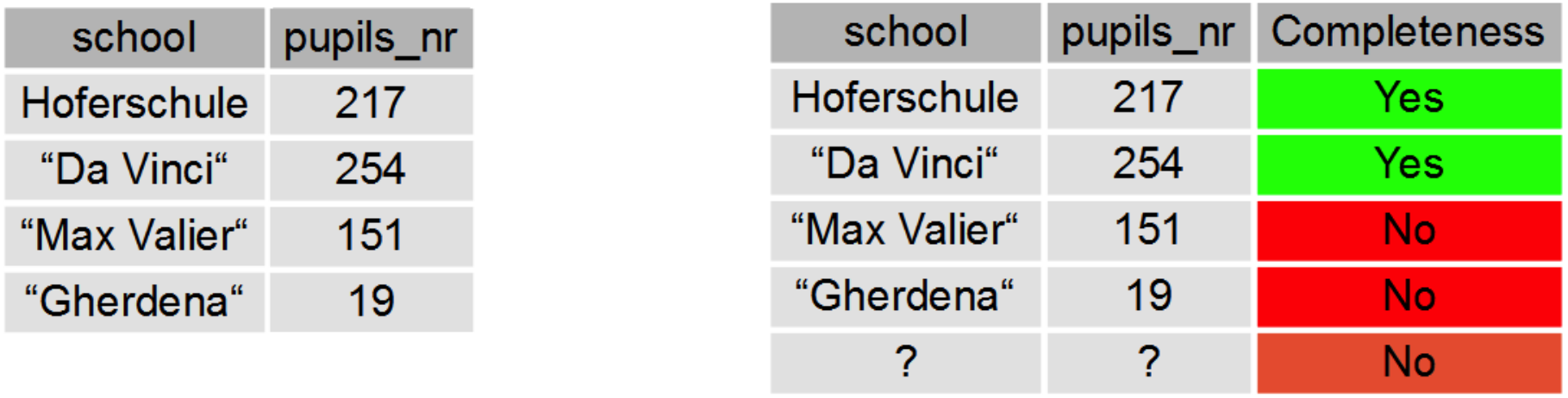
Formally, for a query $Q$ a dimension is a set of distinguished variables of $Q$ . Originally, dimension analysis was meant especially for the arguments of a GROUP BY expression in a query, however it can also be used with other distinguished variables of a query. Assume a query $Q(\bar{x}){:\!-}\,B(\bar{x},\bar{y})$ cannot be guaranteed to be complete in a specific state of a process. For a dimension $\bar{v}\subseteq\bar{x}$ , the analysis can be done as follows:

(i)

Calculate the result of $Q^{\prime}(\bar{v}){:\!-}\,B(\bar{x},\bar{y})$ over $D^{a}$ .
(ii)

For each tuple $\bar{c}$ in $Q^{\prime}(D^{a})$ , check whether $s,D^{a}\models\mathit{Compl}(Q[\bar{v}/\bar{c}])$ . This tells whether the query is complete for the values $\bar{c}$ of the dimension $V$ .
(iii)

To check whether further values are possible, one has to guess a new value $\bar{c}_{new}$ for the dimension and show that $Q[\bar{v}/\bar{c}_{new}]$ is not complete in the current state. For the guess one has to consider only the constants in the database plus a fixed set of new constants, hence the number of possible guesses is polynomial for a fixed dimension $\bar{v}$ .

Step 2 corresponds to deciding for each tuple with a certain value in $Q(D^{a})$ , whether it is complete or not (color red or green in Figure 7.6, right table), Step 3 to deciding whether there can be additional values (bottom row in Figure 7.6, right table).

48.4 Complexity of Completeness Verification

In the previous sections we have seen that completeness verification can be solved using query containment. Results on query containment are already reported in Section 14.3. The results presented here follow from Theorems 7.10 and 7.15, and are summarized in Figure 7.7. We distinguish between the problem of runtime verification, which has the same complexity as query containment, and design-time verification, which, in principle requires to solve query containment exponentially often. Notable however is that in most cases the complexity of runtime verification is not higher than the one of design-time verification.

The results on linear relational and linear conjunctive queries, i.e., conjunctive queries without selfjoins and without or with comparisons, are borrowed from [72]. The result on relational queries is reported in [77], and that on conjunctive queries from [84]. As for integrity constraints, the result for databases satisfying finite domain constraints is reported in [72] and for databases satisfying keys and foreign keys in [14].

Query/QATS language $\mathcal{L}$	Runtime-verification: Complexity of $\mathsf{\mathit{UCont}}(\mathcal{L},\mathcal{L})$ and $\mathit{EntC}(\mathcal{L})$ “ $(\pi\models\mathit{Compl}(Q))$ ”?	Design-time verification: Complexity of “ $s\models\mathit{Compl}(Q)$ ”?
Linear relational queries	PTIME	in $\mathrm{coNP}$
Linear conjunctive queries	$\mathrm{coNP}$ -complete	$\mathrm{coNP}$ -complete
Relational queries	NP-complete	in $\Pi_{2}^{P}$
Relational queries over databases with finite domains	$\Pi_{2}^{P}$ -complete	$\Pi_{2}^{P}$ -complete
Conjunctive queries	$\Pi_{2}^{P}$ -complete	$\Pi_{2}^{P}$ -complete
Relational queries over databases with keys and foreign keys	in PSPACE	in PSPACE

Figure 7.7: Complexity of design-time and runtime verification for different query languages.

49 Extracting Transition Systems from Petri Nets

Transition systems are a very basic formalism for describing the semantics of business processes. For business processes itself, the quasi-standard for process models is the business process modeling notation (BPMN). Large parts of BPMN are well founded in coloured Petri nets. In turn, the models of coloured Petri nets are represented by its reachability graph, which is a transition system. It is therefore not surprising that the annotations of transition systems with real-world and copy effects can also be expressed on the level of coloured Petri nets.

Informally, coloured Petri nets (CPN) are systems in which tokens of different types can move and interact according to defined actions [49]. An example of a CPN that is annotated with real-world and copy effects is shown in Figure 7.8. In this CPN, there exist three types of tokens: Time, persons and schools, which initially populate the places on the left side in top-down order. The actions can be executed whenever there are tokens in all the input places, e.g., the action “Enroll yourself” can be executed whenever there there is a time token in the first place, a person token in the second place and a school token in the third place.

When annotating Petri nets with real-world and copy effects, we can now use the variables of the actions also in the effect specifications: For instance, the real-world effect of the action “Decide enrollments of a school” allows to create records enrolled(n,s) for pupils who expressed an enrollment desire at the school which performs this action.

Notice that while already coloured Petri nets also allow some representation of data via the tokens, CPN annotated with real-world and copy effects go clearly beyond this, because (1) copy actions are a kind of universally quantified transitions, (2) they allow the introduction of new values, and (3) allow the verification for arbitrary starting databases.

The semantics of Coloured Petri nets are their reachability graphs, which, in turn, are transition systems. A common class of well-behaved Petri nets are bound Petri nets. A Petri net is bound by a value $k$ , if the number of tokens in all reachable states is less or equal to $k$ . For $k$ -bound Petri nets, their reachability graph is at most exponential in $k$ . Thus, completeness verification over coloured Petri nets can be reduced to completeness verification over exponential transition systems.

Figure 7.8: Enrollment both from the perspective of schools and students modelled in a CPN. A desirable property to check is that when the action “Publish statistics” is executed, the data about enrolments is complete, which in this example is the case.

50 Related Work

In the BPM context, there have been attempts to model data quality issues, like in [13, 76, 7]. However, these approaches mainly discussed general methodologies for modeling data quality requirements in BPMN, but did not provide methods to asses their fulfillment. In this chapter, we claim that process formalizations are an essential source for learning about data completeness and show how data completeness can be verified. In particular, our contributions are (1) to introduce the idea of extracting information about data completeness from processes manipulating the data, (2) to formalize processes that can both interact with the real-world and record information about the real-world in an information system, and (3) to show how completeness can be verified over such processes, both at design and at execution time.

Our approach leverages on two assumptions related to how the data manipulation and the process control-flow are captured. From the data point of view, we leverage on annotations that suitably mediate between expressiveness and tractability. More specifically, we rely on annotations modeling that new information of a given type is acquired in the real world, or that some information present in the real world is stored into the information system. We do not explicitly consider the evolution of specific values for the data, as incorporating full-fledged data without any restriction would immediately make our problem undecidable, being simple reachability queries undecidable in such a rich setting [22, 8, 9]. From the control-flow point of view, we are completely orthogonal to process specification languages. In particular, we design our data completeness algorithms over (labeled) transition systems, a well-established mathematical structure to represent the execution traces that can by produced according to the control-flow dependencies of the (business) process model of interest. Consequently, our approach can in principle be applied to any process modeling language, with the proviso of annotating the involved activities. We are in particular interested in providing automated reasoning facilities to answer whether a given query can be answered with complete information given a target state or a sequence of activities.

51 Summary

In this chapter we have discussed that data completeness analysis should take into account the processes that manipulate the data. In particular, we have shown how process models can be annotated with effects that create data in the real world and effects that copy data from the real world into an information system. We have then shown how one can verify the completeness of queries over transition systems that represent the execution semantics of such processes. It was shown that, similarly to the previous chapters, the problems here are closely related to the problem of query containment, although now, it may be the case that exponentially many containments have to be solved for one completeness check. We also showed that completeness checking is easier when the trace of the process is known.

We focused on the process execution semantics in terms of transition systems. The results would allow the realization of a demonstration system to annotate high-level business process specification languages (such as BPMN or YAWL), extract the underlying quality-aware transition systems, and apply the techniques here presented to check completeness.

^†^†margin: 8 Discussion

In the previous chapters we have discussed how to analyze the completeness of query answers over databases using metadata about the completeness of parts of the data. A critical prerequisite for doing such analysis is to actually obtain such completeness metadata, and to have reasons to believe that this metadata is correct. Also, the practical implications of the presented complexity results and the technical integration of completeness reasoning into existing software landscapes are important issues. In the following, we discuss these issues.

Obtaining Completeness Statements and Ensuring Statement Correctness

In the setting of company databases, especially fast-changing transactional databases that possibly get integrated into data warehouses regularly, in order to have up-to-date completeness metadata, completeness statement generation needs to be automated as much as possible. Where data creation is done automatically (e.g., sensor data), it could be feasible to also generate completeness statements automatically. Where data is submitted manually (for instance, a human presses a "submit" button), completeness statement generation should be bound to the data submission. That is, whenever data is submitted, the user is asked (or forced) to also make statements about the (in-)completeness of the submitted data. This is crucial, because commonly the stakeholder that will know most about the completeness of the data is the one who submits the data.

In settings where the knowledge about completeness is not captured directly at data creation, later attempts to get completeness statements will require manual inspection and may be tricky, as often information about data provenance is not maintained well. This may e.g. be a problem when a database with completeness metadata is merged with another database without such completeness information, e.g. after an acquisition.

In the settings of crowd-based data such as OpenStreetMap or of integrated data without any quality guarantees such as on the Semantic Web, there is no way to enforce the generation of completeness metadata. Instead, completeness metadata will need to be generated and maintained based on mutual ratings and trust levels.

Practical Complexity

While some theoretical complexity results presented in this thesis may seem as if implementations could be very challenging, most discussed schema-level reasoning problems are reduced to query containment, which, for the languages discussed, is solved in existing DBMS every day. We thus expect little runtime challenges when implementing schema level reasoning using existing techniques for containment.

On the other hand, the results for reasoning wrt. a database instance for which we showed a PTIME data complexity still pose a big challenge: Even a linear data complexity may be not feasible for large data warehouses, thus, for these results, more research is needed before they can be implemented.

Set/bag disambiguation for TC-QC Reasoning

A major complication in the presented results is the disambiguation between set and bag semantics for queries. As Proposition 3.18 however shows, TC-QCentailment reasoning for queries under bag and set semantics only differs in cases where the queries under set semantics not minimal, and can be synchronized again using query minimization. As for all instances of $\mbox{{TC-QC}}^{s}(\mathcal{L}_{1},\mathcal{L}_{2})$ with $\mathcal{L}_{1}=\mathcal{L}_{2}$ , the complexity is the same as that of minimization of queries in $\mathcal{L}_{1}$ , the separate discussion of the reasoning for queries under set semantics in Section 14.3 may give the wrong impression that the problems are very different, while in fact in all but one case they can be dealt with by the same algorithm.

Technical Integration

The technical integration of completeness reasoning into data management software remains an open problem. We can only conjecture that a completeness reasoner component will require deep integration into the existing data management software landscape.

First, the components that create completeness statements would need to be integrated into software for creating and manipulation database content, e.g. MS Access, SAP software, or custom-made web interfaces.

Second, the component that perform the actual reasoning should be integrated with the DBMS, e.g. as a plugin, in order to allow the execution of reasoning at the same time as query execution.

Third, the components for visualizing completeness information need to be embedded into the software that is used to show query results, such as management cockpits, web portals or business intelligence tools such as Qlikview.

Impact

Parts of the theory presented in this thesis have been implemented by Savkovic et al. in a demonstration system called MAGIK [78, 79]. The reasoning is MAGIK is performed by translating the reasoning problems into logical programs, which are then solved by the DLV reasoner ¹³¹³ 13 http://www.dlvsystem.com/html/DLV_User_Manual.html. MAGIK can also reasoning tasks that are not discussed in this thesis, namely reasoning wrt. foreign keys and computing the most general complete specializations or the least general complete generalization of a query that are not complete.

References

[1] Serge Abiteboul, Richard Hull, and Victor Vianu. Foundations of databases. In Addison-Wesley, 1995.
[2] Serge Abiteboul, Paris Kanellakis, and Gösta Grahne. On the representation and querying of sets of possible worlds. Theoretical Computer Science, 78(1):159–187, 1991.
[3] Serge Abiteboul, Luc Segoufin, and Victor Vianu. Representing and querying XML with incomplete information. ACM TODS, 31(1):208–254, 2006.
[4] Foto N. Afrati. Rewriting conjunctive queries determined by views. In MFCS, pages 78–89, 2007.
[5] Keith Alexander, Richard Cyganiak, Michael Hausenblas, and Jun Zhao. Describing linked datasets with the VoID vocabulary. Technical report, W3C, 2011.
[6] Marcelo Arenas, Claudio Gutierrez, and Jorge Pérez. On the semantics of SPARQL. In Semantic Web Information Management, pages 281–307. Springer-Verlag Berlin Heidelberg, 2010.
[7] Sugato Bagchi, Xue Bai, and Jayant Kalagnanam. Data quality management using business process modeling. In Services Computing, 2006. SCC’06. IEEE International Conference on, 2006.
[8] Babak Bagheri Hariri, Diego Calvanese, Giuseppe De Giacomo, Riccardo De Masellis, and Paolo Felli. Foundations of relational artifacts verification. In Proc. of the 9th Int. Conference on Business Process Management (BPM 2011), volume 6896 of Lecture Notes in Computer Science, pages 379–395. Springer, 2011.
[9] Babak Bagheri Hariri, Diego Calvanese, Giuseppe De Giacomo, Alin Deutsch, and Marco Montali. Verification of relational data-centric dynamic systems with external services. In Proc. of the 32nd ACM SIGACT SIGMOD SIGART Symp. on Principles of Database Systems (PODS 2013), 2013.
[10] Christel Baier and Joost-Pieter Katoen. Principles of Model Checking. The MIT Press, 2008.
[11] Jit Biswas, Felix Naumann, and Qiang Qiu. Assessing the completeness of sensor data. In Proc. DASFAA, pages 717–732, 2006.
[12] Dan Brickley and R.V. Guha. RDF vocabulary description language 1.0: RDF schema. Technical report, W3C, 2004.
[13] Hugo Bringel, Artur Caetano, and José M. Tribolet. Business process modeling towards data quality: A organizational engineering approach. In ICEIS (3), 2004.
[14] Andrea Calı, Domenico Lembo, and Riccardo Rosati. Query rewriting and answering under constraints in data integration systems. In Proc. of the 18th Int. Joint Conf. on Artificial Intelligence (IJCAI 2003), pages 16–21, 2003.
[15] Irene Celino, Dario Cerizza, Simone Contessa, Marta Corubolo, Daniele Dell’Aglio, Emanuele d. Valle, and Stefano Fumeo. Urbanopoly - a social and location-based game with a purpose to crowdsource your urban data. In SocialCom/PASSAT, pages 910–913, 2012.
[16] Ashok K. Chandra and Philip M. Merlin. Optimal implementation of conjunctive queries in relational data bases. In STOC, pages 77–90, 1977.
[17] Keith L Clark. Negation as failure. In Logic and data bases, pages 293–322. Springer, 1978.
[18] Edgar F. Codd. A relational model of data for large shared data banks. Commun. ACM, 13(6):377–387, June 1970.
[19] Edgar F. Codd. Understanding relations (installment #7). FDT – Bulletin of ACM SIGMOD, 7(3):23–28, 1975.
[20] Edgar F. Codd. Missing information (applicable and inapplicable) in relational databases. SIGMOD Record, 15(4):53–78, 1986.
[21] Sarah Cohen, Werner Nutt, and Yehoshua Sagiv. Deciding equivalences among conjunctive aggregate queries. J. ACM, 54(2), 2007.
[22] Elio Damaggio, Alin Deutsch, Richard Hull, and Victor Vianu. Automatic verification of data-centric business processes. In Proc. of the 9th Int. Conference on Business Process Management (BPM 2011), Lecture Notes in Computer Science, pages 3–16. Springer, 2011.
[23] Fariz Darari. Completeness reasoning for linked data queries. Master Thesis, Free University of Bozen-Bolzano, Italy and Technische Universitaet Dresden, Germany, 2013.
[24] Fariz Darari, Werner Nutt, Giuseppe Pirrò, and Simon Razniewski. Completeness statements about RDF data sources and their use for query answering. In International Semantic Web Conference (1), pages 66–83, 2013.
[25] Robert Demolombe. Answering queries about validity and completeness of data: From modal logic to relational algebra. In FQAS, pages 265–276, 1996.
[26] Robert Demolombe. Database validity and completeness: Another approach and its formalisation in modal logic. In KRDB, pages 11–13, 1999.
[27] Marc Denecker, Alvaro Cortés-Calabuig, Maurice Bruynooghe, and Ofer Arieli. Towards a logical reconstruction of a theory for locally closed databases. ACM TODS, 35(3), 2010.
[28] Patrick Doherty, Witold Lukaszewicz, and Andrzej Szalas. Efficient reasoning using the local closed-world assumption. In AIMSA, pages 49–58, 2000.
[29] Charles Elkan. Independence of logic database queries and updates. In Proc. PODS, pages 154–160, 1990.
[30] Oren Etzioni, Keith Golden, and Daniel S. Weld. Sound and efficient closed-world reasoning for planning. AI, 89(1-2):113–148, 1997.
[31] Ron Fagin, Phokion Kolaitis, Renée Miller, and Lucian Popa. Data exchange: Semantics and query answering. In Proc. ICDT, pages 207–224, 2002.
[32] Wenfei Fan and Floris Geerts. Relative information completeness. In PODS, pages 97–106, 2009.
[33] Wenfei Fan and Floris Geerts. Capturing missing tuples and missing values. In PODS, pages 169–178, 2010.
[34] Wenfei Fan, Floris Geerts, and Lixiao Zheng. View determinacy for preserving selected information in data transformations. Inf. Syst., 37(1):1–12, 2012.
[35] Charles Farré, Werner Nutt, Erneste Teniente, and Toni Urpí. Containment of conjunctive queries over databases with null values. In ICDT, pages 389–403, 2007.
[36] Ivan P. Fellegi and Alan B. Sunter. A theory for record linkage. Journal of the American Statistical Association, 64(328):1183–1210, 1969.
[37] Enrico Franconi and Sergio Tessaris. On the logic of SQL nulls. In Alberto Mendelzon Workshop on Foundations of Data Management, pages 114–128, 2012.
[38] Christian Fürber and Martin Hepp. Using SPARQL and SPIN for data quality management on the Semantic Web. In BIS, pages 35–46, 2010.
[39] A Blanton Godfrey. Juran’s quality handbook. McGraw Hill, 1999.
[40] Ralf Hartmut Güting. An introduction to spatial database systems. VLDB J., 3(4):357–399, 1994.
[41] Mordechai Haklay. How good is volunteered geographical information? A comparative study of OpenStreetMap and Ordnance Survey datasets. Environment and Planning. B, Planning & Design, 37(4):682, 2010.
[42] Mordechai Haklay and Claire Ellul. Completeness in volunteered geographical information—the evolution of OpenStreetMap coverage in England (2008-2009). Journal of Spatial Information Science, 2010.
[43] Steve Harris and Andy Seaborne. SPARQL 1.1 query language. Technical report, W3C, 2013.
[44] Andreas Harth and Sebastian Speiser. On completeness classes for query evaluation on linked data. In AAAI, 2012.
[45] Olaf Hartig, Christian Bizer, and Johann-Christoph Freytag. Executing SPARQL queries over the web of linked data. In International Semantic Web Conference, pages 293–309, 2009.
[46] T. Heath and C. Bizer. Linked Data: Evolving the Web into a Global Data Space. Synthesis Lectures on the Semantic Web. Morgan & Claypool Publishers, 2011.
[47] Tomasz Imieliński and Witold Lipski, Jr. Incomplete information in relational databases. J. ACM, 31:761–791, 1984.
[48] T. S. Jayram, Phokion G. Kolaitis, and Erik Vee. The containment problem for real conjunctive queries with inequalities. In PODS, pages 80–89, 2006.
[49] Kurt Jensen. Coloured petri nets. Petri nets: central models and their properties, pages 248–299, 1987.
[50] Anthony C. Klug. On conjunctive queries containing inequalities. J. ACM, 35(1):146–160, 1988.
[51] Graham Klyne and Jeremy J. Carroll. Resource Description Framework (RDF): Concepts and abstract syntax. Technical report, W3C, 2004.
[52] Edith Law and Luis von Ahn. Human Computation. Synthesis Lectures on Artificial Intelligence and Machine Learning. Morgan & Claypool Publishers, 2011.
[53] Yang W. Lee, Leo Pipino, James D. Funk, and Richard Y. Wang. Journey to data quality. In MIT Press, 2006.
[54] Maurizio Lenzerini. Data integration: A theoretical perspective. In Proceedings of the Twenty-first ACM SIGMOD-SIGACT-SIGART Symposium on Principles of Database Systems, PODS ’02, pages 233–246, New York, NY, USA, 2002. ACM.
[55] Andrés Letelier, Jorge Pérez, Reinhard Pichler, and Sebastian Skritek. Static analysis and optimization of semantic web queries. In PODS, pages 89–100, 2012.
[56] Alon Y. Levy. Obtaining complete answers from incomplete databases. In Proceedings of the International Conference on Very Large Data Bases, pages 402–412, 1996.
[57] Alon Y. Levy, Alberto O. Mendelzon, Yehoshua Sagiv, and Divesh Srivastava. Answering queries using views. In PODS, pages 95–104, 1995.
[58] Peter Mooney, Padraig Corcoran, and Adam C. Winstanley. Towards quality metrics for OpenStreetMap. In Proceedings of the 18th SIGSPATIAL International Conference on Advances in Geographic Information Systems, pages 514–517. ACM, 2010.
[59] Amihai Motro. Integrity = Validity + Completeness. ACM TODS, 14(4):480–502, 1989.
[60] Sergio Muñoz, Jorge Pérez, and Claudio Gutierrez. Simple and efficient minimal RDFS. J. Web Sem., 7(3):220–234, 2009.
[61] Felix Naumann, Johann-Christoph Freytag, and Ulf Leser. Completeness of integrated information sources. Inf. Syst., 29:583–615, September 2004.
[62] Charalampos Nikolaou and Manolis Koubarakis. Incomplete information in rdf. CoRR, abs/1209.3756, 2012.
[63] Werner Nutt, Sergey Paramonov, and Ognjen Savkovic. An ASP approach to query completeness reasoning. TPLP, 13(4-5-Online-Supplement), 2013.
[64] Werner Nutt and Simon Razniewski. Completeness of queries over SQL databases. In CIKM, pages 902–911, 2012.
[65] Daniel Pasaila. Conjunctive queries determinacy and rewriting. In ICDT, pages 220–231, 2011.
[66] Peter F. Patel-Schneider and Enrico Franconi. Ontology constraints in incomplete and complete data. In International Semantic Web Conference (1), pages 444–459, 2012.
[67] Jorge Pérez, Marcelo Arenas, and Claudio Gutierrez. Semantics and complexity of SPARQL. ACM TODS, 34(3):16, 2009.
[68] Francois Picalausa and Stijn Vansummeren. What are real SPARQL queries like? In SWIM, 2011.
[69] Simon Razniewski. Completeness of queries over incomplete databases. Diplomarbeit, Technische Universitaet Dresden, Germany, 2010.
[70] Simon Razniewski, Marco Montali, and Werner Nutt. Verification of query completeness over processes. In BPM, pages 155–170, 2013.
[71] Simon Razniewski, Marco Montali, and Werner Nutt. Verification of query completeness over processes [extended version]. CoRR, abs/1306.1689, 2013.
[72] Simon Razniewski and Werner Nutt. Completeness of queries over incomplete databases. In VLDB, 2011.
[73] Simon Razniewski and Werner Nutt. Assessing the completeness of geographical data (short paper). In BNCOD, 2013.
[74] Raymond Reiter. On closed world data bases. Springer, 1978.
[75] Raymond Reiter. A sound and sometimes complete query evaluation algorithm for relational databases with null values. J. ACM, 33(2):349–370, 1986.
[76] Alfonso Rodríguez, Angelica Caro, Cinzia Cappiello, and Ismael Caballero. A BPMN extension for including data quality requirements in business process modeling. In BPMN, 2012.
[77] Yehoshua Sagiv and Mihalis Yannakakis. Equivalence among relational expressions with the union and difference operation. In VLDB, pages 535–548, 1978.
[78] Ognjen Savkovic, Paramita Mirza, Sergey Paramonov, and Werner Nutt. Magik: managing completeness of data. In CIKM, pages 2725–2727, 2012.
[79] Ognjen Savkovic, Paramita Mirza, Alex Tomasi, and Werner Nutt. Complete approximations of incomplete queries. PVLDB, 6(12):1378–1381, 2013.
[80] Andy Seaborne, Axel Polleres, Lee Feigenbaum, and Gregory T. Williams. SPARQL 1.1 federated query. Technical report, W3C, 2013.
[81] Luc Segoufin and Victor Vianu. Views and queries: Determinacy and rewriting. In Proc. PODS, pages 49–60, 2005.
[82] Wenzhong Shi, Peter Fisher, and Michael F. Goodchild. Spatial Data Quality. CRC, 2002.
[83] Giorgios Stoilos, Bernardo C. Grau, and Ian Horrocks. How incomplete is your semantic web reasoner? In AAAI, 2010.
[84] Ron van der Meyden. The complexity of querying indefinite data about linearly ordered domains. In PODS, pages 331–345, 1992.
[85] Ron van der Meyden. Logical approaches to incomplete information: A survey. In Logics for Databases and Information Systems, pages 307–356, 1998.
[86] Richard Y Wang and Diane M Strong. Beyond accuracy: What data quality means to data consumers. Journal of management information systems, pages 5–33, 1996.
[87] T. Wang and J. Wang. Visualisation of spatial data quality for internet and mobile GIS applications. Journal of Spatial Science, 49(1):97–107, 2004.
[88] William E Winkler. Overview of record linkage and current research directions. In Bureau of the Census. Citeseer, 2006.
[89] Howard J. Hamilton Xin Wang and Yashu Bither. An ontology-based approach to data cleaning. Department of Computer Science, University of Regina, 2005.

^†^†margin: 9 Notation Table

The listing below contains common notation used throughout this thesis. Notation that is specific to a single chapter is not listed here.

Symbol	Meaning
$\Sigma$	relational database schema
$A$	relational atom
$\mathit{dom}$	domain, infinite set of constants
$D$	database, set of ground atoms
$c$	constant
$\bar{d}$	tuple of constants
$x,y,z,w$	variables
$t$	term, constant or variable
$R,(S,T)$	relation names
$Q$	conjunctive query
$B$	body of a conjunctive query
$\bar{x}$	distinguished variables of a query
$\bar{y}$	nondistinguished variables of a query
$L$	relational part of a body
$M$	comparisons
$G$	condition, set of atoms
$\cdot^{s}$	set semantics
$\cdot^{b}$	bag semantics
$D^{i}$	ideal database
$D^{a}$	available database
$\mathcal{D}$	incomplete database, pair of an ideal and an available database
$C$	table completeness statement
$Q_{C}$	query associated to a table completeness statement
$v$	valuation, mapping from variables into constants; sometimes also Greek letters $(\sigma,\theta,\delta)$
$T_{C}$	transformator function for a TC statement, maps databases into databases
$\mathit{Compl}(Q)$	query completeness statement for a query $Q$
$\mathcal{L}$	query language
$\mathit{Cont}$	containment problem of a query in a query
$\mathsf{\mathit{UCont}}$	containment problem of a query in a union of queries
TC-TC	entailment problem of table completeness by table completeness
TC-QC	entailment problem of table completeness by query completeness
TC-QC	entailment problem of query completeness by query completeness

Acknowledgement

Publication Overview

Conference Publications

Other Publications

††margin: 1 Introduction

1 Data Quality and Data Completeness

2 Motivation

3 Contribution

4 Structure

††margin: 2 Preliminaries

5 Running Example

6 Relational Databases

Definition 2.1.

Example 2.2.

7 Database Queries

Example 2.3.

Definition 2.4 (Conjunctive Query).

Remark 2.5 (Notation).

Classes of Conjunctive Queries

Example 2.6.

Remark 2.7 (Freezing).

8 Incomplete Databases

Definition 2.8.

Example 2.9.

9 Query Completeness

Definition 2.10 (Query Completeness).

Definition 2.11.

Example 2.12.

Remark 2.13 (Terminology).

10 Table Completeness

Definition 2.14 (Table Completeness).

Definition 2.15.

Example 2.16.

Remark 2.17 (Notation).

Example 2.18.

Example 2.19.

11 Complexity of Query Containment

Definition 2.20.

11.1 𝑈𝐶𝑜𝑛𝑡⁡(ℒLRQ,ℒLCQ)\mathit{UCont}(\mathcal{L}_{{\rm{LRQ}}},\mathcal{L}_{{\rm{LCQ}}}) is coNP\mathrm{coNP}-hard

Lemma 2.21.

Proof.

Corollary 2.22.

11.2 𝐶𝑜𝑛𝑡⁡(ℒRQ,ℒLRQ)\mathit{Cont}(\mathcal{L}_{{\rm{RQ}}},\mathcal{L}_{{\rm{LRQ}}}) is NP\mathrm{NP}-hard

Lemma 2.23.

Proof.

Corollary 2.24.

11.3 𝐶𝑜𝑛𝑡⁡(ℒRQ,ℒLCQ)\mathit{Cont}(\mathcal{L}_{{\rm{RQ}}},\mathcal{L}_{{\rm{LCQ}}}) is Π2P\Pi_{2}^{P}-hard

Lemma 2.25.

Proof.

Corollary 2.26.

12 Entailment

Example 2.27.

††margin: 3 Completeness Reasoning

13 Table Completeness Entailing Table Completeness

Example 3.1.

Theorem 3.2.

Proof.

14 Table Completeness Entailing Query Completeness

14.1 TC-QC Entailment for Queries under Bag Semantics

Example 3.3.

Theorem 3.4.

Proof.

Theorem 3.5.

Proof.

14.2 Characterizations of Query Completeness under Set Semantics

Example 3.6.

Corollary 3.7.

Proof.

Proposition 3.8.

Proof.

Theorem 3.9.

Proof.

14.3 TC-QC Entailment for Queries under Set Semantics

Theorem 3.10.

Definition 3.11.

Lemma 3.12.

Proof.

Proof of Theorem 3.10.

Lemma 3.13.

Proof.

^†^†margin: 1 Introduction

^†^†margin: 2 Preliminaries

11.1 $\mathit{UCont}(\mathcal{L}_{{\rm{LRQ}}},\mathcal{L}_{{\rm{LCQ}}})$ is $\mathrm{coNP}$ -hard

11.2 $\mathit{Cont}(\mathcal{L}_{{\rm{RQ}}},\mathcal{L}_{{\rm{LRQ}}})$ is $\mathrm{NP}$ -hard

11.3 $\mathit{Cont}(\mathcal{L}_{{\rm{RQ}}},\mathcal{L}_{{\rm{LCQ}}})$ is $\Pi_{2}^{P}$ -hard

^†^†margin: 3 Completeness Reasoning

Theorem 3.27 (Decidability of $\mbox{{QC-QC}}^{b}$ ).

^†^†margin: 4 Databases with Null Values